PBH assisted search for QCD axion dark matter

Abstract

The entropy production prior to BBN era is one of ways to prevent QCD axion with the decay constant $\displaystyle F_{a}\in[10^{12}{\rm GeV},10^{16}{\rm GeV}]$ from overclosing the universe when the misalignment angle is $\displaystyle\theta_{\rm i}=\mathcal{O}(1)$. As such, it is necessarily accompanied by an early matter-dominated era (EMD) provided the entropy production is achieved via the decay of a heavy particle. In this work, we consider the possibility of formation of primordial black holes during the EMD era with the assumption of the enhanced primordial scalar perturbation on small scales ($\displaystyle k>10^{4}{\rm Mpc}^{-1}$). In such a scenario, it is expected that PBHs with axion halo accretion develop to ultracompact minihalos (UCMHs). We study how UCMHs so obtained could be of great use in the experimental search for QCD axion dark matter with $\displaystyle F_{a}\in[10^{12}{\rm GeV},10^{16}{\rm GeV}]$.

I Introduction

The charm of QCD axion lies in the fact that it could not only explain the null observation of CP violation in the strong sector in the Standard Model (SM), but also serve as a good dark matter (DM) candidate. As a pseudo Nambu-Goldstone boson resulting from the spontaneous breaking of the global $\displaystyle U(1)$ anomalous with respect to $\displaystyle SU(3)_{c}$ in the SM, its potential is generated by the instanton-induced fermionic determinantal interaction when QCD becomes non-perturbative. Thereby the axion mass ($\displaystyle m_{a}$) and its decay constant ($\displaystyle F_{a}$) is subject to the relation $\displaystyle m_{a}F_{a}\sim m_{\pi}F_{\pi}\simeq(100{\rm MeV})^{2}$ with $\displaystyle m_{\pi}$ and $\displaystyle F_{\pi}$ the pion mass and decay constant.

Concerning the decay constant, the lower bound based on the stellar cooling process reads $\displaystyle\sim 10^{9}{\rm GeV}$ Raffelt (2008). For a QCD axion model where the axion is the DM candidate and the initial misalignment angle is $\displaystyle\theta_{\rm i}\equiv a_{i}/F_{a}=\mathcal{O}(1)$, how high $\displaystyle F_{a}$ could be is determined by the relic abundance of the axion today ($\displaystyle\Omega_{a}h^{2}$). And $\displaystyle\Omega_{a}h^{2}=\Omega_{\rm DM}h^{2}$ holds for $\displaystyle F_{a}\simeq 10^{12}{\rm GeV}$ when the standard cosmological history without the early matter-dominated (EMD) era is assumed. QCD axion window so obtained $\displaystyle 10^{9}{\rm GeV}\lesssim F_{a}\lesssim 10^{12}{\rm GeV}$ indicates the mass range $\displaystyle\mathcal{O}(10^{-6}){\rm eV}\leq m_{a}\leq\mathcal{O}(10^{-3}){\rm eV}$ for the QCD axion.

The upper bound of $\displaystyle F_{a}$ above, however, can be relaxed provided there is a mechanism either to deplete the relic abundance of axion or to induce $\displaystyle\theta_{\rm i}<\!\!<\mathcal{O}(1)$ before oscillation starts. For the former, as an example, when the axion is coupled to the hidden photon, a rapid axion energy conversion thanks to tachyonic instability in dark photon production could allow for the higher $\displaystyle F_{a}$ than $\displaystyle 10^{12}{\rm GeV}$ Agrawal et al. (2018); Kitajima et al. (2018). For the later, one may consider the possibility of an enhanced axion mass during inflation which results in a suppressed $\displaystyle\theta_{\rm i}$ after inflation Dvali (1995); Co et al. (2019); Buen-Abad and Fan (2019).

The assumption of the entropy production caused by the late time decay of a heavy particle is another way of the energy depletion. This is particularly convincing possibility when an axion model is considered with supersymmetry (SUSY) or in light of string theory de Carlos et al. (1993); Banks et al. (1994); Conlon (2006); Svrcek and Witten (2006); Choi and Jeong (2007); Acharya et al. (2014). A heavy saxion and moduli fields are generic prediction thereof and hence the axion cosmology becomes naturally incorporated with sources of the entropy production. Insofar as the decay takes place before $\displaystyle T\simeq 5{\rm MeV}$ (the temperature of the thermal bath) is reached, the extra radiation arising from the decay of the heavy particle could dilute the energy density of the universe contributed by axion without spoiling the relic abundance of primordial light elements Steinhardt and Turner (1983); Kawasaki et al. (1996, 2016a).

The presence of such a heavy degree of freedom ($\displaystyle\sigma$) often implies the non-standard cosmology featured by an EMD era prior to BBN. Soon after starting oscillation, $\displaystyle\sigma$ behaves as a matter ($\displaystyle\rho_{\sigma}\propto R^{-3}$) so as to start to dominate the energy budget of the universe. Therefore, a hunting strategy for the axion with a large decay constant $\displaystyle F_{a}\in[10^{12}{\rm GeV},10^{16}{\rm GeV}]$ could concern phenomenologies attributable to EMD era. One of these could be the fact that the growth rate of the perturbation is linear, differing from that in radiation dominated era (logarithmic). If primordial fluctuations re-entering the horizon during the EMD era are large enough, relatively more efficient formation of the primordial black holes (PBH) than that in the standard cosmology can be expected.

The constraint on the power spectrum of the primordial curvature perturbation on small scales $\displaystyle k\gtrsim\mathcal{O}(10){\rm Mpc}^{-1}$ is still not as strong as the CMB constraint on larges scales $\displaystyle k\lesssim 0.2{\rm Mpc}^{-1}$. Thus, having much larger primordial power spectrum on small scales $\displaystyle k\gtrsim\mathcal{O}(10){\rm Mpc}^{-1}$ than in the CMB scale still remains viable, which could possibly develop to formation of heavy enough PBHs with $\displaystyle M_{\rm PBH}\gtrsim\mathcal{O}(10^{-16})M_{\odot}$ that does not evaporate to date. If so, accretion of the axion halo around PBHs is expected, which produces the so-called ultracompact minihalo (UCMH) heavier than $\displaystyle M_{\rm PBH}$.

In this paper, motivated by the interest in UV physics-supported axion with the large decay constant $\displaystyle F_{a}=\mathcal{O}(10^{16}){\rm GeV}$ and the EMD era prior to BBN era, we study axion cosmology with UCMH made up of PBH and axion halo. We consider the QCD axion decay constant range $\displaystyle F_{a}\in[10^{12}{\rm GeV},10^{16}{\rm GeV}]$. We shall assume two reheating periods: the reheating due to the inflaton right after the inflation (rh1) and the reheating due to the heavy scalar particle $\displaystyle\sigma$ (saxion or moduli) decay prior to BBN era (rh2). Due to our interest in the specific experimental ways of probing the scenario, we will discuss two cases in this work: Case I with $\displaystyle M_{\rm PBH}\lesssim\mathcal{O}(10^{-6})M_{\odot}$ and Case II with $\displaystyle M_{\rm PBH}=\mathcal{O}(1)M_{\odot}$.

In Sec. II, we review the axion relic abundance in the standard cosmology and shows how it could be modified in the presence of entropy production. In Sec. III, we go through the details of the numerical computation for the relic abundance of axion DM in the presence of EMD era and the entropy release from the heavy particle decay. In Sec. IV, with specification of our assumption for the power spectrum of primordial curvature perturbation, we compute the mass and the fraction of PBH in DM as functions of the heavy particle mass and reheating temperature (rh2). And then in Sec. V, we explain how the PBH could develop to UCMH. In Sec. VI, we discuss how the large decay constant axion picture can be experimentally probed based on the enhanced axion dark matter local density due to the tidal stream arising from disruption of UCMH characterized by $\displaystyle M_{\rm PBH}\lesssim\mathcal{O}(10^{-6})M_{\odot}$ (case I). In Sec. VII, we study another way of indirect detection of axions with $\displaystyle F_{a}\in[10^{12}{\rm GeV},5\times 10^{13}{\rm GeV}]$ through detection of the transient radio signal generated from encounter between a neutron star and UCMH characterized by $\displaystyle M_{\rm PBH}=\mathcal{O}(1)M_{\odot}$. Finally, in Sec. VIII, we conclude by summarizing the main points of the scenario and discussing its future outlook.

II Diluting Axion Relic Abundance by Entropy Production

Having $\displaystyle F_{a}\in[10^{12}{\rm GeV},10^{16}{\rm GeV}]$ for the QCD axion in mind, PQ-breaking is expected to take place before or during the inflation in the scenario we consider, which precludes generation of the associated topological defects and axion production from their decay. This makes the misalignment mechanism the dominant non-thermal axion production channel aside from the negligible thermal production from the thermal plasma via particle scatterings and decays Preskill et al. (1983); Dine and Fischler (1983); Abbott and Sikivie (1983).

In the standard cosmology without an EMD era, when the Hubble expansion rate becomes comparable to the axion mass ($\displaystyle m_{a}$), the axion field starts coherent oscillation. Given that the axion energy density ($\displaystyle\rho_{a}$) scales as $\displaystyle\rho_{a}\propto R^{-3}$ with $\displaystyle R$ the scale factor and the number density ($\displaystyle n_{a}$) is $\displaystyle\rho_{a}=m_{a}n_{a}$, the comoving number density ($\displaystyle Y_{a}\equiv n_{a}/s$) of axion becomes conserved since then because the entropy density $\displaystyle s$ scales as $\displaystyle s\propto R^{-3}$.

Depending on whether the oscillation gets started before and after the QCD phase transition, the axion relic abundance expression could be different due to the different oscillation temperature $\displaystyle T_{\rm osc}\simeq\sqrt{m_{a}(T_{\rm osc})M_{P}}$ Fox et al. (2004). For $\displaystyle F_{a}\lesssim 2\times 10^{15}{\rm GeV}$ ($\displaystyle T_{\rm osc}>\Lambda_{\rm QCD}$), the axion relic abundance from the misalignment mechanism reads

$$\Omega_{a}h^{2}\simeq(2\times 10^{4})\times\theta_{\rm i}^{2}\times\left(\frac{F_{a}}{10^{16}{\rm GeV}}\right)^{\frac{7}{6}}\,,$$ (1)

where $\displaystyle\theta_{\rm i}\equiv a_{\rm i}/F_{a}$ is the initial misalignment angle. In contrast, for $\displaystyle F_{a}\gtrsim 2\times 10^{17}{\rm GeV}$ ($\displaystyle T_{\rm osc}<\Lambda_{\rm QCD}$), it reads

$$\Omega_{a}h^{2}\simeq(5\times 10^{3})\times\theta_{\rm i}^{2}\times\left(\frac{F_{a}}{10^{16}{\rm GeV}}\right)^{\frac{3}{2}}\,.$$ (2)

Here $\displaystyle\Omega_{a}h^{2}$ for the decay constant lying in an intermediate region $\displaystyle F_{a}=\mathcal{O}(10^{16}){\rm GeV}$ concerns strong QCD effects, which makes both Eq. (1) and (2) fail to apply. At the moment, for $\displaystyle F_{a}\in[10^{12}{\rm GeV},10^{16}{\rm GeV}]$ which is our main interest, let us refer to Eq. (1).

As we envision in our scenario, when the current DM is identified with the axion, $\displaystyle\Omega_{a}h^{2}=\Omega_{\rm DM}h^{2}\simeq 0.12$ demands

$$\theta_{\rm i}\lesssim 2.45\times 10^{-3}\times\left(\frac{F_{a}}{10^{16}{\rm GeV}}\right)^{-\frac{7}{12}}\,,$$ (3)

where the bound is saturated when the axion explains the whole population of DM. From Eq. (3), one can infer that $\displaystyle\theta_{\rm i}\lesssim 0.5$ is required for $\displaystyle F_{a}\gtrsim 10^{12}{\rm GeV}$ and particularly the string axion with $\displaystyle F_{a}=\mathcal{O}(10^{16}){\rm GeV}$ can easily exceed the current DM relic density unless a mechanism is assumed to naturally account for the sufficiently small initial misalignment angle $\displaystyle\theta_{\rm i}\leq\mathcal{O}(10^{-3})$.

On the other hand, of course, provided axions somehow experience depletion in energy after they start the oscillation (and decouple from the thermal plasma for the thermal axion component), $\displaystyle\Omega_{a}h^{2}>\Omega_{\rm DM}h^{2}$ can be avoided even with $\displaystyle\theta_{\rm i}=\mathcal{O}(1)$ and $\displaystyle F_{a}>10^{12}{\rm GeV}$. As a matter of fact, this is not really a contrived set-up if the low energy story of axion is embedded in either supersymmetric models or string theory. These theories naturally accommodating heavy moduli fields, the presence of the EMD era and the following entropy production through the decay of the heavy particle could enable depletion in axion abundance.

Along this line of reasoning, we consider the large decay constant axion DM scenario in which $\displaystyle\Omega_{a}h^{2}\lesssim\Omega_{\rm DM}h^{2}$ is achieved even with $\displaystyle\theta_{\rm i}=\mathcal{O}(1)$ thanks to the dilution by the entropy production from the moduli field ($\displaystyle\sigma$) decay. Below we discuss $\displaystyle\Omega_{a}h^{2}$ schematically for illustration which will be improved later in Sec. III based on the detailed numerical computation. As a concrete example of $\displaystyle\sigma$, in this paper, we consider a heavy moduli field with the decay rate

$$\displaystyle\Gamma_{\sigma} \displaystyle= \displaystyle c\frac{m_{\sigma}^{3}}{M_{P}^{2}}$$ (4)

$$\displaystyle\simeq \displaystyle c\times 1.69\times 10^{-22}{\rm GeV}\times\left(\frac{m_{\sigma}}{100{\rm TeV}}\right)^{3}\,,$$ (6)

where $\displaystyle c$ is a model dependent parameter (see, e.g.  Cicoli et al. (2016)). We choose $\displaystyle c=1$ for the analysis from here on. For the case with other choice of $\displaystyle c$, our result can be applied with the proper re-scaling of $\displaystyle m_{\sigma}$.

Let us define $\displaystyle s_{\rm old}$ to be the (existing) entropy density before the axion oscillation starts and $\displaystyle s_{\rm new}$ to be the total entropy density including both the existing entropy density and new one released from the decay of $\displaystyle\sigma$. Then we can quantify the amount of the entropy production by the ratio

$$\Delta\equiv\frac{S_{\rm new}}{S_{\rm old}}=\frac{s_{\rm new}(R_{\rm rh2})R_{\rm rh2}^{3}}{s_{\rm old}(R_{\rm osc})R_{\rm osc}^{3}}=\frac{s_{\rm new}(R_{\rm rh2})}{s_{\rm old}(R_{\rm rh2})}\,,$$ (7)

where the upper case $\displaystyle S=sR^{3}$ denotes the entropy. Now in terms of $\displaystyle\Delta$ in Eq. (7), we can rewrite the axion relic abundance today as

$$\displaystyle\Omega_{a}h^{2} \displaystyle= \displaystyle\frac{m_{a}s_{0}h^{2}}{\rho_{\rm cr,0}}\left(\frac{n_{a}(R_{\rm rh2})}{s_{\rm new}(R_{\rm rh2})}\right)$$ (8)

$$\displaystyle= \displaystyle\frac{m_{a}s_{0}h^{2}}{\rho_{\rm cr,0}}\left(\frac{n_{a}(R_{\rm rh2})}{s_{\rm old}(R_{\rm rh2})}\right)\left(\frac{s_{\rm old}(R_{\rm rh2})}{s_{\rm new}(R_{\rm rh2})}\right)$$ (10)

$$\displaystyle= \displaystyle\frac{m_{a}s_{0}h^{2}}{\rho_{\rm cr,0}}\left(\frac{n_{a}(R_{\rm osc})}{s_{\rm old}(R_{\rm osc})}\right)\Delta^{-1}$$ (12)

$$\displaystyle= \displaystyle\Omega_{a,{\rm old}}h^{2}\Delta^{-1}$$ (14)

where we defined $\displaystyle\Omega_{a,{\rm old}}h^{2}$ to be the would-be axion relic abundance in the absence of the entropy production which is therefore identified with Eq. (1). Here $\displaystyle s_{0}$ and $\displaystyle\rho_{\rm cr,0}$ are the current entropy density and the critical energy density respectively, and $\displaystyle h$ parametrizes the Hubble expansion rate today through $\displaystyle H_{0}=100h{\rm km/sec/Mpc}$.

From Eq. (14), for example, regarding the string axion with $\displaystyle F_{a}=\mathcal{O}(10^{16}){\rm GeV}$, it can be realized that $\displaystyle\Omega_{a}h^{2}\lesssim\Omega_{\rm DM}h^{2}$ holds for $\displaystyle\Delta=\mathcal{O}(10^{5})$ even for $\displaystyle\theta_{\rm i}=\mathcal{O}(1)$. Note that the energy conversion of $\displaystyle\sigma$ to the new radiation (the entropy production) gives us the relation

$$\frac{4\rho_{\sigma}(R_{\rm rh2})}{3T_{\rm rh2}}=s_{\rm new}(R_{\rm rh2})\,,$$ (15)

where $\displaystyle R_{\rm rh2}$ can be read from $\displaystyle H(R_{\rm rh2})\simeq\Gamma_{\sigma}$ with $\displaystyle\Gamma_{\sigma}$ the decay rate of $\displaystyle\sigma$. Therefore, as far as the heavy particle energy is large enough on decay so as to guarantee large enough $\displaystyle\Delta$, the string axion scenario, not to mention $\displaystyle F_{a}\in[10^{12}{\rm GeV},10^{16}{\rm GeV}]$, can be saved from disastrous overclosure of the universe.

We conclude this section by commenting on a upper bound on the inflation scale in the large decay constant axion scenario with the EMD era. During the inflation, the axion is essentially massless free scalar and thus its perturbation is subject to the CMB constraint on the isocurvature mode $\displaystyle P_{\rm iso}<0.038\times(2\times 10^{-9})$ at $\displaystyle k_{\rm pivot}=0.05{\rm Mpc}^{-1}$ Akrami et al. (2020), i.e.,

$$P_{\rm iso}\simeq\left(\frac{\Omega_{a}h^{2}}{\Omega_{\rm CDM}h^{2}}\right)^{2}\left(\frac{H_{I}}{\pi F_{a}\theta_{\rm i}}\right)^{2}<0.038\times(2\times 10^{-9})\,,$$ (16)

where $\displaystyle H_{I}$ is the Hubble expansion rate during the inflation. This in turn gives the upper bound on $\displaystyle H_{I}$ as follows

$$H_{I}\lesssim 2.7\times 10^{10}{\rm GeV}\left(\frac{\theta_{\rm i}}{0.1}\right)\left(\frac{F_{a}}{10^{16}{\rm GeV}}\right)\left(\frac{\Omega_{\rm CDM}h^{2}}{\Omega_{a}h^{2}}\right)\,.$$ (17)

For a given $\displaystyle\theta_{\rm i}$ and $\displaystyle F_{a}\in[10^{12}{\rm GeV},10^{16}{\rm GeV}]$, we shall assume an inflationary dynamics with a low enough $\displaystyle H_{I}$ complying with Eq. (17) from hence.

III Axion Dark Matter with Early Matter Dominated era

The evolution equation for the axion field in the early universe is given by

$$\left(\partial_{t}^{2}+3H(t)\partial_{t}-R^{-2}(t)\nabla_{x}^{2}\right)a(x)+V^{\prime}(a)=0\,,$$ (18)

where $\displaystyle H(t)$ is the Hubble expansion rate, $\displaystyle a(x)$ is the axion field, $\displaystyle{\bf{x}}$ is the three-vector denoting the co-moving spatial coordinates, and $\displaystyle V(a)$ is the axion effective potential. The potential comes from non-perturbative QCD effects and it may be written as

$$V(a)=F_{a}^{2}m_{a}^{2}(T)\left[1-\text{cos}(a/F_{a})\right]\,,$$ (19)

where $\displaystyle m_{a}(0)=(78\,\text{MeV})^{2}/F_{a}$ is the axion mass at zero-temperature and Hertzberg et al. (2008); Nelson and Xiao (2018)

$$m_{a}(T)=\left\{\begin{array}[]{ll}&m_{a}(0)\,,\hskip 92.47145ptT/\text{GeV}<0.2\\ &m_{a}(0)\left(\frac{0.2\,\text{GeV}}{T}\right)^{6.5}\,,\hskip 8.2511pt0.2\,\leq T/\text{GeV}\leq 1\\ &0.018\,m_{a}(0)\left(\frac{0.2\,\text{GeV}}{T}\right)^{4}\,.\hskip 17.07182ptT/\text{GeV}>1\end{array}\right.$$ (20)

As mentioned before, we work in the scenario at which the PQ symmetry is broken before or during inflation. Then the energy density of topological defects are diluted away by inflation so that the main contribution to the axion abundance comes from the vacuum misalignment associated with the axion zero-modes. Therefore, we have $\displaystyle a(x)\rightarrow a(t)$ which reduces Eq. (18) to

$$\displaystyle\ddot{a}(t)+3H(t)\dot{a}(t)+F_{a}m_{a}^{2}(T(t))\text{sin}(a/F_{a})=0$$ (21)

$$\displaystyle\Rightarrow \displaystyle\ddot{a}(t)+3H(t)\dot{a}(t)+m_{a}^{2}(T(t))a(t)=0\,,$$ (23)

where the second line is obtained in the limit $\displaystyle a(t)/F_{a}\ll 1$ and $\displaystyle m_{a}(T(t))$ indicates the time dependence of the axion mass via $\displaystyle T=T(t)$.

As the initial conditions for the axion field and velocity, we choose $\displaystyle\theta_{\rm i}\sim\mathcal{O}(1)$ and $\displaystyle\dot{\theta}_{\rm i}=0$, respectively. At any temperature $\displaystyle T$ such that $\displaystyle F_{a}>T\gg T_{\text{osc}}$, where $\displaystyle T_{\text{osc}}\equiv T(t_{\text{osc}})$ is defined via $\displaystyle m_{a}(t_{\text{osc}})=3H(t_{\text{osc}})$, the axion field is frozen due to Hubble friction. At $\displaystyle t_{\text{osc}}$, the axion field begins to oscillate and the energy density of the axion zero-modes at that time reads

$$\rho_{a}(t_{\text{osc}})\approx\frac{1}{2}m_{a}(t_{\text{osc}})^{2}\theta_{\rm i}^{2}F_{a}^{2}\,.$$ (24)

To calculate the current axion abundance, we need to trace the evolution of $\displaystyle\rho_{a}$ for $\displaystyle t_{\rm osc}<t<t_{\rm rh2}$ by correctly taking into account the entropy production from the heavy particle decay. To do so, we solve the system of coupled differential equations below including the Friedman Equation and the time evolution equations for energy densities of the radiation ($\displaystyle\rho_{\text{rad}}$) and the heavy scalar particle ($\displaystyle\rho_{\sigma}$) :

$$\displaystyle\dot{\rho}_{\sigma}(t)+3H(t)\rho_{\sigma}(t)=-\Gamma_{\sigma}\rho_{\sigma}\,,$$ (25)

$$\displaystyle\dot{\rho}_{\text{rad}}(t)+4H(t)\rho_{\text{rad}}(t)=\Gamma_{\sigma}\rho_{\sigma}\,,$$ (26)

$$\displaystyle\dot{\rho}_{\text{initial}}(t)+4H(t)\rho_{\text{initial}}(t)=0\,,$$ (27)

$$\displaystyle 3H(t)^{2}M_{P}^{2}=\rho_{\sigma}(t)+\rho_{\text{rad}}(t)\,,$$ (28)

where we have neglected the axion contribution to the total energy density in Eq. (28) and $\displaystyle\Gamma_{\sigma}$ in Eq. (6) is used for Eq. (25) and (26). Eq. (27) is the evolution equation for the radiation in the absence of the heavy scalar decay ($\displaystyle\rho_{\text{initial}}$). We define $\displaystyle t_{*}$ to be the time at which the EMD era begins and satisfies $\displaystyle\rho_{\sigma}(t_{*})=\rho_{\text{rad}}(t_{*})=\rho_{\text{initial}}(t_{*})$.

The evolution of the heavy scalar field is obtained from Eq. (25) as $\displaystyle\rho_{\sigma}(t)=\rho_{\sigma}(t_{*})R(t)^{-3}\text{exp}[-\Gamma_{\sigma}t]$. For $\displaystyle t_{*}\lesssim t\ll\Gamma_{\sigma}^{-1}$, we have $\displaystyle\rho_{\sigma}(t)\approx 4M_{P}^{2}/(3t^{2})$. The total radiation energy density ($\displaystyle\rho_{\text{rad}}$) can be expressed as the sum of the existing radiation energy density ($\displaystyle\rho_{\text{initial}}$) and the new one from the decay of the heavy scalar ($\displaystyle\rho_{\text{gen}}$), i.e.

$$\rho_{\text{rad}}(t)=\rho_{\text{initial}}(t)+\rho_{\text{gen}}(t)\,.$$ (29)

The time at which $\displaystyle\rho_{\text{initial}}(t_{\text{equal}})=\rho_{\text{gen}}(t_{\text{equal}})$ is satisfied reads $\displaystyle t_{\text{equal}}\,\approx\,t_{*}^{2/5}\Gamma_{\sigma}^{-3/5}$ as shown in Georg and Watson (2017) (Sec. IIB), which is obtained by replacing $\displaystyle\rho_{\sigma}$ in Eq. (26) with the aforementioned $\displaystyle\rho_{\sigma}(t)$.

With account taken of all the above, we proceed to solve the system of equations in Eqs. (25)-(28) by using the following initial conditions:

$$\displaystyle(i){\color[rgb]{1,1,1}ii}\hskip 14.22636ptt_{*}=\frac{2}{3\times 0.765m_{\sigma}}\left(\frac{M_{p}}{\sigma_{0}}\right)^{4}\,,$$ (30)

$$\displaystyle(ii){\color[rgb]{1,1,1}i}\hskip 14.22636pt\rho_{\sigma}(t_{*})=\rho_{\text{initial}}(t_{*})=\frac{4M_{p}^{2}}{3t_{*}^{2}}\,,$$ (31)

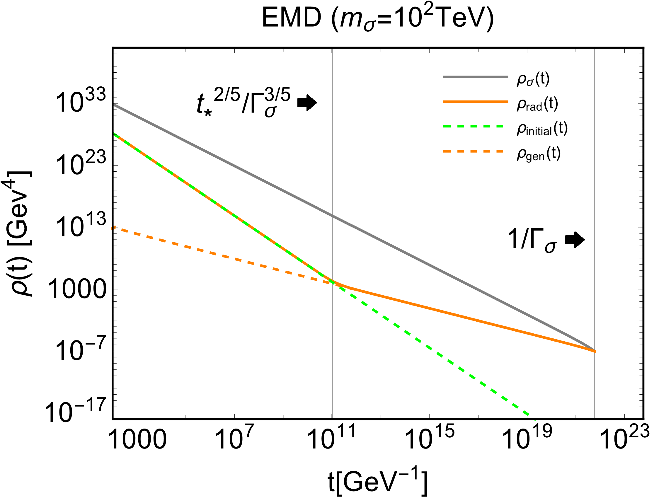
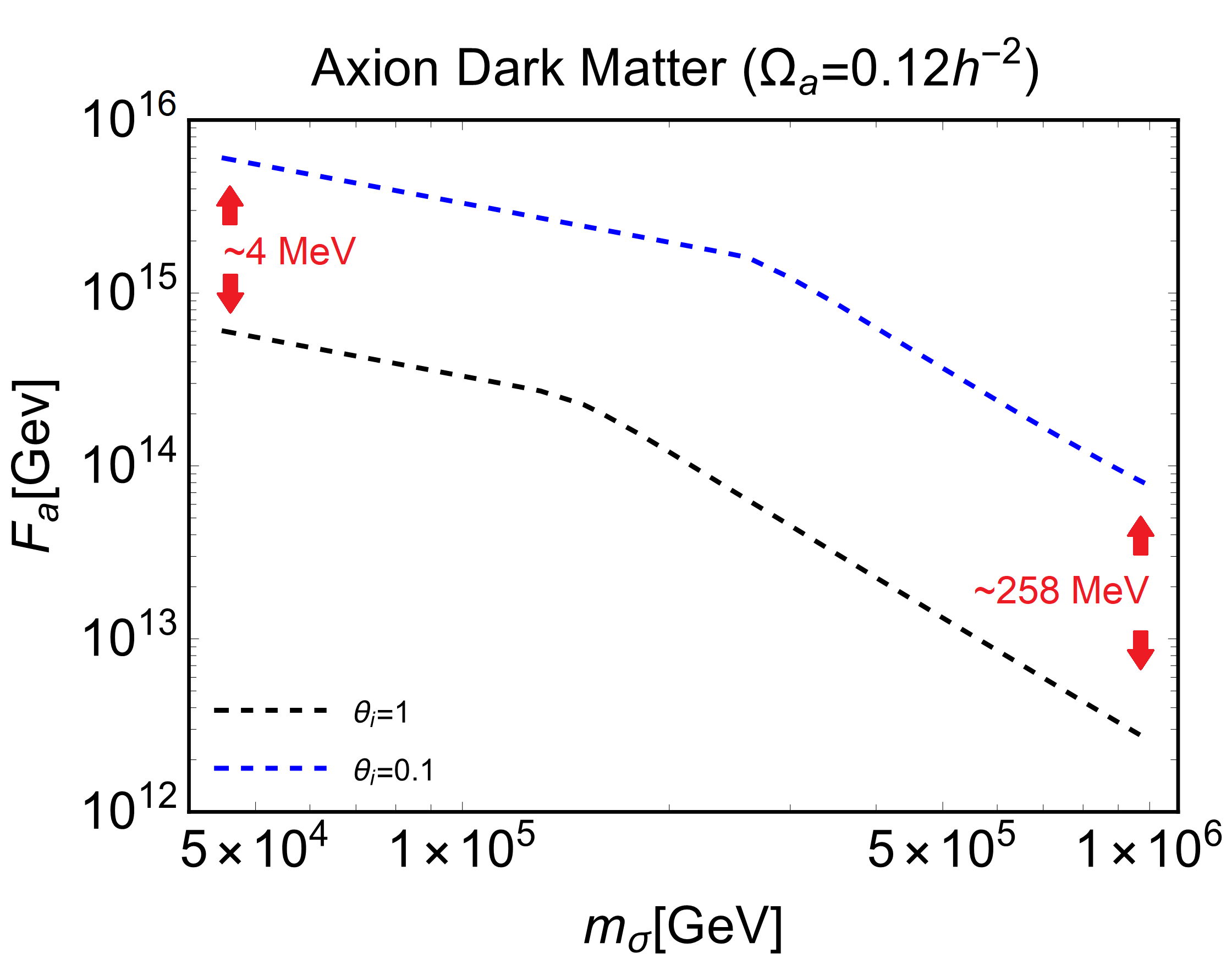
Figure 1: (Top) Evolution of energy densities of the heavy scalar $\displaystyle\sigma$ (gray solid) and the radiation (orange solid) during the EMD era with $\displaystyle m_{\sigma}=100\,\text{TeV}$, $\displaystyle\sigma_{0}=M_{p}$, and $\displaystyle t_{*}=8.715\times 10^{-6}$ ($\displaystyle{\rm GeV}^{-1}$). (Bottom) Values for the axion decay constant $\displaystyle F_{a}$ giving rise to $\displaystyle\Omega_{a}=0.12h^{-2}$ for a given heavy scalar mass $\displaystyle m_{\sigma}$ ($\displaystyle\sigma_{0}=M_{p}$). Blue (black) dashed line corresponds to the initial misalignment angle $\displaystyle\theta_{\rm i}=0.1$ (1). $\displaystyle T_{\rm rh2}$ associated with $\displaystyle m_{\sigma}=(45,10^{3})\,\text{TeV}$ are shown in red color.

where we used Eq. (91) and $\displaystyle t_{*}\sim 2/(3H(t_{*}))$.

We map the temperature of the thermal bath $\displaystyle T$ to the cosmological time $\displaystyle t$ via $\displaystyle\rho_{\text{rad}}(t)=(\pi^{2}/30)g_{*}(T)T^{4}$ with $\displaystyle g_{*}(T)$ the effective degrees of freedom of the energy density.

By using Eqs. (24) and (14), we obtain

$$\Omega_{a}h^{2}=\left(\frac{m_{a}(0)m_{a}(t_{\text{osc}})\theta_{\rm i}^{2}F_{a}^{2}}{2\rho_{\text{cr},0}h^{-2}}\right)\left(\frac{s_{0}\Delta^{-1}}{s_{\text{old}}(t_{\text{osc}})}\right)\,,$$ (32)

where $\displaystyle\rho_{\text{cr,0}}=1.053672\times 10^{-5}\,h^{2}\,\text{GeV/cm}^{3}$ and $\displaystyle s_{\rm old}(t_{\rm osc})$ can be written in terms of $\displaystyle s_{\rm old}(t_{\rm rh2})$ as

$$\displaystyle s_{\text{old}}(t_{\text{osc}}) \displaystyle=s_{\text{old}}(t_{\text{rh2}})\left(\frac{R_{\text{rh2}}}{R_{\text{osc}}}\right)^{3}\,,$$ (33)

$$\displaystyle=s_{\text{old}}(t_{\text{rh2}})\left(\frac{\rho_{\sigma}(t_{\text{osc}})}{\rho_{\sigma}(1/\Gamma_{\sigma})}e^{\Gamma_{\sigma}t_{\text{osc}}-1}\right)\,,$$ (34)

where we used the analytic solution of Eq. (25) and $\displaystyle s_{\text{old}}(t_{\text{rh2}})\propto\rho_{\text{initial}}^{3/4}(t_{\text{rh2}})$.

In the top panel of Fig. 1, we show the evolution of different energy densities during the EMD era characterized by $\displaystyle m_{\sigma}=100\,\text{TeV}$. The time estimate at which $\displaystyle\rho_{\text{initial}}(t_{\text{equal}})=\rho_{\text{gen}}(t_{\text{equal}})$ holds, i.e. $\displaystyle t_{\text{equal}}\,\approx\,t_{*}^{2/5}\Gamma_{\sigma}^{-3/5}$ agrees very well with the numerical result. Also, numerically the end of the EMD era can be found in Eq. (28) by requiring $\displaystyle\rho_{\sigma}(\Gamma_{\sigma}^{-1})\approx\rho_{\text{rad}}(\Gamma_{\sigma}^{-1})$. We confirmed that the numerically obtained $\displaystyle T_{\rm rh2}$ ($\displaystyle t_{\rm rh2}$) is in good agreement with the estimate below from $\displaystyle H(1/\Gamma_{\sigma})\approx\Gamma_{\sigma}$

$$T_{\text{rh2}}\approx 5\,\text{MeV}\left(\frac{10.75}{g_{*}(5\,\text{MeV})}\right)^{1/4}\left(\frac{m_{\sigma}}{45\,\text{TeV}}\right)^{3/2}\,.$$ (35)

The bottom panel of Fig. 1 shows values of $\displaystyle F_{a}$ enabling the axion to satisfy $\displaystyle\Omega_{a}h^{2}=0.12$ today for each given $\displaystyle m_{\sigma}$. In showing the relation obtained based on the numerical computation, we choose two particular values of the initial misalignment angle, $\displaystyle\theta_{\rm i}=1$ (black dashed line) and $\displaystyle\theta_{\rm i}=0.1$ (blue dashed line). Note that the entropy injection parametrized by $\displaystyle\Delta$ in Eq. (7) allows $\displaystyle F_{a}$ to reach larger values than those in the standard scenario for the shown range of $\displaystyle m_{\sigma}$. The break in both curves separates the region where the axion mass settles down to its zero temperature value from that where the axion mass is temperature-dependent, as shown in Eq. (20).

The reason for seeing such a $\displaystyle F_{a}$’s dependence on $\displaystyle m_{\sigma}$ in Fig. 1 is what follows. Assuming that $\displaystyle\sigma$-field starts oscillation at $\displaystyle t=t_{\rm rh1}$, we see that the ratio $\displaystyle\rho_{\sigma}(R_{\rm rh2})/s_{\rm old}(R_{\rm rh2})\propto T_{\rm rh1}$. Therefore, using the definition of $\displaystyle\Delta$ in Eq. (7), we obtain $\displaystyle\Delta\propto(T_{\rm rh1}/T_{\rm rh2})$ because of $\displaystyle\rho_{\sigma}(R_{\rm rh2})/s_{\rm new}(R_{\rm rh2})\propto T_{\rm rh2}$. Eventually combined with Eq. (35), $\displaystyle\Delta\propto T_{\rm rh2}^{-1}$ yields $\displaystyle\Delta\propto m_{\sigma}^{-3/2}$. Now that a larger $\displaystyle F_{a}$ requires a larger dilution factor $\displaystyle\Delta$ to be consistent with $\displaystyle\Omega_{a}h^{2}=0.12$ via Eqs. (1) and (2), it should correspond to a smaller $\displaystyle m_{\sigma}$, which is well reflected in Fig. 1.

IV Primordial Black Hole Formation

One of interesting possibilities resulting from the presence of the EMD era is formation of PBHs. For modes of the primordial fluctuation re-entering the horizon during the EMD era, if primordial fluctuations were large enough, these could possibly give rise to efficient formation of PBHs. As a matter of fact, indeed, the existing constraints on the power spectrum of the primordial curvature perturbation, $\displaystyle P_{\zeta}(k)$, for scales $\displaystyle k>10\,{\rm Mpc}^{-1}$ are not as strong as that Planck CMB data provides for $\displaystyle k\lesssim 0.2\,{\rm Mpc}^{-1}$.

Interests in PBH as a DM candidate have triggered many studies on ways to enhance the primordial perturbation on small scales. In the simplest minimal scenarios of the single field slow roll inflation, for instance, the presence of a small bump (or dip) Hertzberg and Yamada (2018); Mishra and Sahni (2020), and an inflection point in the inflaton potential Garcia-Bellido and Ruiz Morales (2017); Ballesteros and Taoso (2018); Kawasaki et al. (2016b); Germani and Prokopec (2017); Bhaumik and Jain (2020); Ballesteros et al. (2020a) can induce a peak in the small scale regime of the primordial power spectrum essentially through the ultra-slow roll at a late stage of inflation.

Assuming an inflaton potential featured by one of those, one may approximate $\displaystyle P_{\zeta}(k)$ on small scales as a lognormal form to get Gow et al. (2021); Bhattacharya et al. (2021)

$$\displaystyle P_{\zeta}(k) \displaystyle= \displaystyle A_{s}\left(\frac{k}{k_{\rm CMB}}\right)^{n_{s}-1}\,+\,A_{p}e^{-\frac{(N_{k}-N_{p})^{2}}{2\sigma_{p}^{2}}}$$ (36)

$$\displaystyle\simeq \displaystyle A_{s}\left(\frac{k}{k_{\rm CMB}}\right)^{n_{s}-1}\,+\,A_{p}e^{-\frac{(\log(k/k_{p}))^{2}}{2\sigma_{p}^{2}}}\,,$$ (38)

where $\displaystyle A_{s}=2.1\times 10^{-9}$, $\displaystyle n_{s}=0.965$, $\displaystyle k_{\rm CMB}=0.05\,{\rm Mpc}^{-1}$, and $\displaystyle N_{k}=\log(R(k)/R_{\rm end})$ and $\displaystyle N_{p}=\log(R(k_{p})/R_{\rm end})$ are defined. For the second equality, we used $\displaystyle H_{\rm inf}\simeq{\rm constant}$ during inflation, and $\displaystyle k=R(k)H_{\rm inf}$ and $\displaystyle k_{p}=R(k_{p})H_{\rm inf}$.

Once armed with such $\displaystyle P_{\zeta}(k)$ enhanced at small scales, the moduli-driven EMD era can serve as the environment facilitating formation of PBHs. Unlike in the radiation-dominated (RD) era, density fluctuations grow as $\displaystyle\delta\propto R$ in the matter-dominated era so as to reach the non-linear regime ($\displaystyle\delta=\mathcal{O}(1)$) rather quickly. This is basically due to the absence of the pressure preventing the gravitational collapse of an overdensity to a PBH during the matter-dominated era. With the PBH production probability defined as $\displaystyle\beta\equiv\rho_{\rm PBH}/\rho_{\rm tot}$ evaluated at the time of PBH formation, $\displaystyle\beta_{\rm MD}\simeq 0.056\,\sigma^{5}$ was obtained for $\displaystyle\sigma<0.01$ during the matter-dominated era with account taken of suppression in PBH production by the nonspherical effect Harada et al. (2016). Here $\displaystyle\sigma$ is the variance of the density fluctuation.

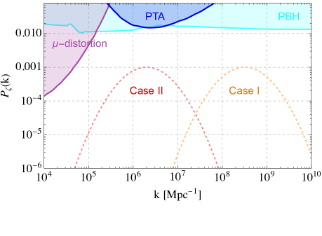
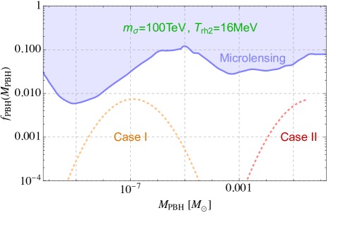
Figure 2: Top: The power spectra of the primordial curvature perturbation on small scales for the case I with $\displaystyle k_{p}=10^{8.5}{\rm Mpc}^{-1}$ (yellow) and the case II with $\displaystyle k_{p}=2\times 10^{6}{\rm Mpc}^{-1}$ (red). Also $\displaystyle A_{p}=10^{-3}$ and $\displaystyle\sigma_{p}=1$ are commonly assumed. We showed the various constraints on $\displaystyle P_{\zeta}(k)$ based on PBH abundance, Pulsar timing array (PTA) and $\displaystyle\mu$-distortion of CMB energy spectrum with the cyan, blue and purple shaded regions respectively. Bottom: The fraction of DM in PBH which was formed during the EMD era and resulted from $\displaystyle P_{\zeta}(k)$ shown in the left panel. The assumed example $\displaystyle m_{\sigma}$ and $\displaystyle T_{\rm rh2}$ is specified in the top with the green color. The light blue shaded region is the constraint on $\displaystyle f_{\rm PBH}$ based on the microlensing.

The fraction of PBH with a mass $\displaystyle M$ in DM ($\displaystyle f_{\rm PBH}(M)=\rho_{\rm PBH,0}/\rho_{\rm DM,0}$) can be read from the mass function which reads

$$\displaystyle\psi(M) \displaystyle\simeq \displaystyle\frac{1}{M}\frac{\rho_{\rm PBH,0}(M)}{\rho_{\rm DM,0}}$$ (39)

$$\displaystyle= \displaystyle\frac{1}{M}\frac{\rho_{\rm PBH,0}(M)}{\rho_{\rm m,0}}\frac{\rho_{\rm m,0}}{\rho_{\rm DM,0}}$$ (41)

$$\displaystyle= \displaystyle\frac{1}{M}\frac{\rho_{\rm PBH,eq}(M)}{\rho_{\rm m,eq}}\frac{\Omega_{\rm m,0}h^{2}}{\Omega_{\rm DM,0}h^{2}}$$ (43)

$$\displaystyle= \displaystyle\frac{1}{M}\frac{\rho_{\rm PBH,eq}(M)}{\rho_{\rm rad,eq}}\frac{\Omega_{\rm m,0}h^{2}}{\Omega_{\rm DM,0}h^{2}}$$ (45)

$$\displaystyle= \displaystyle\frac{\Omega_{\rm m,0}h^{2}}{\Omega_{\rm DM,0}h^{2}}\frac{\beta_{\rm MD}(M)}{M}\frac{R_{\rm eq}}{R_{\rm rh2}}$$ (47)

$$\displaystyle= \displaystyle 4.88\times 10^{27}\times\frac{\beta_{\rm MD}(M)}{M}\sqrt{\frac{\Gamma_{\sigma}}{M_{P}}}\,,$$ (49)

where $\displaystyle R_{\rm eq}/R_{\rm rh2}=\sqrt{H_{\rm rh2}/H_{\rm eq}}$, $\displaystyle H_{\rm rh2}=\Gamma_{\sigma}$, $\displaystyle\Omega_{\rm m,0}=0.315$, $\displaystyle\Omega_{\rm DM,0}=0.265$ Aghanim et al. (2020), $\displaystyle g_{*}(R_{\rm eq})=3.36$ and $\displaystyle T_{\rm eq}\simeq 0.75{\rm eV}$ were used for the last equality with $\displaystyle R_{\rm eq}$ ($\displaystyle R_{\rm rh2}$) the scale factor at the matter-radiation equality (the time of the moduli decay). In obtaining the third and fifth equalities, the scaling behaviors $\displaystyle\rho_{\rm PBH}\propto R^{-3}$ and $\displaystyle\rho_{\rm rad}\propto R^{-4}$ were used for PBH and radiation.

In combination with $\displaystyle\beta_{\rm MD}\simeq 0.056\sigma^{5}$ and Eq. (6), Eq. (49) leads on to

$$f_{\rm PBH}(M)\simeq(2.35\times 10^{5})\times P_{\zeta}(k)^{5/2}\times\left(\frac{m_{\sigma}}{100{\rm TeV}}\right)^{3/2}\,.$$ (50)

where $\displaystyle M$-dependence of $\displaystyle f_{\rm PBH}$ is realized via $\displaystyle k$ dependence of $\displaystyle P_{\zeta}(k)$ on the RHS and the approximate relation $\displaystyle\sigma(M)\approx 2(1+w)(5+3w)^{-1}\sqrt{P_{\zeta}(k)}$ was used with $\displaystyle w=0$. The mapping between $\displaystyle k$ and $\displaystyle M$ can be found in Eq. (LABEL:eq:MPBH). In the scenario of our interest, DM population consists of axion and PBH, and thus the sum of the relic abundances of the two amounts to that of DM, i.e.

$$\Omega_{\text{DM}}=\Omega_{a}(m_{\sigma},F_{a})+\Omega_{\text{PBH}}(m_{\sigma},F_{a},P_{\zeta})\,.$$ (52)

where

$$\Omega_{\text{PBH}}=\Omega_{\text{DM}}\times\int\text{d}\,\text{ln}M\,f_{\text{PBH}}(M)\,,$$ (53)

In the top panel of Fig. 2, we first show the exemplary primordial power spectrum assumed for the case I (yellow dashed) and II (red dashed). The region above the cyan, blue and purple lines are excluded by constraints from PBH abundance, Pulsar timing array (PTA) and $\displaystyle\mu$-distortion of CMB energy spectrum Gow et al. (2021) respectively. In conversion of the constraints on the associated observational quantities to $\displaystyle P_{\zeta}(k)$, $\displaystyle\sigma_{p}=1$ was assumed in Eq. (38). One can safely assume $\displaystyle P_{\zeta}(k)$ as large as $\displaystyle\mathcal{O}(10^{-3})$ for $\displaystyle k>10^{5}{\rm Mpc}^{-1}$ to achieve $\displaystyle f_{\rm PBH}$ as desired in the presence of the EMD era. For the case I and II specified in the introduction, we take the exemplary lognormal power spectrum on small scales with $\displaystyle A_{p}=10^{-3}$ and $\displaystyle\sigma_{p}=1$ for both, and $\displaystyle k_{p}=10^{8.5}{\rm Mpc}^{-1}$ (case I) and $\displaystyle 2\times 10^{6}{\rm Mpc}^{-1}$ (case II).

Particularly, the constraint on $\displaystyle P_{\zeta}(k)$ from PTA is based on NANOGrav 11 year data. We note that the future sensitivity of measurement of $\displaystyle\Omega_{\rm GW}h^{2}$ by SKA can be several orders of magnitude better than NANOGrav, which allows for SKA to probe $\displaystyle P_{\zeta}(k)=\mathcal{O}(10^{-5})$. Interestingly, as will be discussed in Sec. VII, the same radio telescope SKA can detect the radio signals from the encounter between UCMH and neutron star. Therefore, we expect that probing the stochastic GW background induced by the enhanced $\displaystyle P_{\zeta}(k)$ we assumed in the case II by SKA can be the complementary way of testing our scenario to the radio signal search by SKA. Null observation of either the stochastic GW background at the frequency range corresponding to the case II or radio signal by SKA will potentially exclude or support the case II.

As a result of the assumed $\displaystyle P_{\zeta}(k)$’s in the top panel, there arise PBHs during the EMD era contributing to the DM energy density by $\displaystyle f_{\rm PBH}$ in Eq. (50) as shown in the bottom panel of Fig. 2. The $\displaystyle k$-modes re-entering the horizon at $\displaystyle t_{*}$ and at $\displaystyle t_{\rm max}$ determine the minimum ($\displaystyle M_{\rm min}$) and maximum ($\displaystyle M_{\rm max}$) PBH masses formed during the EMD era. $\displaystyle t_{\rm max}$ is defined to be the horizon re-entry time of $\displaystyle k_{\rm max}$ of which associated fluctuation grows to 1 at $\displaystyle t_{\rm rh2}$. $\displaystyle k_{\rm min}$ and $\displaystyle k_{\rm max}$ are computed in Eq. (LABEL:eq:kmin2) and (109), providing $\displaystyle M_{\rm min}$ and $\displaystyle M_{\rm max}$ when plugged in Eq. (LABEL:eq:MPBH). For instance, for $\displaystyle m_{\sigma}=100{\rm TeV}$ and $\displaystyle T_{\rm rh2}=16{\rm MeV}$, we find $\displaystyle M_{\rm max}\simeq 3\times 10^{-3}M_{\odot}$ and $\displaystyle 0.3M_{\odot}$ for the case I and II, respectively.

For the case II, $\displaystyle k_{p}\simeq k_{\rm max}$ is observed so that the peak in $\displaystyle f_{\rm PBH}$ contour is cut near $\displaystyle M_{\rm max}$ as far as PBH generated during the EMD era is concerned. In contrast, for the case I, since $\displaystyle k_{\rm max}\simeq 10^{7}{\rm Mpc}$ is more than one order of magnitude smaller than $\displaystyle k_{p}=10^{8.5}{\rm Mpc}^{-1}$, the cut near the peak does not take place. Note that for $\displaystyle\sigma\lesssim 0.005$, $\displaystyle\beta_{\rm MD}\simeq 0.056\sigma^{5}$ does not hold because $\displaystyle\beta_{\rm MD}$ needs modified to encode the effect of the collapsing region’s angular momentum (spin of PBH) Harada et al. (2017). The bottom panel of Fig. 2 reflects the region of $\displaystyle k$ satisfying $\displaystyle\sigma>0.005$.

For the assumed $\displaystyle P_{\zeta}(k)$, we have seen that $\displaystyle f_{\rm PBH}\simeq 10^{-2}$ can be indeed achieved for the PBH mass ranges that each case is targeting via Fig. 2. Thus the relatively weak current constraints on $\displaystyle P_{\zeta}(k)$ on small scales and UV-physics motivated EMD era can be interesting points to motivate one to think about $\displaystyle f_{\rm PBH}\lesssim\mathcal{O}(10^{-2})$ for $\displaystyle M_{\rm PBH}$ specified in Fig. 2. Bearing in mind this possibility for PBH as a minor component of DM and the underlying physics for PBH formation in the early universe, in the coming sections we study interesting astrophysical phenomenology caused by PBHs with $\displaystyle f_{\rm PBH}=\mathcal{O}(10^{-2})$. Particularly since the axion is the major component of DM in our scenario, our study concerns physics resulting from the interplay between the axion and PBH.

V UCMH formation

The PBH formation via an EMD era could potentially play an important role in axion searches. A dark halo is predicted to form around an isolated and stationary PBH during the late time matter domination era via secondary infall accretion. Such an accretion leads to the formation of the so-called ultracompact minihalos (UCMHs) as shown in  Bertschinger (1985); Mack et al. (2007). The growth in the mass and the radius of UCMH in time (parametrized by the redshift $\displaystyle z$) can be seen from  Mack et al. (2007); Berezinsky et al. (2013); Ricotti and Gould (2009)

$$\displaystyle M_{\text{UCMH}}(z) \displaystyle=3\left(\frac{1000}{1+z}\right)\,M_{\text{PBH}}\,,$$ (54)

$$\displaystyle R_{\text{UCMH}}(z) \displaystyle=0.019\,\text{pc}\left(\frac{1000}{z+1}\right)\left(\frac{M_{\text{UCMH}}(z)}{M_{\odot}}\right)^{1/3}\,.$$ (55)

The growth eventually leads to the formation of the steep radial density profile of the following form Ricotti and Gould (2009); Bringmann et al. (2012)

under the approximation $\displaystyle\Omega_{\text{DM}}/\Omega_{m}\approx 1$.

This profile indeed was confirmed by the first N-body simulation of the universe composed of a smooth DM particle background plus a small fraction of PBHs Adamek et al. (2019). The growth of UCMHs stops when they begin to interact with non-linear structures at around $\displaystyle(z\sim 30-10)$ Berezinsky et al. (2013), so that the UCMH abundance is given by $\displaystyle f_{\text{UCMH}}\sim 10^{2}f_{\text{PBH}}$, where $\displaystyle f_{\text{PBH}}$ is the original fraction of DM in naked PBHs. The above equations only holds for $\displaystyle f_{\text{PBH}}\lesssim 10^{-2}$ to ensure the isolated assumption.

The most inner region of the UCMH is softened by angular momentum conservation as was pointed out in Bringmann et al. (2012) and previous works take a conservative approach to model the inner region with a cut-off within which one takes the UCMH density to be nearly constant (see, for example,  Li et al. (2012)) . Here we use the simplified version for UCMH density given in Eq. (55) (for completeness, we have added in Appendix C the density profile including an inner core).

VI Axion Direct Detection via Tidal Streams (CASE I)

In this section, we consider $\displaystyle f_{\rm PBH}=\mathcal{O}(10^{-2})$ with $\displaystyle M_{\rm PBH}\lesssim\mathcal{O}(10^{-6})M_{\odot}$, which corresponds to the case I. The formation of tidal streams from disruption of axion miniclusters during their encounters with stars in the local neighborhood as well as its implication for axion direct searches was discussed in Tinyakov et al. (2016). The key idea is that such tidal streams may still hold densities larger than the average. In the context of axion searches, the stream-crossing events would hold a reasonable rate of about $\displaystyle 1/20\,\text{yr}^{-1}$, leading to a signal amplification in axion detectors by a factor $\displaystyle\sim 10$ during 2-3 days.

In this section, we apply the above idea to UCMHs that possibly get generated for the case I in Fig. 2 (right panel). It is well known that UCMHs seeded by solar mass PBHs are extremely resistant against disruption from high speed encounters with stars. The reason is the following. The critical impact parameter, i.e. the impact parameter between the star and the UCMH which leads to a total UCMH disruption (or at least a significant loss of mass), is much shorter than the typical UCMH radius. Only encounters with very small impact parameters in terms of the UCMH radius will lead to one-off disruption. Since such encounters are statistically disfavored, the disruption of UCMHs due to encounters with stars at the solar neighborhood is negligible. However, when it comes to PBH seeds with much lighter masses, the situation changes.

The critical impact parameter $\displaystyle b_{c}$ is defined as $\displaystyle\Delta E(b_{c})=E_{b}$ with $\displaystyle\Delta E$ the UCMH internal energy obtained after the encounter with a star and $\displaystyle|E_{b}|$ its binding energy. For impact parameters satisfying $\displaystyle b\lesssim R_{\rm UCMH}$, the distant-tide approximation is no longer valid. Thus, it becomes necessary to use the following parametrization performed in Carr and Sakellariadou (1999) which is valid in both $\displaystyle b\ll R_{\text{UCMH}}$ and $\displaystyle b\gg R_{\text{UCMH}}$ regimes Hertzberg et al. (2020a)

$$\displaystyle\Delta E_{\gg\ll}\approx\frac{16\pi}{3}\left(\frac{G_{N}M_{\star}}{v_{\textrm{rel}}b^{2}}\right)^{2}\times$$

$$\displaystyle\int_{0}^{R_{\textrm{UCMH}}}dr\,r^{4}\rho_{\textrm{UCMH}}(r)\left(1+\frac{4r^{4}}{9b^{4}}\right)\left(1+\frac{2r^{2}}{3b^{2}}\right)^{-4}\,,$$ (57)

$$\displaystyle\approx 6.5\times 10^{-21}\,M_{\odot}\left(\frac{M_{\star}}{M_{\odot}}\right)^{2}\left(\frac{220\,\textrm{km/s}}{v_{\textrm{rel}}}\right)^{2}\left(\frac{R_{\textrm{UCMH}}}{b}\right)^{2}\times$$

$$\displaystyle\left(\frac{M_{\textrm{PBH}}}{M_{\odot}}\right)^{1/3}\left(\frac{10^{2}\,M_{\textrm{PBH}}}{M_{\textrm{UCMH}}}\right)^{5/3}\left[\frac{S(R_{\textrm{UCMH}}/b)}{S(1)}\right]\,,$$ (58)

where $\displaystyle M_{\star}$ is the mass of the encountered star, $\displaystyle S(1)=0.066$ and

$$S(R_{\textrm{UCMH}}/b)=\sum_{i=1}^{4}C_{i}\,{}_{2}F_{1}\left[\frac{3}{8},i,\frac{11}{8},-\frac{2}{3}\left(\frac{R_{\textrm{UCMH}}}{b}\right)^{2}\right]\,,$$

with $\displaystyle\left\{C_{i}\right\}_{i=1}^{4}=(1,-3,4,-2)$ and ${}_{2}F_{1}$ is the known Gauss hypergeometric function.

On the other hand, the UCMH binding energy is given by

$$E_{b}\approx 2.4\times 10^{-10}\,M_{\odot}\left(\frac{M_{\textrm{UCMH}}}{10^{2}\,M_{\textrm{PBH}}}\right)^{2/3}\left(\frac{M_{\textrm{PBH}}}{M_{\odot}}\right)^{5/3}\,.$$ (59)

The critical impact parameter can then be obtained by solving numerically $\displaystyle\Delta E(b_{c})=E_{b}$ with the use of Eqs. (58) and (59).

In the regime $\displaystyle b\ll R_{\text{UCMH}}$, we can expand $\displaystyle S(R_{\textrm{UCMH}}/b)$ of Eq. (58) in a Taylor series at around $\displaystyle b/R_{\textrm{UCMH}}=0$ to obtain Hertzberg et al. (2020a)

$$\displaystyle\frac{b_{c}}{R_{\textrm{UCMH}}}\approx 1.5\times 10^{-8}\left(\frac{M_{\star}}{M_{\odot}}\right)^{8/5}\times$$

$$\displaystyle\left(\frac{220\,\frac{km}{s}}{v_{\textrm{rel}}}\right)^{8/5}\left(\frac{M_{\odot}}{M_{\textrm{PBH}}}\right)^{16/15}\left(\frac{10^{2}\,M_{\textrm{PBH}}}{M_{\textrm{UCMH}}}\right)^{28/15}\,.$$ (60)

In the other regime $\displaystyle b\gg R_{\text{UCMH}}$, we can expand Eq. (57) around $\displaystyle(r/b)=0$. We see that the expression for the gained internal energy asymptotically approaches the well-known distant-tide approximation when $\displaystyle b/R_{\textrm{halo}}\rightarrow\infty$ Binney and Tremaine (2008); Spitzer (1958), i.e.

$$\Delta E_{\gg}\approx\frac{4\langle r^{2}\rangle}{3}\frac{G_{N}^{2}M_{\star}^{2}M_{\textrm{UCMH}}}{v_{\textrm{rel}}^{2}b^{4}}\,,$$ (61)

where

$$\langle r^{2}\rangle=\left(\frac{1}{M_{\textrm{UCMH}}}\right)\int^{R_{\text{UCMH}}}d^{3}r\,r^{2}\rho_{\textrm{UCMH}}(r)$$ (62)

is the mass-weighted mean-square UCMH radius.

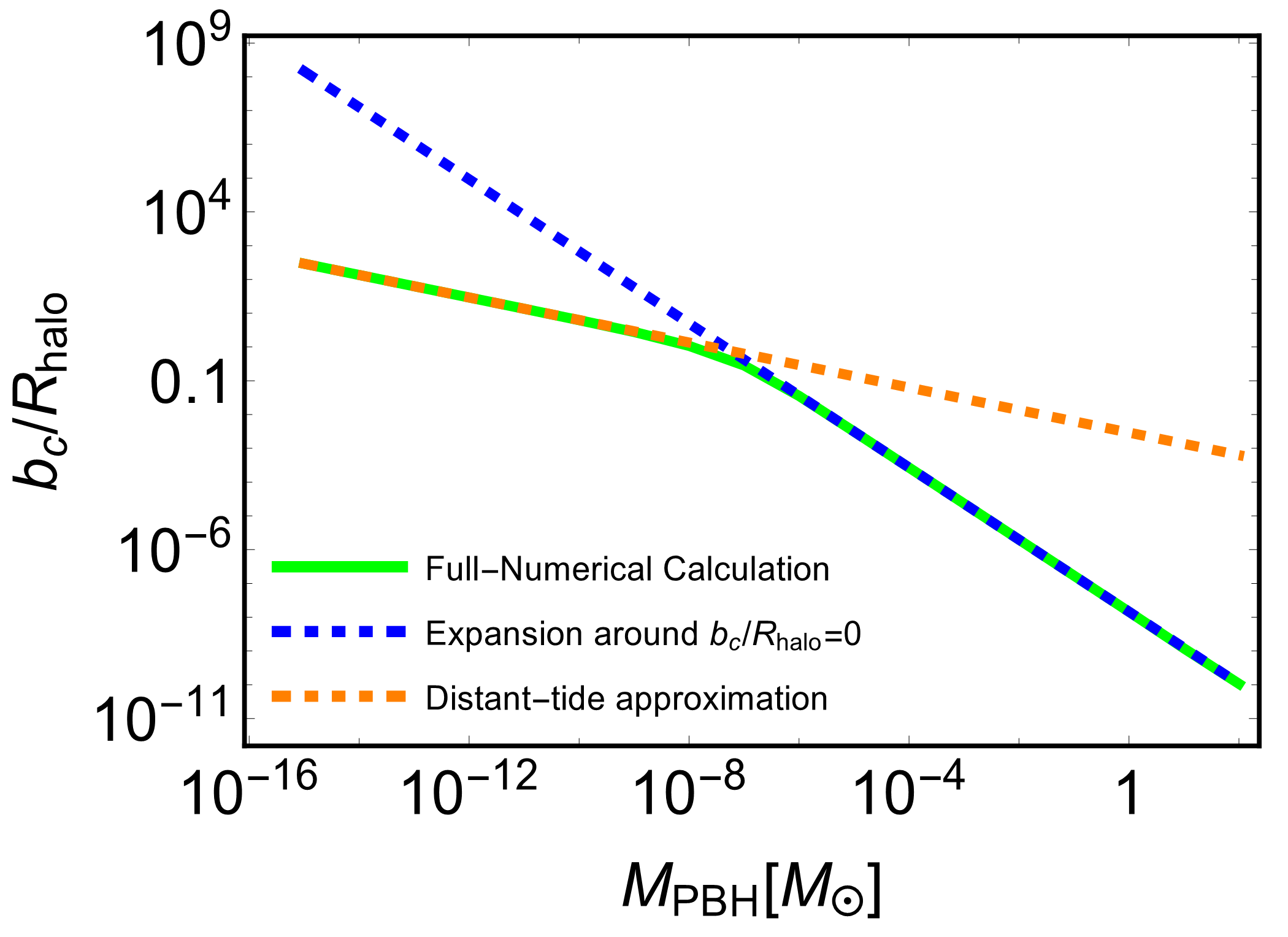
Figure 3: Critical impact parameter normalized by the UCMH radius using a full numerical calculation (solid green line), an expansion around $\displaystyle b_{c}/R_{\text{UCMH}}=0$ (dashed blue line), and the distant-tide approximation (dashed orange line). We have fixed $\displaystyle M_{\text{UCMH}}=10^{2}\,M_{\text{PBH}}$ and $\displaystyle v_{\text{rel}}=220\,\text{km/s}$.

In Fig. 3, we show the result of the full numerical calculation for the critical impact parameter (solid green line) together with the approximation given in Eq. (60) valid for $\displaystyle b\ll R_{\text{UCMH}}$ (dashed blue line) and the distant-tide approximation valid for $\displaystyle b\gg R_{\text{UCMH}}$ (dashed orange line). We see that there is a clear break in the curve at around $\displaystyle M_{\text{PBH}}\sim\mathcal{O}(10^{-8})\,M_{\odot}$, which separates the regimes in which the critical impact parameter is larger or smaller than the UCMH radius. For $\displaystyle M_{\text{PBH}}\lesssim 10^{-8}\,M_{\odot}$, the critical impact parameter is well-described under the distant-tide approximation.

Consider a star field with a density $\displaystyle n_{\star}$ and suppose that the minicluster spends a time $\displaystyle t_{\text{cross}}$ within such a field. With account taken of the sum of one-off disruptive events with $\displaystyle b<b_{c}$ and the contribution from multiple encounters with $\displaystyle b\geq b_{c}$, the UCMH disruption probability during one-single crossing ($\displaystyle P_{s}$) through the galactic disk reads Schneider et al. (2010),

$$\displaystyle P_{s} \displaystyle=2\pi n_{\star}v_{\text{rel}}t_{\text{cross}}\times\left(\int_{0}^{b_{c}}bdb+\frac{1}{E_{b}}\int_{b_{c}}^{\infty}\Delta E(b)bdb\right)\,,$$ (63)

$$\displaystyle=\left(\frac{\pi b_{c}^{2}}{M_{\star}}\right)\times S_{\perp}+\frac{2\pi}{M_{\star}}\left(\frac{1}{E_{b}}\int_{b_{c}}^{\infty}\Delta E(b)bdb\right)\times S_{\perp}\,,$$ (64)

where we took the field as a column of stars with density $\displaystyle n_{\star}$ and height $\displaystyle H$, so that the (perpendicular) crossing time is $\displaystyle t_{\text{cross}}=H/v_{\text{rel}}$ and $\displaystyle n_{\star}=S_{\perp}/(HM_{\star})$ with $\displaystyle S_{\perp}\approx 35\,M_{\odot}\text{pc}^{-2}$ Kuijken and Gilmore (1989) the perpendicular surface mass density in the local neighborhood. By assuming isotropically distributed trajectories and setting the maximum trajectory length to be no longer than $\displaystyle\mathcal{O}(10)$ kpc to avoid a logarithmic divergence in the angular integration, authors in Tinyakov et al. (2016) shows that the probability $\displaystyle P_{s}$ in Eq. (64) needs to be re-scaled as $\displaystyle P_{s}\rightarrow 4P_{s}$ to include different directions.

To estimate the total probability for UCMH disruption, $\displaystyle P_{\text{Total}}$, we multiply the disruption probability during a single disk crossing by the total number of crossings during the age of the Milky Way $\displaystyle T_{\text{MW}}\sim 10\,\text{Gyr}$, $\displaystyle N_{\text{cross}}\sim 100$. Since $\displaystyle P_{\text{Total}}=P_{\text{Total}}(t)$ by construction, a total probability equal to one means that a time $\displaystyle t=T_{\text{MW}}$ is needed to disrupt all UCMHs. A $\displaystyle P_{\text{Total}}>1$ means that such a total disruption occurs during a total time $\displaystyle t<T_{\text{MW}}$.

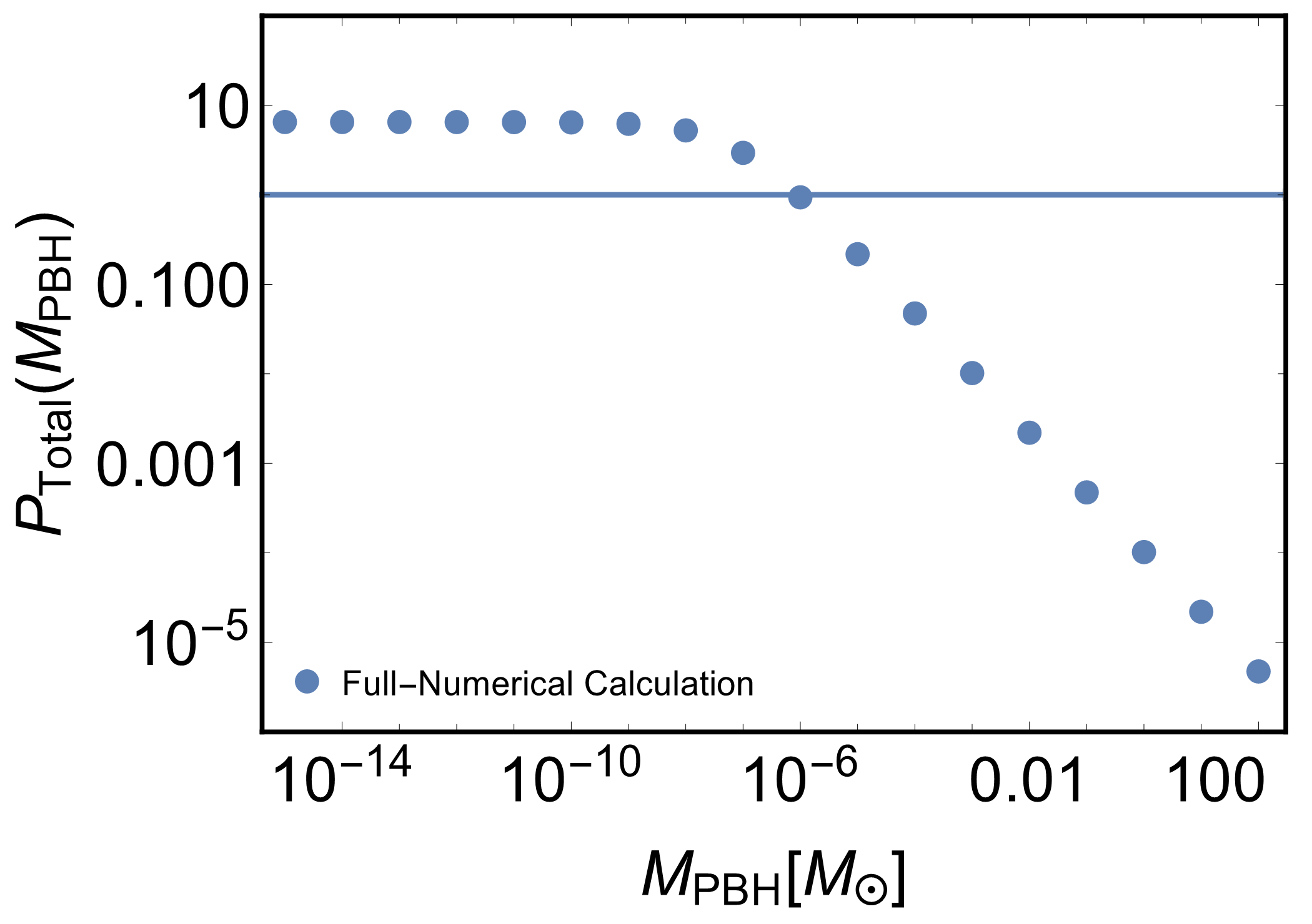
Figure 4: Probability of UCMH disruption in the local neighborhood using a full numerical calculation (blue points). We have fixed $\displaystyle M_{\text{UCMH}}=10^{2}\,M_{\text{PBH}}$ and $\displaystyle v_{\text{rel}}=220\,\text{km/s}$. The blue line indicates $\displaystyle P_{\text{Total}}=1$.

Fig. 4 shows the total disruption probability of UCMHs in the local neighborhood based on Eq. (64). We have used $\displaystyle M_{\text{UCMH}}=10^{2}\,M_{\text{PBH}}$ and $\displaystyle v_{\text{rel}}=220\,\text{km/s}$. We see that all UCMHs are disrupted for $\displaystyle M_{\text{PBH}}\lesssim 10^{-6}M_{\odot}$. Such a phenomenon could potentially have a great impact on axion direct searches.

On disruption of UCMHs, debris arise, which become tidal streams along the UCMH path. For orbits with small ellipticity, the streams can be considered to be one-dimensional structures of a length $\displaystyle L_{st}$ and a cross-section $\displaystyle\sim\mathcal{O}(R_{\text{UCMH}}^{2})$. Such a tidal stream formation process was modeled in Schneider et al. (2010); Angus and Zhao (2007) for DM clumps with a mass $\displaystyle\sim 10^{-6}M_{\odot}$. Here we closely follow  Schneider et al. (2010); Tinyakov et al. (2016) to estimate the typical length of tidal streams $\displaystyle L_{\text{st}}\sim\sigma_{a}\Delta t$ with $\displaystyle\sigma_{a}$ the axion velocity dispersion of the initial UCMH, and $\displaystyle\Delta t$ the time between UCMH disruption and today. Under this approximation, the UCMH grows in volume by a factor $\displaystyle\sigma_{a}\Delta t/R_{\text{UCMH}}$ during a time period $\displaystyle\Delta t$. This gives rise to dilution of the UCMH radial density in a plane perpendicular to the stream axis

$$\displaystyle\rho_{\text{st}}(r)=\rho_{\text{UCMH}}(r)\times\frac{r}{\sigma_{a}(r)\Delta t}\,,\,$$ (65)

$$\displaystyle\approx 0.06\,M_{\odot}\text{pc}^{-3}\left(\frac{10^{-2}}{r/R_{\text{UCMH}}}\right)^{9/8}\left(\frac{10^{2}\,M_{\text{PBH}}}{M_{\text{UCMH}}}\right)^{3/2}\,,$$ (66)

where $\displaystyle\sigma_{a}(r)=(0.3\,G_{N}M_{\text{UCMH}}(r)/r)^{1/2}$ as obtained in Appendix D via the corresponding ergodic distribution function of the UCMH. To obtain a conservative estimate, we have used $\displaystyle\Delta t=10\,\text{Gyr}$. Given the local DM density $\displaystyle\rho_{\text{local}}=0.008\pm 0.003\,M_{\odot}\text{pc}^{-3}$ Bovy and Tremaine (2012), it is realized that tidal streams can reach densities about an order of magnitude larger than $\displaystyle\rho_{\text{local}}$ in its inner region at $\displaystyle r\simeq 10^{-2}R_{\text{UCMH}}$.

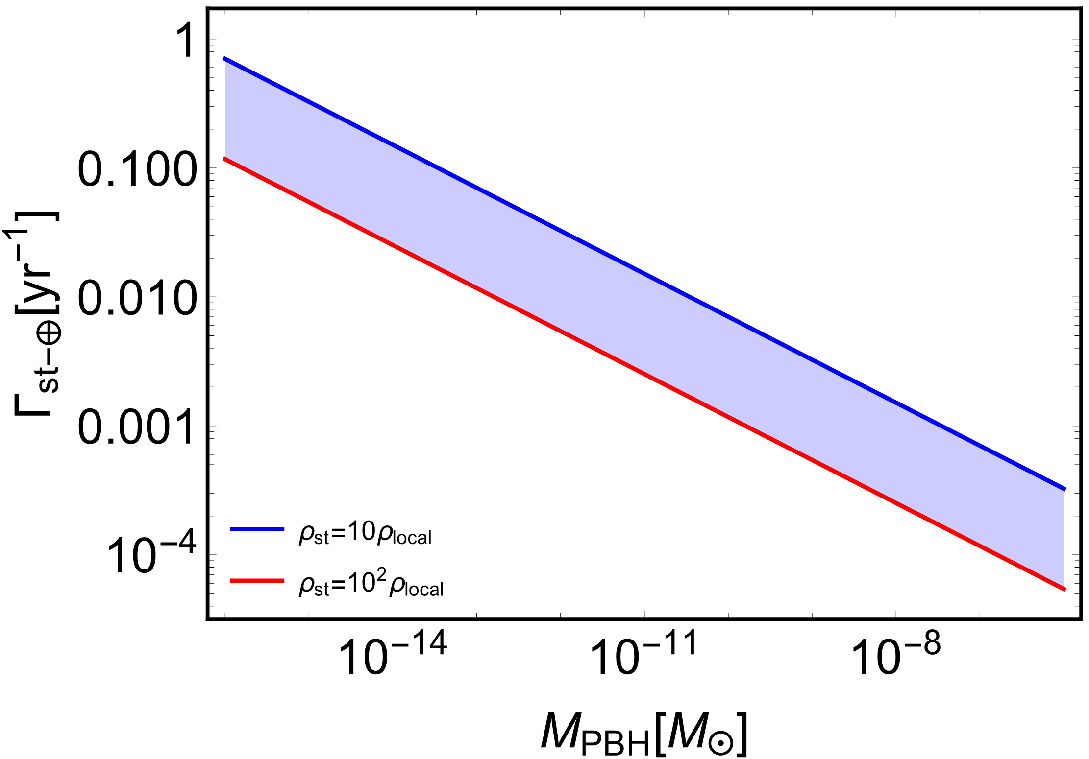
Figure 5: Earth and tidal stream encounter rate for UCMHs in terms of the central PBH mass according to Eq. (69). We have taken $\displaystyle M_{\text{UCMH}}=10^{2}\,M_{\text{PBH}}$ as the original UCMH mass.

The probability that the Earth passes by one of tidal streams is expected to be proportional to the total number of UCMH within a certain volume, namely the filling factor. Given that for $\displaystyle M_{\text{PBH}}\lesssim 10^{-6}\,M_{\odot}$, the local number density of tidal streams is equal to the initial PBH number densities, i.e. $\displaystyle n_{\text{st}}=n_{\text{PBH}}$, the filling factor (FF) reads

$$\displaystyle\text{FF(r)}=\left(\frac{f_{\text{PBH}}\rho_{\text{local}}}{M_{\text{PBH}}}\right)\times\left(\frac{4\pi r^{3}}{3}\frac{\sigma_{a}(r)\Delta t}{r}\right)\,,$$ (67)

$$\displaystyle\approx 0.001\left(\frac{f_{\text{PBH}}}{10^{-2}}\right)\left(\frac{r/R_{\text{UCMH}}}{10^{-2}}\right)^{15/8}\left(\frac{M_{\text{UCMH}}}{10^{2}\,M_{\text{PBH}}}\right)^{5/2}\,.$$ (68)

Using Eq. (68), we estimate the Earth-tidal stream encounter rate as

$$\Gamma_{{\rm st}-\oplus}(r)=\frac{\text{FF}(r)}{\tau(r)}=\text{FF}(r)\times\frac{v_{\text{rel}}}{2r}\,,$$ (69)

where

Here $\displaystyle\tau(r)$ is the typical crossing time of the Earth through a high dense DM zone of radius $\displaystyle r$ within the tidal stream. We are assuming that Earth is crossing such a tidal perpendicularly to its axis.

Thinking of DM direct searches, we require that such a high axion zone holds a density $\displaystyle\rho_{\text{st}}\in[10-100]\rho_{\text{local}}$ to calculate in Figure 5 the Earth-tidal stream encounter rate in terms of the central PBH mass. One can see that the lighter the central PBH in (undisrupted) UCMHs is, the larger the encounter rate for fixed $\displaystyle\rho_{\text{st}}$ becomes. Interestingly, $\displaystyle\Gamma_{{\rm st}-\oplus}$ can be high enough so that the Earth can encounter the tidal stream of axion DM with the enhanced $\displaystyle\rho_{\text{st}}\gtrsim 10\rho_{\text{local}}$ once every (1-10) years for $\displaystyle M_{\text{PBH}}\lesssim 10^{-14}M_{\odot}$, which is comparable to that found in Tinyakov et al. (2016) for the case of axion miniclusters.

If the aforementioned scenario becomes the case, one can expect the significantly enhanced chance for direct search experiments on the Earth to detect axion with the decay constant $\displaystyle F_{a}\gtrsim 10^{12}\,\text{GeV}$) (see the bottom panel in Fig. 1). We notice that the future planned ABRACADABRA Kahn et al. (2016) experiment can probe $\displaystyle g_{a\gamma\gamma}-m_{a}$ parameter space that the scenario of our interest indicates.

The coupling of axion to photon via the operator $\displaystyle\mathcal{L}=-(g_{a\gamma\gamma}/4)aF^{\mu\nu}\tilde{F}_{\mu\nu}$ modifies the Maxwell equations so that there arises an axion-sourced effective current $\displaystyle\vec{J}_{a}(t)$ in the presence of a static magnetic field background $\displaystyle\vec{B}_{0}$. Given $\displaystyle a=(\sqrt{2\rho_{\rm DM}}/m_{a})\sin(m_{a}t)$, the oscillating $\displaystyle\vec{J}_{a}(t)$ induces the real oscillating magnetic field with frequency $\displaystyle m_{a}$ of which flux through the pick-up loop reads

$$\Phi_{a}(t)=g_{a\gamma\gamma}|\vec{B}_{0}|\sqrt{2\bar{\rho}_{a}}\text{cos}(m_{a}t)\,,$$ (71)

where $\displaystyle\bar{\rho}_{a}$ is the axion background energy density.

In light of our scenario, we expect there can be two interesting effects on the experiment. Firstly, for the case where the experimental sensitivity is still not good enough to probe ($\displaystyle g_{a\gamma\gamma}$,$\displaystyle m_{a}$), we expect a temporary improvement of the experimental sensitivity on the earth’s encountering the tidal stream with $\displaystyle\bar{\rho}_{\text{st}}$. For a given experimental set-up characterized by the magnitude of the external magnetic field and volume containing it, i.e. ($\displaystyle B_{0,{\rm max}},V_{\rm B}$), what matters in the flux in Eq. (71) is the product $\displaystyle g_{a\gamma\gamma}\sqrt{\bar{\rho}_{a}}$. This means that when there is an enhancement in $\displaystyle\bar{\rho}_{a}$ due to the earth’s encountering the tidal stream with $\displaystyle\bar{\rho}_{\text{st}}$, the experimental sensitivity for $\displaystyle g_{a\gamma\gamma}$ increases by

$$g_{a\gamma\gamma}=g_{a\gamma\gamma}(\bar{\rho}_{a})\left(\frac{\bar{\rho}_{\text{st}}}{0.008\,M_{\odot}/\text{pc}^{3}}\right)^{-1/2}\,.$$ (72)

Therefore, even if ($\displaystyle B_{0,{\rm max}},V_{\rm B}$) are not large enough and accordingly the sensitivity is not good enough to probe QCD axion parameter space with a large $\displaystyle F_{a}$, still there can be a chance for the temporary improved sensitivity in our scenario with $\displaystyle\bar{\rho}_{\rm st}=(10-100)\rho_{a}$.

On the other hand, in the case where the experimental sensitivity is already sufficiently good leading to detection of the oscillating flux, the scenario predicts a temporary amplification of the flux while the encountering happens. This possibility can be a unique prediction of the scenario and serve as the crucial way to test the scenario along with efforts to search for PBHs with $\displaystyle M_{\rm PBH}=\mathcal{O}(10^{-15})-\mathcal{O}(10^{-7})M_{\odot}$.

VII Axion indirect detection via transient radio signals (CASE II)

In this section, we consider $\displaystyle f_{\rm PBH}\simeq 10^{-3}$ with $\displaystyle M_{\rm PBH}=\mathcal{O}(1)M_{\odot}$, which corresponds to the case II. The current presence of UCMHs in the galaxy opens up a fascinating window for axion detection via the transient radio signals coming from the axion-photon conversion during UCMH-Neutron star encounters. In the highly magnetized environment found on magnetospheres of neutron stars (NSs), axion can resonantly get converted into photons via the inverse Primakoff effect when its mass matches the plasma frequency Hook et al. (2018). Taking into account (1) tidal disruption in the Milky Way, (2) a total number of $\displaystyle 8\times 10^{8}$ NSs distributed in the galactic disk and bulge, (3) a galactic model which complies with theoretical modelling and fits observational constraints McMillan (2017), and (4) UCMHs undergoing circular orbits around the galactic center, the UCMH-NS total encounter rate integrated up to 100 pc is calculated to be Nurmi et al. (2021)

$$\Gamma^{100}_{\text{UMCH-NS}}\approx 0.17\,\text{day}^{-1}\,\left(\frac{f_{\text{PBH}}}{10^{-3}}\right)\left(\frac{M_{\text{PBH}}}{M_{\odot}}\right)^{-1/3}\,.$$ (73)

The larger the central PBH mass is, the smaller the encounter rate we have because the decrease in the UCMH number density dominates over the increase in the cross section. The typical crossing time for $\displaystyle M_{\text{UCMH}}=10^{2}\,M_{\odot}$ and $\displaystyle M_{\text{PBH}}=M_{\odot}$ is about $\displaystyle\sim 10^{4}\,\text{kyr}$ (see Fig. 7 in  Nurmi et al. (2021)). Such a long crossing time leads to a transient radio signal when the axion density at the NS conversion radius is high enough to exceed the telescope sensitivity.

In this section, we study the above scenario in the context of UCMHs seeded by solar mass PBHs, which were produced for the case II in Fig. 2. In particular, we extend the analysis performed in Nurmi et al. (2021) for QCD axion window to the case of $\displaystyle F_{a}\gtrsim 10^{12}~{}\text{GeV}$. We adopt the Goldreich and Julian (GJ) model Goldreich and Julian (1969) of the NS magnetosphere and closely follows Hook et al. (2018). For an axion mass in the MHz range, the axion-photon resonant conversion takes place in a small region around the conversion radius $\displaystyle r_{c}$.

In the case of aligned or slightly oblique NSs with a radius $\displaystyle R_{\rm NS}$, e.g. a zero or small angle $\displaystyle\theta_{m}$ between the NS rotating axis and the magnetic field, the power radiated per unit solid angle at the observation angle $\displaystyle\theta$ and zeroth order in $\displaystyle\theta_{m}$ is well approximated by

where $\displaystyle\rho_{a}(r_{c})$ ($\displaystyle v_{c}$) is the axion density (velocity) evaluated at the conversion radius, $\displaystyle B_{0}$ is NS magnetic field strength at the poles and the WKB and stationary phase approximations have been used. The conversion radius reads

$$\displaystyle r_{c}(\theta)=224\,\text{km}\left(\frac{R_{\text{NS}}}{10\,\text{km}}\right)\left(\frac{B_{0}}{10^{14}\,\text{G}}\right)^{1/3}\left(\frac{\text{sec}}{P}\right)^{1/3}\times$$

$$\displaystyle\left(\frac{\text{GHz}}{m_{a}}\right)^{2/3}|3\text{cos}^{2}(\theta)-1|^{1/3}\,,$$ (75)

where $\displaystyle P$ is the period of NS spin.

The power radiated per solid angle rapidly decays as $\displaystyle r_{c}$ becomes larger, and shows dependence on the axion mass and NS astrophysical properties. The Equation (74) only holds for $\displaystyle r_{c}>R_{\text{NS}}$ since no resonant conversion occurs within the NS. As the NS encounters the UCMH, axion particles fall into the NS with a velocity at the conversion radius

$$v_{c}\approx\left(\frac{2G_{N}M_{\text{NS}}}{r_{c}}\right)^{1/2}\approx 0.1\text{c}\left(\frac{M_{\text{NS}}}{M_{\odot}}\right)^{1/2}\left(\frac{224\,\text{ km}}{r_{c}}\right)^{1/2}\,.$$ (76)

Given Eq. (74), now the quantity of our interest is the spectral flux density defined by $\displaystyle S=(d\mathcal{P}/d\Omega)/(d^{2}\Delta\nu)$ with $\displaystyle\Delta\nu$ and $\displaystyle d$ denoting the signal bandwidth and the distance from the encounter to the Earth respectively. In accordance with the above equations, the spectral flux density can be expressed in terms of the NS mass ($\displaystyle M_{\rm NS}$) and radius ($\displaystyle R_{\rm NS}$), axion mass ($\displaystyle m_{a}$), and axion-photon coupling constant ($\displaystyle g_{a\gamma\gamma}$) as Nurmi et al. (2021)

$$S(\theta)=\tilde{S}\times\frac{3\text{cos}^{2}(\theta)+1}{|3\text{cos}^{2}(\theta)-1|^{7/6}}\,,$$ (77)

where $\displaystyle\tilde{S}=S(\theta=\pi/2)$ and

$$\tilde{S}\sim\,\mu\text{Jy}\,\left(\frac{\rho_{a}(r_{c})}{0.23\,M_{\odot}\text{pc}^{3}}\right)\,\left(\frac{P}{1\,\text{s}}\right)^{7/6}\left(\frac{B_{0}}{10^{14}\,\text{G}}\right)^{5/6}\times$$

$$\left(\frac{g_{a\gamma\gamma}}{10^{-12}\,\text{GeV}^{-1}}\right)^{2}\left(\frac{R_{\text{NS}}}{10\,\text{km}}\right)^{5/2}\left(\frac{M_{\text{NS}}}{M_{\odot}}\right)^{1/2}\left(\frac{m_{a}}{\text{GHz}}\right)^{4/3}\times$$

$$\left(\frac{100\,\text{pc}}{d}\right)^{2}\left(\frac{1\,\text{kHz}}{\Delta\nu}\right)\,.\hskip 102.43008pt$$ (78)

For the regime deep inside UCMH, the axion density within UCMH reaches very high values several orders larger than the local DM density as shown in Eq. (56). For $\displaystyle M_{\text{UCMH}}=10^{2}M_{\text{PBH}}$, the gravitational potential within the UCMH is dominated by the central PBH at radii $\displaystyle r\lesssim 2\times 10^{-3}R_{\text{UCMH}}$. In such a scenario, the estimation of the axion DM speed distribution is given by Eq. (129) in Appendix D. Following Edwards et al. (2020), we apply the Liouville’s theorem Liouville (1838) to find the axion density at the conversion radius as

$$\displaystyle\rho_{a}(r_{c})=\,\rho_{\text{R}}\left(\frac{R_{\text{UCMH}}}{G_{N}M_{\text{PBH}}}\right)^{9/4}\,\frac{45\Gamma[5/4]}{4\sqrt{8\pi}\Gamma[7/4]}\times$$

$$\displaystyle\int_{v_{a,\text{min}}}^{v_{a,\text{max}}}v_{a}^{2}\left(\Psi_{\text{PBH}}+\Psi_{\text{NS}}-\frac{v_{a}^{2}}{2}\right)^{3/4}dv_{a}\,,$$ (79)

where $\displaystyle\rho_{R}=\rho_{\text{UCMH}}(R_{\text{UCMH}})$ in Eq. (56), $\displaystyle v_{a,\text{min}}=\sqrt{2\Psi_{\text{NS}}}$, $\displaystyle v_{a,\text{max}}=\sqrt{2(\Psi_{\text{NS}}+\Psi_{\text{PBH}})}$, with $\displaystyle\Psi_{\text{NS}}=G_{N}M_{\text{NS}}/r_{c}$ and $\displaystyle\Psi_{\text{PBH}}(r)=G_{N}M_{\text{PBH}}/r$.

The signal is peaked around the axion mass, i.e. $\displaystyle\nu_{\text{peak}}=m_{a}/(2\pi)\approx 24\,\text{GHz}\,(10^{-4}\,\text{eV}/m_{a})^{-1}$. For the case of our interest where there exists an EMD era followed by entropy production, an axion decay constant lying in the range $\displaystyle F_{a}\sim(10^{12}-10^{16})\,\text{GeV}$ leads to an axion DM (see bottom panel in Fig. 1). Given $\displaystyle m_{a}(0)=(78\,\text{MeV})^{2}/F_{a}$, this axion decay constant range is associated with a peak frequency $\displaystyle\nu_{\text{peak}}\sim(0.1\,\text{MHz}-1\,\text{GHz})$. This frequency range is split in two different regimes by the critical frequency $\displaystyle\nu_{\text{crit}}\sim 30\,\text{MHz}$. While for $\displaystyle 10^{12}\,\text{GeV}\lesssim F_{a}\lesssim 5\times 10^{13}\,\text{GeV}$ the radio signal could be in principle detectable on the Earth, larger axion decay constants would require lunar or space-based facilities.

The absorption and scattering of low frequency photons by the ionosphere makes highly challenging the detection of frequencies less than the critical one. Indeed, the fact that the ionosphere plasma frequency is around 15 MHz (10 MHz) on the day (night) side of the Earth near sunspot maximum (minimum) makes this layer opaque to all lower frequencies. The Orbiting Low Frequency Antennas for Radio Astronomy Mission (OLFAR), which plans to put in orbit thousands of nano satellites on the far side of the moon, and other similar projects, will offer in the future a chance for detection of such axions with $\displaystyle 5\times 10^{13}\,\text{GeV}\lesssim F_{a}\lesssim 10^{16}\,\text{GeV}$ as discussed in BEN (2020); Rajan et al. (2016). Here we will focus on the regime $\displaystyle 10^{12}\,\text{GeV}\lesssim F_{a}\lesssim 5\times 10^{13}\,\text{GeV}$ and leave space-based analysis of the proposed scenario for future work.

For aligned NSs, the signal bandwidth is proportional to the initial axion dispersion within UCMH according to $\displaystyle\Delta\nu\sim\nu_{\text{peak}}\sigma_{a}^{2}$ Hook et al. (2018), where we have $\displaystyle\sigma_{a}=(0.3\,G_{N}M_{\text{UCMH}}/R_{\text{UCMH}})^{1/2}\sim 10^{-6}$, Eq. (126). For the case of misaligned NSs, there exists an additional contribution which, in our case, largely dominates the signal broadening. The temporal dependence from the co-rotation of the plasma with the NS modifies the frequencies generating a Doppler broadened signal with a width varying in time. The shape of the signal as well as its time dependence is fully calculated in Battye et al. (2021) via ray tracing and the use of Hamiltonian optics for a dispersive medium in curved spacetime. Here, we are mostly interested in an order of magnitude estimate of the Doppler broadening.

The characteristic size of the ray frequency shift with respect to the unperturbed frequency ($\displaystyle\nu_{\text{peak}}\simeq m_{a}$) to leading order in $\displaystyle\Omega=2\pi/P$ is given by (see Eq. (43) in Battye et al. (2021))

$$\Delta\nu\sim m_{a}^{1/3}\Omega^{4/3}R_{\text{NS}}\text{sin}\,\theta_{m}\,\left(\frac{2\pi\alpha_{\text{EM}}B_{0}}{em_{e}}\right)^{1/3}\,,{\color[rgb]{1,1,1}xxx}$$ (80)

This estimate for the frequency shift agrees very well with a previous estimates performed in Battye et al. (2020). The shift increases with increase in the axion mass.

The spectral flux density estimated in Eq. (78) only holds for sources whose signal bandwidth $\displaystyle\Delta\nu$ is wider than the intrinsic frequency resolution of the telescope Hook et al. (2018) and for conversion radii larger than the NS radius, i.e. $\displaystyle r_{c}(B_{0},P,\theta,m_{a})>R_{\text{NS}}$ in Eq. (75). The fact that $\displaystyle r_{c}\propto m_{a}^{-2/3}$ and $\displaystyle m_{a}\propto 1/F_{a}$ makes the previous condition easy to satisfy for large axion decay constants in most part of the $\displaystyle\theta$-parameter space.

Eq. (78) needs to be compared with the minimum detectable flux of the chosen radio telescope, i.e.

$$S_{\text{min}}=\text{SNR}_{\text{min}}\frac{\text{SEFD}}{\eta_{s}\sqrt{2\Delta B\Delta t_{\text{obs}}}}\hskip 14.22636pt\,,$$ (82)

where $\displaystyle\text{SNR}_{\text{min}}$ is the minimum signal-to-noise ratio, $\displaystyle\text{SEFD}\equiv 2k_{\text{B}}T_{\text{sys}}/A_{\text{e}}$ is the so-called system equivalent flux density with $\displaystyle T_{\text{sys}}$ and $\displaystyle A_{\text{e}}$ the system temperature and the effective area, respectively, $\displaystyle\Delta B$ is the telescope bandwidth, $\displaystyle\eta_{s}$ is the efficiency of the system, and $\displaystyle\Delta t_{\text{obs}}$ is the time of observation.

The Square Kilometre Array (SKA) covers frequencies from 50 MHz to 350 MHz (SKA1-low) and 350 MHz to 14 GHz (SKA-mid). While the SKA1-low shows a characteristic SEFD, sensitivity, and spectral resolution of $\displaystyle 2.8\,\text{Jy}$, $\displaystyle 103\,\mu\text{Jy}-\text{hr}^{-1}(100\,\text{kHz}/\Delta B)^{1/2}$, and $\displaystyle 1\,\text{kHz}$, respectively, the SKA-mid holds a characteristic SEFD, sensitivity, and spectral resolution of $\displaystyle 1.7\,\text{Jy}$, $\displaystyle 63\,\mu\text{Jy}-\text{hr}^{-1}(100\,\text{kHz}/\Delta B)^{1/2}$, and $\displaystyle 3.9\,\text{kHz}$, respectively (in both cases, the sentivity is calculated taking $\displaystyle\text{SNR}_{\text{min}}=\eta_{s}=1$) SKA .

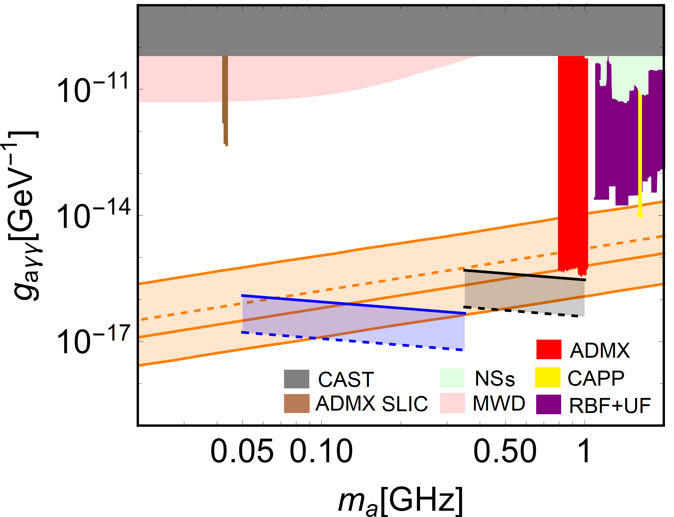
Figure 6: Projected sensitivity for the axion-photon coupling constant associated with a NS-UMCH encounter. The blue (black) lines use SKA1-low array (SKA-mid array) with $\displaystyle\text{SNR}_{\text{min}}=5$, efficiency $\displaystyle\eta_{s}=1$, and $\displaystyle\Delta B=\Delta\nu$. The rest of specifications are given in Table 1. For all cases, we take $\displaystyle M_{\text{UCMH}}=10^{2}\,M_{\text{PBH}}$ and $\displaystyle M_{\text{PBH}}=M_{\odot}$. The orange band is the QCD axion parameter of space, where we have marked the KSVZ (dashed line) and DFSZ (solid line) models. Current constraints on the axion-photon coupling constant are indicated with the remaining colored areas (see main text).

Array	SKA1-low	SKA-mid
P	0.5 s	0.5 s
$\displaystyle B_{0}$	$\displaystyle\mathcal{O}(10^{12})\,\text{G}$	$\displaystyle\mathcal{O}(10^{13})\,\text{G}$
$\displaystyle\theta$	$\displaystyle\pi/4$	$\displaystyle\pi/4$
$\displaystyle\theta_{m}$	$\displaystyle\pi/180$	$\displaystyle\pi/180$
d	300 pc	10 kpc
$\displaystyle\Delta t_{\text{obs}}$	100 hr	100 hr
$\displaystyle\Delta\nu$	30 kHz	100 kHz
r (solid)	$\displaystyle 10^{-5}\,R_{\text{UCMH}}$	$\displaystyle 10^{-5}\,R_{\text{UCMH}}$
r (dashed)	$\displaystyle 10^{-6}\,R_{\text{UCMH}}$	$\displaystyle 10^{-6}\,R_{\text{UCMH}}$

Table 1: Parameters used to calculate the projected sensitivity for the axion-photon coupling constant in Fig. 6 (blue and black dashed and solid lines).

Galactic pulsar surveys and simulations show that NSs spin period and magnetic field at poles obey both log-normal distributions, with a mean and dispersion given by $\displaystyle\text{log}_{10}(P/ms)=2.7$, $\displaystyle\sigma_{P}=-0.34$, Lorimer et al. (2006) and $\displaystyle\text{log}_{10}(B_{0}/G)=12.65$, $\displaystyle\sigma_{B_{0}}=0.55$, Faucher-Giguere and Kaspi (2006); Bates et al. (2014), respectively. Based on that, we consider NS-UCMH encounters involving typical galactic NSs with spin periods and magnetic fields around mean values. For a small misalignment angle in Eq. (81), such mean values lead to a broadened signal $\displaystyle\Delta\nu\sim(10-100)\,\text{kHz}$. We fix the signal bandwidth received by SKA1-low and SKA-mid radio telescope to be $\displaystyle 30\,\text{kHz}$ and $\displaystyle 100\,\text{kHz}$, respectively. As we explain later, for a given axion mass and NS properties, we choose the NS magnetic field at poles which is consistent with the predefined signal bandwidth.

Fig. 6 shows the projected sensitivity of the axion-photon coupling constant based on a NS-UCMH encounter by using the SKA1-low (blue lines) and SKA-mid (black lines) array. In all cases, we have taken $\displaystyle M_{\text{UCMH}}=10^{2}\,M_{\text{PBH}}$ with $\displaystyle M_{\text{PBH}}=M_{\odot}$, $\displaystyle M_{\text{NS}}=M_{\odot}$, and $\displaystyle R_{\text{NS}}=10\,\text{km}$. The NS properties and other parameters are given in detail in Table 1. While the orange band indicates the parameter space for the QCD axion, the other colored regions correspond to the different constraints over the axion-photon coupling constant O’Hare (2020) coming from CAST Andriamonje et al. (2007); Anastassopoulos et al. (2017) (gray), ADMX Bartram et al. (2021) (red), ADMX SLIC Crisosto et al. (2020) (brown), CAPP Lee et al. (2020) (yellow), RBF+UF DePanfilis et al. (1987); Hagmann et al. (1990) (purple), Neutron Stars Foster et al. (2020); Darling (2020a, b) (green), and MWD Dessert et al. (2022) (pink). The spectral density is estimated by using Eq. (78), where the axion density at the conversion radius is calculated from Eq. (79). For a given axion mass, misalignment angle, and spin period, we set the NS magnetic field at poles by requiring $\displaystyle\Delta\nu(B_{0})=\Delta B$, assuming that the optimized telescope bandwidth matches the signal bandwidth in Eq. (81). We see that for $\displaystyle r\sim(10^{-6}-10^{-5})\,\text{pc}$ and an observation time $\displaystyle\Delta t_{\text{obs}}=100\,\text{hr}$, the SKA telescope has the enough sensitivity to detect the QCD axion (orange band) from a source located at $\displaystyle\sim(0.1-10)\,\text{kpc}$.

Here we have considered typical parameter values for neutron stars in the Galaxy. However, the effect of their values on the QCD axion detection can readily be extracted by using Eqs. (78) and (81). In our estimation, for fixed observation angle and $\displaystyle\Delta B=\Delta\nu$, the minimun axion-photon coupling to be detectable for a given telescope array reads as

$$g_{a\gamma\gamma,\text{min}}\propto B_{0}^{-1/3}P^{-11/12}R_{\text{NS}}^{-1}M_{\text{NS}}^{-1/4}.$$ (84)

Generally speaking, we see that the larger the magnetic field or the longer the NS spin period, the better is the sensitivity. From Fig. 6, for example, we see that even neutron stars holding low magnetic fields as $\displaystyle B_{0}\sim 10^{10}\,\text{G}$ or short spin periods as $\displaystyle P\sim 0.1\,\text{s}$ should still lead to a detectable signal during a close encounter with an UCMH.

From the perspective of axion searches, the analyzed range for axion masses complements the current parameter space associated with the axion-photon coupling constant. In addition, our proposed scenario can be also studied in the context of multi-messenger astronomy by considering the situation where the NS undergoes an inspiral motion to the central PBH leading to the associated gravitational wave emission. Such a situation was analyzed by Edwards et al. (2020) in the context of intermediate black holes $\displaystyle(10^{3}-10^{5}\,)M_{\odot}$ having axion DM spikes around them. We leave this fascinating research avenue for a future work.

VIII Conclusion

In this work, we considered the axion DM scenario with the decay constant range $\displaystyle F_{a}\in[10^{12}{\rm GeV},10^{16}{\rm GeV}]$. Motivated by the story of axion embedded in either of supersymmetric models or string theory, we assumed a heavy scalar field $\displaystyle\sigma$ (saxion or moduli field) and studied the relic abundance of the axion DM during the EMD era in Sec. II and III. The presence of $\displaystyle\sigma$ was shown to lead to the EMD era and its decay prior to BBN era causes the late time entropy production. Thanks to the later, even for $\displaystyle\theta_{\rm i}=\mathcal{O}(1)$, the axion DM relic abundance was shown to be consistent with that of the current DM, i.e. $\displaystyle\Omega_{\rm DM}h^{2}\simeq 0.12$.

Keeping in mind the presence of the EMD era as the advantageous environment for formation of PBH, we considered an enhanced power spectrum of the primordial curvature perturbation at $\displaystyle k\gtrsim 10^{4}{\rm Mpc}^{-1}$. In Sec. IV, we showed how the assumed enhancement consistent with the constraint on $\displaystyle P_{\zeta}(k)$ could result in the formation of PBH with $\displaystyle f_{\rm PBH}=\mathcal{O}(10^{-3})$ for $\displaystyle M_{\rm PBH}\lesssim 10^{-6}M_{\odot}$ (case I) and $\displaystyle M_{\rm PBH}=\mathcal{O}(1)M_{\odot}$. PBHs so formed are expected to develop to UCMH with $\displaystyle M_{\rm UCMH}\simeq 10^{2}M_{\rm PBH}$ and $\displaystyle f_{\rm UCMH}\simeq 10^{2}f_{\rm PBH}$ as was discussed in Sec. V.

In Sec. VI and VII, we discussed how the UCMH can be of help in searching for the large decay constant axion DM. Firstly for the case I, UCMH can go through tidal disruption on high-speed encounters with stars. We computed the critical impact parameter $\displaystyle b_{c}$ numerically based on which we estimated the total probability for UCMH disruption. We found that for $\displaystyle M_{\rm PBH}\lesssim 10^{-6}M_{\odot}$, all UCMHs go through disruption. The disruption gives rise to the tidal stream with $\displaystyle\rho_{\text{st}}$ larger than the current local DM density, which could potentially improve the experimental sensitivity of ABRACADABRA Kahn et al. (2016) for $\displaystyle g_{a\gamma\gamma}$ during the time of the encounter between the tidal stream and the earth. Particularly for $\displaystyle M_{\rm PBH}$ as small as $\displaystyle\mathcal{O}(10^{-15})M_{\odot}$, the Earth can encounter the tidal stream of axion DM with the enhanced $\displaystyle\rho_{\text{st}}\gtrsim 10\,\rho_{\text{local}}$ for $\displaystyle M_{\text{PBH}}\lesssim 10^{-14}M_{\odot}$ once every (1-10) years (see Fig. 5).

For the case II, we attended to the possibility of transient radio signal generation when solar mass UCMHs encounter NSs. At the conversion radius $\displaystyle r_{c}$, the axion halo is expected to be converted into photons via the inverse Primakoff effect provided $\displaystyle m_{a}$ coincides with the plasma frequency. By considering (1) the Doppler broadening caused by temporal dependence from the co-rotation of the plasma with the NS, (2) the Liouville’s theorem for the axion density at the NS conversion radius, (3) typical NSs in the galaxy, and (4) an observation time of $\displaystyle 100\,\text{hr}$, we showed that the SKA1-low and SKA-mid telescope have the enough sensitivity to probe the parameter space $\displaystyle(m_{a},g_{a\gamma\gamma})$ as shown in Fig. 6.

In sum, we considered the non-standard cosmology with the EMD era as a way to save the axion DM scenario with $\displaystyle F_{a}\in[10^{12}{\rm GeV},10^{16}{\rm GeV}]$ from the dangerous overclosure of the universe. With the assumption for the enhanced $\displaystyle P_{\zeta}(k)$ on small scales, significant amount of PBHs can form during the EMD era, resulting in formation of UCMH during the late time matter domination era via secondary infall accretion. We point out that tidal streams and transient radio signals generated on UCMH’s encountering stars and NSs respectively can be possibly very helpful in searching for the large decay constant axion DM. Although not probed in this work, the induced gravitational wave due to the enhanced $\displaystyle P_{\zeta}(k)$ on small scales can be an interesting complementary experimental way to test our scenario Inomata et al. (2017).

Appendix A Hubble Expansion Rate at $\displaystyle t_{*}$

Define $\displaystyle t_{*}$ ($\displaystyle R_{*}$) to be the time (the scale factor) at which the EMD era gets started. Assume that the heavy particle $\displaystyle\sigma$ starts oscillation at the time of rh1. Then from the equality $\displaystyle\rho_{\sigma}(R_{*})\simeq\rho_{\rm rad}(R_{*})$, we obtain

$$\frac{1}{2}m_{\sigma}^{2}\sigma_{0}^{2}\left(\frac{R_{\rm rh1}}{R_{*}}\right)^{3}\simeq g_{*}(T_{\rm rh1})\frac{\pi^{2}}{30}T_{\rm rh1}^{4}\left(\frac{R_{\rm rh1}}{R_{*}}\right)^{4}\,,$$ (85)

where $\displaystyle\sigma_{0}$ is the initial field displacement from the origin in the field space, $\displaystyle m_{\sigma}$ is the mass of $\displaystyle\sigma$ and $\displaystyle T_{\rm rh1}$ is the reheating temperature defined via the inflaton perturbative decay rate $\displaystyle T_{\rm rh1}\simeq\sqrt{\Gamma_{\rm inflaton}M_{P}}$.

The ratio $\displaystyle R_{\rm rh1}/R_{*}$ being inferred from Eq. (85), we can $\displaystyle\rho_{\sigma}(R_{*})$

$$\rho_{\sigma}(R_{*})=\left(\frac{15^{3}}{2\pi^{6}g_{*}(T_{\rm rh1})^{3}}\right)\frac{m_{\sigma}^{8}\sigma_{0}^{8}}{T_{\rm rh1}^{12}}\,.$$ (86)

which in turn gives

$$H(R_{*})=\sqrt{\frac{15^{3}}{6\pi^{6}g_{*}(T_{\rm rh1})^{3}}}\frac{m_{\sigma}^{4}\sigma_{0}^{4}}{M_{P}T_{\rm rh1}^{6}}\,.$$ (87)

Since we assumed that the moduli starts oscillation at rh1, we have

$$\displaystyle m_{\sigma}^{2} \displaystyle\simeq \displaystyle H(a_{\rm rh1})^{2}=\frac{g_{*}(T_{\rm rh1})\frac{\pi^{2}}{30}T_{\rm rh1}^{4}}{3M_{P}^{2}}$$ (88)

$$\displaystyle\rightarrow \displaystyle\quad T_{\rm rh1}^{6}=m_{\sigma}^{3}\left(\frac{g_{*}(T_{\rm rh1})\frac{\pi^{2}}{30}}{3M_{P}^{2}}\right)^{-3/2}\,.$$ (90)

Finally by plugging Eq. (90) in Eq. (87), we get

$$H(R_{*})\equiv H_{*}=0.765m_{\sigma}\left(\frac{\sigma_{0}}{M_{P}}\right)^{4}\,.$$ (91)

Appendix B PBH Mass Range ($\displaystyle M_{\rm max}$ and $\displaystyle M_{\rm min}$)

When the overdensity associated with the wavenumber $\displaystyle k=R_{k}H(R_{k})$ goes through the gravitational collapse to form a PBH, the PBH’s mass is given by

$$M=\gamma M_{H}=\gamma\frac{4\pi M_{P}^{2}}{H}\,.$$ (92)

where $\displaystyle M_{H}=(4\pi/3)H^{-3}\rho_{\rm tot}$ is the horizon mass and $\displaystyle\gamma=1$ if $\displaystyle k$ re-entered the horizon at a matter dominated era. By replacing $\displaystyle H$ with $\displaystyle k/R_{k}$ and writing $\displaystyle R_{k}$ in terms of $\displaystyle R_{\rm rh2}$ and $\displaystyle T_{\rm rh2}$ based on the entropy conservation, one can find that PBH mass is mapped to $\displaystyle k$ via

$$\displaystyle M \displaystyle= \displaystyle\gamma\frac{2\pi^{3}}{45}\left(\frac{T_{0}}{k}\right)^{3}\frac{g_{s*}(T_{0})}{g_{s*}(T_{\rm rh2})}g_{*}(T_{\rm rh2})T_{\rm rh2}$$

$$\displaystyle\simeq \displaystyle 2.42M_{\odot}\times\left(\frac{k}{10^{6}{\rm Mpc}^{-1}}\right)^{-3}\left(\frac{T_{\rm rh2}}{10{\rm MeV}}\right)\,.$$

On observing Eq. (LABEL:eq:MPBH), it is realized that the minimum PBH mass $\displaystyle M_{\rm min}$ is associated with $\displaystyle k_{\rm min}$ re-entering the horizon at $\displaystyle R_{*}$ while $\displaystyle M_{\rm max}$ is so with $\displaystyle k_{\rm max}$ of which corresponding fluctuation grows to 1 at $\displaystyle R_{\rm rh2}$.

When the Fourier modes of primordial fluctuations lying in $\displaystyle k_{\rm rh2}<k<k_{\rm min}$ re-entered the horizon, the universe was in the EMD era. Both of $\displaystyle k_{\rm min}$ and $\displaystyle k_{\rm max}$ can be expressed in terms of $\displaystyle k_{\rm rh2}$. Aiming to calculate $\displaystyle k_{\rm min}$ and $\displaystyle k_{\rm max}$, we first compute $\displaystyle k_{\rm rh2}=R_{\rm rh2}H_{\rm rh2}$. From the entropy conservation, we have

$$\displaystyle R_{\rm rh2} \displaystyle= \displaystyle R_{\rm eq}\frac{g_{s*}(R_{\rm eq})^{\frac{1}{3}}T_{\rm eq}}{g_{s*}(R_{\rm rh2})^{\frac{1}{3}}T_{\rm rh2}}$$ (96)

$$\displaystyle\simeq \displaystyle 1.58\times 10^{-11}\left(\frac{T_{\rm rh2}}{10{\rm MeV}}\right)^{-1}\,,$$ (98)

where $\displaystyle g_{s*}(R_{\rm eq})=3.94$ and $\displaystyle g_{s*}(R_{\rm rh2})=10.75$ were used. Along with $\displaystyle H_{\rm rh2}=\Gamma_{\sigma}$ from Eq. (6), Eq. (98) gives

$$\displaystyle k_{\rm rh2} \displaystyle\simeq \displaystyle 4.3\times 10^{5}{\rm Mpc}^{-1}\times\left(\frac{T_{\rm rh2}}{10{\rm MeV}}\right)^{-1}\left(\frac{m_{\sigma}}{100{\rm TeV}}\right)^{3}\,.$$

(99)

On the other hand, from $\displaystyle k_{\rm min}/k_{\rm rh2}=(R_{*}H_{*})/(R_{\rm rh2}H_{\rm rh2})=(R_{\rm rh2}/R_{*})^{1/2}$, we can write $\displaystyle k_{\rm min}$ as

$$\displaystyle k_{\rm min} \displaystyle= \displaystyle k_{\rm rh2}\times\left(\frac{R_{\rm rh2}}{R_{*}}\right)^{1/2}$$ (100)

$$\displaystyle= \displaystyle k_{\rm rh2}\times\left(\frac{H_{*}}{H_{\rm rh2}}\right)^{1/3}$$

$$\displaystyle= \displaystyle k_{\rm rh2}\times(0.765m_{\sigma})^{1/3}\left(\frac{\sigma_{0}}{M_{P}}\right)^{4/3}\Gamma_{\sigma}^{-1/3}\,,$$

where we used $\displaystyle R_{\rm rh2}/R_{*}=(t_{\rm rh2}/t_{*})^{2/3}=(H_{*}/H_{\rm rh2})^{2/3}$ for the second equality, and $\displaystyle H_{\rm rh2}\simeq\Gamma_{\sigma}$ and $\displaystyle H_{*}$ in Eq. (91) for the last equality. Therefore, plugging Eq. (99) in Eq. (LABEL:eq:kmin) yields

$$\displaystyle k_{\rm min} \displaystyle\simeq \displaystyle 3.274\times 10^{14}{\rm Mpc}^{-1}$$

$$\displaystyle\times \displaystyle\left(\frac{T_{\rm rh2}}{10{\rm MeV}}\right)^{-1}\left(\frac{\sigma_{0}}{M_{P}}\right)^{\frac{4}{3}}\left(\frac{m_{\sigma}}{100{\rm TeV}}\right)^{\frac{7}{3}}\,.$$

As for $\displaystyle k_{\rm max}$, given that the primordial fluctuation associated with the wavenumber $\displaystyle k_{\rm max}$ grows to 1 after the horizon re-entry at $\displaystyle R_{\rm rh2}$, we have $\displaystyle\sigma\times(R_{\rm rh2}/R_{\rm hc})=1$. Here $\displaystyle k_{\rm max}$ is assumed to re-enter the horizon at $\displaystyle R_{\rm hc}$. Because of $\displaystyle R_{\rm rh2}/R_{\rm hc}=(H_{\rm hc}/H_{\rm rh2})^{2/3}$, this in turn gives

$$H_{\rm hc}\simeq\sigma^{-3/2}H_{\rm rh2}\,.$$ (108)

Hence, now that $\displaystyle M\propto k^{-3}$ and $\displaystyle M\propto H^{-1}$, we obtain

$$k_{\rm max}=k_{\rm rh2}\sigma_{\rm max}^{-1/2}\,.$$ (109)

Note that $\displaystyle\sigma_{\rm max}$ can be obtained from $\displaystyle\sigma_{\rm max}^{2}\simeq(2/5)^{2}P_{\zeta}(k_{\rm max})$ and it reads Bhattacharya et al. (2021)

$$\displaystyle\log\sigma_{\rm max} \displaystyle= \displaystyle 2\log\left(\frac{k_{\rm rh2}}{k_{p}}\right)-8\sigma_{p}^{2}$$

$$\displaystyle+ \displaystyle 2\sqrt{16\sigma_{p}^{4}-8\sigma_{p}^{2}\log\left(\frac{k_{\rm rh2}}{k_{p}}\right)+2\sigma_{p}^{2}\log\left(\frac{4A_{p}}{25}\right)}\,.$$

Appendix C More accurate UCMH profile

Under the approximation that the DM velocity dispersion at UCMH formation $\displaystyle\sigma_{\text{DM}}$ is not affected by the UCMHs themselves, the mean tangential velocity of the infalling DM particle as a function of the radius ($\displaystyle r$) and the redshift ($\displaystyle z$) is

$$\displaystyle v_{\text{rot}}(r,z)=\frac{\sigma_{\text{DM}}(z)R_{\text{UCMH}}(z)}{r}\approx 1.4\times 10^{-4}\,\text{km/s}\,\times\,$$

$$\displaystyle\left(\frac{1+z}{1000}\right)^{-1/2}\left(\frac{M_{\text{UCMH}}(z)}{M_{\odot}}\right)^{0.28}\frac{R_{\text{UCMH}}(z)}{r}\,,$$ (113)

where we have used Eq. (19) in Ricotti et al. (2008) and $\displaystyle R_{\rm UCMH}(z)$ in Eq. (55).

The radial infall regime breaks down when the tangential velocity of a DM particle which is falling at radius $\displaystyle r$ from the central PBH overpasses the local Keplerian orbital velocity

$$v_{\text{kep}}(r)=\frac{\sqrt{G_{N}M_{\text{UCMH}}(z)}}{r^{1/8}R_{\text{UCMH}}^{3/8}(z)}\,.$$ (114)

Equating $\displaystyle v_{\text{rot}}(r_{c})=v_{\text{kep}}(r_{c})$ yields

$$r_{\text{c}}\approx 6\times 10^{-7}\text{pc}\left(\frac{1000}{z_{\sigma}+1}\right)^{2.415}\left(\frac{M_{\text{PBH}}}{M_{\odot}}\right)^{0.272}\,,$$ (115)

which is in close agreement with Li et al. (2012). Here $\displaystyle r_{c}$ is the radius of the non-radial infall core and $\displaystyle z_{\sigma}$ is the redshift at which the UCMH collapses Ricotti and Gould (2009). Typical conservative estimate obeys the parametrization Li et al. (2012)

$$\rho_{\text{UCMH}}=\rho_{\text{UCMH}}(r_{c})\left(1+\frac{r}{r_{c}}\right)^{-9/4}\,.$$ (116)

Appendix D Ergodic Distribution Function for UCMHs

Here we determine the ergodic distribution function (DF)  associated with the UCMH spherically symmetric radial profile. Knowing the DF will allow us to determine the axion velocity distribution with respect to the UCMH radius. The UCMH radial profile is simply written as $\displaystyle\rho_{\text{UCMH}}(r)=\rho_{R}(R_{\text{UCMH}}/r)^{\gamma}$, where $\displaystyle\rho_{R}\equiv\rho_{\text{UCMH}}(R_{\text{UCMH}})$ and $\displaystyle\gamma=9/4$, Eq. (56). The enclosed UCMH mass at radius $\displaystyle r$ reads

$$\displaystyle M_{\text{UCMH}}(r) \displaystyle\approx 4\pi\int_{0}^{r}r^{\prime 2}\rho_{\text{UCMH}}(r^{\prime})dr^{\prime}\,,$$ (117)

$$\displaystyle\approx\frac{16\pi\rho_{R}R_{\text{UCMH}}^{3}}{3}\left(\frac{r}{R_{\text{UCMH}}}\right)^{3/4}\,,$$ (118)

where the approximation symbol comes from the fact that we have extended the lower limit of the integral to zero and we have also neglected the formation of a core at very small radius Bringmann et al. (2012). We define the UCMH relative potential as $\displaystyle\Psi(r)=-\Phi(r)+\Phi_{0}$ where $\displaystyle\Psi\rightarrow\Phi_{0}=0$ as $\displaystyle r\rightarrow\infty$. Under the approximation $\displaystyle M_{\text{UCMH}}(r)+M_{\text{PBH}}\approx M_{\text{UCMH}}(r)$ for sufficiently large $\displaystyle r$, we have

$$\rho_{\text{UCMH}}(\Psi)=\left(\frac{3\Psi}{16\pi G_{N}\rho_{R}^{8/9}R_{\text{UCMH}}^{2}}\right)^{9}\,,$$ (119)

where we have used $\displaystyle\Psi(r)=G_{N}M_{\text{UCMH}}(r)/r$ . Noting that $\displaystyle(d\rho_{\text{UCMH}}/d\Psi)|_{\Psi=0}=0$ and defining the relative energy $\displaystyle\xi=\Psi-\frac{1}{2}v_{a}^{2}$, with $\displaystyle v_{a}$ as the axion velocity, the (simplified) Eddington’s inversion formula for the DF reads as

$$f(\xi)=\frac{1}{\sqrt{8}\pi^{2}}\left[\int_{0}^{\xi}\frac{d^{2}\rho_{\text{UCMH}}}{d\Psi^{2}}\frac{d\Psi}{\sqrt{\xi-\Psi}}\right]\,,$$ (120)

Plugging Eq. (119) into Eq. (120), we find

$$\displaystyle f(\xi) \displaystyle=\frac{18\sqrt{2}\rho_{\text{UCMH}}(\Psi)}{\Psi^{9}\pi^{2}}\int_{0}^{\xi}\frac{\Psi^{7}}{\sqrt{\xi-\Psi}}d\Psi\,,$$ (121)

$$\displaystyle=\frac{A}{G_{N}^{9}\rho_{R}^{8}R_{\text{UCMH}}^{18}}\xi^{15/2}\,,$$ (122)

where $\displaystyle A=(2998927360\sqrt{2}\pi^{11}/19683)^{-1}$. Then, the axion speed distribution at a radius $\displaystyle r$ is written as

$$\displaystyle f(v_{a}|r) \displaystyle=4\pi v_{a}^{2}\frac{f(\Psi(r)-\frac{1}{2}v_{a}^{2})}{\rho_{\text{UCMH}}(r)}\,,$$ (123)

$$\displaystyle=\frac{32768\sqrt{2}}{715\pi}\frac{v_{a}^{2}(\Psi(r)-\frac{1}{2}v_{a}^{2})^{15/2}}{\Psi^{9}(r)}\,,$$ (124)

with the normalization

$$\int_{0}^{\sqrt{2\Psi(r)}}f(v_{a}|r)dv_{a}=1\,.$$ (125)

The axion velocity at a given radius within the UCMH can be estimated by using the dispersion velocity $\displaystyle\sigma(r)$ from the distribution function $\displaystyle f(v_{a}|r)$ as

$$\sigma^{2}(r)=\int_{0}^{\sqrt{2\Psi(r)}}v_{a}^{2}f(v_{a}|r)dv_{a}=0.3\Psi(r)\,.$$ (126)

By using Eq. (56), it is easy to show that the UMCH radius which encloses k-times the mass of the central PBH is estimated to be $\displaystyle r=R_{\text{UCMH}}(kM_{\text{PBH}}/M_{\text{UCMH}})^{4/3}$. For $\displaystyle M_{\text{UCMH}}=10^{2}\,M_{\text{PBH}}$, we have $\displaystyle r=2\times 10^{-3}R_{\text{UCMH}}$ (see Sec. II in  Hertzberg et al. (2020b)). As a result, for small radius $\displaystyle r$ such that $\displaystyle r\lesssim 2\times 10^{-3}\,R_{\text{UCMH}}$, we can make the approximation $\displaystyle M_{\text{UCMH}}(r)+M_{\text{PBH}}\approx M_{\text{PBH}}$. We thus write the relative potential as $\displaystyle\Psi(r)\approx\Psi_{\text{PBH}}(r)=G_{N}M_{\text{PBH}}/r$ so that the density is re-expressed in terms of that potential as

$$\rho_{\text{UCMH}}(\Psi_{\text{PBH}})=\rho_{R}\left(\frac{R_{\text{UCMH}}}{G_{N}M_{\text{PBH}}}\right)^{9/4}\Psi_{\text{PBH}}^{9/4}\,.$$ (127)

Following the same procedure as before, the axion DM speed distribution at a radius $\displaystyle r$ reads as

$$\displaystyle f(\xi)=\frac{45\Gamma[5/4]\rho_{R}}{16(2\pi)^{3/2}\Gamma[7/4]}\left(\frac{R_{\text{UCMH}}}{G_{N}M_{\text{PBH}}}\right)^{9/4}\xi^{3/4}\,,$$ (128)

$$\displaystyle f(v_{a}|r)=\frac{45\Gamma[5/4]}{4\sqrt{8\pi}\Gamma[7/4]}\frac{v_{a}^{2}(\Psi_{\text{PBH}}(r)-\frac{1}{2}v_{a}^{2})^{3/4}}{\Psi_{\text{PBH}}(r)^{9/4}}\,.$$ (129)

where the same normalization applied in Eq. (125) holds.

References

- Raffelt (2008) G. G. Raffelt, Lect. Notes Phys. 741, 51 (2008), arXiv:hep-ph/0611350 .
- Agrawal et al. (2018) P. Agrawal, G. Marques-Tavares, and W. Xue, JHEP 03, 049 (2018), arXiv:1708.05008 [hep-ph] .
- Kitajima et al. (2018) N. Kitajima, T. Sekiguchi, and F. Takahashi, Phys. Lett. B 781, 684 (2018), arXiv:1711.06590 [hep-ph] .
- Dvali (1995) G. R. Dvali, (1995), arXiv:hep-ph/9505253 .
- Co et al. (2019) R. T. Co, E. Gonzalez, and K. Harigaya, JHEP 05, 162 (2019), arXiv:1812.11186 [hep-ph] .
- Buen-Abad and Fan (2019) M. A. Buen-Abad and J. Fan, JHEP 12, 161 (2019), arXiv:1911.05737 [hep-ph] .
- Bernal et al. (2021) N. Bernal, Y. F. Perez-Gonzalez, Y. Xu, and O. Zapata, Phys. Rev. D 104, 123536 (2021), arXiv:2110.04312 [hep-ph] .
- Bernal et al. (2022) N. Bernal, C. S. Fong, Y. F. Perez-Gonzalez, and J. Turner, (2022), arXiv:2203.08823 [hep-ph] .
- de Carlos et al. (1993) B. de Carlos, J. A. Casas, F. Quevedo, and E. Roulet, Phys. Lett. B 318, 447 (1993), arXiv:hep-ph/9308325 .
- Banks et al. (1994) T. Banks, D. B. Kaplan, and A. E. Nelson, Phys. Rev. D 49, 779 (1994), arXiv:hep-ph/9308292 .
- Conlon (2006) J. P. Conlon, JHEP 05, 078 (2006), arXiv:hep-th/0602233 .
- Svrcek and Witten (2006) P. Svrcek and E. Witten, JHEP 06, 051 (2006), arXiv:hep-th/0605206 .
- Choi and Jeong (2007) K. Choi and K. S. Jeong, JHEP 01, 103 (2007), arXiv:hep-th/0611279 .
- Acharya et al. (2014) B. S. Acharya, G. Kane, and E. Kuflik, Int. J. Mod. Phys. A 29, 1450073 (2014), arXiv:1006.3272 [hep-ph] .
- Steinhardt and Turner (1983) P. J. Steinhardt and M. S. Turner, Phys. Lett. B 129, 51 (1983).
- Kawasaki et al. (1996) M. Kawasaki, T. Moroi, and T. Yanagida, Phys. Lett. B 383, 313 (1996), arXiv:hep-ph/9510461 .
- Kawasaki et al. (2016a) M. Kawasaki, T. T. Yanagida, and N. Yokozaki, Phys. Lett. B 753, 389 (2016a), arXiv:1510.04171 [hep-ph] .
- Akrami et al. (2020) Y. Akrami et al. (Planck), Astron. Astrophys. 641, A10 (2020), arXiv:1807.06211 [astro-ph.CO] .
- Ade et al. (2021) P. A. R. Ade et al. (BICEP, Keck), Phys. Rev. Lett. 127, 151301 (2021), arXiv:2110.00483 [astro-ph.CO] .
- Preskill et al. (1983) J. Preskill, M. B. Wise, and F. Wilczek, Phys. Lett. B 120, 127 (1983).
- Dine and Fischler (1983) M. Dine and W. Fischler, Phys. Lett. B 120, 137 (1983).
- Abbott and Sikivie (1983) L. F. Abbott and P. Sikivie, Phys. Lett. B 120, 133 (1983).
- Fox et al. (2004) P. Fox, A. Pierce, and S. D. Thomas, (2004), arXiv:hep-th/0409059 .
- Cicoli et al. (2016) M. Cicoli, K. Dutta, A. Maharana, and F. Quevedo, JCAP 08, 006 (2016), arXiv:1604.08512 [hep-th] .
- Hertzberg et al. (2008) M. P. Hertzberg, M. Tegmark, and F. Wilczek, Phys. Rev. D 78, 083507 (2008).
- Nelson and Xiao (2018) A. E. Nelson and H. Xiao, Phys. Rev. D 98, 063516 (2018), arXiv:1807.07176 [astro-ph.CO] .
- Georg and Watson (2017) J. Georg and S. Watson, JHEP 09, 138 (2017), arXiv:1703.04825 [astro-ph.CO] .
- Hertzberg and Yamada (2018) M. P. Hertzberg and M. Yamada, Phys. Rev. D 97, 083509 (2018), arXiv:1712.09750 [astro-ph.CO] .
- Mishra and Sahni (2020) S. S. Mishra and V. Sahni, JCAP 04, 007 (2020), arXiv:1911.00057 [gr-qc] .
- Garcia-Bellido and Ruiz Morales (2017) J. Garcia-Bellido and E. Ruiz Morales, Phys. Dark Univ. 18, 47 (2017), arXiv:1702.03901 [astro-ph.CO] .
- Ballesteros and Taoso (2018) G. Ballesteros and M. Taoso, Phys. Rev. D 97, 023501 (2018), arXiv:1709.05565 [hep-ph] .
- Kawasaki et al. (2016b) M. Kawasaki, A. Kusenko, Y. Tada, and T. T. Yanagida, Phys. Rev. D 94, 083523 (2016b), arXiv:1606.07631 [astro-ph.CO] .
- Germani and Prokopec (2017) C. Germani and T. Prokopec, Phys. Dark Univ. 18, 6 (2017), arXiv:1706.04226 [astro-ph.CO] .
- Bhaumik and Jain (2020) N. Bhaumik and R. K. Jain, JCAP 01, 037 (2020), arXiv:1907.04125 [astro-ph.CO] .
- Ballesteros et al. (2020a) G. Ballesteros, J. Rey, M. Taoso, and A. Urbano, JCAP 07, 025 (2020a), arXiv:2001.08220 [astro-ph.CO] .
- Braglia et al. (2020) M. Braglia, D. K. Hazra, F. Finelli, G. F. Smoot, L. Sriramkumar, and A. A. Starobinsky, JCAP 08, 001 (2020), arXiv:2005.02895 [astro-ph.CO] .
- Fumagalli et al. (2020) J. Fumagalli, S. Renaux-Petel, J. W. Ronayne, and L. T. Witkowski, (2020), arXiv:2004.08369 [hep-th] .
- Linde et al. (2013) A. Linde, S. Mooij, and E. Pajer, Phys. Rev. D 87, 103506 (2013), arXiv:1212.1693 [hep-th] .
- Bugaev and Klimai (2014) E. Bugaev and P. Klimai, Phys. Rev. D 90, 103501 (2014), arXiv:1312.7435 [astro-ph.CO] .
- Domcke et al. (2017) V. Domcke, F. Muia, M. Pieroni, and L. T. Witkowski, JCAP 07, 048 (2017), arXiv:1704.03464 [astro-ph.CO] .
- Garcia-Bellido et al. (1996) J. Garcia-Bellido, A. D. Linde, and D. Wands, Phys. Rev. D 54, 6040 (1996), arXiv:astro-ph/9605094 .
- Lyth (2011) D. H. Lyth, (2011), arXiv:1107.1681 [astro-ph.CO] .
- Bugaev and Klimai (2012) E. Bugaev and P. Klimai, Phys. Rev. D 85, 103504 (2012), arXiv:1112.5601 [astro-ph.CO] .
- Clesse and García-Bellido (2015) S. Clesse and J. García-Bellido, Phys. Rev. D 92, 023524 (2015), arXiv:1501.07565 [astro-ph.CO] .
- Kawasaki and Tada (2016) M. Kawasaki and Y. Tada, JCAP 08, 041 (2016), arXiv:1512.03515 [astro-ph.CO] .
- Ballesteros et al. (2020b) G. Ballesteros, J. Rey, and F. Rompineve, JCAP 06, 014 (2020b), arXiv:1912.01638 [astro-ph.CO] .
- Gow et al. (2021) A. D. Gow, C. T. Byrnes, P. S. Cole, and S. Young, JCAP 02, 002 (2021), arXiv:2008.03289 [astro-ph.CO] .
- Bhattacharya et al. (2021) S. Bhattacharya, A. Das, and K. Dutta, JCAP 10, 071 (2021), arXiv:2101.02234 [astro-ph.CO] .
- Harada et al. (2016) T. Harada, C.-M. Yoo, K. Kohri, K.-i. Nakao, and S. Jhingan, Astrophys. J. 833, 61 (2016), arXiv:1609.01588 [astro-ph.CO] .
- Carr (1975) B. J. Carr, Astrophys. J. 201, 1 (1975).
- Harada et al. (2013) T. Harada, C.-M. Yoo, and K. Kohri, Phys. Rev. D 88, 084051 (2013), [Erratum: Phys.Rev.D 89, 029903 (2014)], arXiv:1309.4201 [astro-ph.CO] .
- Aghanim et al. (2020) N. Aghanim et al. (Planck), Astron. Astrophys. 641, A6 (2020), [Erratum: Astron.Astrophys. 652, C4 (2021)], arXiv:1807.06209 [astro-ph.CO] .
- Young (2019) S. Young, Int. J. Mod. Phys. D 29, 2030002 (2019), arXiv:1905.01230 [astro-ph.CO] .
- Harada et al. (2017) T. Harada, C.-M. Yoo, K. Kohri, and K.-I. Nakao, Phys. Rev. D 96, 083517 (2017), [Erratum: Phys.Rev.D 99, 069904 (2019)], arXiv:1707.03595 [gr-qc] .
- Allsman et al. (2001) R. A. Allsman et al. (Macho), Astrophys. J. Lett. 550, L169 (2001), arXiv:astro-ph/0011506 .
- Tisserand et al. (2007) P. Tisserand et al. (EROS-2), Astron. Astrophys. 469, 387 (2007), arXiv:astro-ph/0607207 .
- Griest et al. (2014) K. Griest, A. M. Cieplak, and M. J. Lehner, Astrophys. J. 786, 158 (2014), arXiv:1307.5798 [astro-ph.CO] .
- Oguri et al. (2018) M. Oguri, J. M. Diego, N. Kaiser, P. L. Kelly, and T. Broadhurst, Phys. Rev. D 97, 023518 (2018), arXiv:1710.00148 [astro-ph.CO] .
- Niikura et al. (2019) H. Niikura, M. Takada, S. Yokoyama, T. Sumi, and S. Masaki, Phys. Rev. D 99, 083503 (2019), arXiv:1901.07120 [astro-ph.CO] .
- Croon et al. (2020) D. Croon, D. McKeen, N. Raj, and Z. Wang, Phys. Rev. D 102, 083021 (2020), arXiv:2007.12697 [astro-ph.CO] .
- Bertschinger (1985) E. Bertschinger, APJS 58, 39 (1985).
- Mack et al. (2007) K. J. Mack, J. P. Ostriker, and M. Ricotti, Astrophys. J. 665, 1277 (2007), arXiv:astro-ph/0608642 .
- Berezinsky et al. (2013) V. S. Berezinsky, V. I. Dokuchaev, and Y. N. Eroshenko, JCAP 11, 059 (2013), arXiv:1308.6742 [astro-ph.CO] .
- Ricotti and Gould (2009) M. Ricotti and A. Gould, Astrophys. J. 707, 979 (2009), arXiv:0908.0735 [astro-ph.CO] .
- Bringmann et al. (2012) T. Bringmann, P. Scott, and Y. Akrami, Phys. Rev. D 85, 125027 (2012), arXiv:1110.2484 [astro-ph.CO] .
- Adamek et al. (2019) J. Adamek, C. T. Byrnes, M. Gosenca, and S. Hotchkiss, Phys. Rev. D 100, 023506 (2019), arXiv:1901.08528 [astro-ph.CO] .
- Li et al. (2012) F. Li, A. L. Erickcek, and N. M. Law, Phys. Rev. D 86, 043519 (2012), arXiv:1202.1284 [astro-ph.CO] .
- Hertzberg et al. (2021) M. P. Hertzberg, S. Nurmi, E. D. Schiappacasse, and T. T. Yanagida, Phys. Rev. D 103, 063025 (2021), arXiv:2011.05922 [hep-ph] .
- Boucenna et al. (2018) S. M. Boucenna, F. Kuhnel, T. Ohlsson, and L. Visinelli, JCAP 07, 003 (2018), arXiv:1712.06383 [hep-ph] .
- Tinyakov et al. (2016) P. Tinyakov, I. Tkachev, and K. Zioutas, JCAP 01, 035 (2016), arXiv:1512.02884 [astro-ph.CO] .
- Carr and Sakellariadou (1999) B. J. Carr and M. Sakellariadou, apj 516, 195 (1999).
- Hertzberg et al. (2020a) M. P. Hertzberg, E. D. Schiappacasse, and T. T. Yanagida, Phys. Lett. B 807, 135566 (2020a), arXiv:1910.10575 [astro-ph.CO] .
- Binney and Tremaine (2008) J. Binney and S. Tremaine, Galactic Dynamics: Second Edition (Princeton University Press, 2008).
- Spitzer (1958) J. Spitzer, Lyman, apj 127, 17 (1958).
- Schneider et al. (2010) A. Schneider, L. Krauss, and B. Moore, Phys. Rev. D 82, 063525 (2010), arXiv:1004.5432 [astro-ph.GA] .
- Kuijken and Gilmore (1989) K. Kuijken and G. Gilmore, MNRAS 239, 571 (1989).
- Green and Goodwin (2007) A. M. Green and S. P. Goodwin, Monthly Notices of the Royal Astronomical Society 375, 1111 (2007), https://academic.oup.com/mnras/article-pdf/375/3/1111/3943831/mnras0375-1111.pdf .
- Kroupa (2002) P. Kroupa, Science 295, 82 (2002), arXiv:astro-ph/0201098 .
- Angus and Zhao (2007) G. W. Angus and H. Zhao, Mon. Not. Roy. Astron. Soc. 375, 1146 (2007), arXiv:astro-ph/0608580 .
- Bovy and Tremaine (2012) J. Bovy and S. Tremaine, Astrophys. J. 756, 89 (2012), arXiv:1205.4033 [astro-ph.GA] .
- Kahn et al. (2016) Y. Kahn, B. R. Safdi, and J. Thaler, Phys. Rev. Lett. 117, 141801 (2016), arXiv:1602.01086 [hep-ph] .
- Brandt (2016) T. D. Brandt, Astrophys. J. Lett. 824, L31 (2016), arXiv:1605.03665 [astro-ph.GA] .
- Hook et al. (2018) A. Hook, Y. Kahn, B. R. Safdi, and Z. Sun, Phys. Rev. Lett. 121, 241102 (2018), arXiv:1804.03145 [hep-ph] .
- McMillan (2017) P. J. McMillan, MNRAS 465, 76 (2017), arXiv:1608.00971 [astro-ph.GA] .
- Nurmi et al. (2021) S. Nurmi, E. D. Schiappacasse, and T. T. Yanagida, JCAP 09, 004 (2021), arXiv:2102.05680 [hep-ph] .
- Goldreich and Julian (1969) P. Goldreich and W. H. Julian, Astrophys. J. 157, 869 (1969).
- Edwards et al. (2020) T. D. P. Edwards, M. Chianese, B. J. Kavanagh, S. M. Nissanke, and C. Weniger, Phys. Rev. Lett. 124, 161101 (2020), arXiv:1905.04686 [hep-ph] .
- Liouville (1838) J. Liouville, J. Math. Pure. Appl. 3, 342 (1838).
- BEN (2020) Advances in Space Research 65, 856 (2020), high-resolution space-borne radio astronomy.
- Rajan et al. (2016) R. T. Rajan, A.-J. Boonstra, M. Bentum, M. Klein-Wolt, F. Belien, M. Arts, N. Saks, and A.-J. van der Veen, Experimental Astronomy 41, 271 (2016), arXiv:1505.04711 [astro-ph.IM] .
- Battye et al. (2021) R. A. Battye, B. Garbrecht, J. I. McDonald, and S. Srinivasan, JHEP 09, 105 (2021), arXiv:2104.08290 [hep-ph] .
- Battye et al. (2020) R. A. Battye, B. Garbrecht, J. I. McDonald, F. Pace, and S. Srinivasan, Phys. Rev. D 102, 023504 (2020), arXiv:1910.11907 [astro-ph.CO] .
- (93) “SKA1 SYSTEM BASELINE DESIGN,” https://www.skatelescope.org/wp-content/uploads/2012/07/SKA-TEL-SKO-DD-001-1_BaselineDesign1.pdf.
- Lorimer et al. (2006) D. R. Lorimer et al., Mon. Not. Roy. Astron. Soc. 372, 777 (2006), arXiv:astro-ph/0607640 .
- Faucher-Giguere and Kaspi (2006) C.-A. Faucher-Giguere and V. M. Kaspi, Astrophys. J. 643, 332 (2006), arXiv:astro-ph/0512585 .
- Bates et al. (2014) S. Bates, D. Lorimer, A. Rane, and J. Swiggum, Mon. Not. Roy. Astron. Soc. 439, 2893 (2014), arXiv:1311.3427 [astro-ph.IM] .
- O’Hare (2020) C. O’Hare, “cajohare/axionlimits: Axionlimits,” https://cajohare.github.io/AxionLimits/ (2020).
- Andriamonje et al. (2007) S. Andriamonje et al. (CAST), JCAP 04, 010 (2007), arXiv:hep-ex/0702006 .
- Anastassopoulos et al. (2017) V. Anastassopoulos et al. (CAST), Nature Phys. 13, 584 (2017), arXiv:1705.02290 [hep-ex] .
- Bartram et al. (2021) C. Bartram et al. (ADMX), Phys. Rev. Lett. 127, 261803 (2021), arXiv:2110.06096 [hep-ex] .
- Crisosto et al. (2020) N. Crisosto, P. Sikivie, N. S. Sullivan, D. B. Tanner, J. Yang, and G. Rybka, Phys. Rev. Lett. 124, 241101 (2020), arXiv:1911.05772 [astro-ph.CO] .
- Lee et al. (2020) S. Lee, S. Ahn, J. Choi, B. R. Ko, and Y. K. Semertzidis, Phys. Rev. Lett. 124, 101802 (2020), arXiv:2001.05102 [hep-ex] .
- DePanfilis et al. (1987) S. DePanfilis, A. C. Melissinos, B. E. Moskowitz, J. T. Rogers, Y. K. Semertzidis, W. U. Wuensch, H. J. Halama, A. G. Prodell, W. B. Fowler, and F. A. Nezrick, Phys. Rev. Lett. 59, 839 (1987).
- Hagmann et al. (1990) C. Hagmann, P. Sikivie, N. S. Sullivan, and D. B. Tanner, Phys. Rev. D 42, 1297 (1990).
- Foster et al. (2020) J. W. Foster, Y. Kahn, O. Macias, Z. Sun, R. P. Eatough, V. I. Kondratiev, W. M. Peters, C. Weniger, and B. R. Safdi, Phys. Rev. Lett. 125, 171301 (2020), arXiv:2004.00011 [astro-ph.CO] .
- Darling (2020a) J. Darling, Phys. Rev. Lett. 125, 121103 (2020a), arXiv:2008.01877 [astro-ph.CO] .
- Darling (2020b) J. Darling, Astrophys. J. Lett. 900, L28 (2020b), arXiv:2008.11188 [astro-ph.CO] .
- Dessert et al. (2022) C. Dessert, D. Dunsky, and B. R. Safdi, (2022), arXiv:2203.04319 [hep-ph] .
- Inomata et al. (2017) K. Inomata, M. Kawasaki, K. Mukaida, Y. Tada, and T. T. Yanagida, Phys. Rev. D 96, 123527 (2017), arXiv:1709.07865 [astro-ph.CO] .
- Ricotti et al. (2008) M. Ricotti, J. P. Ostriker, and K. J. Mack, Astrophys. J. 680, 829 (2008), arXiv:0709.0524 [astro-ph] .
- Hertzberg et al. (2020b) M. P. Hertzberg, E. D. Schiappacasse, and T. T. Yanagida, Phys. Rev. D 102, 023013 (2020b), arXiv:2001.07476 [astro-ph.CO] .