The Extremal GDoF Gain of Optimal versus Binary Power Control in $K$ User Interference Networks Is $\Theta(\sqrt{K})$

Abstract

Using ideas from Generalized Degrees of Freedom (GDoF) analyses and extremal network theory, this work studies the extremal gain of optimal power control over binary (on/off) power control, especially in large interference networks, in search of new theoretical insights. Whereas numerical studies have already established that in most practical settings binary power control is close to optimal, the extremal analysis shows not only that there exist settings where the gain from optimal power control can be quite significant, but also bounds the extremal values of such gains from a GDoF perspective. As its main contribution, this work explicitly characterizes the extremal GDoF gain of optimal over binary power control as $\Theta\left(\sqrt{K}\right)$ for all $K$. In particular, the extremal gain is bounded between $\lfloor\sqrt{K}\rfloor$ and $2.5\sqrt{K}$ for every $K$. For $K=2,3,4,5,6$ users, the precise extremal gain is found to be $1,3/2,2,9/4$ and $41/16$, respectively. Networks shown to achieve the extremal gain may be interpreted as multi-tier heterogeneous networks. It is worthwhile to note that because of their focus on asymptotic analysis, the sharp characterizations of extremal gains are valuable primarily from a theoretical perspective, and not as contradictions to the conventional wisdom that binary power control is generally close to optimal in practical, non-asymptotic settings.

I Introduction

The design of communication systems involves many optimization problems. The inherent combinatorial complexity of these optimizations often makes direct analysis infeasible, and motivates complementary approaches from theoretical and practical perspectives. On one hand, useful practical insights may be obtained from extensive numerical simulations. On the other hand, theoretical understanding may be advanced through extremal analyses, focused on identifying key cornerstones, e.g., asymptotic limits that are theoretically insightful. For instance, information theory often relies on extremal analysis (e.g., bounding the performance of the best code among all codes) under asymptotic (unbounded code length, unbounded complexity) relaxations to obtain theoretically insightful answers (channel capacity) that are complemented by numerical simulations to yield efficient communication designs.

As the focus shifts from channels to networks, the combinatorial challenge is further compounded. Additional tools have emerged to facilitate extremal/asymptotic theoretical analysis of wireless networks. Among these tools are the high SNR perspective taken by Generalized Degrees of Freedom (GDoF) studies [1], and more recently the idea of extremal network theory introduced in [2], i.e., the study of the extremal network settings that maximize the gain of one coding scheme over another. Extremal network theory and practical simulations complement each other — the latter focuses on what is likely to happen in settings of current practical interest, while the former tries to understand what is the best/worst scenario possible. Extremal network theory is particularly valuable for large networks that are beyond the reach of numerical simulations. For example, [2] studies the extremal GDoF gain from joint coding (transmitter cooperation) over separate coding in a $K$ user interference network with finite precision channel state information at the transmitters (finite precision CSIT), and shows that in the parameter regimes known as TIN, CTIN and SLS, the extremal gain is $1.5$, $2-1/K$, and $\Theta(\log(K))$, respectively. Remarkably, [3] finds that if secrecy constraints are imposed, then there is no gain from transmitter cooperation in the SLS regime, but the extremal gain grows unbounded when the regime is relaxed to the STIN regime. Beyond the $K$ user interference channel, extremal GDoF analysis has been applied by Joudeh and Caire in [4] to downlink cellular networks, modeled as interfering broadcast channels, to characterize the gains of cooperation among base stations. Building on these advances, in this work we apply the GDoF and extremal network theory framework to an aspect that is essential to wireless network design – power control [5, 6, 7, 8, 9, 10]. In particular, we explore the extremal GDoF gain of optimal power control versus binary (on/off) power control in a (large) $K$ user interference network, where all interference is treated as (Gaussian) noise.

Power control in conjunction with treating interference as noise (TIN) is one of the most widely prevalent ideas in wireless networks with multiple interfering links, because of its relative simplicity and robustness compared with other sophisticated schemes, such as rate-splitting [11, 12], structured codes [13, 14], and interference alignment [15]. It has been widely adopted for interference management in wireless local area networks [16] and homo-/heterogeneous cellular networks [17], and remains one of the main tools for interference management in emerging applications such as device-to-device (D2D) communications [18], vehicle-to-everything (V2X) [19] networks, and space-air-ground integrated networks [20]. With power control and TIN, the rate $R_{k}$ achieved by User $k$, where $k\in\{1,2,\cdots,K\}$, is simply expressed as a function of the user’s signal to interference and noise power ratio SINR_k, as $R_{k}=\log(1+\text{SINR}_{k})$, which gives rise to the problem of rate-optimization through power control. This problem has been the subject of extensive research. In general, the rate and power optimization problem is non-convex and NP-hard [21, 22]. Lower complexity suboptimal algorithms have been developed based on fixed-point iteration [23], iterative water-filling [24, 25], game theory [26], geometric programming [27], weighted mean square error [28], fractional programming [29], and machine-learning approaches [30, 31, 32, 33, 34]. On the other hand, closed form characterizations of maximum sum-rate achievable with optimal power control remain rare, with analytical efforts mostly limited to small networks [35, 36], or symmetric settings [37].

As an alternative to optimal power control, binary power control is also of much interest due to its lower implementation complexity. Binary power control refers to the transmission scheme where each transmitter operates at one of two power levels: it is either switched off completely, or it transmits at full power. Optimal binary power control is essentially equivalent to a scheduling scheme, with the only choice corresponding to the selection of active users. The rate region achievable with binary power control (and time-sharing) is characterized in [38]. Rate optimization within this rate region is essentially an NP-hard non-convex integer programming problem [39]. Lower complexity scheduling algorithms are developed based on message-passing [40], SINR heuristics [41, 42], information-theoretic insights [43, 44], fractional programming [45], and machine learning approaches [46, 47, 48]. Binary power control is found to be optimal for sum-rate maximization in many cases, e.g., multiple access channels[49], $2$-user interference channels with single carrier [35, 36, 50] and multiple carriers [51], $K$-user one-sided symmetric Wyner-type interference channels [52], networks where the transmission rate is an artificial linear function of the received power [53], and networks where either a geometric-arithmetic mean or low-SINR approximation is applicable [36]. Remarkably, numerical simulations of common communication network topologies such as cellular networks and D2D networks [54, 55, 56, 57, 58] suggest that binary power control has performance comparable to optimal power control. However, there are no known theoretical bounds on the worst-case sub-optimality penalty of binary power control relative to optimal power control. The extremal analysis undertaken in this paper is aimed at finding such bounds.

Some of the most analytically tractable characterizations of approximate rate regions with power control and TIN have emerged out of high-SNR analysis in the GDoF framework [1]. The GDoF region of the $K$ user interference channel with power control and TIN is known to be a union of polyhedra determined by the channel strength parameters [59]. The region is in general not convex unless time-sharing is allowed [60]. Algorithms for joint rate assignment and power control under the GDoF framework are developed in [61, 62, 63], and GDoF analyses have also inspired practical spectrum sharing solutions such as ITLinQ [43] and ITLinQ+ [44]. Notably, under certain parameter regimes, power control and TIN are known to be information theoretically optimal in the GDoF sense [59, 60, 2]. Nevertheless, despite their relative simplicity, even the GDoF characterizations suffer from the curse of dimensionality as we study large networks. For a $K$ user interference channel, the GDoF region achievable by power control and TIN is a union of an exponential (in $K$) number of regions (corresponding to all subsets of active users), each characterized by an exponential number of so-called cycle bounds, which makes it challenging to extract fundamental insights about large networks from their GDoF regions. This is the challenge that motivates the extremal network theory perspective introduced in [2], which we use in this work to compare optimal power control with binary power control, especially for large networks. Specifically we explore the extremal gain, defined by the supremum of the ratio of the sum GDoF corresponding to optimal and binary power control, across all possible network topologies. Our main result is that the extremal gain of optimal over binary power control is $\Theta(\sqrt{K})$. We also explicitly identify a class of network topologies that allow this extremal gain asymptotically at high SNR. Remarkably, these topologies may be interpreted as multi-tier heterogeneous networks. Thus, the extremal analysis adds surprising theoretical insights to the picture presented by numerical simulations — whereas the numerical studies shows that binary power control is close to optimal for most commonly studied network topologies, the theoretical analysis reveals exceptional network topologies where binary power control can be significantly suboptimal, and presents a tight (orderwise) bound on this suboptimality penalty. Interestingly, for smaller interference networks, with $K=2,3,4,5,6$ users, we explicitly characterize the exact extremal GDoF gain of optimal over binary power control as $1,3/2,2,9/4,41/65$, respectively.

Notation: For a real number $b$, $(b)^{+}$ and $\{b\}^{+}$ denote $\max\{0,b\}$. For a set $A$, $|A|$ denotes its cardinality. The set $\mathbb{N}$ collects all positive integers. For a positive integer $N$, define $[N]=\{1,2,\cdots,N\}$. For two functions $f(x),g(x)$, $f(x)=\Theta(g(x))$ if $c_{1}\leq\liminf_{x\rightarrow\infty}\left|\frac{f(x)}{g(x)}\right|\leq\limsup_{x\rightarrow\infty}\left|\frac{f(x)}{g(x)}\right|\leq c_{2}$ for some constant $c_{1},c_{2}>0$.

II System Model

We consider a $K$-user Gaussian interference channel where each of the transmitters and receivers is equipped with a single antenna. The signal observed by Receiver $k$ in the $t$-th channel use is,

$$Y_{k}(t) =\sum_{i=1}^{K}|h_{ki}|e^{j\theta_{ki}}\tilde{X}_{i}(t)+Z_{k}(t), \forall t\in[T],k\in[K],$$ (1)

where $h_{ki}\triangleq|h_{ki}|e^{j\theta_{ki}}$ is the channel coefficient between Transmitter $i$ and Receiver $j$, $\tilde{X}_{i}(t)$ is the complex-valued symbol sent by Transmitter $i$, subject to power constraint $\mathbb{E}[|\tilde{X}_{i}(t)|^{2}]\leq P_{i}$, and $Z_{k}(t)\sim\mathcal{CN}(0,1)$ is the additive white Gaussian noise (AWGN) at Receiver $k$. We assume perfect channel state information at the receivers (CSIR), while the transmitters know at least the magnitudes of the channel coefficients.

Following the standard GDoF formulation [1, 59], we translate (1) into the following,

$$Y_{k}(t) =\sum_{i=1}^{K}\sqrt{P^{\alpha_{ki}}}X_{i}(t)+Z_{k}(t), \forall t\in[T],k\in[K].$$ (2)

Here $X_{i}(t)$ is the complex-valued symbol sent from Transmitter $i$, subject to unit power constraint, i.e., $\mathbb{E}[|{X}_{i}(t)|^{2}]\leq 1$. The parameter $\alpha_{ki}\triangleq(\log|h_{ki}|^{2}P_{i})^{+}\geq 0$ is the channel strength parameter for the link between Transmitter $i$ and Receiver $k$. Note that the phase terms $e^{j\theta_{ki}}$ are omitted in (2), as they are inconsequential to the scheme of power control and treating interference as noise [59] which is the focus of this work. For compact notation, let us collect all $\alpha_{ij}$ into $\boldsymbol{\alpha}$ defined as

$$\boldsymbol{\alpha} =[\alpha_{ij}]_{i\in[K],j\in[K]},$$ (3)

which we will refer to as the network topology.

Next we formalize the scheme of power control and TIN. Message $W_{i}\in\mathcal{W}_{i}$ originating at Transmitter $i$ is encoded into codeword $X_{i}(t)$, $t\in[T]$, with Gaussian codebooks of rate $R_{i}=\frac{1}{T}\log_{2}|\mathcal{W}_{i}|$ and power $\mathbb{E}[|X_{t}|^{2}]=P^{r_{i}}\leq 1$, where $r_{i}\leq 0$ are called the power allocation variables. Let us define the vector of power allocation variables as

$$\boldsymbol{r} \triangleq(r_{1},r_{2},\cdots,r_{K}).$$ (4)

At each Receiver $i$, $i\in[K]$, the desired message is decoded by treating interference as noise, so that the following rate is achieved.

$$R_{i}(\boldsymbol{\alpha},P,\boldsymbol{r})=\log_{2}\left(1+\frac{P^{\alpha_{ii}+r_{i}}}{1+\sum_{k\in[K]\setminus\{i\}}P^{\alpha_{ik}+r_{k}}}\right).$$ (5)

We define $d_{i}(\boldsymbol{\alpha},\boldsymbol{r})$ as the GDoF limit for the $i^{th}$ user, i.e.,

$$d_{i}(\boldsymbol{\alpha},\boldsymbol{r})\triangleq\lim_{P\rightarrow\infty}\frac{R_{i}(\boldsymbol{\alpha},P,\boldsymbol{r})}{\log_{2}P} =\left(\alpha_{ii}+r_{i}-\max_{k\in[K]\setminus\{i\}}\{\alpha_{ik}+r_{k}\}^{+}\right)^{+},$$ (6)

where the second equality comes from [59, Eq. (7)]. The sum rate and sum GDoF achieved by power control and treating interference as noise are defined accordingly as,

$${R}_{\Sigma}(\boldsymbol{\alpha},P,\boldsymbol{r}) =\sum_{k=1}^{K}R_{i}(\boldsymbol{\alpha},P,\boldsymbol{r}),$$ (7)

$${D}_{\Sigma}(\boldsymbol{\alpha},\boldsymbol{r}) =\sum_{k=1}^{K}d_{i}(\boldsymbol{\alpha},\boldsymbol{r}).$$ (8)

II-A Optimal and Binary Power Control

The main goal of this work is to compare Optimal Power Control (OPC) against Binary Power Control (BPC). Let us define these two power control schemes under the GDoF framework. With OPC, the power exponents $r_{k}$ are allowed to take an arbitrary non-positive value, i.e., $r_{k}\leq 0$, for all $k\in[K]$. On the other hand, Binary Power Control (BPC) allows each $r_{i}$ to take only binary values, $-\infty$ and $0$. These two values correspond to the two operating states of a transmitter: the former is equivalent to switching it off, while the latter amounts to transmitting at full power. The sum rate with OPC and BPC are respectively defined as

$$R_{\Sigma,o}(\boldsymbol{\alpha},P) =\max_{\boldsymbol{r}\in\Omega^{K}}R_{\Sigma}(\boldsymbol{\alpha},P,\boldsymbol{r}),$$ (9)

$$R_{\Sigma,b}(\boldsymbol{\alpha},P) =\max_{\boldsymbol{r}\in\Omega_{b}^{K}}R_{\Sigma}(\boldsymbol{\alpha},P,\boldsymbol{r}),$$ (10)

where $\Omega^{K}=\{\boldsymbol{r}|-\infty\leq r_{k}\leq 0,\forall k\in[K]\}$, and $\Omega_{b}^{K}=\{\boldsymbol{r}|r_{k}\in\{-\infty,0\},\forall k\in[K]\}$. The sum GDoF with OPC, $D_{\Sigma,o}$, and the one with BPC, $D_{\Sigma,b}$, are defined accordingly, i.e.,

$$D_{\Sigma,o}(\boldsymbol{\alpha}) =\max_{\boldsymbol{r}\in\Omega^{K}}D_{\Sigma}(\boldsymbol{\alpha},\boldsymbol{r}),$$ (11)

$$D_{\Sigma,b}(\boldsymbol{\alpha}) =\max_{\boldsymbol{r}\in\Omega_{b}^{K}}D_{\Sigma}(\boldsymbol{\alpha},\boldsymbol{r}).$$ (12)

III Results: Extremal GDoF Gain

The sum GDoF with OPC (11) and the one with BPC (12) are both functions of the network topology $\boldsymbol{\alpha}$. The sum-GDoF gain, defined by the ratio of the sum GDoF achieved with OPC and BPC, also varies with different topologies. By taking the supremum over all possible topologies, we define the extremal GDoF gain for the $K$ user interference networks as,

$$\mu_{K} =\sup_{\boldsymbol{\alpha}\in\mathcal{A}_{K}}\frac{D_{\Sigma,o}(\boldsymbol{\alpha})}{D_{\Sigma,b}(\boldsymbol{\alpha})},$$ (13)

where $\mathcal{A}_{K}=\{\boldsymbol{\alpha}:~{}\alpha_{ij}\geq 0,\forall i,j\in[K]\}$ denotes the set of all possible network topologies $\boldsymbol{\alpha}$ for a $K$-user interference network. In the following theorem we identify the exact value of the extremal GDoF gain for small networks with $6$ or fewer users.

Theorem 1.

For interference networks with $K=2,3,4,5,6$ users, the exact value of the extremal GDoF gain $\mu_{K}$ of optimal over binary power control is listed in the following table.

$K$	$2$	$3$	$4$	$5$	$6$
$\mu_{K}$	$1$	$3/2$	$2$	$9/4$	$41/16$

The proof of Theorem 1 appears in Section V.

1. Network topologies that achieve the extremal GDoF gains $\mu_{3}=3/2,\mu_{4}=2,\mu_{5}=9/4$ and $\mu_{6}=41/16$ for $K=3,4,5,6$ users, respectively, are illustrated in Figure 5. These are extremal networks, because according to Theorem 1 for each value of $K$, no other topology can achieve a higher GDoF gain from optimal power control over binary power control.

2. While conventional wisdom backed by extensive numerical simulations has already established that for most networks binary power control tends to be close to optimal, evidently even for relatively smaller number of users there exist networks (as shown in Figure 5) where optimal power control achieves significant (e.g., factor of $2$ for $K=4$ users) gains in throughput over binary power control.

3. Apparently, $\mu_{K}$ is increasing with $K$. However, the rate of increase does not behave in a monotonic fashion. As $K$ takes values $2,3,4,5,6$, the successive increases in $\mu_{K}$ are $50\%,33\%,12.5\%,13.89\%$, respectively. This observation shows the difficulty of guessing the exact general functional form of $\mu_{K}$ from the study of smaller networks.

   heightadjust = all, valign=t [][] [][8cm]

   Figure 1: $\mu_{3}=3/2$

   [][8cm]

   Figure 2: $\mu_{4}=2$

   [][8cm]

   Figure 3: $\mu_{5}=9/4$

   [][8cm]

   Figure 4: $\mu_{6}=41/16$

   Figure 5: $K$ user interference networks achieving extremal GDoF gain $\mu_{K}=3/2,2,9/4,41/16$, respectively, for (a) $K=3$, (b) $K=4$, (c) $K=5$, and (d) $K=6$ users.

The extremal sum-GDoF gain metric $\mu_{K}$ is grounded in asymptotic (high-SNR) analysis because of analytical tractability and the potential for sharp insights that are difficult to obtain directly in finite-SNR regimes, especially for large networks. Intuitively, because extremal gains are likely to manifest in high SNR regimes in any case, we expect that the extremal sum-GDoF gain should closely reflect the unconstrained extremal sum-rate gain across all SNR regimes, i.e., without the restriction of $P\rightarrow\infty$. The following corollary of Theorem 1 confirms this intuition for smaller networks. The proof of Corollary 1 is relegated to Section V-F.

Corollary 1.

Consider the extremal sum-rate gain, which is defined for $K$ user interference networks as follows,

$$\eta_{K}=\sup_{\boldsymbol{\alpha}\in\mathcal{A}_{K},P\geq 0}\frac{R_{\Sigma,o}(\boldsymbol{\alpha},P)}{R_{\Sigma,b}(\boldsymbol{\alpha},P)}.$$ (14)

The extremal sum-rate gain $\eta_{K}$ is equal to the extremal sum-GDoF gain $\mu_{K}$ for For $K=2,3,4$, i.e.,

$K$	$2$	$3$	$4$
$\eta_{K}$	$1$	$\frac{3}{2}$	$2$

Next we proceed to the main goal of this work, i.e., to understand the extremal GDoF gain for large interference networks. Since the general form of the $\mu_{K}$ function is not readily apparent from the studies of small networks, we must directly explore large interference networks. Our main result is stated in the following theorem.

Theorem 2.

For $K$-user interference channels, the extremal sum-GDoF gain of optimal over binary power control, $\mu_{K}$, satisfies $\mu_{K}=\Theta(\sqrt{K})$. Specifically,

$$1\leq\liminf_{K\rightarrow\infty}\frac{\mu_{K}}{\sqrt{K}}\leq\limsup_{K\rightarrow\infty}\frac{\mu_{K}}{\sqrt{K}}\leq 5/2.$$ (15)

The proof of Theorem 2 is provided in Section VI.

1. The proof of Theorem 2 reveals the bounds $\lfloor\sqrt{K}\rfloor\leq\mu_{K}\leq 2.5\sqrt{K}$ for all $K\in\mathbb{N}$. Notably, these bounds are not only valid for large $K$, rather they hold for all $K$. The bounds can be further tightened to within a factor of $1.5$ of each other when $K$ is a perfect square.

2. An extremal network for $K=m^{2}$ users is shown in Figure 6 and has a hierarchical structure, with $m$ groups, each of which is comprised of $m$ users. The strength ($\alpha_{ij}$ values) of the interfering links emanating from the $g^{th}$ group of users, $g\in[m]$, is equal to $g-1$, as experienced by users in groups $1,2,\cdots,g$, while users in groups $g+1,\cdots,m$ see no interference from users in group $g,g-1,\cdots,1$. The desired links of users in group $g$ all have strength $\alpha_{ii}=g$.

   Figure 6: An interference network with $K=m^{2}$ users, that achieves sum-GDoF gain of $m=\sqrt{K}$ from optimal over binary power control.

IV Key Lemmas

Define a subset of all possible topologies $\mathcal{A}_{K}$ as,

$$\mathcal{A}_{K}^{+} \triangleq\left\{\boldsymbol{\alpha}:~{}\left(\exists\boldsymbol{r}\in\Omega^{K}\text{ s.t. }D_{\Sigma,o}(\boldsymbol{\alpha})=\sum_{i=1}^{K}d_{i}(\boldsymbol{\alpha},\boldsymbol{r})\right)\Rightarrow\left(\min_{i\in[K]}d_{i}(\boldsymbol{\alpha},\boldsymbol{r})>0\right)\right\},$$ (16)

which collects the $K$ user network topologies whose sum GDoF under OPC, $D_{\Sigma,o}(\boldsymbol{\alpha})$ can be achieved only by GDoF tuples with non-zero components. For example, the topology $\boldsymbol{\alpha}=[\alpha_{11},\alpha_{12};\alpha_{21},\alpha_{22}]=[1,0.25;0.25,1]$ for $K=2$ users, lies in $\mathcal{A}_{2}^{+}$, because its sum-GDoF value with OPC, $D_{\Sigma,o}(\boldsymbol{\alpha})=1.5$ can be achieved only with GDoF tuples $(d_{1},d_{2})=(1,0.5)$ or $(0.5,1)$, or any tuple lying on the line segment connecting these two tuples. All of these tuples have non-zero components. On the other hand, the topology $\boldsymbol{\alpha}=[1,0.5;0.5,1]$ does not lie in $\mathcal{A}_{2}^{+}$, because its sum GDoF, $D_{\Sigma,o}(\boldsymbol{\alpha})=1$, can be achieved by the tuple $(d_{1},d_{2})=(1,0)$.

Before proceeding to the proof of Theorem 1 and Theorem 2, we first present some observations and a key lemma that we will need for the converse arguments. As our first observation, the extremal gain found within $\mathcal{A}_{K}^{+}$ is non-decreasing in $K$.

Lemma 1.

For $K\in\mathbb{N}$,

$$\sup_{\boldsymbol{\alpha}\in\mathcal{A}_{K}^{+}}\frac{D_{\Sigma,o}(\boldsymbol{\alpha})}{D_{\Sigma,b}(\boldsymbol{\alpha})}\leq\sup_{\boldsymbol{\alpha}^{\prime}\in\mathcal{A}_{K+1}^{+}}\frac{D_{\Sigma,o}(\boldsymbol{\alpha}^{\prime})}{D_{\Sigma,b}(\boldsymbol{\alpha}^{\prime})}.$$ (17)

Proof.

The proof is straightforward because for any $K$ user topology $\boldsymbol{\alpha}\in\mathcal{A}_{K}^{+}$, we can add a $(K+1)^{th}$ user who neither causes nor suffers interference from any of the original $K$ users $(\alpha_{i,K+1}=\alpha_{K+1,i}=0,\forall i\in[K])$, and has a desired channel strength $\alpha_{K+1,K+1}=\epsilon>0$, to obtain a $K+1$ user topology, $\boldsymbol{\alpha}^{\prime}\in\mathcal{A}_{K+1}^{+}$. Since this $(K+1)^{th}$ user must contribute $\epsilon>0$ to the sum-GDoF optimal solution with either OPC or BPC, $D_{\Sigma,o}(\boldsymbol{\alpha}^{\prime})=D_{\Sigma,o}(\boldsymbol{\alpha})+\epsilon$, and $D_{\Sigma,b}(\boldsymbol{\alpha}^{\prime})=D_{\Sigma,b}(\boldsymbol{\alpha})+\epsilon$. Since $\epsilon$ can be chosen to be arbitrarily small, the RHS of (17) cannot be smaller than the LHS. ∎

The next lemma bounds the extremal GDoF gain from above by two upper bounds in two complementary topology subsets.

Lemma 2.

For $K\geq 2$,

$$\mu_{K}\leq\max\left\{\mu_{K-1},\sup_{\boldsymbol{\alpha}\in\mathcal{A}_{K}^{+}}\frac{D_{\Sigma,o}(\boldsymbol{\alpha})}{D_{\Sigma,b}(\boldsymbol{\alpha})}\right\}.$$ (18)

Proof.

If $\mu_{K}=\sup_{\boldsymbol{\alpha}\in\mathcal{A}_{K}^{+}}\frac{D_{\Sigma,o}(\boldsymbol{\alpha})}{D_{\Sigma,b}(\boldsymbol{\alpha})}$ then (18) holds. So let us assume the alternative, i.e.,

$$\mu_{K}=\sup_{\boldsymbol{\alpha}\in\mathcal{A}_{K}\setminus\mathcal{A}_{K}^{+}}\frac{D_{\Sigma,o}(\boldsymbol{\alpha})}{D_{\Sigma,b}(\boldsymbol{\alpha})}.$$

Consider any $K$ user topology $\tilde{\boldsymbol{\alpha}}_{K}\in\mathcal{A}_{K}\setminus\mathcal{A}_{K}^{+}$. By definition, the sum-GDoF value $D_{\Sigma,o}(\tilde{\boldsymbol{\alpha}}_{K})$ must be achieved with $d_{i}(\tilde{\boldsymbol{\alpha}}_{K},\boldsymbol{r})=0$ for some $i\in[K]$. Removing this user $i$, we obtain a $K-1$ user topology $\tilde{\boldsymbol{\alpha}}_{K-1}$. Since User $i$ contributed nothing to the sum-GDoF under OPC, removing this user cannot hurt, i.e., $D_{\Sigma,o}(\tilde{\boldsymbol{\alpha}}_{K-1})=D_{\Sigma,o}(\tilde{\boldsymbol{\alpha}}_{K})$. On the other hand, removing this user cannot help increase the sum-GDoF with BPC, because switching off this user was already an option in the original $K$ user topology under BPC. Therefore, $D_{\Sigma,b}(\tilde{\boldsymbol{\alpha}}_{K-1})\leq D_{\Sigma,b}(\tilde{\boldsymbol{\alpha}}_{K})$, and we have,

$$\frac{D_{\Sigma,o}(\tilde{\boldsymbol{\alpha}}_{K})}{D_{\Sigma,b}(\tilde{\boldsymbol{\alpha}}_{K})}\leq\frac{D_{\Sigma,o}(\tilde{\boldsymbol{\alpha}}_{K-1})}{D_{\Sigma,b}(\tilde{\boldsymbol{\alpha}}_{K-1})}\leq\mu_{K-1}.$$ (19)

Since this holds for all topologies $\tilde{\boldsymbol{\alpha}}_{K}\in\mathcal{A}_{K}\setminus\mathcal{A}_{K}^{+}$, we have the bound $\mu_{K}\leq\mu_{K-1}$, which concludes the proof. ∎

Lemma 3.

For any topology $\boldsymbol{\alpha}$ and any power allocation vector $\boldsymbol{r}=(r_{1},r_{2},\cdots,r_{K})\in\Omega^{K}$, with $r_{\max}\triangleq\max_{k\in[K]}r_{k}$,

$$d_{k}(\boldsymbol{\alpha},\boldsymbol{r}) =d_{k}(\boldsymbol{\alpha},\boldsymbol{r}^{\prime}), \forall k\in[K],$$ (20)

where the new power allocation vector $\boldsymbol{r}^{\prime}=(r^{\prime}_{1},r^{\prime}_{2},\cdots,r^{\prime}_{K})\in\Omega^{K}$ and

$$r^{\prime}_{k} =r_{k}-r_{\max}, \forall k\in[K].$$ (21)

Proof.

The transmit power levels ($r_{k}$, $k\in[K]$) of all users are elevated (e.g., as illustrated in Figure 7) by the same amount ($-r_{\max}$), until at least one user hits its maximum transmit power level $(0)$. The elevated power allocation variables $r_{i}^{\prime}$ are still valid $(\boldsymbol{r}^{\prime}\in\Omega^{K})$ because their values are not more than $0$. This can be seen as $r_{i}^{\prime}=r_{i}-\max_{j\in[K]}r_{j}\leq r_{i}-r_{i}=0$. With the new power allocation variables $r_{i}^{\prime}$, every receiver sees the same upward shift (increase by $-r_{\max}$) in its desired signal as well as all the interfering signals. The difference of power levels between desired signals and interference is therefore unaffected. As a result, the GDoF achieved by TIN are unchanged, i.e., (20) holds. ∎

Figure 7: An illustration of Lemma 3. The power allocation $\boldsymbol{r}^{\prime}$ is obtained from $\boldsymbol{r}$ by raising the power levels at all inputs by $-r_{\max}=0.5$. Both allocations achieve the same GDoF tuple $(d_{1},d_{2},d_{3})=(2.5,1,2)$.

Although Lemma 2 gives an upper bound for the extremal GDoF gain, it remains to explicitly bound the sum-GDoF gain in a topology subset $\mathcal{A}_{K}^{+}$. The following lemma serves as a key building block for bounding such a gain.

Lemma 4.

Consider any network topology $\tilde{\boldsymbol{\alpha}}=[\tilde{\alpha}_{ij}]_{i\in[K],j\in[K]}\in\mathcal{A}_{K}^{+}$, and any power allocation vector $\tilde{\boldsymbol{r}}=(\tilde{r}_{1},\tilde{r}_{2},\cdots,\tilde{r}_{K})\in\Omega^{K}$ that achieves $D_{\Sigma,o}(\tilde{\boldsymbol{\alpha}})$, i.e.,

$$D_{\Sigma,o}(\tilde{\boldsymbol{\alpha}}) =\sum_{k=1}^{K}d_{k}(\tilde{\boldsymbol{\alpha}},\tilde{\boldsymbol{r}}).$$ (22)

For any $\mathcal{S}=\{\beta_{1},\beta_{2},\cdots,\beta_{L}\}\subseteq[K]$ satisfying $\tilde{r}_{\beta_{1}}\geq\tilde{r}_{\beta_{2}}\geq\cdots\geq\tilde{r}_{\beta_{L}}$, we have

$$D_{\Sigma,b}(\tilde{\boldsymbol{\alpha}}) \geq\sum_{i=1}^{L-1}\left(d_{\beta_{i}}(\tilde{\boldsymbol{\alpha}},\tilde{\boldsymbol{r}})+\tilde{r}_{\beta_{L}}-\tilde{r}_{\beta_{i}}\right)+\left(d_{\beta_{L}}(\tilde{\boldsymbol{\alpha}},\tilde{\boldsymbol{r}})+\tilde{r}_{\beta_{L-1}}-\tilde{r}_{\beta_{L}}\right), \text{if }L>1,$$ (23)

$$D_{\Sigma,b}(\tilde{\boldsymbol{\alpha}}) \geq d_{\beta_{1}}(\tilde{\boldsymbol{\alpha}},\tilde{\boldsymbol{r}})-\tilde{r}_{\beta_{1}}, \text{if }L=1.$$ (24)

Remark 1.

For brevity, we will refer to the bounds (23), (24) as $B_{[\beta_{1},\beta_{2},\cdots,\beta_{L}]}$.

Proof.

First we note that, since $\tilde{\boldsymbol{\alpha}}\in\mathcal{A}_{K}^{+}$, by (6)

$${d}_{i}(\tilde{\boldsymbol{\alpha}},\tilde{\boldsymbol{r}})=\tilde{\alpha}_{ii}+\tilde{r}_{i}-\max_{k\in[K],k\neq i}(\tilde{\alpha}_{ik}+\tilde{r}_{k})^{+}>0$$ (25)

for all $i\in[K]$. For any $\mathcal{S}\subseteq[K]$, define $\boldsymbol{r}(\mathcal{S})=(r_{1}(\mathcal{S}),r_{2}(\mathcal{S}),\cdots,r_{K}(\mathcal{S}))\in\Omega^{K}_{b}$ as the power allocation that sets $r_{i}(\mathcal{S})=0$ if $i\in\mathcal{S}$ and $r_{i}(\mathcal{S})=-\infty$ if $i\notin\mathcal{S}$. In other words, the power allocation $\boldsymbol{r}(\mathcal{S})$ amounts to switching on all transmitters in $\mathcal{S}$ at full power, and switching off all transmitters not in $\mathcal{S}$. We note that

$$D_{\Sigma,b}(\tilde{\boldsymbol{\alpha}})=\max_{\mathcal{S}\subseteq[K]}D_{\Sigma}(\tilde{\boldsymbol{\alpha}},\boldsymbol{r}(\mathcal{S}))\geq D_{\Sigma}(\tilde{\boldsymbol{\alpha}},\boldsymbol{r}(\mathcal{S}))$$ (26)

for all $\mathcal{S}\subseteq[K].$ If $L=1$, i.e., $\mathcal{S}=\{\beta_{1}\}\subseteq[K]$, then the bound (24) is obtained from (26) as follows:

$$D_{\Sigma,b}(\tilde{\boldsymbol{\alpha}}) \geq D_{\Sigma}(\tilde{\boldsymbol{\alpha}},\boldsymbol{r}(\mathcal{S}))=\tilde{\alpha}_{\beta_{1}\beta_{1}}$$ (27)

$$\geq\left(\tilde{\alpha}_{\beta_{1}\beta_{1}}+\tilde{r}_{\beta_{1}}-\max_{k\in[K],k\neq\beta_{1}}(\tilde{\alpha}_{\beta_{1}k}+\tilde{r}_{k})^{+}\right)-\tilde{r}_{\beta_{1}}$$ (28)

$$=d_{\beta_{1}}(\tilde{\boldsymbol{\alpha}},\tilde{\boldsymbol{r}})-\tilde{r}_{\beta_{1}}.$$ (29)

Next we consider $L>1$, and prove the bound (23). We will create a new topology $\boldsymbol{\alpha}^{\prime}$ based on the given topology $\tilde{\boldsymbol{\alpha}}$, such that the sum GDoF under OPC remains the same, i.e., $D_{\Sigma,o}(\tilde{\boldsymbol{\alpha}})=D_{\Sigma,o}(\boldsymbol{\alpha}^{\prime})$, while the sum GDoF under BPC cannot be better but may be possibly reduced, i.e., $D_{\Sigma,b}(\tilde{\boldsymbol{\alpha}})\geq D_{\Sigma,b}(\boldsymbol{\alpha}^{\prime})$. The main idea is that given a power allocation $\tilde{\boldsymbol{r}}$, since the GDoF achieved by each user are limited only by the strongest interference signal seen by its receiver, if the cross-channel strengths of the remaining interferers to that receiver are increased so that every interfering signal is as strong as the original strongest interference signal, this does not hurt the GDoF achieved under OPC, but it can potentially reduce the GDoF achieved with BPC.

For any given subset of users $\mathcal{S}=\{\beta_{1},\beta_{2},\cdots,\beta_{L}\}$ and the given topology $\tilde{\boldsymbol{\alpha}}$, we define the new topology $\boldsymbol{\alpha}^{\prime}=[\alpha_{ij}^{\prime}]_{i\in[K],j\in[K]}$, such that for all $i,j\in[K]$,

$$\alpha_{ij}^{\prime}\triangleq\begin{cases}\tilde{\alpha}_{ij},&\text{if }(i=j)\lor(i\notin\mathcal{S})\lor(j\notin\mathcal{S}),\\ \max_{k\in\mathcal{S},k\neq i}(\tilde{\alpha}_{ik}+\tilde{r}_{k})^{+}-\tilde{r}_{j},&\text{otherwise.}\end{cases}$$ (30)

Note that $\alpha_{ij}^{\prime}\geq\tilde{\alpha}_{ij}$, since for $i,j\in\mathcal{S}$ and $i\neq j$, we have $\alpha_{ij}^{\prime}\geq(\tilde{\alpha}_{ij}+\tilde{r}_{j})^{+}-\tilde{r}_{j}\geq\tilde{\alpha}_{ij}+\tilde{r}_{j}-\tilde{r}_{j}=\tilde{\alpha}_{ij}$. Also note that relative to $\tilde{\boldsymbol{\alpha}}$ the new topology $\boldsymbol{\alpha}^{\prime}$ differs in only those cross-links that both emerge and terminate at users in $\mathcal{S}$. For such cross links, their strengths are lifted up to the extent that, with the power allocations $\tilde{\boldsymbol{r}}$, their interference levels at each receiver reach the maximal interference level at that receiver due to all undesired transmitters in $\mathcal{S}$ in the original topology $\tilde{\boldsymbol{\alpha}}$. Figure 8 illustrates an example of how the new topology $\boldsymbol{\alpha}^{\prime}$ is created from $\tilde{\boldsymbol{\alpha}}$, where we assume $\tilde{r}_{1}\geq\tilde{r}_{2}\geq\cdots\geq\tilde{r}_{K}$, choose $\mathcal{S}=[K]$ and focus on Receiver 1. We firstly identify the maximal interference level in the original topology in Figure 8(a) as $\max_{k\in\mathcal{S},k\neq 1}(\tilde{\alpha}_{1k}+\tilde{r}_{k})^{+}=\tilde{\alpha}_{12}+\tilde{r}_{2}$. Then in the new topology, we define $\alpha_{11}^{\prime}=\tilde{\alpha}_{11}$, and $\alpha_{1j}^{\prime}=\tilde{\alpha}_{12}+\tilde{r}_{2}-\tilde{r}_{j}$ for $j=2,3,\cdots,K$. In the new topology $\boldsymbol{\alpha}^{\prime}$ with the power allocations $\tilde{\boldsymbol{r}}$, the interference caused at Receiver $1$ by all undesired transmitters is thus at the same level, as shown in Figure 8(b). In the new topology $\boldsymbol{\alpha}^{\prime}$, the sum GDoF $D_{\Sigma,o}(\boldsymbol{\alpha}^{\prime})\geq D_{\Sigma,o}(\tilde{\boldsymbol{\alpha}})$ because the GDoF achieved by the original power allocation $\tilde{\boldsymbol{r}}$ remain unchanged in the new topology. On the other hand, because increasing the cross-channel strengths cannot help a TIN scheme under OPC, this implies that $D_{\Sigma,o}(\boldsymbol{\alpha}^{\prime})=D_{\Sigma,o}(\tilde{\boldsymbol{\alpha}})$. For the same reason, i.e., because increasing cross-channel strengths cannot help a TIN scheme under BPC, we have $D_{\Sigma,b}(\tilde{\boldsymbol{\alpha}})\geq D_{\Sigma,b}(\boldsymbol{\alpha}^{\prime})$.

Next, in the new topology $\boldsymbol{\alpha}^{\prime}$ let us apply the binary power allocation vector $\boldsymbol{r}(\mathcal{S})$, i.e., switch on the transmitters in $\mathcal{S}$ at full power and keep the remaining transmitters switched off. Obviously, $D_{\Sigma,b}(\boldsymbol{\alpha}^{\prime})\geq D_{\Sigma}(\boldsymbol{\alpha}^{\prime},\boldsymbol{r}(\mathcal{S}))$.

Next let us show that for $i\in\mathcal{S}$, we can further bound $d_{i}(\boldsymbol{\alpha}^{\prime},\boldsymbol{r}(\mathcal{S}))$ from below as

$$d_{i}(\boldsymbol{\alpha}^{\prime},\boldsymbol{r}(\mathcal{S})) \geq{d}_{i}(\tilde{\boldsymbol{\alpha}},\tilde{\boldsymbol{r}})-\tilde{r}_{i}+\min_{j\in\mathcal{S},j\neq i}\tilde{r}_{j}.$$ (31)

This is because, by the definition of $d_{i}(\boldsymbol{\alpha}^{\prime},\boldsymbol{r}(\mathcal{S}))$, we have for $i\in\mathcal{S}$,

$$d_{i}(\boldsymbol{\alpha}^{\prime},\boldsymbol{r}(\mathcal{S})) =\left(\tilde{\alpha}_{ii}-\max_{j\in\mathcal{S},j\neq i}\alpha_{ij}^{\prime}\right)^{+}$$ (32)

$$\geq\tilde{\alpha}_{ii}-\max_{j\in\mathcal{S},j\neq i}\alpha_{ij}^{\prime}$$ (33)

$$=\tilde{\alpha}_{ii}-\max_{j\in\mathcal{S},j\neq i}\left\{\max_{k\in\mathcal{S},k\neq i}(\tilde{\alpha}_{ik}+\tilde{r}_{k})^{+}-\tilde{r}_{j}\right\}$$ (34)

$$=\tilde{\alpha}_{ii}-\max_{k\in\mathcal{S},k\neq i}(\tilde{\alpha}_{ik}+\tilde{r}_{k})^{+}+\min_{j\in\mathcal{S},j\neq i}\tilde{r}_{j}$$ (35)

$$=\left((\tilde{\alpha}_{ii}+\tilde{r}_{i})-\max_{k\in\mathcal{S},k\neq i}(\tilde{\alpha}_{ik}+\tilde{r}_{k})^{+}\right)-\tilde{r}_{i}+\min_{j\in\mathcal{S},j\neq i}\tilde{r}_{j}$$ (36)

$$\geq\left((\tilde{\alpha}_{ii}+\tilde{r}_{i})-\max_{k\in[K],k\neq i}(\tilde{\alpha}_{ik}+\tilde{r}_{k})^{+}\right)-\tilde{r}_{i}+\min_{j\in\mathcal{S},j\neq i}\tilde{r}_{j}$$ (37)

$$={d}_{i}(\tilde{\boldsymbol{\alpha}},\tilde{\boldsymbol{r}})-\tilde{r}_{i}+\min_{j\in\mathcal{S},j\neq i}\tilde{r}_{j}.$$ (38)

Equality (34) follows from the definition of $\alpha_{ij}^{\prime}$ in (30). In (34) we note that the inner maximum is a constant with respect to the outer one; thus we have (35). Step (37) holds because we expand the scope of values over which the first maximum is taken, from $\mathcal{S}$ to $[K]$. Finally, (38) follows due to (25).

Summing up (31) for all $i\in\mathcal{S}$ and applying the assumption $\tilde{r}_{\beta_{1}}\geq\tilde{r}_{\beta_{2}}\geq\cdots\geq\tilde{r}_{\beta_{L}}$, we obtain

$$D_{\Sigma}(\boldsymbol{\alpha}^{\prime},\boldsymbol{r}(\mathcal{S}))\geq\sum_{i=1}^{L-1}\left(\tilde{d}_{\beta_{i}}(\tilde{\boldsymbol{\alpha}},\tilde{\boldsymbol{r}})-\tilde{r}_{\beta_{i}}+\tilde{r}_{\beta_{L}}\right)+\left(\tilde{d}_{\beta_{L}}(\tilde{\boldsymbol{\alpha}},\tilde{\boldsymbol{r}})-\tilde{r}_{\beta_{L}}+\tilde{r}_{\beta_{L-1}}\right).$$ (39)

By putting (39) together with $D_{\Sigma,b}(\tilde{\boldsymbol{\alpha}})\geq D_{\Sigma,b}(\boldsymbol{\alpha}^{\prime})\geq D_{\Sigma}(\boldsymbol{\alpha}^{\prime},\boldsymbol{r}(\mathcal{S}))$, we arrive at the bound in (23). ∎

(a)

(b)

Figure 8: Creating a new network topology by raising the strength levels of the cross links in the original one. The blue bars are the desired signals, while the red bars are the interfering signals. The heights of the colored bars denote their power levels in dB scale. (a) The signals at Receiver 1 under optimal power control in the original network. (b) The signals with the same power allocation in the new network.

The next lemma is essential to this work as it bounds the sum-GDoF gains as a function of $K$.

Lemma 5.

Let $m\in\mathbb{N}$. When $K\geq m^{2}$, there exists a topology $\boldsymbol{\alpha}^{*}\in\mathcal{A}_{K}$ such that

$$\frac{D_{\Sigma,o}(\boldsymbol{\alpha}^{*})}{D_{\Sigma,b}(\boldsymbol{\alpha}^{*})} \geq m.$$ (40)

On the other hand, when $K=m^{2}$, we have

$$\sup_{\boldsymbol{\alpha}\in\mathcal{A}_{K}^{+}}\frac{D_{\Sigma,o}(\boldsymbol{\alpha})}{D_{\Sigma,b}(\boldsymbol{\alpha})} \leq\frac{3}{2}m-\frac{1}{2}.$$ (41)

Proof.

First we show the lower bound (40) with a topology $\boldsymbol{\alpha}^{*}\in\mathcal{A}_{m^{2}}$ depicted in Figure 6. We divide the $m^{2}$ users into $m$ groups, each of which consists of $m$ users and is denoted by $\mathcal{G}_{i}$, $i\in\{1,2,...,m\}$, i.e.,

$$\mathcal{G}_{i}=\left\{(i-1)m+1,(i-1)m+2,...,im\right\}.$$ (42)

In each group $\mathcal{G}_{i}$, all direct links have strength equal to $i$. For cross links, each transmitter in the group $\mathcal{G}_{i}$ connects to each receiver in $\mathcal{G}_{j}$ with strength $i-1$, where $j\leq i$ and $i,j\in\{1,2,...,m\}$. All the other cross links are disconnected, i.e., transmitters in the $i^{th}$ group do not interfere with receivers in groups $i+1,i+2,\cdots,m$. As an example, when $m=2$, we get the $4$-user interference channel in Figure 5(b), where $\mathcal{G}_{1}=\{1,2\}$ and $\mathcal{G}_{2}=\{3,4\}$.

For the topology $\boldsymbol{\alpha}^{*}$, each user achieves one GDoF when the power allocation vector $\boldsymbol{r}^{*}=\left(r_{1}^{*},r_{2}^{*},\cdots,r_{K}^{*}\right)$ is set as

$$r_{k}^{*} =1-j, \forall k\in\mathcal{G}_{j},j\in[m].$$ (43)

Thus the sum GDoF $D_{\Sigma}(\boldsymbol{\alpha}^{*},\boldsymbol{r}^{*})=m^{2}$, implying that $D_{\Sigma,o}(\boldsymbol{\alpha}^{*})\geq m^{2}$. Now consider binary power control, where we either activate a user by switching his transmitter on at full power, or deactivate the user by switching his transmitter off. In the topology $\boldsymbol{\alpha}^{*}$, activating any one of the transmitters in group $\mathcal{G}_{i}$ at full power overwhelms all the receivers in $\mathcal{G}_{j}$, for all $j<i$; i.e., all users in $\bigcup_{j\in[K],j<i}\mathcal{G}_{j}$ get zero GDoF whether or not they are activated. This means that only the users in the group with the largest index will survive. So it suffices to consider one single group at a time and decide how many users in that group may be activated to maximize the sum GDoF. Activating one user in group $i$ yields sum-GDoF value of $i$, and activating $k$ users, $1<k\leq m$, in group $i$ yields a sum-GDoF value of $k$. The optimal value is therefore $D_{\Sigma,b}(\boldsymbol{\alpha}^{*})=m$, which is achieved by activating all $m$ users in one single group only, or by activating any one user in group $\mathcal{G}_{m}$. Therefore, we establish the lower bound $\frac{D_{\Sigma,o}(\boldsymbol{\alpha}^{*})}{D_{\Sigma,b}(\boldsymbol{\alpha}^{*})}\geq m$ for $K=m^{2}$. For $K\geq m^{2}$, the same lower bound still holds, because we can achieve the same bound with a topology $\boldsymbol{\alpha}^{*}\in\mathcal{A}_{K}$, where we copy the one depicted in Figure 6 to the first $m^{2}$ users, and remove all links associated with the rest $K-m^{2}$ users. Here we conclude the proof of (40).

Next, we show the upper bound (41) for any $\tilde{\boldsymbol{\alpha}}\in\mathcal{A}_{K}^{+}$ when $K=m^{2}$. Let $\tilde{\boldsymbol{r}}$ be a power allocation vector associated with $\tilde{\boldsymbol{\alpha}}$ as in Lemma 4. A key non-trivial step of the proof is the idea of partitioning the sum-GDoF in a particular way and applying bounds obtained from Lemma 4 to each partition. In the following we first present the bounds, and then the explicit sum-GDoF partition. Without loss of generality, let us assume that

$$\tilde{r}_{1}\geq\tilde{r}_{2}\geq\cdots\geq\tilde{r}_{K},$$ (44)

which carries no loss of generality because it only amounts to a labeling of users in this order.

First consider the bounds $B_{[i,i+1,...i+m-1]}$. With the assumption (44),

$$B_{[i,i+1,...i+m-1]}\implies D_{\Sigma,b}(\tilde{\boldsymbol{\alpha}})\geq\sum_{j=i}^{i+m-1}d_{j}(\tilde{\boldsymbol{\alpha}},\tilde{\boldsymbol{r}})-\sum_{j=i}^{i+m-3}\tilde{r}_{j}+(m-2)\tilde{r}_{i+m-1},$$ (45)

where $i\in[m^{2}-m+1]$. Adding the bounds $\sum_{i=1}^{m^{2}-m+1}B_{[i,i+1,...i+m-1]}$ we obtain

$$(m^{2}-m+1)D_{\Sigma,b}(\tilde{\boldsymbol{\alpha}})$$

$$\geq\sum_{j=1}^{m-1}jd_{j}(\tilde{\boldsymbol{\alpha}},\tilde{\boldsymbol{r}})-\sum_{j=1}^{m-2}j\tilde{r}_{j}-(m-2)\tilde{r}_{m-1}+\sum_{j=m}^{m^{2}-m+1}md_{j}(\tilde{\boldsymbol{\alpha}},\tilde{\boldsymbol{r}})$$

$$\quad+\sum_{j=1}^{m-1}(m-j)d_{m^{2}-m+1+j}(\tilde{\boldsymbol{\alpha}},\tilde{\boldsymbol{r}})+\sum_{j=1}^{m-2}j\tilde{r}_{m^{2}-m+1+j}+(m-2)\tilde{r}_{m^{2}}.$$ (46)

Then we consider the bounds $B_{[1,2,...,i]}$, which are obtained from Lemma 4 and the assumption (44):

$$B_{[1]} \implies D_{\Sigma,b}(\tilde{\boldsymbol{\alpha}})\geq d_{1}(\tilde{\boldsymbol{\alpha}},\tilde{\boldsymbol{r}})-\tilde{r}_{1},$$ (47)

$$B_{[1,2,...,i]} \implies D_{\Sigma,b}(\tilde{\boldsymbol{\alpha}})\geq\sum_{j=1}^{i}d_{j}(\tilde{\boldsymbol{\alpha}},\tilde{\boldsymbol{r}})-\sum_{j=1}^{i-2}\tilde{r}_{j}+(i-2)\tilde{r}_{i},$$ (48)

where $i=2,3,\cdots,m-1$. Adding $B_{[1]}+\sum_{i=2}^{m-1}B_{[1,2,...,i]}$, we obtain,

$$(m-1)D_{\Sigma,b}(\tilde{\boldsymbol{\alpha}})$$

$$\geq\sum_{j=1}^{m-1}(m-j)d_{j}(\tilde{\boldsymbol{\alpha}},\tilde{\boldsymbol{r}})-\tilde{r}_{1}-\sum_{j=1}^{m-3}(m-2-j)\tilde{r}_{j}+\sum_{j=3}^{m-1}(j-2)\tilde{r}_{j}$$ (49)

$$\geq\sum_{j=1}^{m-1}(m-j)d_{j}(\tilde{\boldsymbol{\alpha}},\tilde{\boldsymbol{r}})+\sum_{j=3}^{m-1}(j-2)\tilde{r}_{j},$$ (50)

where (50) holds because $\tilde{r}_{j}\leq 0$ for $j\in[m^{2}]$.

Next we consider the bounds $B_{[i+m^{2}-m+1]}$ together with (44),

$$B_{[i+m^{2}-m+1]}\implies D_{\Sigma,b}(\tilde{\boldsymbol{\alpha}})\geq d_{i+m^{2}-m+1}(\tilde{\boldsymbol{\alpha}},\tilde{\boldsymbol{r}})-\tilde{r}_{i+m^{2}-m+1},$$ (51)

where $i=1,2,\cdots,m-1$. Adding $\sum_{i=1}^{m-1}iB_{[i+m^{2}-m+1]}$ we obtain,

$$\sum_{i=1}^{m-1}iD_{\Sigma,b}(\tilde{\boldsymbol{\alpha}})=\frac{1}{2}m(m-1)D_{\Sigma,b}(\tilde{\boldsymbol{\alpha}})$$

$$\geq\sum_{i=1}^{m-1}\Big{(}id_{i+m^{2}-m+1}(\tilde{\boldsymbol{\alpha}},\tilde{\boldsymbol{r}})-i\tilde{r}_{i+m^{2}-m+1}\Big{)}.$$ (52)

Finally, we sum up the bounds (46), (50) and (52) and obtain

$$m\left(\frac{3}{2}m-\frac{1}{2}\right)D_{\Sigma,b}(\tilde{\boldsymbol{\alpha}})$$

$$=\left[(m^{2}-m+1)+(m-1)+\frac{1}{2}m(m-1)\right]D_{\Sigma,b}(\tilde{\boldsymbol{\alpha}})$$ (53)

$$\geq mD_{\Sigma,o}(\tilde{\boldsymbol{\alpha}})-\tilde{r}_{1}-2\sum_{j=2}^{m-2}\tilde{r}_{j}-\tilde{r}_{m-1}-\tilde{r}_{m^{2}}$$ (54)

$$\geq mD_{\Sigma,o}(\tilde{\boldsymbol{\alpha}}),$$ (55)

where (55) holds because $\tilde{r_{i}}\leq 0$ for all $i\in[m^{2}]$. Since inequality (55) holds for all $\boldsymbol{\alpha}\in\mathcal{A}_{K}^{+}$ regardless of the assumption (44), we have

$$\sup_{\boldsymbol{\alpha}\in\mathcal{A}_{K}^{+}}\frac{D_{\Sigma,o}(\boldsymbol{\alpha})}{D_{\Sigma,b}(\boldsymbol{\alpha})}\leq\frac{3}{2}m-\frac{1}{2},$$ (56)

which concludes the proof of (41). ∎

V Proof of Theorem 1

V-A Case: $K=2$

It is known from [35, 36] already that binary power control is optimal for sum rate maximization in the $2$ user interference channel. This result applies to every SNR setting, and thus also to the GDoF framework, yielding $\mu_{2}=1$. However, in order to lay the foundation of the proof for subsequent cases, let us present an alternative proof based on Lemma 4. Since OPC cannot be worse than BPC, the lower bound is trivial in this case, i.e., $\mu_{2}\geq 1$. Now consider the converse. For any network topology $\tilde{\boldsymbol{\alpha}}\in\mathcal{A}_{2}^{+}$ and power allocation vector $\tilde{\boldsymbol{r}}$ as in Lemma 4, we apply the bound $B_{[1,2]}$,

$$B_{[1,2]} \implies D_{\Sigma,b}(\tilde{\boldsymbol{\alpha}})\geq(d_{1}(\tilde{\boldsymbol{\alpha}},\tilde{\boldsymbol{r}})-\tilde{r}_{1}+\tilde{r}_{2})+(d_{2}(\tilde{\boldsymbol{\alpha}},\tilde{\boldsymbol{r}})-\tilde{r}_{2}+\tilde{r}_{1})=D_{\Sigma,o}(\tilde{\boldsymbol{\alpha}}).$$ (57)

Therefore, we have $\sup_{\boldsymbol{\alpha}\in\mathcal{A}_{2}^{+}}\frac{D_{\Sigma,o}(\boldsymbol{\alpha})}{D_{\Sigma,b}(\boldsymbol{\alpha})}\leq 1$, and Lemma 2 yields the desired outer bound $\mu_{2}\leq\max\{\mu_{1},1\}=1$. $\hfill\square$

V-B Case: $K=3$

Let us start with the converse. For any network topology $\tilde{\boldsymbol{\alpha}}\in\mathcal{A}_{3}^{+}$, and the power allocation vector $\tilde{\boldsymbol{r}}$ as in Lemma 4, the bounds $B_{[1,2]},B_{[2,3]}$ and $B_{[1,3]}$ follow the same reasoning in (57) as follows:

$$B_{[1,2]} \implies D_{\Sigma,b}(\tilde{\boldsymbol{\alpha}})\geq d_{1}(\tilde{\boldsymbol{\alpha}},\tilde{\boldsymbol{r}})+d_{2}(\tilde{\boldsymbol{\alpha}},\tilde{\boldsymbol{r}}),$$ (58)

$$B_{[2,3]} \implies D_{\Sigma,b}(\tilde{\boldsymbol{\alpha}})\geq d_{2}(\tilde{\boldsymbol{\alpha}},\tilde{\boldsymbol{r}})+d_{3}(\tilde{\boldsymbol{\alpha}},\tilde{\boldsymbol{r}}),$$ (59)

$$B_{[1,3]} \implies D_{\Sigma,b}(\tilde{\boldsymbol{\alpha}})\geq d_{1}(\tilde{\boldsymbol{\alpha}},\tilde{\boldsymbol{r}})+d_{3}(\tilde{\boldsymbol{\alpha}},\tilde{\boldsymbol{r}}).$$ (60)

Summing up (58)–(60), we have $\sup_{\boldsymbol{\alpha}\in\mathcal{A}_{3}^{+}}\frac{D_{\Sigma,o}(\boldsymbol{\alpha})}{D_{\Sigma,b}(\boldsymbol{\alpha})}\leq 3/2$. By Lemma 2 we conclude the outer bound $\mu_{3}\leq\max\{\mu_{2},3/2\}=3/2.$

Next, for the lower bound on $\mu_{3}$, we consider the topology, say $\boldsymbol{\alpha}_{3}$, depicted in Figure 5(a). This topology has direct links set with strengths $\alpha_{11}=\alpha_{22}=1$ and $\alpha_{33}=2$. The (red) cross links are set with strength 1. With the power allocation $\boldsymbol{r}_{3}=(0,0,-1)$, we achieve the GDoF tuple $(1,1,1)$, hence $D_{\Sigma,o}(\boldsymbol{\alpha}_{3})\geq 3$. It is not difficult to exhaustively verify that with binary power control $D_{\Sigma,b}(\boldsymbol{\alpha}_{3})=2$. Therefore, we establish the lower bound $\mu_{3}\geq 3/2$. Since the lower bound matches the upper bound, we have $\mu_{3}=3/2$, which completes the proof for the case of $K=3$ users. $\hfill\square$

V-C Case: $K=4$

Start with the converse. For any network topology in $\tilde{\boldsymbol{\alpha}}\in\mathcal{A}_{4}^{+}$, and the power allocation vector $\tilde{\boldsymbol{r}}$ as in Lemma 4, we have the following bounds, similar to (57):

$$B_{[1,2]} \implies D_{\Sigma,b}(\tilde{\boldsymbol{\alpha}})\geq d_{1}(\tilde{\boldsymbol{\alpha}},\tilde{\boldsymbol{r}})+d_{2}(\tilde{\boldsymbol{\alpha}},\tilde{\boldsymbol{r}}),$$ (61)

$$B_{[3,4]} \implies D_{\Sigma,b}(\tilde{\boldsymbol{\alpha}})\geq d_{3}(\tilde{\boldsymbol{\alpha}},\tilde{\boldsymbol{r}})+d_{4}(\tilde{\boldsymbol{\alpha}},\tilde{\boldsymbol{r}}).$$ (62)

Adding (61)–(62) we obtain $\sup_{\boldsymbol{\alpha}\in\mathcal{A}_{4}^{+}}\frac{D_{\Sigma,o}(\boldsymbol{\alpha})}{D_{\Sigma,b}(\boldsymbol{\alpha})}\leq 2$. Then we apply Lemma 2 we get the desired upper bound $\mu_{4}\leq\max\{\mu_{3},2\}=2$.

For the lower bound, we consider the topology, say $\boldsymbol{\alpha}_{4}$, depicted in Figure 6(b), where the direct links have strengths $\alpha_{11}=\alpha_{22}=1$ and $\alpha_{33}=\alpha_{44}=2$, and the (red) cross links have strength 1. We achieve GDoF tuple $(1,1,1,1)$ with the power allocation $\boldsymbol{r}_{4}=(0,0,-1,-1)$, so $D_{\Sigma,o}(\boldsymbol{\alpha}_{4})\geq 4$. For binary power control, by considering all $2^{4}$ possible power allocation vectors, we find $D_{\Sigma,b}(\boldsymbol{\alpha}_{4})=2$. Therefore, we establish the lower bound $\mu_{4}\geq 2$. Since the lower bound matches the upper bound, we have $\mu_{4}=2$, which completes the proof for the case of $K=4$ users. $\hfill\square$

V-D Case: $K=5$

Again, let us start with the converse. Consider any network topology $\tilde{\boldsymbol{\alpha}}\in\mathcal{A}_{5}^{+}$, and any associated power allocation vector $\tilde{\boldsymbol{r}}$ as in Lemma 4. Without loss of generality, we further assume

$$0\geq\tilde{r}_{1}\geq\tilde{r}_{2}\geq\cdots\geq\tilde{r}_{5}.$$ (63)

The assumption that $\tilde{r}_{1}\geq\tilde{r}_{2}\geq\cdots\geq\tilde{r}_{5}$ incurs no loss of generality since it is equivalent to the labeling of users in this order. The assumption $\tilde{r}_{1}=0$, which means that User $1$ transmits at full power, is justified by Lemma 3. By Lemma 4 and the assumption (63), we have the following bounds.

$$B_{[5]} \implies D_{\Sigma,b}(\tilde{\boldsymbol{\alpha}})\geq d_{5}(\tilde{\boldsymbol{\alpha}},\tilde{\boldsymbol{r}})-\tilde{r}_{5},$$ (64)

$$B_{[1,2]} \implies D_{\Sigma,b}(\tilde{\boldsymbol{\alpha}})\geq d_{1}(\tilde{\boldsymbol{\alpha}},\tilde{\boldsymbol{r}})+d_{2}(\tilde{\boldsymbol{\alpha}},\tilde{\boldsymbol{r}}),$$ (65)

$$B_{[1,4]} \implies D_{\Sigma,b}(\tilde{\boldsymbol{\alpha}})\geq d_{1}(\tilde{\boldsymbol{\alpha}},\tilde{\boldsymbol{r}})+d_{3}(\tilde{\boldsymbol{\alpha}},\tilde{\boldsymbol{r}}),$$ (66)

$$B_{[2,4]} \implies D_{\Sigma,b}(\tilde{\boldsymbol{\alpha}})\geq d_{2}(\tilde{\boldsymbol{\alpha}},\tilde{\boldsymbol{r}})+d_{4}(\tilde{\boldsymbol{\alpha}},\tilde{\boldsymbol{r}}),$$ (67)

$$B_{[1,2,3]} \implies D_{\Sigma,b}(\tilde{\boldsymbol{\alpha}})\geq(d_{1}(\tilde{\boldsymbol{\alpha}},\tilde{\boldsymbol{r}})+\tilde{r}_{3})+(d_{2}(\tilde{\boldsymbol{\alpha}},\tilde{\boldsymbol{r}})-\tilde{r}_{2}+\tilde{r}_{3})+(d_{3}(\tilde{\boldsymbol{\alpha}},\tilde{\boldsymbol{r}})-\tilde{r}_{3}+\tilde{r}_{2}),$$ (68)

$$B_{[3,4,5]} \implies D_{\Sigma,b}(\tilde{\boldsymbol{\alpha}})\geq(d_{3}(\tilde{\boldsymbol{\alpha}},\tilde{\boldsymbol{r}})-\tilde{r}_{3}+\tilde{r}_{5})+(d_{4}(\tilde{\boldsymbol{\alpha}},\tilde{\boldsymbol{r}})-\tilde{r}_{4}+\tilde{r}_{5})+(d_{5}(\tilde{\boldsymbol{\alpha}},\tilde{\boldsymbol{r}})-\tilde{r}_{5}+\tilde{r}_{4}).$$ (69)

Summing up (64)–(69), we obtain $\frac{D_{\Sigma,o}(\tilde{\boldsymbol{\alpha}})}{D_{\Sigma,b}(\tilde{\boldsymbol{\alpha}})}\leq 9/4$. This inequality holds for all $\boldsymbol{\alpha}\in\mathcal{A}_{5}^{+}$ regardless of the assumption (63); as a result, we have $\sup_{\boldsymbol{\alpha}\in\mathcal{A}_{5}^{+}}\frac{D_{\Sigma,o}(\boldsymbol{\alpha})}{D_{\Sigma,b}(\boldsymbol{\alpha})}\leq 9/4$. By Lemma 2 we obtain the upper bound $\mu_{5}\leq\max\{\mu_{4},9/4\}=9/4$.

Next, we consider the topology, say $\boldsymbol{\alpha}_{5}$, depicted in Figure 5(c) for the lower bound on $\mu_{5}$. The direct links have strengths $\alpha_{ii}=2$ for $i=1,2,3$, and $\alpha_{ii}=4$ for $i=4,5$. The strengths of the cross links are set as $\alpha_{i3}=1$ for $i=1,2,4,5$ (red solid), and $\alpha_{i4}=\alpha_{j5}=2$ for $i,j\in[5],i\neq 4$ and $j\neq 5$ (blue dashed). With the power allocation vector $\boldsymbol{r}_{5}=(0,0,-1,-2,-2)$, we achieve the GDoF tuple $(2,2,1,2,2)$, so $D_{\Sigma,o}(\boldsymbol{\alpha}_{5})\geq 9$. On the other hand, we can also exhaustively verify that with binary power control, $D_{\Sigma,b}(\boldsymbol{\alpha}_{5})=4$. Therefore, we establish the lower bound $\mu_{5}\geq 9/4$. Since this matches the upper bound, we conclude that $\mu_{5}=9/4$, which completes the proof for the case of $K=5$ users. $\hfill\square$

V-E Case: $K=6$

We start with the converse. For any network topology $\tilde{\boldsymbol{\alpha}}\in\mathcal{A}_{6}^{+}$ and the associated $\tilde{\boldsymbol{r}}$ as defined in Lemma 4, we first break down $16D_{\Sigma,o}(\tilde{\boldsymbol{\alpha}})$ as follows.

$$16D_{\Sigma,o}(\tilde{\boldsymbol{\alpha}})$$

$$=6d_{5}(\tilde{\boldsymbol{\alpha}},\tilde{\boldsymbol{r}})+10d_{6}(\tilde{\boldsymbol{\alpha}},\tilde{\boldsymbol{r}})$$ (70)

$$\quad+(d_{1}(\tilde{\boldsymbol{\alpha}},\tilde{\boldsymbol{r}})+d_{2}(\tilde{\boldsymbol{\alpha}},\tilde{\boldsymbol{r}}))+6(d_{1}(\tilde{\boldsymbol{\alpha}},\tilde{\boldsymbol{r}})+d_{2}(\tilde{\boldsymbol{\alpha}},\tilde{\boldsymbol{r}})+d_{4}(\tilde{\boldsymbol{\alpha}},\tilde{\boldsymbol{r}}))$$ (71)

$$\quad+8\sum_{i=1}^{3}d_{i}(\tilde{\boldsymbol{\alpha}},\tilde{\boldsymbol{r}})+3\sum_{i=3}^{5}d_{i}(\tilde{\boldsymbol{\alpha}},\tilde{\boldsymbol{r}})+2\sum_{i=4}^{6}d_{i}(\tilde{\boldsymbol{\alpha}},\tilde{\boldsymbol{r}})+4\sum_{i=3}^{6}d_{i}(\tilde{\boldsymbol{\alpha}},\tilde{\boldsymbol{r}})+\sum_{i=1}^{5}d_{i}(\tilde{\boldsymbol{\alpha}},\tilde{\boldsymbol{r}}).$$ (72)

Next, without loss of generality we assume

$$0=\tilde{r}_{1}\geq\tilde{r}_{2}\geq\cdots\geq\tilde{r}_{6},$$ (73)

for the same reason as we have for the assumption (63) in the $K=5$ case in Section V-D. We then apply (73) and the bounds $B_{[5]}$, $B_{[6]}$, $B_{[1,2]}$, $B_{[1,2,4]}$, $B_{[1,2,3]}$, $B_{[3,4,5]}$, $B_{[4,5,6]}$, $B_{[3,4,5,6]}$ and $B_{[1,2,3,4,5]}$ to the respective summands in (72), and get

$$16D_{\Sigma,o}(\tilde{\boldsymbol{\alpha}})\leq 16D_{\Sigma,o}(\tilde{\boldsymbol{\alpha}})-\tilde{r}_{2}\leq 41D_{\Sigma,b}(\tilde{\boldsymbol{\alpha}}),$$ (74)

where the first inequality holds because $\tilde{r}_{2}\leq 0$. Since inequality (74) holds for all $\boldsymbol{\alpha}\in\mathcal{A}_{6}^{+}$ regardless of the assumption (73), we have $\sup_{\boldsymbol{\alpha}\in\mathcal{A}_{6}^{+}}\frac{D_{\Sigma,o}(\boldsymbol{\alpha})}{D_{\Sigma,b}(\boldsymbol{\alpha})}\leq 41/16$. By Lemma 2 we have $\mu_{6}\leq\max\{\mu_{5},41/16\}=41/16$, which is the desired converse bound.

Next, for achievability, let us consider the topology, say $\boldsymbol{\alpha}_{6}$, depicted in Figure 5(d). The direct link are set with strengths $\alpha_{11}=\alpha_{22}=8,\alpha_{33}=10,\alpha_{44}=12,$ and $\alpha_{55}=\alpha_{66}=16$. The cross links emitting from Transmitter 3 have $\alpha_{i3}=5$ (red solid), those from Transmitter 4 have $\alpha_{i4}=6$ (blue dashed), those from Transmitter 5 have $\alpha_{i5}=8$ (green dotted), and those from Transmitter 6 have $\alpha_{i6}=10$ (orange dot-dashed). The GDoF tuple $(8,8,5,6,8,6)$ is achieved with power allocation $\boldsymbol{r}_{6}=(0,0,-5,-6,-8,-10)$; thus $D_{\Sigma,o}(\boldsymbol{\alpha}_{6})\geq 41$. By exhaustive consideration of all $2^{6}$ BPC cases, we verify that $D_{\Sigma,b}(\boldsymbol{\alpha}_{6})=16$ with binary power control. Therefore, we establish that $\mu_{6}\geq\frac{41}{16}$ and complete the proof for the case of $K=6$. $\hfill\square$

V-F Proof of Corollary 1

The extremal sum-GDoF gain, $\mu_{K}$, is already a lower bound for $\eta_{K}$, i.e., $\eta_{K}\geq\mu_{K}$, since $\mu_{K}$ is obtained only in the asymptotic high SNR regime ($P\rightarrow\infty$), while $\eta_{K}$ allows all SNR regimes.

For ease of exposition in finding bounds for $\eta_{K}$ $(K=2,3,4)$, we define the following notations. For a topology $\tilde{\boldsymbol{\alpha}}\in\mathcal{A}_{K}$ of a $K$ interference network, let $\tilde{\boldsymbol{r}}$ be any power allocation that achieves sum rate $R_{\Sigma,o}(\tilde{\boldsymbol{\alpha}})$. For $\mathcal{S}\subset[K]$, we define $\boldsymbol{r}(\mathcal{S})=\left(r_{1}(\mathcal{S}),r_{2}(\mathcal{S}),\cdots,r_{K}(\mathcal{S})\right)$ be the power allocation with $r_{i}(\mathcal{S})=0$ if $i\in\mathcal{S}$ and $r_{i}(\mathcal{S})=-\infty$ if otherwise.

The upper bound for $\eta_{2}\leq 1$ is straightforward because BPC maximizes the sum rate when interference is treated as noise in a two-user interference network, regardless of its topology [35, 36]. In the following we use this fact to find upper bounds for $\eta_{3}$ and $\eta_{4}$ respectively. For all $\tilde{\boldsymbol{\alpha}}\in\mathcal{A}_{3}$ and all $P\geq 0$,

$$2R_{\Sigma,o}(\tilde{\boldsymbol{\alpha}},P)$$

$$=(R_{1}(\tilde{\boldsymbol{\alpha}},P,\tilde{\boldsymbol{r}})+R_{2}(\tilde{\boldsymbol{\alpha}},P,\tilde{\boldsymbol{r}}))+(R_{2}(\tilde{\boldsymbol{\alpha}},P,\tilde{\boldsymbol{r}})+R_{3}(\tilde{\boldsymbol{\alpha}},P,\tilde{\boldsymbol{r}}))+(R_{1}(\tilde{\boldsymbol{\alpha}},P,\tilde{\boldsymbol{r}})+R_{3}(\tilde{\boldsymbol{\alpha}},P,\tilde{\boldsymbol{r}}))$$

$$\leq\max_{\mathcal{S}\subset\{1,2\}}R_{\Sigma}(\tilde{\boldsymbol{\alpha}},P,\boldsymbol{r}(\mathcal{S}))+\max_{\mathcal{S}\subset\{2,3\}}R_{\Sigma}(\tilde{\boldsymbol{\alpha}},P,\boldsymbol{r}(\mathcal{S}))+\max_{\mathcal{S}\subset\{1,3\}}R_{\Sigma}(\tilde{\boldsymbol{\alpha}},P,\boldsymbol{r}(\mathcal{S}))$$ (75)

$$\leq 3R_{\Sigma,b}(\tilde{\boldsymbol{\alpha}},P),$$ (76)

where (75) holds as BPC maximizes the sum rate among all power allocations in two-user interference networks. Inequality (76) leads to the bound $\eta_{3}=\sup_{\boldsymbol{\alpha}\in\mathcal{A}_{3},P\geq 0}\frac{R_{\Sigma,o}(\boldsymbol{\alpha},P)}{R_{\Sigma,b}(\boldsymbol{\alpha},P)}\leq\frac{3}{2}$. We apply the same trick to find an upper bound for $\eta_{4}$. For all $\tilde{\boldsymbol{\alpha}}\in\mathcal{A}_{4}$ and all $P\geq 0$, we have

$$R_{\Sigma,o}(\tilde{\boldsymbol{\alpha}},P)$$

$$=\left(R_{1}(\tilde{\boldsymbol{\alpha}},P,\tilde{\boldsymbol{r}})+R_{2}(\tilde{\boldsymbol{\alpha}},P,\tilde{\boldsymbol{r}})\right)+\left(R_{3}(\tilde{\boldsymbol{\alpha}},P,\tilde{\boldsymbol{r}})+R_{4}(\tilde{\boldsymbol{\alpha}},P,\tilde{\boldsymbol{r}})\right)$$

$$\leq\max_{\mathcal{S}\subset\{1,2\}}R_{\Sigma}(\tilde{\boldsymbol{\alpha}},P,\boldsymbol{r}(\mathcal{S}))+\max_{\mathcal{S}\subset\{3,4\}}R_{\Sigma}(\tilde{\boldsymbol{\alpha}},P,\boldsymbol{r}(\mathcal{S}))$$ (77)

$$\leq 2R_{\Sigma,b}(\tilde{\boldsymbol{\alpha}},P),$$

which leads to $\eta_{4}=\sup_{\boldsymbol{\alpha}\in\mathcal{A}_{4},P\geq 0}\frac{R_{\Sigma,o}(\boldsymbol{\alpha},P)}{R_{\Sigma,b}(\boldsymbol{\alpha},P)}\leq 2$. Here we conclude the proof. $\hfill\square$

VI Proof of Theorem 2

First we show $\mu_{K}/\sqrt{K}\leq 5/2$ for all $K\in\mathbb{N}$. This upper bound holds for $K=2$ and $3$ by Theorem 1. To argue it holds for $K\geq 4$ as well, we apply Lemma 2 for arbitrary $K\geq 4$, where $m-1<\sqrt{K}\leq m$ for some integer $m\geq 2$, and obtain,

$$\frac{\mu_{K}}{\sqrt{K}} \leq\max\left\{\frac{\mu_{K-1}}{\sqrt{K}},\frac{1}{\sqrt{K}}\sup_{\boldsymbol{\alpha}\in\mathcal{A}_{K}^{+}}\frac{D_{\Sigma,o}(\boldsymbol{\alpha})}{D_{\Sigma,b}(\boldsymbol{\alpha})}\right\}$$ (78)

$$\leq\max\left\{\frac{\mu_{K-1}}{\sqrt{K-1}},\frac{1}{m-1}\sup_{\boldsymbol{\alpha}\in\mathcal{A}_{m^{2}}^{+}}\frac{D_{\Sigma,o}(\boldsymbol{\alpha})}{D_{\Sigma,b}(\boldsymbol{\alpha})}\right\}$$ (79)

$$\leq\max\left\{\frac{\mu_{K-1}}{\sqrt{K-1}},\frac{\frac{3}{2}m-\frac{1}{2}}{m-1}\right\}$$ (80)

$$\leq\max\left\{\frac{\mu_{K-1}}{\sqrt{K-1}},\frac{5}{2}\right\}.$$ (81)

First we apply Lemma 1 to obtain (79). Then we apply (41) from Lemma 5 to obtain (80). Inequality (81) follows because $m\geq 2$.

Next, we can argue from (81) and Theorem 1 that $\frac{\mu_{K}}{\sqrt{K}}\leq 5/2$ for all $K\in\mathbb{N}$. To argue this by contradiction, suppose for some integer $\ell>4$ we have $\frac{\mu_{\ell}}{\sqrt{\ell}}>5/2$. Then by applying (81) we have $\max\left\{\frac{\mu_{\ell-1}}{\sqrt{\ell-1}},5/2\right\}\geq\frac{\mu_{\ell}}{\sqrt{\ell}}>5/2$. The maximum on the leftmost side cannot be $5/2$, so we have $\frac{\mu_{\ell-1}}{\sqrt{\ell-1}}>5/2$. By induction, we can deduce $\frac{\mu_{4}}{\sqrt{4}}>5/2$. But this contradicts Theorem 1, which already established that $\frac{\mu_{4}}{\sqrt{4}}=1$. As a result, $\frac{\mu_{K}}{\sqrt{K}}\leq 5/2$ for all $K\in\mathbb{N}$.

Finally, we establish the lower bound in Theorem 2. For $K$ satisfying $m-1<\sqrt{K}\leq m$, we have

$$\frac{\mu_{K}}{\sqrt{K}} \geq\frac{m-1}{\sqrt{K}}\geq\frac{m-1}{m},$$ (82)

where the first inequality is due to (40) in Lemma 5. As a result, we have $\liminf_{K\rightarrow\infty}\frac{\mu_{K}}{\sqrt{K}}\geq 1$. Here we conclude the proof. $\hfill\square$

VII Conclusion

Using ideas from GDoF analyses and extremal network theory, we studied the extremal gain of optimal power control over binary power control especially in large interference networks, in search of theoretical counterpoints to well established insights from numerical studies. Whereas numerical studies have established that in most practical settings binary power control is close to optimal [54, 55, 56, 57, 58], our extremal analysis shows not only that there exist settings where the gain from optimal power control can be quite significant, but also bounds the extremal values of such gains from a GDoF perspective. As our main contribution, we explicitly characterize the extremal GDoF gain of optimal over binary power control as $\Theta\left(\sqrt{K}\right)$ for all $K$. For $K=2,3,4,5,6$ users, the precise extremal gain is found to be $1,3/2,2,9/4$ and $41/16$, respectively. Networks shown to achieve the extremal gain may be interpreted as multi-tier heterogeneous networks.

It is worthwhile to note that the findings of this work do not contradict conventional wisdom that binary power control is generally close to optimum. Indeed numerical experiments suggest that such extremal gains are unlikely to be encountered in practice. Even in the heterogeneous multi-tier topologies that emerge as extremal networks, numerical experiments suggest that the extremal gains are manifested only at very high SNRs. Figure 9 highlights this sobering insight with a simple numerical simulation for the network topology depicted in Figure 6 with $K=9$ users. This topology, labeled $\boldsymbol{\alpha}_{9}$, achieves sum-GDoF gain $\sqrt{K}=3$ according to the lower bound (40) in Lemma 5. In Figure 9 we illustrate the sum rate achieved by two power control policies. The black dashed curve, labeled $R_{\Sigma,b}$, is the sum rate achieved by binary power control; i.e. $R_{\Sigma,b}=R_{\Sigma,b}(\boldsymbol{\alpha}_{9},P)$. On the other hand, the red solid curve, labeled with $R_{\Sigma}\eqref{eq:KKpwr}$, is the sum rate achieved by the power allocation vector specified in (43). The power allocation (43) is motivated by the high SNR setting and indeed it reaches $D_{\Sigma,o}(\boldsymbol{\alpha}_{9})$. Such a power allocation does not necessarily achieve $R_{\Sigma,o}(\boldsymbol{\alpha}_{9},P)$ for finite $P$. This is reflected by the observation that $R_{\Sigma}$ is less than $R_{\Sigma,b}$ at very low SNRs ($P\leq 5$dB). Nevertheless, here we still use $R_{\Sigma}\eqref{eq:KKpwr}$ as an approximation of $R_{\Sigma,o}(\boldsymbol{\alpha}_{9},P)$ because they are close at high SNRs. The performance gap of the two sum rates is quantified by the sum-rate gain $R_{\Sigma}\eqref{eq:KKpwr}/R_{\Sigma,b}$ (blue dot-dashed curve). The sum-rate gain grows as $P$ increases, and eventually approaches $3$ as $P$ goes to infinity, which is guaranteed by (40). However, the sum-rate gain is relatively modest at moderate SNRs, e.g., it is below 2 when $P\leq 20$dB. Thus, while the extremal gain is valuable as a sharp theoretical limit, and the $\Theta(\sqrt{K})$ scaling is remarkable, it offers only a complementary perspective from asymptotic analysis, and not a contradiction to the conventional wisdom that binary power control is generally close to optimal in practical settings.

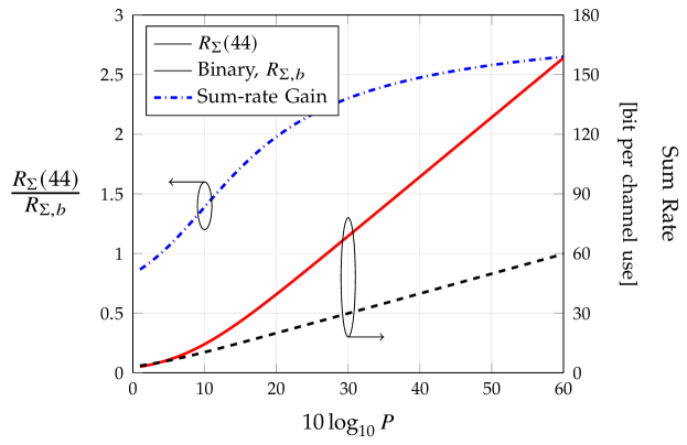
Figure 9: Sum rates achieved in the network depicted in Figure 6 for $K=9$ with two power control strategies: the GDoF-optimal power allocation scheme from (43) is used as a proxy for optimal power control and yields the red solid curve, denoted as $R_{\Sigma}\eqref{eq:KKpwr}$, while the optimal binary power control scheme yields the black dashed curve, denoted as $R_{\Sigma,b}$. Their performance gap is quantified with the sum-rate gain $\left.R_{\Sigma}\eqref{eq:KKpwr}\middle/R_{\Sigma,b}\right.$ (blue dot-dashed curve).

References

- [1] R. H. Etkin, D. N. C. Tse, and H. Wang, “Gaussian interference channel capacity to within one bit,” IEEE Transactions on Information Theory, vol. 54, pp. 5534–5562, Dec 2008.
- [2] Y.-C. Chan, J. Wang, and S. A. Jafar, “Toward an extremal network theory – robust GDoF gain of transmitter cooperation over TIN,” IEEE Transactions on Information Theory, vol. 66, no. 6, pp. 3827–3845, 2020.
- [3] Y.-C. Chan, C. Geng, and S. A. Jafar, “Robust optimality of secure TIN,” IEEE Transactions on Wireless Communications, 2022.
- [4] H. Joudeh and G. Caire, “Cellular networks with finite precision CSIT: GDoF optimality of multi-cell TIN and extremal gains of multi-cell cooperation,” IEEE Transactions on Information Theory, pp. 1–1, 2021.
- [5] M. Chiang, P. Hande, T. Lan, C. W. Tan, et al., “Power control in wireless cellular networks,” Foundations and Trends® in Networking, vol. 2, pp. 381–533, Jun. 2008.
- [6] J. Zander, “Performance of optimum transmitter power control in cellular radio systems,” IEEE transactions on vehicular technology, vol. 41, pp. 57–62, Feb. 1992.
- [7] J. Zander, “Distributed cochannel interference control in cellular radio systems,” IEEE transactions on vehicular Technology, vol. 41, pp. 305–311, Aug. 1992.
- [8] G. J. Foschini and Z. Miljanic, “A simple distributed autonomous power control algorithm and its convergence,” IEEE transactions on vehicular Technology, vol. 42, pp. 641–646, Nov. 1993.
- [9] R. D. Yates, “A framework for uplink power control in cellular radio systems,” IEEE Journal on selected areas in communications, vol. 13, pp. 1341–1347, Sep. 1995.
- [10] N. Bambos, S. C. Chen, and G. J. Pottie, “Channel access algorithms with active link protection for wireless communication networks with power control,” IEEE/ACM Transactions on Networking, vol. 8, pp. 583–597, Oct 2000.
- [11] T. S. Han and K. Kobayashi, “A new achievable rate region for the interference channel,” IEEE Transactions on Information Theory, vol. 27, no. 1, pp. 49–60, 1981.
- [12] H. Joudeh and B. Clerckx, “Sum-rate maximization for linearly precoded downlink multiuser MISO systems with partial CSIT: A rate-splitting approach,” IEEE Transactions on Communications, vol. 64, no. 11, pp. 4847–4861, 2016.
- [13] S. A. Jafar and S. Vishwanath, “Generalized degrees of freedom of the symmetric gaussian user interference channel,” IEEE Transactions on Information Theory, vol. 56, no. 7, pp. 3297–3303, 2010.
- [14] G. Bresler, A. Parekh, and D. N. C. Tse, “The approximate capacity of the many-to-one and one-to-many Gaussian interference channels,” IEEE Transactions on Information Theory, vol. 56, no. 9, pp. 4566–4592, 2010.
- [15] S. A. Jafar, “Interference alignment—a new look at signal dimensions in a communication network,” Foundations and Trends® in Communications and Information Theory, vol. 7, no. 1, pp. 1–134, 2011.
- [16] G. R. Hiertz, D. Denteneer, L. Stibor, Y. Zang, X. P. Costa, and B. Walke, “The IEEE 802.11 universe,” IEEE Communications Magazine, vol. 48, no. 1, pp. 62–70, 2010.
- [17] J. B. Rao and A. O. Fapojuwo, “A survey of energy efficient resource management techniques for multicell cellular networks,” IEEE Communications Surveys & Tutorials, vol. 16, no. 1, pp. 154–180, 2013.
- [18] P. Mach, Z. Becvar, and T. Vanek, “In-band device-to-device communication in OFDMA cellular networks: A survey and challenges,” IEEE Communications Surveys & Tutorials, vol. 17, no. 4, pp. 1885–1922, 2015.
- [19] M. H. C. Garcia, A. Molina-Galan, M. Boban, J. Gozalvez, B. Coll-Perales, T. Şahin, and A. Kousaridas, “A tutorial on 5G NR V2X communications,” IEEE Communications Surveys & Tutorials, 2021.
- [20] B. Li, Z. Fei, and Y. Zhang, “UAV communications for 5G and beyond: Recent advances and future trends,” IEEE Internet of Things Journal, vol. 6, no. 2, pp. 2241–2263, 2019.
- [21] Z. Q. Luo and S. Zhang, “Dynamic spectrum management: Complexity and duality,” IEEE Journal of Selected Topics in Signal Processing, vol. 2, pp. 57–73, Feb 2008.
- [22] L. P. Qian, Y. J. Zhang, and J. Huang, “MAPEL: Achieving global optimality for a non-convex wireless power control problem,” IEEE Transactions on Wireless Communications, vol. 8, no. 3, pp. 1553–1563, 2009.
- [23] C. W. Tan, M. Chiang, and R. Srikant, “Fast algorithms and performance bounds for sum rate maximization in wireless networks,” IEEE/ACM Transactions on Networking, vol. 21, pp. 706–719, June 2013.
- [24] W. Yu and J. Cioffi, “FDMA capacity of Gaussian multiple-access channels with ISI,” IEEE Transactions on Communications, vol. 50, no. 1, pp. 102–111, 2002.
- [25] J. Papandriopoulos and J. S. Evans, “SCALE: A low-complexity distributed protocol for spectrum balancing in multiuser DSL networks,” IEEE Transactions on Information Theory, vol. 55, no. 8, pp. 3711–3724, 2009.
- [26] F. Meshkati, H. V. Poor, and S. C. Schwartz, “Energy-efficient resource allocation in wireless networks,” IEEE Signal Processing Magazine, vol. 24, pp. 58–68, May 2007.
- [27] M. Chiang, C. W. Tan, D. P. Palomar, D. O’neill, and D. Julian, “Power control by geometric programming,” IEEE Transactions on Wireless Communications, vol. 6, pp. 2640–2651, July 2007.
- [28] Q. Shi, M. Razaviyayn, Z.-Q. Luo, and C. He, “An iteratively weighted MMSE approach to distributed sum-utility maximization for a MIMO interfering broadcast channel,” IEEE Transactions on Signal Processing, vol. 59, no. 9, pp. 4331–4340, 2011.
- [29] K. Shen and W. Yu, “Fractional programming for communication systems—part I: Power control and beamforming,” IEEE Transactions on Signal Processing, vol. 66, no. 10, pp. 2616–2630, 2018.
- [30] H. Sun, X. Chen, Q. Shi, M. Hong, X. Fu, and N. D. Sidiropoulos, “Learning to optimize: Training deep neural networks for interference management,” IEEE Transactions on Signal Processing, vol. 66, no. 20, pp. 5438–5453, 2018.
- [31] F. Liang, C. Shen, W. Yu, and F. Wu, “Towards optimal power control via ensembling deep neural networks,” IEEE Transactions on Communications, vol. 68, no. 3, pp. 1760–1776, 2020.
- [32] W. Lee, M. Kim, and D.-H. Cho, “Deep power control: Transmit power control scheme based on convolutional neural network,” IEEE Communications Letters, vol. 22, no. 6, pp. 1276–1279, 2018.
- [33] M. Eisen, C. Zhang, L. F. O. Chamon, D. D. Lee, and A. Ribeiro, “Learning optimal resource allocations in wireless systems,” IEEE Transactions on Signal Processing, vol. 67, no. 10, pp. 2775–2790, 2019.
- [34] Y. Shen, Y. Shi, J. Zhang, and K. B. Letaief, “A Graph Neural Network Approach for Scalable Wireless Power Control,” arXiv e-prints, p. arXiv:1907.08487, July 2019.
- [35] M. Ebrahimi, M. A. Maddah-ali, and A. K. Khandani, “Power allocation and asymptotic achievable sum-rates in single-hop wireless networks,” in 2006 40th Annual Conference on Information Sciences and Systems, pp. 498–503, March 2006.
- [36] A. Gjendemsjø, D. Gesbert, G. E. Øien, and S. G. Kiani, “Binary power control for sum rate maximization over multiple interfering links,” IEEE Transactions on Wireless Communications, vol. 7, pp. 3164–3173, August 2008.
- [37] S. R. Bhaskaran, S. V. Hanly, N. Badruddin, and J. S. Evans, “Maximizing the sum rate in symmetric networks of interfering links,” IEEE Transactions on Information Theory, vol. 56, pp. 4471–4487, Sept 2010.
- [38] M. A. Charafeddine, A. Sezgin, Z. Han, and A. Paulraj, “Achievable and crystallized rate regions of the interference channel with interference as noise,” IEEE Transactions on Wireless Communications, vol. 11, pp. 1100–1111, March 2012.
- [39] L. P. Qian and Y. J. Zhang, “S-MAPEL: Monotonic optimization for non-convex joint power control and scheduling problems,” IEEE Transactions on Wireless Communications, vol. 9, no. 5, pp. 1708–1719, 2010.
- [40] I. C. Paschalidis, F. Huang, and W. Lai, “A message-passing algorithm for wireless network scheduling,” IEEE/ACM Transactions on Networking, vol. 23, no. 5, pp. 1528–1541, 2015.
- [41] X. Wu, S. Tavildar, S. Shakkottai, T. Richardson, J. Li, R. Laroia, and A. Jovicic, “FlashLinQ: A synchronous distributed scheduler for peer-to-peer ad hoc networks,” IEEE/ACM Transactions on Networking, vol. 21, no. 4, pp. 1215–1228, 2013.
- [42] M. Kiamari, C. Wang, A. S. Avestimehr, and H. Papadopoulos, “SINR-threshold scheduling with binary power control for D2D networks,” in GLOBECOM 2017 - 2017 IEEE Global Communications Conference, pp. 1–7, 2017.
- [43] N. Naderializadeh and A. S. Avestimehr, “ITLinQ: A new approach for spectrum sharing in device-to-device communication systems,” IEEE Journal on Selected Areas in Communications, vol. 32, no. 6, pp. 1139–1151, 2014.
- [44] X. Yi and G. Caire, “ITLinQ: An improved spectrum sharing mechanism for device-to-device communications,” 49th Asilomar Conference on Signals, Systems and Computers, pp. 1310 – 1314, 2015.
- [45] K. Shen and W. Yu, “FPLinQ: A cooperative spectrum sharing strategy for device-to-device communications,” in 2017 IEEE International Symposium on Information Theory (ISIT), pp. 2323–2327, 2017.
- [46] M. Lee, G. Yu, and G. Y. Li, “Graph embedding-based wireless link scheduling with few training samples,” IEEE Transactions on Wireless Communications, vol. 20, no. 4, pp. 2282–2294, 2021.
- [47] W. Cui, K. Shen, and W. Yu, “Spatial deep learning for wireless scheduling,” IEEE Journal on Selected Areas in Communications, vol. 37, no. 6, pp. 1248–1261, 2019.
- [48] Z. Zhao, G. Verma, C. Rao, A. Swami, and S. Segarra, “Distributed scheduling using graph neural networks,” in ICASSP 2021 - 2021 IEEE International Conference on Acoustics, Speech and Signal Processing (ICASSP), pp. 4720–4724, 2021.
- [49] H. Inaltekin and S. V. Hanly, “Optimality of binary power control for the single cell uplink,” IEEE Transactions on Information Theory, vol. 58, no. 10, pp. 6484–6498, 2012.
- [50] S. Dayarathna, R. Senanayake, and J. Evans, “Binary power optimality for two link full-duplex network,” in 2020 IEEE Wireless Communications and Networking Conference (WCNC), pp. 1–6, 2020.
- [51] Y. Zhao and G. J. Pottie, “Optimal spectrum management in multiuser interference channels,” IEEE Transactions on Information Theory, vol. 59, no. 8, pp. 4961–4976, 2013.
- [52] N. Badruddin, J. Evans, and S. V. Hanly, “Binary power allocation in symmetric Wyner-type interference networks,” IEEE Transactions on Wireless Communications, vol. 13, pp. 6903–6914, Dec 2014.
- [53] A. Bedekar, S. Borst, K. Ramanan, P. Whiting, and E. Yeh, “Downlink scheduling in CDMA data networks,” in Global Telecommunications Conference, 1999. GLOBECOM ’99, vol. 5, pp. 2653–2657 vol.5, 1999.
- [54] H. ElSawy, A. Sultan-Salem, M.-S. Alouini, and M. Z. Win, “Modeling and analysis of cellular networks using stochastic geometry: A tutorial,” IEEE Communications Surveys & Tutorials, vol. 19, no. 1, pp. 167–203, 2016.
- [55] H. Min, J. Lee, S. Park, and D. Hong, “Capacity enhancement using an interference limited area for device-to-device uplink underlaying cellular networks,” IEEE Transactions on Wireless Communications, vol. 10, no. 12, pp. 3995–4000, 2011.
- [56] X. Lin, J. G. Andrews, and A. Ghosh, “Spectrum sharing for device-to-device communication in cellular networks,” IEEE Transactions on Wireless Communications, vol. 13, no. 12, pp. 6727–6740, 2014.
- [57] Y. Wu, J. Wang, L. Qian, and R. Schober, “Optimal power control for energy efficient D2D communication and its distributed implementation,” IEEE Communications Letters, vol. 19, no. 5, pp. 815–818, 2015.
- [58] G. George, R. K. Mungara, and A. Lozano, “An analytical framework for device-to-device communication in cellular networks,” IEEE Transactions on Wireless Communications, vol. 14, no. 11, pp. 6297–6310, 2015.
- [59] C. Geng, N. Naderializadeh, A. S. Avestimehr, and S. A. Jafar, “On the optimality of treating interference as noise,” IEEE Transactions on Information Theory, vol. 61, pp. 1753–1767, April 2015.
- [60] X. Yi and G. Caire, “Optimality of treating interference as noise: A combinatorial perspective,” IEEE Transactions on Information Theory, vol. 62, pp. 4654–4673, Aug 2016.
- [61] C. Geng and S. A. Jafar, “On the optimality of treating interference as noise: Compound interference networks,” IEEE Transactions on Information Theory, vol. 62, pp. 4630–4653, Aug 2016.
- [62] C. Geng and S. A. Jafar, “Power control by GDoF duality of treating interference as noise,” IEEE Communications Letters, vol. 22, no. 2, pp. 244–247, 2018.
- [63] C. Geng, H. Sun, and S. A. Jafar, “Multilevel topological interference management: A TIM-TIN perspective,” IEEE Transactions on Communications, vol. 69, no. 11, pp. 7350–7362, 2021.