Discrete-Time System of an Intracellular Delayed HIV Model with CTL Immune Response

Abstract

In [Math. Comput. Sci. 12 (2018), no. 2, 111–127], a delayed model describing the dynamics of the Human Immunodeficiency Virus (HIV) with Cytotoxic T Lymphocytes (CTL) immune response is investigated by Allali, Harroudi and Torres. Here, we propose a discrete-time version of that model, which includes four nonlinear difference equations describing the evolution of uninfected, infected, free HIV viruses, and CTL immune response cells and includes intracellular delay. Using suitable Lyapunov functions, we prove the global stability of the disease free equilibrium point and of the two endemic equilibrium points. We finalize by making some simulations and showing, numerically, the consistence of the obtained theoretical results.

1 Introduction

Several mathematical models have been developed to better understand the dynamics of the HIV disease [4, 10, 15, 17]. Human immunodeficiency virus (HIV) causes acquired immunodeficiency syndrome (AIDS), which is considered the end-stage of the infection. In this stage, the immune system fails to protect the whole body against harmful intruders. This happens because of the destruction of most of CD4+ T cells by the HIV virus, reducing them to fewer than 200 cells [2, 25]. Among available mathematical models, in [21] HIV and tuberculosis coinfection is investigated. A particular case, using real data from Cape Verde islands, has been carried out in [22], while the discrete case was analyzed in [24], showing that ending AIDS epidemic by 2030 is a nontrivial task. Several models introduce the effect of cellular immune response, also called the cytotoxic T-lymphocyte (CTL) response, which attacks and kills the infected cells, see, for instance, [6, 19, 23]. The models show that this cellular immune response can control the load of HIV viruses. In [5], it is assumed that CTL proliferation depends, besides infected cells, as usual, also on healthy cells. Recently, the same problem was tackled by introducing time delays [7, 19], which is justified by the fact that uninfected cells must be in contact with the HIV virus before they become infected. In [1], the investigation continued and the proposed basic model, illustrating this type of scenario, is

$$\begin{cases}\dot{X}(t)=\lambda-dX(t)-\beta X(t)V(t),\\[5.69046pt] \dot{Y}(t)=\beta X(t)V(t)-aY(t)-pY(t)Z(t),\\[5.69046pt] \dot{V}(t)=aNY(t)-\mu V(t),\\[5.69046pt] \dot{Z}(t)=cX(t)Y(t)Z(t)-sZ(t),\end{cases}$$ (1)

with given initial conditions $X(0)=X_{0}$, $Y(0)=Y_{0}$, $V(0)=V_{0}$, and $Z(0)=Z_{0}$. In this model (1), $X(t)$, $Y(t)$, $V(t)$ and $Z(t)$ denote, respectively, the concentrations at time $t$ of uninfected cells, infected cells, HIV virus, and CTL cells. The healthy CD4+ cells grow at a rate $\lambda$, decay at a rate $dX(t)$, and become infected by the virus at a rate $\beta X(t)V(t)$. Infected cells $Y$ die at a rate $a$ and are killed by the CTL response at a rate $p$. Free virus $V$ is produced by the infected cells at a rate a $N$ and decay at a rate $\mu$, where $N$ is the number of free virus produced by each actively infected cell during its life time. Finally, CTLs $Z$ expand in response to viral antigen derived from infected cells at a rate $c$ and decay in the absence of antigenic stimulation at a rate $s$. Our starting point here will be an extension of the continuous model (1), composed by nonlinear delayed ordinary differential equations. For most of these types of systems we cannot find the exact analytical solution. To perform numerical simulations using digital computers, we need to discretize the systems [8]. There are several methods that allow us to discretize a model. One that has presented interesting results, and that we use here, is the nonstandard finite discrete difference (NSFD) scheme of Mickens [11, 12, 13, 14].

Our work is organized as follows. Section 2 is devoted to the delayed version of the continuous model (1), presenting its equilibrium points and available results about their stability. Section 3 is dedicated to the presentation of our discrete model and the proof of existence, positivity and boundedness of solutions. We end the section by proving the global stability of the equilibrium points, using suitable Lyapunov functions, followed by some numerical simulations. Finally, conclusions are given in Section 4.

2 Preliminaries

We start by presenting the continuous-time model with delays that serves as the basis of our current work, as well as results regarding the stability of its equilibrium points.

In order to be realistic, in [1] it has been introduced an intracellular time delay to the system of equations (1). Then, the model takes the following form:

$$\begin{cases}\dot{X}(t)=\lambda-dX(t)-\beta X(t)V(t),\\[5.69046pt] \dot{Y}(t)=\beta X(t-\tau)V(t-\tau)-aY(t)-pY(t)Z(t),\\[5.69046pt] \dot{V}(t)=aNY(t)-\mu V(t),\\[5.69046pt] \dot{Z}(t)=cX(t)Y(t)Z(t)-sZ(t).\end{cases}$$ (2)

Here, the delay $\tau$ represents the time needed for infected cells to produce virions after viral entry. The model (2) is a system of delayed ordinary differential equations. For such kind of problems, initial functions need to be addressed and an appropriate functional framework needs to be specified. Following [1], we consider the Banach space $X=C([-\tau,0];\mathbbm{R}^{4})$ of continuous mappings from $[-\tau,0]$ to $\mathbbm{R}^{4}$, equipped with the sup-norm $\|\phi\|=\underset{-\tau\leq t\leq 0}{\sup}|\phi(t)|$. It is assumed that the initial functions verify $(X(\theta),Y(\theta),V(\theta),Z(\theta))\in X$. Also, from biological reasons, these initial functions $X(\theta)$, $Y(\theta)$, $V(\theta)$ and $Z(\theta)$ have to be nonnegative: $X(\theta)\geq 0$, $Y(\theta)\geq 0$, $V(\theta)\geq 0$, $Z(\theta)\geq 0$, for $\theta\in[-\tau,0]$. In Theorem 1 of [1] it is proved that any solution of this system, satisfying certain conditions, is nonnegative and bounded for all $\tau\geq 0$. Moreover, the continuous model has three equilibrium points:

$$E_{0}=\left(\dfrac{\lambda}{d},0,0,0\right)$$

and two endemic equilibrium points given by

$$E^{\ast}=\left(\dfrac{\mu}{N\beta},\dfrac{\lambda\beta N-d\mu}{aN\beta},\dfrac{\lambda\beta N-d\mu}{\mu\beta},0\right)$$

and

$$\overline{E}=\left(\dfrac{\lambda\mu c-\beta aNs}{d\mu c},\dfrac{ds\mu}{\lambda\mu c-\beta aNs},\dfrac{dsaN}{\lambda\mu c-\beta aNs},\frac{\beta aN}{\mu p}\left(\dfrac{\lambda\mu c-\beta aNs}{d\mu c}\right)-\dfrac{a}{p}\right).$$

Regarding the stability of the disease-free equilibrium $E_{0}$, the following result was proved.

Theorem 2.1 (See Theorem 2 of [1]).

The local stability of the disease-free equilibrium point depends on the value $N\beta\lambda-d\mu$. Precisely,

1. if $N\beta\lambda-d\mu<0$, then the disease-free equilibrium point $E_{0}$ is locally asymptotically stable for any time delay $\tau\geq 0$;

2. if $N\beta\lambda-d\mu>0$, then the equilibrium $E_{0}$ is unstable for any time delay $\tau\geq 0$.

For the local stability of the infected-equilibrium $E^{\ast}$, the following result holds.

Theorem 2.2 (See Theorem 3 of [1]).

The local stability of the disease-free equilibrium $E^{\ast}$ depends on the value of $\beta N(\mu c\lambda-\beta saN)-\mu^{2}cd$. Precisely,

1. if $\beta N(\mu c\lambda-\beta saN)-\mu^{2}cd<0$, then $E^{\ast}$ is locally asymptotically stable for any positive time delay;

2. if $\beta N(\mu c\lambda-\beta saN)-\mu^{2}cd>0$, then $E^{\ast}$ is unstable for any time delay.

For the second endemic equilibrium point $\overline{E}$, the following result has been proved.

Theorem 2.3 (See Theorem 4 of [1]).

Assume that $\mu c\lambda-\beta saN>0$. If $\beta N(\mu c\lambda-\beta saN)-\mu^{2}cd>0$, then the infected equilibrium point $\overline{E}$ is locally asymptotically stable for $\tau=0$.

For $\tau>0$, the stability of $\overline{E}$ remains open. Here we provide, for the first time in the literature, a proper discrete-time version of the HIV model (2).

3 Main Results

We begin this section by presenting our discrete-time model. Afterwards, we show the well-posedness of the model, that is, we prove that its solutions are positive and bounded. Moreover, we show that the equilibrium points are the same of the continuous model. We finalize this section by proving the global stability of each equilibrium point. For that we use suitable Lyapunov functions. We end this section by presenting some numerical simulations, which show consistence with the obtained theoretical results.

3.1 The discrete-time model

One of the important features of the discrete-time epidemic models obtained by Mickens’ method is that they present the same features as the corresponding original continuous-time models. Here, we construct a dynamically consistent numerical NSFD scheme for solving (2) based on [11, 12, 13, 14]. Let us define the time instants $t_{n}=nh$ with $n$ integer, the step size as $h=t_{n+1}-t_{n}$, and $(X_{n},V_{n},Y_{n},Z_{n})$ as the approximated values of $(X(nh),V(nh),Y(nh),Z(nh))$.

Discretizing system (2) using the NSFD scheme, we obtain:

$$\begin{cases}\dfrac{X_{n+1}-X_{n}}{\phi(h)}=\lambda-dX_{n+1}-\beta X_{n+1}V_{n},\\[5.69046pt] \dfrac{Y_{n+1}-Y_{n}}{\phi(h)}=\beta X_{n-m+1}V_{n-m}-aY_{n+1}-pY_{n+1}Z_{n},\\[5.69046pt] \dfrac{V_{n+1}-V_{n}}{\phi(h)}=aNY_{n+1}-\mu V_{n+1},\\[5.69046pt] \dfrac{Z_{n+1}-Z_{n}}{\phi(h)}=cX_{n}Y_{n+1}Z_{n}-sZ_{n+1},\end{cases}$$ (3)

where the denominator function is $\phi(h)=h$ [7, 14]. Throughout our study, for brevity, we write $\phi(h)=\phi$. Let us assume that there exists an integer $m\in\mathbbm{N}$ with $\tau=m\phi$. The initial conditions of system (3) are

$$X_{k}=\psi_{k}^{1}\geq 0;\quad Y_{k}=\psi_{k}^{2}\geq 0;\quad V_{k}=\psi_{k}^{3}\geq 0;\quad Z_{k}=\psi_{k}^{4}\geq 0$$ (4)

for all $k=-m,-m+1,\ldots,0$ and $\psi_{0}^{i}>0$, $i=1,2,3,4$.

Define the region

$$\Gamma=\left\{(x,y,v,z):0<X_{n},Y_{n},V_{n}\leq N_{1},Z_{n}<N_{2}\right\},$$

where $N_{1}=\dfrac{aN\lambda}{Q}$, $Q=\min\{d,\frac{a}{2},\mu\}$ and $N_{2}=\dfrac{cX_{n}\beta X_{n-m+1}V_{n-m}}{ps}$.

Lemma 3.1.

Any solution $(X_{n},Y_{n},V_{n},Z_{n})$ of model (3) with initial conditions (4) is positive and ultimately bounded.

Proof 3.2.

Since model (3) is linear in $X_{n+1}$, $Y_{n+1}$, $V_{n+1}$, and $Z_{n+1}$, we can rewrite it as

$$\begin{cases}X_{n+1}=\dfrac{\lambda\phi+X_{n}}{1+d\phi+\beta\phi V_{n}},\\[8.5359pt] Y_{n+1}=\dfrac{Y_{n}+\beta\phi X_{n-m+1}Y_{n-m}}{1+a\phi+p\phi Z_{n}},\\[8.5359pt] V_{n+1}=\dfrac{V_{n}+aN\phi Y_{n+1}}{1+\mu\phi},\\[8.5359pt] Z_{n+1}=\dfrac{Z_{n}+c\phi X_{n}Y_{n+1}Z_{n}}{1+s\phi}.\end{cases}$$ (5)

Since all the parameters of model (3) and the initial conditions are positive, it follows, by induction, that $X_{n}\geq 0$, $Y_{n}\geq 0$, $V_{n}\geq 0$, and $Z_{n}\geq 0$, for all $n\in\mathbbm{N}$. Regarding the boundedness of the solutions, let

$$\Omega_{n}=aNX_{n}+aNY_{n+m}+\frac{a}{2}V_{n+m},$$ (6)

from which

$$\Omega_{n+1}-\Omega_{n} =aN(X_{n+1}-X_{n})+aN(Y_{n+m+1}-Y_{n+m})+\frac{a}{2}(V_{n+m+1}-V_{n+m})$$

$$=aN\phi(\lambda-dX_{n+1}-\beta X_{n+1}V_{n})+aN\phi(\beta X_{n+1}V_{n}-aY_{n+m+1}$$

$$\quad-pY_{n+m+1}Z_{n+m})+\frac{a}{2}\phi(aNY_{n+m+1}-\mu V_{n+m+1})$$

$$=aN\lambda\phi-aNd\phi X_{n+1}-\frac{a^{2}}{2}\phi NY_{n+m+1}-aNp\phi Y_{n+\tau+1}Z_{n+\tau}$$

$$\quad-\frac{a}{2}\mu\phi V_{n+m+1}.$$

Set $Q=\min\{d,\frac{a}{2},\mu\}$. Then,

$$\Omega_{n+1}-\Omega_{n}\leq aN\lambda\phi-Q\phi\Omega_{n+1}$$

so that $\Omega_{n+1}(1+Q\phi)\leq aN\lambda\phi+\Omega_{n}$. Hence, by [20],

$$\Omega_{n+1}\leq\dfrac{aN\lambda\phi}{1+Q\phi}+\dfrac{\Omega_{n}}{1+Q\phi}$$

and

$$\Omega_{n}\leq\left(\dfrac{1}{1+Q\phi}\right)^{n}\Omega_{0}+\dfrac{aN\lambda}{Q}\left(1-\left(\frac{1}{1+Q\phi}\right)^{n}\right)$$ (7)

so that $\underset{n\to\infty}{\limsup}\,\Omega_{n}\leq\dfrac{aN\lambda}{Q}=N_{1}$. Therefore, $\underset{n\to\infty}{\limsup}X_{n}\leq N_{1}$, $\underset{n\to\infty}{\limsup}Y_{n}\leq N_{1}$, and $\underset{n\to\infty}{\limsup}V_{n}\leq N_{1}$. From the second and last equation of system (3) we have

$$Z_{n+1}-Z_{n}=c\phi X_{n}Y_{n+1}Z_{n}-s\phi Z_{n+1}$$

or

$$Z_{n+1}-Z_{n} =c\phi X_{n}\left(\beta X_{n-m+1}V_{n-m}-aY_{n+1}-\frac{(Y_{n+1}+Y_{n})}{\phi}\right)-s\phi Z_{n+1}$$

$$\leq\frac{c\phi X_{n}\beta X_{n-m+1}V_{n-m}}{p}-s\phi Z_{n+1}.$$

It follows from [20] that

$$Z_{n+1} \leq\frac{\frac{c\phi X_{n}\beta X_{n-m+1}V_{n-m}}{p}}{1+s\phi}+\frac{Z_{n}}{1+s\phi}$$

$$\leq\left(\dfrac{1}{1+s\phi}\right)^{n+1}Z_{0}+\frac{cX_{n}\beta X_{n-m+1}V_{n-m}}{ps}\left(1-\left(\frac{1}{1+s\phi}\right)^{n+1}\right).$$

Consequently,

$$Z_{n}\leq\frac{cX_{n}(\beta X_{n-m+1}V_{n-m})}{p\ s}=N_{2}$$

and every local solution $(X_{n},Y_{n},V_{n},Z_{n})$ tends to $\Gamma$ as $n\to\infty$. ∎

System (3) has three equilibria:

1. the disease free equilibrium point $E_{0}=\left(\frac{\lambda}{d},0,0,0\right)$;

2. the persistent infection equilibrium point without immune response,

   $$E^{\ast}=\left(\frac{\mu}{\beta N},\frac{\beta N\lambda-d\mu}{\beta Na},\frac{\beta N\lambda-d\mu}{\beta\mu},0\right);$$

3. the persistent infection equilibrium with immune response,

$$\overline{E}=\left(\frac{\lambda c\mu-\beta saN}{dc\mu},\frac{d\mu s}{\lambda c\mu-\beta saN},\frac{saNd}{\lambda c\mu-\beta saN},\frac{\beta aN(\lambda c\mu-\beta saN)-adc\mu^{2}}{pdc\mu^{2}}\right).$$

The equilibrium point $E^{\ast}$ only exists if $\beta N\lambda-d\mu>0$, so let us define the basic reproduction number as

$$\mathcal{R}_{0}:=\frac{\beta N\lambda}{d\mu}.$$

The equilibrium $\overline{E}$ only exists if $\beta aN(\lambda c\mu-\beta saN)-adc\mu^{2}>0$, so let us set the humoural immune response reproduction number as

$$\mathcal{R}_{1}:=\dfrac{\beta N(\lambda c\mu-\beta saN)}{dc\mu^{2}}.$$

Clearly,

$$\mathcal{R}_{1}=\dfrac{\mathcal{R}_{0}(\lambda c\mu-\beta saN)}{\lambda c\mu}<\mathcal{R}_{0}.$$

We can express the equilibrium points in terms of $\mathcal{R}_{0}$ and $\mathcal{R}_{1}$ as follows:

$$E_{0} =(X_{0},V_{0},V_{0},Z_{0})=\left(\frac{\lambda}{d},0,0,0\right),$$

$$E^{\ast} =(X^{\ast},Y^{\ast},V^{\ast},Z^{\ast})=\left(\frac{X_{0}}{\mathcal{R}_{0}},\frac{\lambda}{a\mathcal{R}_{0}}(\mathcal{R}_{0}-1),\frac{N\lambda}{\mu\mathcal{R}_{0}}(\mathcal{R}_{0}-1),0\right),$$

$$\overline{E} =(\overline{X},\overline{Y},\overline{V},\overline{Z})=\left(\frac{\mathcal{R}_{1}\mu}{\beta N},\frac{s\beta N}{\mu c\mathcal{R}_{1}},\frac{\beta N^{2}as}{\mu^{2}c\mathcal{R}_{1}},\frac{a(\mathcal{R}_{1}-1)}{p}\right).$$

We can see from the previous relations that $E^{\ast}$ exists when $\mathcal{R}_{1}<1<\mathcal{R}_{0}$ and $\overline{E}$ only exists if $\mathcal{R}_{0}>\mathcal{R}_{1}>1$.

3.2 Global stability

In this section, we prove the global stability of all the equilibria using suitable Lyapunov functions. We use the function $G(x)=x-\ln(x)-1$ that is positive for all $x>0$ and $G(1)=0$. We make also use of the basic inequality

$$\ln(x)\leq x-1.$$ (8)

Theorem 3.3.

Suppose that $\mathcal{R}_{0}\leq 1$. Then $E_{0}$ of model (3) is globally asymptotically stable.

Proof 3.4.

Define the discrete Lyapunov function $L_{n}$ as

$$L_{n}(X_{n},Y_{n},V_{n},Z_{n}) =\frac{1}{\phi}\left(X_{0}G\left(\frac{X_{n}}{X_{0}}\right)+Y_{n}+\frac{1+\mu\phi}{N}V_{n}+\frac{p}{cN_{1}}(1+s\phi)Z_{n}\right)$$

$$\qquad+\sum_{j=n-m}^{n-1}\beta X_{j+1}V_{j}.$$

It follows that $L_{n}(X_{n},Y_{n},V_{n},Z_{n})>0$ for all $X_{n}\geq 0$, $Y_{n}\geq 0$, $V_{n}\geq 0$ and $Z_{n}\geq 0$. Moreover, $L_{n}(X_{n},Y_{n},V_{n},Z_{n})=0$ if $(X_{n},Y_{n},V_{n},Z_{n})=E_{0}$. Computing $\Delta L_{n}=L_{n+1}-L_{n}$, we have

$$\Delta L_{n}=\frac{1}{\phi}\left(X_{0}G\left(\frac{X_{n+1}}{X_{0}}\right)+Y_{n+1}+\frac{1+\mu\phi}{N}V_{n+1}+\frac{p}{cN_{1}}(1+s\phi)Z_{n+1}\right)$$

$$+\sum_{j=n-m+1}^{n}\beta X_{j+1}V_{j}$$

$$-\left[\frac{1}{\phi}\left(X_{0}G\left(\frac{X_{n}}{X_{0}}\right)+Y_{n}+\frac{1+\mu\phi}{N}V_{n}+\frac{p}{cN_{1}}(1+s\phi)Z_{n}\right)+\sum_{j=n-m}^{n-1}\beta X_{j+1}V_{j}\right]$$

$$=\frac{1}{\phi}\left[X_{0}\left(\frac{X_{n+1}}{X_{0}}-\frac{X_{n}}{X_{0}}+\ln\left(\frac{X_{n}}{X_{n+1}}\right)\right)+(Y_{n+1}-Y_{n})+\frac{1+\mu\phi}{N}(V_{n+1}-V_{n})\right]$$

$$+\frac{1}{\phi}\left[\frac{p}{cN_{1}}(1+s\phi)(Z_{n+1}-Z_{n})\right]+\beta\left(\sum_{j=n-m+1}^{n}X_{j+1}V_{j}-\sum_{j=n-m}^{n-1}X_{j+1}V_{j}\right).$$

Using (8), we have

$$\Delta L_{n}\leq\frac{1}{\phi}\left[\left(1-\frac{X_{0}}{X_{n+1}}\right)\left(X_{n+1}-X_{n}\right)+(Y_{n+1}-Y_{n})+\frac{1+\mu\phi}{N}(V_{n+1}-V_{n})\right]$$

$$\quad+\frac{1}{\phi}\left[\frac{p}{cN_{1}}(1+s\phi)(Z_{n+1}-Z_{n})\right]+\beta\left(X_{n+1}V_{n}-X_{n-m+1}V_{n-m}\right)$$

$$=\left(1-\frac{X_{0}}{X_{n+1}}\right)\frac{X_{n+1}-X_{n}}{\phi}+\frac{Y_{n+1}-Y_{n}}{\phi}+\frac{V_{n+1}-V_{n}}{N\phi}+\frac{p(Z_{n+1}-Z_{n})}{cN_{1}\phi}$$

$$+\beta\left(\sum_{j=n-m+1}^{n}X_{j+1}V_{j}-\sum_{j=n-m}^{n-1}X_{j+1}V_{j}\right)+\frac{\mu}{N}(V_{n+1}-V_{n})+\frac{ps}{cN_{1}}(Z_{n+1}-Z_{n}).$$

From the equations of system (3),

$$\Delta L_{n} \leq\left(1-\frac{X_{0}}{X_{n+1}}\right)\left(\lambda-dX_{n+1}-\beta X_{n+1}V_{n}\right)$$

$$\quad+(\beta X_{n-m+1}V_{n-m}-aY_{n+1}-pY_{n+1}Z_{n})$$

$$\quad+\frac{1}{N}(aNY_{n+1}-\mu V_{n+1})+\frac{p}{cN_{1}}(cX_{n}Y_{n+1}Z_{n}-sZ_{n+1})$$

$$\quad+\beta\left(X_{n+1}V_{n}-X_{n-m+1}V_{n-m}\right)$$

$$\quad+\frac{\mu}{N}(V_{n+1}-V_{n})+\frac{s\ p}{cN_{1}}(Z_{n+1}-Z_{n})$$

$$=\left(\lambda-dX_{n+1}\right)\left(1-\frac{X_{0}}{X_{n+1}}\right)+\beta X_{0}V_{n}-pY_{n+1}Z_{n}-\frac{\mu}{N}V_{n}$$

$$\quad+\frac{p}{cN_{1}}cX_{n}Y_{n+1}Z_{n}-\frac{s\ p}{cN_{1}}Z_{n}.$$

Using the first equation of (3) at the equilibrium point $E_{0}$,

$$\Delta L_{n} \leq d\left(X_{0}-X_{n+1}\right)\left(1-\frac{X_{0}}{X_{n+1}}\right)+V_{n}\left(\frac{\beta\lambda}{d}-\frac{\mu}{N}\right)+\left(\frac{pX_{n}}{N_{1}}-p\right)Y_{n+1}Z_{n}$$

$$\qquad-\frac{s\ p}{cN_{1}}Z_{n}$$

$$=-\frac{d\left(X_{n+1}-X_{0}\right)^{2}}{X_{n+1}}-\frac{\mu}{N}V_{n}\left(1-\mathcal{R}_{0}\right)-pY_{n+1}Z_{n}\left(1-\frac{X_{n}}{N_{1}}\right)-\frac{s\ p}{cN_{1}}Z_{n}.$$

Since $\mathcal{R}_{0}\leq 1$ and $\underset{n\to\infty}{\lim\sup}X_{n}=N_{1}$, one has $\Delta L_{n}\leq 0$ for all $n\geq 0$, that is, $L_{n}$ is a monotone decreasing sequence. If $L_{n}\geq 0$, then there is a limit for $\underset{n\to\infty}{\lim}L_{n}\geq 0$. Therefore, $\underset{n\to\infty}{\lim}\Delta L_{n}=0$ implies $\underset{n\to\infty}{\lim}X_{n}=X_{0}$ and

$$\underset{n\to\infty}{\lim}Y_{n}=\underset{n\to\infty}{\lim}V_{n}=\underset{n\to\infty}{\lim}Z_{n}=0.$$

So, if $\mathcal{R}_{0}\leq 1$, then $E_{0}$ is globally asymptotically stable. ∎

Lemma 3.5.

If $\mathcal{R}_{1}<1<\mathcal{R}_{0}$, then $Y^{\ast}<\overline{Y}$.

Proof 3.6.

One can easily see that

$$Y^{\ast}-\overline{Y} =\frac{\lambda(\mathcal{R}_{0}-1)}{a\mathcal{R}_{0}}-\frac{\beta sN}{\mu c\mathcal{R}_{1}}=\frac{\lambda\mu c\mathcal{R}_{1}(\mathcal{R}_{0}-1)-as\beta N\mathcal{R}_{0}}{a\mu c\mathcal{R}_{1}\mathcal{R}_{0}}$$

$$<\frac{\lambda\mu c\mathcal{R}_{0}(\mathcal{R}_{0}-1)-as\beta N\mathcal{R}_{0}}{a\mu c\mathcal{R}_{1}\mathcal{R}_{0}}=\frac{\lambda\mu c(\mathcal{R}_{0}-1)-as\beta N}{a\mu c\mathcal{R}_{1}}$$

and $Y^{\ast}-\overline{Y}<0$, that is, $-\lambda\mu c<as\beta N-\lambda\mu c\mathcal{R}_{0}<as\beta N-\lambda\mu c$. The proof is complete. ∎

Theorem 3.7.

If $\mathcal{R}_{1}\leq 1<\mathcal{R}_{0}$, then $E^{\ast}$ is globally asymptotically stable.

Proof 3.8.

Define

$$\mathcal{L}_{n}(X_{n},Y_{n},V_{n},Z_{n})$$

$$=\frac{1}{\phi}\left[X^{\ast}G\left(\frac{X_{n}}{X^{\ast}}\right)+Y^{\ast}G\left(\frac{Y_{n}}{Y^{\ast}}\right)+\frac{(1+\mu\phi)V^{\ast}}{N}G\left(\frac{V_{n}}{V^{\ast}}\right)+\frac{p(1+s\phi)}{cN_{1}}Z_{n}\right]$$

$$\quad+\beta X^{\ast}V^{\ast}\sum_{j=n-m}^{n-1}G\left(\frac{X_{j+1}V_{j}}{X^{\ast}V^{\ast}}\right).$$

Then $\mathcal{L}_{n}(X_{n},Y_{n},V_{n},Z_{n})$ is positive for all $X_{n},Y_{n},V_{n},Z_{n}$ strictly positive and it is equal to zero at $(X^{\ast},Y^{\ast},V^{\ast},Z^{\ast})$. Computing $\Delta\mathcal{L}_{n}=\mathcal{L}_{n+1}-\mathcal{L}_{n}$, we get

$$\Delta\mathcal{L}_{n} =\frac{X^{\ast}}{\phi}G\left(\frac{X_{n+1}}{X^{\ast}}\right)+\frac{Y^{\ast}}{\phi}G\left(\frac{Y_{n+1}}{Y^{\ast}}\right)+\frac{V^{\ast}(1+\mu\phi)}{N\phi}G\left(\frac{V_{n+1}}{V^{\ast}}\right)$$

$$\quad+\frac{p(1+s\phi)}{cN_{1}\phi}Z_{n+1}+\beta X^{\ast}V^{\ast}\sum_{j=n-m+1}^{n}G\left(\frac{X_{j+1}V_{j}}{X^{\ast}V^{\ast}}\right)$$

$$=-\left[\frac{X^{\ast}}{\phi}G\left(\frac{X_{n}}{X^{\ast}}\right)+\frac{Y^{\ast}}{\phi}G\left(\frac{Y_{n}}{Y^{\ast}}\right)+\frac{V^{\ast}(1+\mu\phi)}{N\phi}G\left(\frac{V_{n}}{V^{\ast}}\right)+\frac{p(1+s\phi)}{cN_{1}\phi}Z_{n}\right]$$

$$\quad-\beta X^{\ast}V^{\ast}\sum_{j=n-m}^{n-1}G\left(\frac{X_{j+1}V_{j}}{X^{\ast}V^{\ast}}\right)$$

$$=\frac{1}{\phi}\left(X^{\ast}\left(G\left(\frac{X_{n+1}}{X^{\ast}}\right)-G\left(\frac{X_{n}}{X^{\ast}}\right)\right)+Y^{\ast}\left(G\left(\frac{Y_{n+1}}{Y^{\ast}}\right)-G\left(\frac{Y_{n}}{Y^{\ast}}\right)\right)\right)$$

$$\quad+\frac{1}{\phi}\left(\frac{p(1+s\phi)}{cN_{1}}\left(Z_{n+1}-Z_{n}\right)\right)+\frac{V^{\ast}(1+\mu\phi)}{N}\left(G\left(\frac{V_{n+1}}{V^{\ast}}\right)-G\left(\frac{V_{n}}{V^{\ast}}\right)\right)$$

$$\quad+\beta X^{\ast}V^{\ast}\left(G\left(\frac{X_{n+1}V_{n}}{X^{\ast}V^{\ast}}\right)-G\left(\frac{X_{n-m+1}V_{n-m}}{X^{\ast}V^{\ast}}\right)\right).$$

Recalling inequality (8), we have

$$\begin{split}G\left(\frac{\xi_{n+1}}{\xi^{\ast}}\right)-G\left(\frac{\xi_{n}}{\xi^{\ast}}\right)&=\left(\frac{\xi_{n+1}-\xi_{n}}{\xi^{\ast}}\right)+\ln\left(\frac{\xi_{n}}{\xi_{n+1}}\right)\\ &\leq\left(\xi_{n+1}-\xi_{n}\right)\left(\frac{1}{\xi^{\ast}}-\frac{1}{\xi_{n+1}}\right)\end{split}$$

for $\xi=\{X,Y,V,Z\}$. Therefore,

$$\Delta\mathcal{L}_{n} \leq\frac{1}{\phi}\left(\left(X_{n+1}-X_{n}\right)\left(1-\frac{X^{\ast}}{X_{n+1}}\right)+\left(Y_{n+1}-Y_{n}\right)\left(1-\frac{Y^{\ast}}{Y_{n+1}}\right)\right)$$

$$\quad+\frac{1}{\phi}\left(\frac{1}{N}\left(V_{n+1}-V_{n}\right)\left(1-\frac{V^{\ast}}{V_{n+1}}\right)+\frac{p}{cN_{1}}\left(Z_{n+1}-Z_{n}\right)\right)$$

$$\quad+\frac{\mu V^{\ast}}{N}\left(G\left(\frac{V_{n+1}}{V^{\ast}}\right)-G\left(\frac{V_{n}}{V^{\ast}}\right)\right)+\frac{p\ s}{cN_{1}}(Z_{n+1}-Z_{n})$$

$$\quad+\beta X^{\ast}V^{\ast}\left(\frac{X_{n+1}V_{n}}{X^{\ast}V^{\ast}}-\frac{X_{n-m+1}V_{n-m}}{X^{\ast}V^{\ast}}+\ln\left(\frac{X_{n-m+1}V_{n-m}}{X_{n+1}V_{n}}\right)\right).$$

Using the equations of system (3), we have

$$\Delta\mathcal{L}_{n} \leq\left(\lambda-dX_{n+1}-\beta X_{n+1}V_{n}\right)\left(1-\frac{X^{\ast}}{X_{n+1}}\right)$$

$$\quad+\left(\beta X_{n-m+1}V_{n-m}-aY_{n+1}-pY_{n+1}Z_{n}\right)\left(1-\frac{Y^{\ast}}{Y_{n+1}}\right)$$

$$\quad+\frac{1}{N}\left(aNY_{n+1}-\mu V_{n+1}\right)\left(1-\frac{V^{\ast}}{V_{n+1}}\right)+\frac{p}{cN_{1}}\left(cX_{n}Y_{n+1}Z_{n}-sZ_{n+1}\right)$$

$$\quad+\frac{\mu V^{\ast}}{N}\left(\frac{V_{n+1}}{V^{\ast}}-\frac{V_{n}}{V^{\ast}}+\ln\left(\frac{V_{n}}{V_{n+1}}\right)\right)+\frac{p\ s}{cN_{1}}(Z_{n+1}-Z_{n})$$

$$\quad+\beta X^{\ast}V^{\ast}\left(\frac{X_{n+1}V_{n}}{X^{\ast}V^{\ast}}-\frac{X_{n-m+1}V_{n-m}}{X^{\ast}V^{\ast}}+\ln\left(\frac{X_{n-m+1}V_{n-m}}{X_{n+1}V_{n}}\right)\right).$$

Expanding, simplifying, and using the conditions of system (3) at $E^{\ast}$, where

$$\lambda =dX^{\ast}+\beta X^{\ast}V^{\ast},\qquad\beta X^{\ast}V^{\ast}=aY^{\ast},\qquad aNY^{\ast}=\mu V^{\ast},\qquad X^{\ast}=\frac{\mu}{\beta N},$$

we get

$$\Delta\mathcal{L}_{n} \leq\left(1-\frac{X^{\ast}}{X_{n+1}}\right)(\lambda-dX_{n+1})+\beta X^{\ast}V_{n}-pY_{n+1}Z_{n}+aY^{\ast}$$

$$\quad-\beta X^{\ast}V^{\ast}\frac{X_{n-m+1}V_{n-m}Y^{\ast}}{x^{\ast}V^{\ast}Y_{n+1}}+pY^{\ast}Z_{n}-aY^{\ast}\frac{V^{\ast}Y_{n+1}}{V_{n+1}Y^{\ast}}+\frac{\mu}{N}V^{\ast}$$

$$\quad+\frac{p}{N_{1}}X_{n}Y_{n+1}Z_{n}-\frac{\mu}{N}V_{n}+\frac{\mu}{N}V^{\ast}\ln\left(\frac{V_{n}}{V_{n+1}}\right)-\frac{p\ s}{cN_{1}}Z_{n}$$

$$\quad+\beta X^{\ast}V^{\ast}\ln\left(\frac{X_{n-m+1}V_{n-m}}{X_{n+1}V_{n}}\right)$$

$$\leq-\frac{d(X_{n+1}-X^{\ast})^{2}}{X_{n+1}}-pY_{n+1}Z_{n}\left(1-\frac{X_{n}}{N_{1}}\right)+pZ_{n}\left(Y^{\ast}-\overline{Y}\right)$$

$$\quad+\beta X^{\ast}V^{\ast}\left[3-\frac{X^{\ast}}{X_{n+1}}-\frac{X_{n-m+1}V_{n-m}Y^{\ast}}{X^{\ast}V^{\ast}Y_{n+1}}-\frac{V^{\ast}Y_{n+1}}{V_{n+1}Y^{\ast}}\right.$$

$$\left.\qquad+\ln\left(\frac{X_{n-m+1}V_{n-m}}{X_{n+1}V_{n+1}}\right)\right]$$

$$\leq-\frac{d(X_{n+1}-X^{\ast})^{2}}{X_{n+1}}-pY_{n+1}Z_{n}\left(1-\frac{X_{n}}{N_{1}}\right)+pZ_{n}\left(Y^{\ast}-\overline{Y}\right)$$

$$\quad+\beta X^{\ast}V^{\ast}\left(-G\left(\frac{X^{\ast}}{X_{n+1}}\right)-G\left(\frac{X_{n-m+1}V_{n-m}Y^{\ast}}{X^{\ast}V^{\ast}Y_{n+1}}\right)-G\left(\frac{V^{\ast}Y_{n+1}}{V_{n+1}Y^{\ast}}\right)\right).$$

Hence, if $\mathcal{R}_{1}\leq 1<\mathcal{R}_{0}$, and since $\underset{n\to\infty}{\lim\sup}X_{n}=N_{1}$ and Lemma 3.5 holds, it follows that $\mathcal{L}_{n}$ is a monotone deceasing sequence. Since $\mathcal{L}_{n}\geq 0$, then $\underset{n\to\infty}{\lim}{\mathcal{L}_{n}}\geq 0$. Therefore, $\underset{n\to\infty}{\lim}\Delta\mathcal{L}_{n}=0$, which implies that $\underset{n\to\infty}{\lim}X_{n}=X^{\ast}$ and $\underset{n\to\infty}{\lim}Y_{n}=Y^{\ast}$, $\underset{n\to\infty}{\lim}V_{n}=V^{\ast}$, and $\underset{n\to\infty}{\lim}Z_{n}=Z^{\ast}$. Applying LaSalle’s invariance principle, we conclude that $E^{\ast}$ is globally asymptotically stable. ∎

Theorem 3.9.

Suppose that $\mathcal{R}_{1}>1$. Then $\overline{E}$ is globally asymptotically stable.

Proof 3.10.

Define $\mathcal{U}_{n}(X_{n},Y_{n},V_{n},Z_{n})$ as

$$\mathcal{U}_{n}(X_{n},Y_{n},V_{n},Z_{n})=\beta\overline{X}\cdot\overline{V}\sum_{j=n-m}^{n-1}G\left(\frac{X_{j+1}V_{j}}{\overline{X}\cdot\overline{V}}\right)+p\overline{Y}\cdot\overline{Z}G\left(\frac{Z_{n}}{\overline{Z}}\right)\\ +\frac{1}{\phi}\left[\overline{X}G\left(\frac{X_{n}}{\overline{X}}\right)+\overline{Y}G\left(\frac{Y_{n}}{\overline{Y}}\right)+\frac{\beta\overline{X}\cdot\overline{V}(1+\mu\phi)}{\mu}G\left(\frac{V_{n}}{\overline{V}}\right)+\frac{p\overline{Z}}{c\overline{X}}G\left(\frac{Z_{n}}{\overline{Z}}\right)\right].$$

Computing and simplifying $\Delta\mathcal{U}_{n}=\mathcal{U}_{n+1}-\mathcal{U}_{n}$, we have

$$\Delta\mathcal{U}_{n} =\frac{1}{\phi}\left[\overline{X}\left(G\left(\frac{X_{n+1}}{\overline{X}}\right)-G\left(\frac{X_{n}}{\overline{X}}\right)\right)+\overline{Y}\left(G\left(\frac{Y_{n+1}}{\overline{Y}}\right)-G\left(\frac{Y_{n}}{\overline{Y}}\right)\right)\right]$$

$$+\frac{\beta\overline{X}\cdot\overline{V}}{\mu\phi}\left(G\left(\frac{V_{n+1}}{\overline{V}}\right)-G\left(\frac{V_{n}}{\overline{V}}\right)\right)+\frac{p\overline{Z}}{c\phi\overline{X}}\left(G\left(\frac{Z_{n+1}}{\overline{Z}}\right)-G\left(\frac{Z_{n}}{\overline{Z}}\right)\right)$$

$$+\beta\overline{X}.\overline{V}\left(\sum_{j=n-m+1}^{n}G\left(\frac{X_{j+1}V_{j}}{\overline{X}.\overline{V}}\right)-\sum_{j=n-m}^{n-1}G\left(\frac{X_{j+1}V_{j}}{\overline{X}\cdot\overline{V}}\right)\right)$$

$$+\beta\overline{X}\cdot\overline{V}\left(G\left(\frac{V_{n+1}}{\overline{V}}\right)-G\left(\frac{V_{n}}{\overline{V}}\right)\right)+p\overline{Y}\cdot\overline{Z}\left(G\left(\frac{Z_{n+1}}{\overline{Z}}\right)-G\left(\frac{Z_{n}}{\overline{Z}}\right)\right).$$

It follows from inequality (8) that

$$\overline{\xi}\left(G\left(\frac{\xi_{n+1}}{\overline{\xi}}\right)-G\left(\frac{\xi_{n}}{\overline{\xi}}\right)\right)\leq\left(1-\frac{\overline{\xi}}{\xi_{n+1}}\right)\left(\xi_{n+1}-\xi_{n}\right)$$

for $\xi=\{X,Y,V,Z\}$. Therefore, $\Delta\mathcal{U}_{n}$ takes the form

$$\Delta\mathcal{U}_{n} =\frac{1}{\phi}\left[\left(1-\frac{\overline{X}}{X_{n+1}}\right)\left(X_{n+1}-X_{n}\right)+\left(1-\frac{\overline{Y}}{Y_{n+1}}\right)\left(Y_{n+1}-Y_{n}\right)\right]$$

$$+\frac{1}{\phi}\left[\frac{\beta\overline{X}}{\mu}\left(1-\frac{\overline{V}}{V_{n+1}}\right)\left(V_{n+1}-V_{n}\right)+\frac{p}{c\overline{X}}\left(1-\frac{\overline{Z}}{Z_{n+1}}\right)\left(Z_{n+1}-z_{n}\right)\right]$$

$$+\beta\overline{X}.\overline{V}\left(\sum_{j=n-m+1}^{n}G\left(\frac{X_{j+1}V_{j}}{\overline{X}.\overline{V}}\right)-\sum_{j=n-m}^{n-1}G\left(\frac{X_{j+1}V_{j}}{\overline{X}\cdot\overline{V}}\right)\right)$$

$$+\beta\overline{X}.\overline{V}\left(\frac{V_{n+1}}{\overline{V}}-\frac{V_{n}}{\overline{V}}+\ln\left(\frac{V_{n}}{V_{n+1}}\right)\right)+p\overline{Y}\left(Z_{n+1}-Z_{n}+\overline{Z}\ln\left(\frac{Z_{n}}{Z_{n+1}}\right)\right).$$

Now, expanding, simplifying, and using the conditions of system (3) at $\overline{E}$, where

$$\lambda =d\overline{X}+\beta\overline{X}\overline{V},\qquad\beta\overline{X}\cdot\overline{V}=\overline{Y}(a+p\overline{Z}),\qquad aN\overline{Y}=\mu\overline{V},\qquad c\overline{X}\cdot\overline{Y}=s,$$

we obtain

$$\Delta\mathcal{U}_{n} \leq\left(1-\frac{\overline{X}}{X_{n+1}}\right)(\lambda-dX_{n+1}-\beta X_{n+1}V_{n})$$

$$\quad+\frac{\beta\overline{X}}{\mu}\left(1-\frac{\overline{V}}{V_{n+1}}\right)\left(aNY_{n+1}-\mu V_{n+1}\right)$$

$$\quad+\left(1-\frac{\overline{Y}}{Y_{n+1}}\right)\left(\beta X_{n-m+1}V_{n-m}-aY_{n+1}-pY_{n+1}Z_{n}\right)$$

$$\quad+\frac{p}{c\overline{X}}\left(1-\frac{\overline{Z}}{Z_{n+1}}\right)\left(cX_{n}Y_{n+1}Z_{n}-sZ_{n+1}\right)$$

$$\quad+\beta\overline{X}\cdot\overline{V}\left[\frac{X_{n+1}V_{n}}{\overline{X}\cdot\overline{V}}-\frac{X_{n-m+1}V_{n-m}}{\overline{X}\cdot\overline{V}}+\ln\left(\frac{X_{n-m+1}V_{n-m}}{X_{n+1}V_{n}}\right)\right.$$

$$\left.\qquad+\frac{V_{n+1}}{\overline{V}}-\frac{V_{n}}{\overline{V}}+\ln\left(\frac{V_{n}}{V_{n+1}}\right)\right]+p\overline{Y}\left(Z_{n+1}-Z_{n}+\overline{Z}\ln\left(\frac{Z_{n}}{Z_{n+1}}\right)\right)$$

$$\leq p\overline{Y}\overline{Z}\left(-1-\frac{Y_{n+1}Z_{n}}{\overline{Y}\overline{Z}}+\frac{Y_{n+1}}{\overline{Y}}+\frac{X_{n}Y_{n+1}Z_{n}}{\overline{X}\overline{Y}\overline{Z}}-\ln\left(\frac{X_{n}Y_{n+1}}{\overline{X}\overline{Y}}\right)\right)$$

$$\ +\beta\overline{X}\overline{V}\left(3-\frac{\overline{X}}{X_{n+1}}-\frac{X_{n-m+1}V_{n-m}\overline{Y}}{\overline{X}\overline{V}Y_{n+1}}-\frac{\overline{V}Y_{n+1}}{V_{n+1}\overline{Y}}+\ln\left(\frac{X_{n-m+1}V_{n-m}}{X_{n+1}V_{n+1}}\right)\right)$$

$$\ -\frac{d(X_{n+1}-\overline{X})^{2}}{X_{n+1}}.$$

Thus,

$$\Delta\mathcal{U}_{n} \leq-\beta\overline{X}\cdot\overline{Y}\left(G\left(\frac{X_{n-m+1}V_{n-m}\overline{Y}}{\overline{X}\overline{V}Y_{n+1}}\right)+G\left(\frac{\overline{X}}{X_{n+1}}\right)+G\left(\frac{\overline{V}Y_{n+1}}{V_{n+1}\overline{Y}}\right)\right)$$

$$\quad-p\overline{Y}\overline{Z}\left(-G\left(\frac{X_{n}Y_{n+1}Z_{n}}{\overline{X}\overline{Y}\overline{Z}}\right)-G\left(\frac{Y_{n+1}}{\overline{Y}}\right)+G\left(\frac{Y_{n+1}Z_{n}}{\overline{Y}\overline{Z}}\right)\right)$$

$$\quad-\frac{d}{X_{n+1}}(X_{n+1}-\overline{X})^{2}.$$

Since $\mathcal{R}_{1}>1$, then $\overline{E}$ is strictly positive and $\Delta\mathcal{U}_{n}(X_{n},Y_{n},V_{n},Z_{n})\leq 0$ for all $n\geq m$, $m\in\mathbbm{N}$. It follows that $\mathcal{U}_{n}$ is a monotone decreasing sequence. We also have $\mathcal{U}_{n}\geq 0$. Then, $\underset{n\to\infty}{\lim}\mathcal{U}_{n}\geq 0$ and $\underset{n\to\infty}{\lim}\Delta\mathcal{U}_{n}=0$, which implies that $\underset{n\to\infty}{\lim}X_{n}=\overline{X}$, $\underset{n\to\infty}{\lim}Y_{n}=\overline{Y}$, $\underset{n\to\infty}{\lim}V_{n}=\overline{V}$, and $\underset{n\to\infty}{\lim}Z_{n}=\overline{Z}$. Applying LaSalle’s invariance principle, it follows that $\overline{E}$ is globally asymptotically stable. ∎

3.3 Numerical simulations

In this section, we perform some illustrative numerical simulations. In our simulations we use the values

$$\begin{array}[]{c c c c c c c}\lambda=1,&\ d=0.1,&\ p=0.0001,&\ s=0.2,&\ a=0.2,&\ \mu=3,&N=750,\end{array}$$ (9)

which satisfy the parameter ranges presented in Table 1, and two sets of initial conditions:

$$\begin{split}\textrm{I}:&\ X_{k}=\psi_{k}^{1}=5,\ Y_{k}=\psi_{k}^{2}=1,\ V_{k}=\psi_{k}^{3}=1,\ Z_{k}=\psi_{k}^{4}=2;\\ \textrm{II}:&\ X_{k}=\psi_{k}^{1}=15,\ Y_{k}=\psi_{k}^{2}=2,\ V_{k}=\psi_{k}^{3}=1,\ Z_{k}=\psi_{k}^{4}=4;\\ \end{split}$$ (10)

for all $k=-m,-m+1,\ldots,0$.

Table 1: Parameters, symbols, meaning, and default values used in the HIV literature.

Param.	Ref.		Meaning		Value
$\lambda$	[5]		source rate of CD4+ T cells		$1-10$ cells $\mu l^{-1}$
					$\textrm{days}^{-1}$
$d$	[5]		Decay rate of healthy cells		$0.007-0.1$ $\textrm{days}^{-1}$
$\beta$	[5]		Rate at which CD4+T cells		$0.00025-0.5\mu l$
			become infected		$\textrm{virions}^{-1}\textrm{days}^{-1}$
$a$	[5]		Death rate of infected CD4+T cells,		$0.2-0.3\textrm{days}^{-1}$
			not by CTL
$\mu$	[18]		Clearance rate of virus		$2.06-3.81\textrm{days}^{-1}$
$N$	[4], [15]		Number of virions produced		$6.25-23599.9\mu l$
			by infected CD4+T cells		$\textrm{virion}\ \textrm{days}^{-1}$
$p$	[4],[16]		Clearance rate of infection		$1-4.048\times 10^{-4}$
					$\textrm{virion}\ \textrm{days}^{-1}$
$c$	[4]		Activation rate of CTL cells		$0.0051-3.912\textrm{days}^{-1}$
$h$	[4]		Death rate of CTL cells		$0.004-8.087\textrm{days}^{-1}$
$\tau$	[3], [9]		Time delay		$7-21\textrm{days}^{-1}$

For simulations regarding the stability of equilibria, we fix $\tau=2$ while $\beta$ and $c$ vary according with cases I, II and III.

Case I. If $\beta=0.00025$ and $c=0.005$, then $\mathcal{R}_{0}=0.625<1$ and $\mathcal{R}_{1}=0.3125<1$. This means that $X_{n}$, the concentration of the uninfected cells, tends to $X_{0}=\frac{\lambda}{d}=10$ while $Y_{n}$, $V_{n}$ and $Z_{n}$ tend to zero.

Case II. If $\beta=0.0005$ and $c=0.01$, then $\mathcal{R}_{0}=1.25>1$ and $\mathcal{R}_{1}=0.625<1$. Therefore, the solutions of system (3) tend to the equilibrium $E^{\ast}=\left(8,1,50,0\right)$.

Case III. If $\beta=0.0007$ and $c=0.1$, then $\mathcal{R}_{0}=1.75>1$ and $\mathcal{R}_{1}=1.6275>1$. This yields that all solutions of system (3) tend to $\overline{E}=\left(9.3,0.215,10.75,1255\right)$.

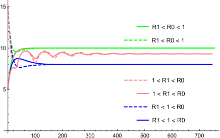
Figure 1: The uninfected cells $X_{n}$ along time.

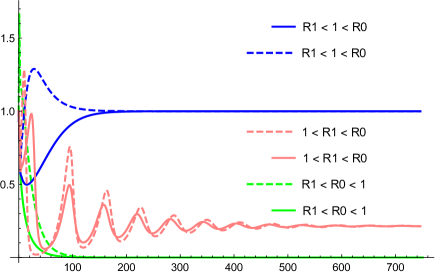
Figure 2: The infected cells $Y_{n}$ along time.

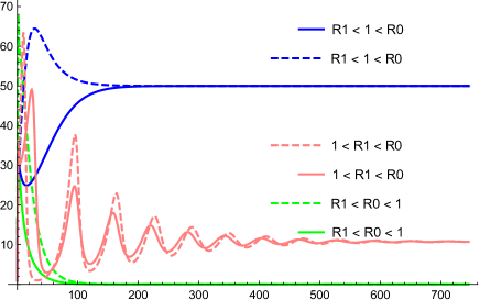
Figure 3: The HIV virus $V_{n}$ along time.

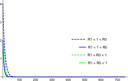
Figure 4: The CTL cells $Z_{n}$ along time (Cases I and II).

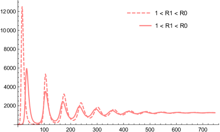
Figure 5: The CTL cells $Z_{n}$ along time (Case III).

In Figures 1, 2 and 3, it is represented the behavior $X_{n}$, $Y_{n}$ and $V_{n}$ for Cases I, II, and III. In Figure 4, it is represented Cases I and II, while in Figure 5 it is represented the Case III, for better representation of the behavior $Z_{n}$ of the CTL cells.

4 Conclusion

In this work, we have proposed and studied the global stability of a delayed discrete-time HIV viral infection model with CTL immune response. The model describes the interaction between uninfected cells, infected cells, HIV free viruses, and CTL immune response, analogous to the continuous model investigated in [1]. In the discrete case it was incorporated an intracellular time delay. For this model we prove the existence of positive and bounded solutions, showing that the model is well posed. There are two threshold parameters, the basic reproduction number $\mathcal{R}_{0}$ and the immune response activation number $\mathcal{R}_{1}$. We determined the three equilibrium points and related their existence with the previous threshold numbers. Next, using suitable Lyapunov functions and LaSalle’s invariance principle, we proved the global stability for each one of the equilibrium points, extending the results obtained in the continuous model. With the same data used in the literature for the continuous-time model, we made some simulations, which show the consistence between theoretical and numerical results.

References

• [1] Allali, K., Harroudi, S., Torres, D.F.M.: Analysis and optimal control of an intracellular delayed HIV model with CTL immune response. Math Comput. Sci, vol. 12(2), pp. 111–127 (2018) arXiv:1801.10048
• [2] Blattner, W., Gallo, R.C., Temin, H.M.: HIV causes AIDS. Science, vol. 241(4865), pp. 515–516 (1988)
• [3] Busch, M.P., Satten, G.A.: Time course of viremia and antibody seroconversion following human immunodeficiency virus exposure. Am. J. Med, vol. 102(5B), pp. 117–126 (1997)
• [4] Ciupe, M.S., Bivort, B.L., Bortz, D.M., Nelson, P.W.: Estimating kinetic parameters from HIV primary infection data through the eyes of three different mathematical models. Math. Biosci., vol. 200(1), pp. 1–27 (2006)
• [5] Culshaw, R., Ruan, S., Spiteri, R.J.: Optimal HIV treatment by maximizing immune response. J. Math. Biol., vol. 48(5), pp. 545–562 (2004)
• [6] DeBoer, R.J., Perelson, A.S.: Target cell limited and immune control models of HIV infection: a comparison. J. Theor. Biol., vol. 190(3), pp. 201–214 (1998)
• [7] Elaiw, A. M., Alshaikh, M. A.: Global stability of discrete virus dynamics models with humoural immunity and latency. J. Biol. Dyn., vol. 13(1), pp. 639–674 (2019)
• [8] Elaydi, S.: An introduction to difference equations, 3rd ed. Springer, New York (2005)
• [9] Kahn, J.O., Walker, B.D.: Acute human immunodeficiency virus type 1 infection. N. Engl. J. Med., vol. 339(1), pp. 33–39 (1998)
• [10] Kirschner, D.: Using mathematics to understand HIV immune dynamics. Not. Am. Math. Soc., vol. 43(2), pp. 191–202 (1996)
• [11] Mickens, R.E.: Nonstandard finite difference models of differential equations. World Scientific Publishing Co., Inc., River Edge, NJ (1994)
• [12] Mickens, R.E.: Nonstandard finite difference schemes for differential equations. J. Difference Equ. Appl., vol. 8(9), pp. 823–847 (2002)
• [13] Mickens, R.E.: Dynamic consistency: a fundamental principle for constructing nonstandard finite difference schemes for differential equations. J. Difference Equ. Appl., vol. 11(7), pp. 645–653 (2005)
• [14] Mickens, R.E.: Calculation of denominator functions for nonstandard finite difference schemes for differential equations satisfying a positivity condition. Numer. Methods Partial Differential Equations, vol. 23, pp. 672–691 (2007)
• [15] Nowak, M., May, R.: Mathematical biology of HIV infection: antigenic variation and diversity threshold. Math. Biosci., vol. 106(1), pp. 1–21 (1991)
• [16] Pawelek, K.A., Liu, S., Pahlevani, F., Rong, L.: A model of HIV-1 infection with two time delays: mathematical analysis and comparison with patient data. Math. Biosci., vol. 235(1), pp. 98–109 (2012)
• [17] Perelson, A.S., Nelson, P.W.: Mathematical analysis of HIV-1 dynamics in vivo. SIAM Rev., vol. 41(1), pp. 3–44 (1999)
• [18] Perelson, A.S., Neumann, A.U., Markowitz, M., Leonard, J.M., Ho, D.D.: HIV-1 dynamics in vivo: virion clearance rate, infected cell life-span, and viral generation time. Science, vol. 271(5255), pp. 1582–1586 (1996)
• [19] Rocha, D., Silva, C.J., Torres, D.F.M.: Stability and optimal control of a delayed HIV model. Math. Methods Appl. Sci., vol. 41(6), pp. 2251–2260 (2018) arXiv:1609.07654
• [20] Shi, P., Dong, L.: Dynamical behaviors of a discrete HIV-1 virus model with bilinear infective rate. Math Methods Appl. Sci., vol. 37(15), pp. 2271–2280 (2014)
• [21] Silva, C.J., Torres, D.F.M.: A TB-HIV/AIDS coinfection model and optimal control treatment. Discrete Contin. Dyn. Syst., vol. 35(9), pp. 4639–4663 (2015) arXiv:1501.03322
• [22] Silva, C.J., Torres, D.F.M.: A SICA compartmental model in epidemiology with application to HIV/AIDS in Cape Verde. Ecological Complexity, vol. 30, pp. 70–75 (2017) arXiv:1612.00732
• [23] Stafford, M.A., Corey, L., Cao,Y., Daar, E.S., Ho, D.D., Perelson, A.S.: Modeling plasma virus concentration during primary HIV infection. J. Theor. Biol., vol. 203(3), pp. 285–301 (2000)
• [24] Vaz, S., Torres, D.F.M.: A dynamically-consistent nonstandard finite difference scheme for the SICA model. Math. Biosci. Eng., vol. 18(4), pp. 4552–4571 (2021) arXiv:2105.10826
• [25] Weiss, R.: How does HIV cause AIDS? Science, vol. 260(5112), pp. 1273–1279 (1993)