On the physical size of the Milky Way globular cluster NGC 7089 (M 2)

Abstract

We study the outer regions of the Milky Way globular cluster NGC 7089 based on new Dark Energy Camera (DECam) observations. The resulting background cleaned stellar density profile reveals the existence of an extended envelope. We confirm previous results that cluster stars are found out to $\sim$ 1$\degr$ from the cluster’s centre, which is nearly three times the value of the most robust tidal radii estimations. We also used results from direct $N$-body simulations in order to compare with the observations. We found a fairly good agreement between the observed and numerically generated stellar density profiles. Because of the existence of gaps and substructures along globular cluster tidal tails, we closely examined the structure of the outer cluster region beyond the Jacobi radius. We extended the analysis to a sample of 35 globular clusters, 20 of them with observed tidal tails. We found that if the stellar density profile follows a power law $\propto$ $r^{-\alpha}$, the $\alpha$ slope correlates with the globular cluster present mass, in the sense that, the more massive the globular cluster the smaller the $\alpha$ value. This trend is not found in globular clusters without observed tidal tails. The origin of such a phenomenon could be related, among other reasons, to the proposed so-called potential escapers or to the formation of globular clusters within dark matter mini-haloes.

1 Introduction

The detection of tidal tails in Milky Way globular clusters is relevant in the context of the globular cluster formation environment. Some recent results suggest that the absence of tidal tails is related to the fact that globular clusters formed within dark matter mini-halos, and role reversal (Starkman et al., 2019; Boldrini & Vitral, 2021; Wan et al., 2021). According to Boldrini et al. (2020) halo globular clusters formed at or near the centre of small dark matter halos still retain to the present day an excess of dark matter above the galactic background dark matter. Carlberg & Grillmair (2021) searched for signatures of dark matter mini-halos in a sample of 25 Milky Way globular clusters. When the globular cluster sample is matched with the compilation of globular clusters with studies of their outer structures by Piatti & Carballo-Bello (2020, see their Table 1), we found that several globular clusters without tidal tails do not show rising velocity dispersion profiles, as expected for those embedded in dark matter mini-halos (Bonaca et al., 2019). What we mention above explains in some way why the study of the outermost regions of globular clusters, searching for any kind of extra-tidal feature, is nowadays an active field of research.

In this work we focus on NGC 7089 (M 2), a globular cluster whose stellar structure has previously been analyzed from different data-sets and methodologies, and for which different results have been obtained. Grillmair et al. (1995) studied the outer structure of 12 Milky Way globular clusters, among them, NGC 7089. They used photographic photometry, and concluded that the spatial distribution of stars with magnitudes and colours consistent with the cluster main sequence shows the appearance of tidal tails in their two-dimensional surface density map. Although these extra-tidal stars limited the accuracy of the cluster tidal radius, they determined a King (1966)’s model tidal radius of 15.9$\arcmin$. Later, Dalessandro et al. (2009) used HST data to trace the cluster surface density profile and to fit a King model, and obtained a smaller tidal radius of 9.2$\arcmin$. Jordi & Grebel (2010) also investigated 17 Milky Way globular clusters to identify tidal tails emerging from them. They employed the Sloan Digital Sky Survey (SDSS) Data Release 7 (Abazajian et al., 2009). The density contours generated from a colour-magnitude weighted algorithm to map potential cluster members resulted similar to the background contours. Contrarily to the expected possible inner tidal tails aligned with the orbital path of the cluster no large scale features were detected. Jordi & Grebel (2010) derived a mean cluster tidal radius of 11.7$\arcmin$, 25$\%$ smaller than that of Grillmair et al. (1995).

NGC 7089 was also targeted for a search of stellar streams in the outer Galactic halo by Kuzma et al. (2016), who studied its surroundings from Dark Energy Camera and MegaCam data sets. They selected it on the basis of a variety of unusual characteristics, which appeared suggestive of an extra-Galactic origin. Indeed, the cluster stellar population exhibits a broad dispersion in Fe and neutron capture elements. The authors concluded that NGC 7089 might plausibly constitute the stripped nucleus of a dwarf galaxy that was accreted and destroyed by the Milky Way in the past, although they could not identify the origin of an extended diffuse stellar envelope, which embeds it. Such stellar envelope reaches at least $\sim$ 60$\arcmin$, i.e., several times the tidal radii mentioned above, and has a nearly circular shape, which decreases in stellar density following a power law with slope $\alpha$ = -2.2$\pm$0.2.

More recently, de Boer et al. (2019) used Gaia DR2 data (Gaia Collaboration et al., 2016, 2018) to build radial number density profiles of 81 Milky Way globular clusters. Unlike previous studies, they performed a cluster membership selection from proper motions rather than from magnitudes and colours. de Boer et al. (2019) fitted the density profiles using a set of single-mass models, among them King’s (King, 1966) and Wilson’s (Wilson, 1975) models, generalized lowered isothermal models, and a spherical potential escapers stitched (SPES) model. For NGC 7089, the model that best resembles the cluster density profile is the SPES one, with an associated tidal radius of 19.2$\arcmin$. As can be suspected, the larger tidal radius could be reflecting the existence of an extended envelope or tidal tails. We note that Sollima (2020) using the same Gaia DR2 database did not find any tidal tails. However, long tidal tails associated to NGC 7089 have been recently detected by Ibata et al. (2021), who employed Gaia EDR3 data and the streamfinder algorithm (Malhan & Ibata, 2018), and by Grillmair (2022).

In the merger history of the Milky Way, NGC 7089 is associated to the Gaia-Enceladus dwarf galaxy with other 12 globular clusters (Kruijssen et al., 2020). Among them, 7 have been targeted by studies of their outer regions seeking for hints of tidal tails, namely: NGC 4147 and NGC 6205 (Jordi & Grebel, 2010), NGC 6341 (Sollima, 2020), NGC 6779 (Piatti & Carballo-Bello, 2019), NGC 6864 (Piatti, 2022), NGC 7099 (Piatti et al., 2020), and NGC 7492 (Navarrete et al., 2017). Only NGC 4147 and 7492 exhibit tidal tails. We might infer from these results that most Gaia-Enceladus globular clusters do not have tidal tails, but they do not have rising velocity dispersions at large radii as they could have formed within dark matter mini-halos (Carlberg & Grillmair, 2021), which would challenge theoretical models of the formation of globular clusters (Peebles, 1984; Searle & Zinn, 1978).

Precisely, Carballo-Bello et al. (see Section 2) embarked in an observing campaign of Gaia-Enceladus globular clusters with the aim of increasing the number of member clusters with detailed studies of their outer regions, in order to classify them as clusters with tidal tails, or with extra-tidal envelopes, or without detectable signatures of extra-tidal structures (NGC 6809 (Piatti, 2021); NGC 6864 (Piatti, 2022); NGC 6981 (Piatti et al., 2021); NGC 7099 (Piatti et al., 2020)). We focus here on NGC 7089, the last cluster in Carballo-Bello et al.’s sample. A complete census of the outer regions of Gaia-Enceladus globular clusters will shed light onto our understanding of whether the formation conditions prevail over times, or the orbital history in the Milky Way prevails.

In Section 2 we describe the data sets used, while in Section 3 we use this data to build the stellar number density profile of NGC 7089. Section 4 deals with the computation of the cluster orbit from $N$-body simulations, whose results are compared with those from the observational data and discussed in Section 5. Although NGC 7089 has been studied extensively, this work contributes to our knowledge of its outer stellar structure from the focused analysis on a cluster colour-magnitude diagram in the SDSS $g$ and $i$ filters, cleaned from field star contamination using an independent procedure, and from numerical simulations, which are performed for the first time. We note that previous works derived tidal radii spanning from 9.2$\arcmin$ up to 19.2$\arcmin$, revealing a real challenge in estimating the cluster’s extension.

2 Photometric data set

To explore the outskirts of NGC 7089, we used images obtained with the Dark Energy Camera (DECam), which is attached to the prime focus of the 4-m Blanco telescope at Cerro Tololo Inter-American Observatory (CTIO). DECam is an array of 62 identical chips with a scale of 0.263 arcsec pixel^-1 that provides a 3 deg² field of view (Flaugher et al., 2015). The images were taken as part of the observing program CTIO 2019B-1003 (PI: Carballo-Bello) and are now of public access. NGC 7089 and a comparison field located 5$\degr$ eastward were imaged with 4$\times$600 sec $g$ and 4$\times$400 sec $r$ exposures, respectively, under photometric conditions. Additionally, observations of 5 SDSS fields at different airmass are also available, which were used to derive the atmospheric extinction coefficients and the transformations between the instrumental magnitudes and the SDSS $ugriz$ system (Fukugita et al., 1996).

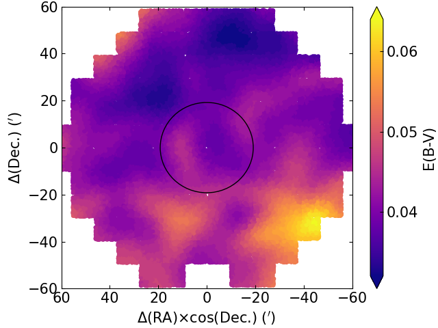
Figure 1: Reddening variation across the field of NGC 7089. The black circle corresponds to the cluster SPES tidal radius (19.2$\arcmin$) derived by de Boer et al. (2019).

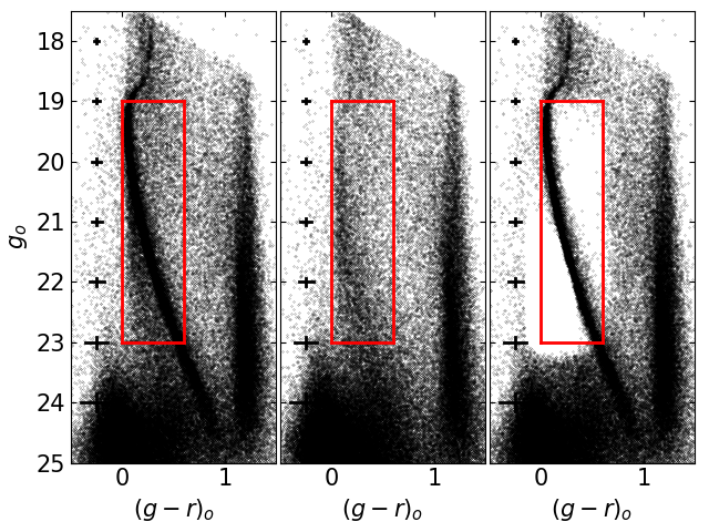
Figure 2: Intrinsic CMDs for all the measured stars in the cluster field (left panel) and in the comparison field (middle panel). The cleaned cluster CMD (only for the red delimited region) is shown in the right panel. Typical error bars are also indicated.

The images were processed following the DECam Community Pipeline (Valdes et al., 2014), and the resulting processed images were employed to obtain the corresponding photometry using the daophot ii/allstar point-spread-function fitting routines (Stetson et al., 1990). Since bad pixels, unresolved double stars, cosmic rays, and background galaxies contaminate our resulting photometric catalogs, we avoided their presence in our subsequent analysis by imposing the restriction of keeping positions and standardized $g$ and $r$ magnitudes of objects with $|$sharpness$|$ $\leq$ 0.5. Finally, the photometry completeness was estimated from artificial star tests, using the daophot ii routines and the same quality selections as for observations, as follows: synthetic stars were added with magnitudes and positions distributed similarly to those of the measured stars in each image; their photometry was carried out similarly as described above; and the resulting magnitudes for the synthetic stars were compared with those used to create such stars. While performing the artificial star tests, we treated each image without distinguishing between inner and outer cluster regions. Therefore, on average, the 50$\%$ completeness level resulted to be 23.4 mag and 23.3 mag for the $g$ and $r$ bands, respectively. We used these magnitudes as a reference while choosing the colour-magnitude diagram regions for building the cluster number density profile.

Fig. 1 shows that there is no evidence of differential reddening in the NGC 7089 field, with $E(B-V)$ values retrieved from the NASA/IPAC Infrared Science Archive using an input uniform grid of Right Ascension and Declination values covering the entire DECam field of view in steps of 1 arcmin, respectively. The resulting range of reddening values ($\Delta$$E(B-V)$ = 0.035 mag) is clearly small. We corrected the observed $g$ and $r$ magnitudes of each star by using the $E(B-V)$ colour excesses according to the positions of the stars in the sky. For the same of the reader, we computed a mean $E(B-V)$ value for the comparison field of 0.10$\pm$0.02 mag.

We started our analysis by inspecting the cluster colour-magnitude diagram (CMD) shown in the left panel of Fig. 2, which includes all measured stars. As can be seen, Fig. 2 shows the long cluster main sequence and the peculiar contribution of the Milky Way composite star field population, which can be recognized from the comparison with the star field CMD (middle panel of Fig. 2) built from all measured stars in a DECam field located 5$\degr$ to the East of the cluster’s centre.

3 Stellar number density profile

A standard approach to build stellar radial profile was used by Carballo-Bello et al. (2014) (see, e.g., Olszewski et al., 2009; Saha et al., 2010; Roderick et al., 2015; Kuzma et al., 2016; Kuzma et al., 2018). However, they did not get rid of field stars that populate the cluster main sequence too. de Boer et al. (2019) employed stars down to Gaia $G$ = 20 mag with proper motions similar to the mean cluster proper motion. We note that main sequence stars are far more numerous than red giants, so that they are better tracers of low cluster star densities. We here decided to use main sequences stars, because stars with smaller masses can be found more easily far away from the cluster main body (Carballo-Bello et al., 2012). For this reason, most of the studies devoted to the search for extra-tidal structures have used relatively faint main sequence stars (see, e.g., Olszewski et al., 2009; Saha et al., 2010). We also cleaned the cluster main sequence from field star contamination, so that the distribution in the sky of the stars that remained unsubtracted represents the intrinsic spatial distribution of cluster members. We describe the process to perform the CMD cleaning in the subsequent text.

Figure 2 shows a region on the cluster main sequence enclosed within red boundaries. We selected that portion of the cluster main sequence to build the respective stellar number density profile, once it is cleaned from field star contamination. The route of this cleaning procedure starts by superimposing the comparison field CMD on to the cluster CMD; then subtracting from the latter as many stars are in the comparison field CMD, choosing those with magnitudes and colours as similar as those of the comparison field stars. The method employed was introduced by Piatti & Bica (2012), which was satisfactorily applied elsewhere (e.g., Piatti et al., 2018; Piatti, 2022, and references therein). The field star decontamination technique proved to be successful for clusters projected on to crowded fields and affected by differential reddening (see, e.g., Piatti & Fernández-Trincado, 2020, and references therein). In order to clean the selected cluster main sequence region, the method uses the CMD of the comparison star field as reference and subtracts from the cluster CMD the closest star in the magnitude versus colour plane to each field star. It assumes that both CMDs share similar field star properties, namely, magnitude and colour distributions, and stellar density.

The strategy to choose stars to subtract from the selected cluster CMD region with magnitudes and colours similars those of the stars in the comparison field CMD consists in defining boxes centred on the magnitude and colour of each star of the comparison star field; then to superimpose them on the cluster CMD, and finally to choose one star per box to subtract. Ideally, stars with the same magnitudes and colours of the comparison field stars are desirable. Because this requirement is difficult to accomplish, stars with magnitudes and colours as close to those of the comparison field stars are chosen. On the other hand, because of stochastic effects of field stars, it could not be straightforward to find a star to subtract in the cluster CMD close to certain (magnitude,colour) pair, corresponding to the magnitude and colour of a field star. In order to assure the subtraction of one star in the cluster CMD per field star in the comparison field CMD, we started by searching reasonable large areas in the cluster CMD around the (magnitude,colour) values of each field star. We started with boxes with size of ($\Delta$$g_{0}$,$\Delta$$(g-r)_{0}$) = (0.25 mag, 0.10 mag) centred on the ($g_{0}$, $(g-r)_{0}$) values of each comparison field star, in order to guarantee to find a star in the cluster CMD with the magnitude and colour within the box boundary. In the case that more than one star is located inside that box, the closest one to the centre of that (magnitude, colour) box is subtracted. Because magnitudes and colours of stars in the cluster CMD have uncertainties, the number of stars that fall inside the boundary of a (magnitude,colour) box depends on whether we consider them. For this reason, the magnitude and colour errors of the stars in the cluster CMD were taken into account while searching for a star to subtract. With that purpose, we allowed the stars in the cluster CMD to vary their positions within an interval of $\pm$1$\sigma$, where $\sigma$ represents the errors in their magnitude and colour, respectively. We allowed up to a thousand random combinations of their magnitude and colour errors. Note that the size of the (magnitude,colour) box where the search of a star similar in magnitude and colour to a field star is carried out is not delimited by the magnitude and colour uncertainties of the stars in the cluster CMD. They are all of the initial size mentioned above, and inside them the search for the closest star to its centre is performed.

The aim of the cluster CMD cleaning procedure is to eliminate from it fields stars, so that only the intrinsic cluster CMD features are visible; the position in the sky of the stars is not relevant, provided that all of them are within the cluster main body. However, when extra-tidal structures or tidal tails are searched and large areas reaching far from the cluster centre are analyzed, the positions in the sky of the subtracted stars play a role. The results are different if the subtracted stars are all distributed inside that cluster main body or throughout a larger area. Precisely, the observation of a comparison field located far from the cluster is aimed at cleaning a reasonable large area around the cluster main body. Because of the relatively large extension of the cleaned cluster area ($\sim$2$\degr$$\times$2$\degr$; see Fig. 1), we imposed the condition that the spatial positions of the stars to subtract from the cluster CMD were chosen randomly. Thus, we avoided spurious overdensities in the resulting cleaned cluster area driven by the subtraction of stars from the cluster CMD that are located nearly in the same sky regions. In practice, for each comparison field star, we first randomly selected the position of a box of 0.05$\degr$ a side in the cluster field (see Fig. 1) where to subtract a star. We then looked for a star with ($g_{0}$, $(g-r)_{0}$) values within the (magnitude, colour) box defined as described above, taking into account the photometric errors. If no star is found in the selected spatial box, we repeated the selection a thousand times, otherwise we enlarged the box size in steps of 0.01$\degr$ a side, to iterate the process. This alternative is useful when the number of remaining not subtracted stars with a desire magnitude and colour is very small, and a star with such magnitude and colour should be find to subtract. In practice, stars that meet the required magnitude and colour selection are mostly find inside the initial 0.05$\degr$$\times$5$\degr$ boxes randomly distributed across the DECam field. Note that the CMD cleaning technique for large areas deals with two main searches, namely; that of stars in the cluster CMD with magnitudes and colours similar to those of field stars, and the positions in the sky of those subtracted stars. Both iterative searches can be carried out indistinctly of the order of the seach.

The outcome of the cleaning procedure is a cluster CMD decontaminated from field stars, i.e., it likely contains only cluster members; their spatial distribution relies on a random selection basis. The number of subtracted stars is equal to that in the comparison star field, because the subtraction is performed in a star-by-star basis. However, it could happen that inside a CMD box there is no star to subtract and in this case the total number of subtracted stars is smaller than that in the comparison field CMD. This can be checked by counting the number of stars in both the comparison field CMD and those subtracted from the cluster CMD. In our case, we subtracted the same number of stars. Fig. 2 (right panel) shows the resulting cluster CMD with the delimited rectangular region decontaminated from field stars. By comparing the observed cluster CMD (left panel) with that of the comparison star field (middle panel), it is readably visible that most of the field star contamination has been eliminated in the cleaned cluster CMD. The cleaned cluster main sequence exhibits the expected shape, with a well-defined lower envelope and a blurred upper one caused by the presence of binary stars. Some isolated stars are visible in the upper-right corner of the devised rectangle, which can possible come from intrinsic differences between the comparison star field population and that projected along the line-of-sight of the cluster. NGC 7089 and comparison field Galactic coordinates are (l,b) = (53.4$\degr$,-35.8$\degr$) and (56.9$\degr$,-39.8$\degr$), respectively. They do not affect the analysis of the outermost regions of NGC 7089. On the contrary, the cleaned CMD regions beyond the cluster main sequence validate the subtraction procedure. The cleaned CMD also shows that beyond the cleaned region (the red rectangle), toward bluer and fainter magnitudes, some stars were subtracted. This is because we considered the uncertainties in magnitude and colour, so that for a box placed in the bottom-left corner of the CMD region, stars outside it were selected. The subtraction of these stars have no effects in our analysis. The most important CMD region to clean is that along the cluster main sequence, because we use cluster members to build the cluster density profile. We executed 1000 times the decontamination procedure, and defined a membership probability $P$ ($\%$) as the ratio $N$/10, where $N$ is the number of times a star was found among the 1000 different outputs. In the subsequence analysis we only kept stars with $P$ $>$ 70$\%$.

We used stars in the cleaned cluster CMD rectangular region to build the respective stellar radial profile. In order to do that, we counted the number of stars in annuli of 1.2$\arcmin$, 2.4$\arcmin$, 3.6$\arcmin$, 4.8$\arcmin$ and 6.0$\arcmin$ wide, and computed their average and dispersion. The resulting radial profile with its respective uncertainties is depicted in Fig. 3, where we included the SPES model fitted by de Boer et al. (2019). For comparison purposes, we normalized it to the same density at $r$=6.6$\arcmin$. As can be seen, the present stellar radial profile extend beyond the SPES tidal radius, which is the largest value that we found in the literature (see Section 1). The radial profile built by Kuzma et al. (2016, their figure 8) (grey diamonds in Fig. 3) confirms that there is an excess of stars distributed beyond the SPES tidal radius. Note that the shapes of both radial profiles are remarkably similar.

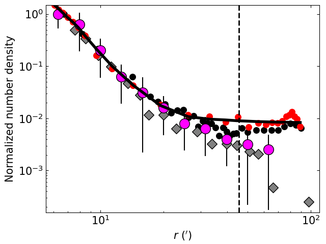
Figure 3: Resulting number density profile for stars in the field star decontaminated cluster CMD region. represented with filled magenta circles. Error bars are also drawn. The black solid curve is the SPES model fitted by de Boer et al. (2019). Grey diamonds represent the stellar radial profile obtained by Kuzma et al. (2016); red filled circles that by de Boer et al. (2019), while black filled circles are obtained from the $N$-body experiment. The vertical dashed line is the cluster Jacobi’s radius (45.5$\arcmin$, de Boer et al., 2019).

3.1 $N$-body simulations

We also ran a number of direct $N$-body simulations of NGC 7089 in order to compare the observed density profile with the theoretically expected one for a cluster that has the same mass and is on the same orbit as NGC 7089. In order to perform the $N$-body simulations, we used the NBODY+P3T code from Arnold et al. (2021). This code treats gravitational interactions between stars in close proximity to each other with a fourth order Hermite integration scheme and calculates distant gravitational forces using Bonsai (Bedorf & Portegies Zwart, 2020), a Barnes-Hut tree code with a standard leap frog scheme. In order to achieve a better performance, we modified the integration routine to use a single leap frog scheme, with all gravitational forces calculated using the Tree code. We chose a critical opening angle of $\theta=0.4$, a leapfrog integration step size of $\Delta t=\frac{1}{32}$ and a softening length of $\epsilon=0.03$ in $N$-body units (corresponding to about 0.1 pc in physical units or about 1/10th of the core size of NGC 7089) as the best trade-off between accuracy and speed. This way we were able to perform single simulation of NGC 7089, which would normally take several months with a direct $N$-body code like NBODY6, in less than two days.

The general set-up of our simulations follows the ones done in Wan et al. (2021). We integrated a point-mass particle backwards in time along the orbit of NGC 7089 for 2 Gyr with a 4th order Runge-Kutta integrator, using the Milky Way potential by Irrgang et al. (2013). We then set up a star-by-star model of NGC 7089 using the best-fitting model from the grid of $N$-body simulations by Baumgardt (2017) and Baumgardt & Hilker (2018). This model was then integrated forward in time for 2 Gyr to the present-day position of NGC 7089 using NBODY+P3T. We slightly varied the mass and size of the initial $N$-body model until we achieved the best-match of our model cluster to the observed NGC 7089.

We then used the result of the best-fitting $N$-body simulation to construct a stellar density proifile, similarly to that of Fig. 3. We then selected from the $N$-body simulation results stars within those mass regimes distributed throughout a region of 2$\degr$$\times$2$\degr$ centred on the cluster as in Fig. 2, and built the respective stellar density profile by applying the same recipe as above. The resulting stellar number density profile is depicted in Fig. 3 with black filled circles . As can be seen, there is a clear excess beyond the SPES radius, in very good agreement with the present one and that obtained by Kuzma et al. (2016).

4 Analysis and discussion

As far as we are aware, this is the first time that the result of the detailed outer structure of NGC 7089 built by Kuzma et al. (2016) is confirmed. We used both, independent data sets and $N$-body simulations to show that NGC 7089 has an extended envelope beyond the largest tidal radius derived up-to-date. Furthermore, we think that the wide range of previous tidal radius estimates (from 9.2$\arcmin$ up to 19.2$\arcmin$) is the result of a combination of a low stellar density structure and the use of data reaching different magnitude limits. Sollima (2020) used Gaia DR2 data sets to explore 5$\degr$ in radius around NGC 7089. He restricted the search for extra-tidal features to stars brighter than $G$ = 21 mag and applied a 5D mixture modeling technique and did not find any hints for tidal tails. With DECam and MegaCam images Kuzma et al. (2016) went even deeper, gaining $\sim$ 2.5 mag in the limiting magnitude. This means that they could compare the radial profile of mainly read giant stars derived from Gaia data with that built from much less massive stars. They did not find tidal tails but a low density extended envelope following a power law with slope $\alpha$ =-2.2$\pm$0.2.

The existence of tidal tails requires the exploration of larger areas, since they usually show variations in the stellar density, with the appearance of gaps, spurs, and substructures (Odenkirchen et al., 2001; Grillmair & Dionatos, 2006; Carlberg et al., 2012; Erkal et al., 2017; de Boer et al., 2020). Indeed, the long tidal tails of NGC 7089 identified by Ibata et al. (2021) and Grillmair (2022) show variations of their stellar densities. Its leading and trailing tidal tails turned out to be asymmetric. Both tails are nearly aligned along the direction toward the Milky Way centre. We note that the cluster’s orbit has an eccentricity of 0.94 and an inclination angle of 84.18$\degr$, so that it describes a trajectory which pass very close to the Milky Way centre (perigalacticon ($R_{peri}$) = 0.84$\pm$0.06 kpc, apogalacticon ($R_{apo}$) = 18.80$\pm$0.29 kpc) (Baumgardt et al., 2019), which explains the tidal tails orientation (Montuori et al., 2007). At the present time, NGC 7089 is nearly midway between its perigalacticon and apogalacticon (($R_{apo}$ - $R_{GC}$)/$R_{apo}$ = 0.45) at a galactocentric distance of $R_{GC}$ = 9.68 kpc. Piatti et al. (2019) estimated the ratio of the cluster mass lost by tidal disruption to the total cluster mass for Milky Way globular clusters ($M_{disp}/M_{ini}$), and derived a value of 0.29 for NGC 7089. This value is similar to that of Pal 5 (0.24), which exhibits a $\sim$ 30$\degr$ long tidal tail (Starkman et al., 2019) and its orbit is also inclined (65.13$\degr$) (Baumgardt et al., 2019). However, the latter does not reach the Milky Way bulge ($R_{peri}$ = 17.40 kpc) as NGC 7089 does, and its orbit is not elongated as the NGC 7089’s orbit (Pal 5 orbit’s eccentricity=0.17). These similarity and difference could help in disentangling the origin of tidal tails in globular clusters, and their shapes and substructures, to the light of two main scenarios, namely, the structure of the Milky Way (e.g., giant molecular clouds, the bar, spiral arms), or the presence of a population of dark matter subhalos. At this point, it is worth mentioning that Zhang & Mackey (2021) showed for a sample of nine Milky Way halo globular clusters that the presence of tidal tails is subjected to the particular cluster dynamical history.

Bearing in mind that tidal tails does not necessarily emerge from the globular cluster main body as a steady, smooth stellar density distribution, we focused on the analysis of the extra-tidal features composed by stars that have escaped the cluster, i.e., those that are placed at distances to the globular cluster’s centre larger than its Jacobi radius. We seek any hint for a difference between globular clusters that exhibit tidal tails with respect to those without them. For that purpose, we used the recent compilation by Zhang & Mackey (2021, see their Table 3) of Milky Way globular clusters with studies of their outermost regions. They split the globular clusters into three groups, namely: globular clusters with tidal tails (T); those with extended envelopes (E), and clusters without any signature of extra-tidal features (N). We explored homogeneously the outer regions of these globular clusters by using the stellar number density profiles built by de Boer et al. (2019) using Gaia DR2 data, and their adopted globular clusters’ Jacobi radii. We found 36 globular clusters in common between de Boer et al. (2019) and Zhang & Mackey (2021), and excluded NGC 5904 from the fit because there is no data outside its Jacobi radius. Fig. 3 illustrates the Jacobi radius of NGC 7089 with a vertical dashed line and its Gaia DR2 stellar density profile depicted with filled red circles, respectively.

We fitted their stellar number density profiles with a power law $\propto$ $r^{-\alpha}$ using points placed farther than the globular clusters’ Jacobi radii. The resulting $\alpha$ slopes are listed in Table 1, as well as the number of points ($N$) used during the fit, and the groups to which the globular clusters belong (T=with tidal tails; E=with extended envelop; N=without extra-tidal signature). As can be seen, the resulting $\alpha$ slopes are smaller than 1.0, with the sole exception of that for Pal 1 (1.52). The value obtained for NGC 7089 (-0.65) differs from that of Kuzma et al. (2016, 2.2), because the latter considered a much inner region -inside the Jacobi radius-, where a decreasing stellar number density is apparent (see Fig. 3). We also note that the $N$-body stellar density profile agrees well with that built by de Boer et al. (2019) for the whole distance range used. This is not the case of the stellar number density profiles derived here and by Kuzma et al. (2016), possibly because of the lack of a better statistics at the boundaries of the observed fields.

We tried to correlate these $\alpha$ slopes with different astrophysical properties (e.g., Galactocentric distance, orbital parameters, structural properties, relaxation times), and found that it shows a trend with the present cluster mass (Baumgardt et al., 2019) for globular cluster with tidal tails. Fig. 4 shows the suggestive correlation, where the symbol size is proportional to the number of points $N$ used to derive the $\alpha$ values, and the red line represents a linear least-square fit. As can be seen, the larger the globular cluster mass, the smaller the $\alpha$ slope; a trend that is not observed in globular clusters with only extended envelopes or without any extra-tidal feature. These findings suggests that most massive globular clusters with observed tidal tails can exhibit increasing stellar overdensites beyond their Jacobi radii, while their less massive counterparts show decreasing stellar overdensities as a function of the distance to the globular cluster centre. We also note that no points should have been registered beyond the Jacobi radii of globular clusters without extra-tidal features. However, the registered extensions of globular clusters recovered by de Boer et al. (2019) from Gaia DR2 data could differ from the Jacobi radii used, which were determined by Balbinot & Gieles (2018), or else, the group to which a globular cluster was included could be different. Nevertheless, if the entire globular cluster sample were treated as having tidal tails, the trend observed for those grouped in the T group would remain with a larger scatter.

Piatti & Carballo-Bello (2020) and Zhang & Mackey (2021) searched for overall kinematic or structural conditions that have allowed some Milky Way globular clusters to develop tidal tails, and found that globular clusters behave similarly irrespective of the presence of tidal tails or any other kind of extra-tidal feature, or the absence thereof. As far as we are aware, the present outcome is the first observed distinction between globular clusters in the T and E and N groups. Some hints to explain the correlation between the $\alpha$ slope for distances larger than the Jacobi radius and the globular cluster mass (top panel of Fig. 4) could be found in the proposed so-called potential escapers, which would give rise of the stellar of the density and velocity dispersion near the Jacobi radius (Baumgardt, 2001; Küpper et al., 2010; Claydon et al., 2019). Such a rising velocity dispersion at large radii was also suggested by Carlberg & Grillmair (2021) as an observing feature for globular clusters that could have formed within dark matter mini-halos.

Table 1: Power law slopes ($\alpha$) of Gaia DR2 stellar density profiles of Milky Way globulars for distances beyond their Jacobi radii. The number of points used in the fits ($N$) and the globular cluster class according to Zhang & Mackey (2021, T= with tidal tails; E= with extended envelop; N=without extra-tidal signature) are also listed.

Cluster	$\alpha$	$N$	Group	Cluster	$\alpha$	$N$	Group	Cluster	$\alpha$	$N$	Group
NGC 288	0.10	2	T	NGC 5139	-0.26$\pm$0.04	35	T	NGC 6752	-0.16$\pm$0.15	8	N
NGC 362	-0.28$\pm$0.15	24	T	NGC 5272	-0.49$\pm$0.93	3	T	NGC 6809	0.04$\pm$0.14	13	N
NGC 1261	-0.08$\pm$0.48	9	T	NGC 5466	0.34	2	T	NGC 6864	0.19$\pm$0.38	16	N
NGC 1851	0.22$\pm$0.30	11	T	NGC 5694	0.01$\pm$0.14	134	E	NGC 6981	-0.34$\pm$0.31	14	E
NGC 1904	-0.02$\pm$0.43	12	E	NGC 5824	0.24$\pm$0.14	100	T	NGC 7006	-0.24$\pm$0.15	161	N
NGC 2298	0.54$\pm$0.48	5	T	NGC 5897	0.63$\pm$0.30	11	N	NGC 7078	-0.12$\pm$0.10	34	N
NGC 2419	0.01$\pm$0.30	28	N	NGC 6101	0.43$\pm$0.69	3	T	NGC 7089	-0.65$\pm$0.36	12	T
NGC 2808	0.39$\pm$0.17	23	T	NGC 6205	-0.26$\pm$0.22	7	N	NGC 7099	0.68$\pm$0.29	5	T
NGC 3201	0.23	2	T	NGC 6229	0.07$\pm$0.47	8	N	NGC 7492	-0.83$\pm$0.39	3	N
NGC 4590	0.08	2	T	NGC 6341	0.14$\pm$0.34	6	T	Pal 1	1.52$\pm$0.24	6	T
NGC 5024	-0.28$\pm$0.78	3	T	NGC 6362	0.08$\pm$0.30	5	T	Pal 12	-0.10$\pm$0.93	5	N
NGC 5053	0.33	2	E	NGC 6397	0.99	2	T

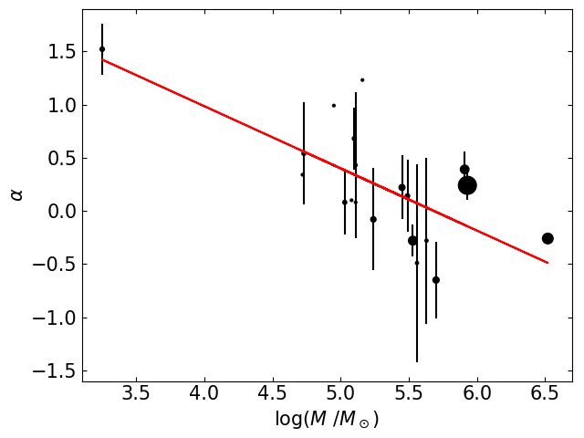
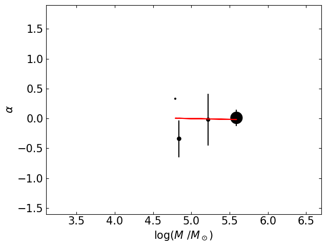
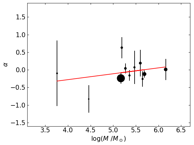
Figure 4: Relationship between the power law $\alpha$ slopes of the outer number density profile (Table 1) and the present globular cluster mass. Top, middle, and bottom panels are for globular clusters in groups T, E, and N, respectively. The size of the filled circles is proportional to the number $N$ in Table 1. The red line represent a linear least-squares fit.

5 Data availability

Data used in this work are available upon request to the first author.

References

- Abazajian et al. (2009) Abazajian K. N., et al., 2009, ApJS, 182, 543
- Arnold et al. (2021) Arnold A. D., Baumgardt H., Wang L., 2021, MNRAS,
- Balbinot & Gieles (2018) Balbinot E., Gieles M., 2018, MNRAS, 474, 2479
- Baumgardt (2001) Baumgardt H., 2001, MNRAS, 325, 1323
- Baumgardt (2017) Baumgardt H., 2017, MNRAS, 464, 2174
- Baumgardt & Hilker (2018) Baumgardt H., Hilker M., 2018, MNRAS, 478, 1520
- Baumgardt et al. (2019) Baumgardt H., Hilker M., Sollima A., Bellini A., 2019, MNRAS, 482, 5138
- Bedorf & Portegies Zwart (2020) Bedorf J., Portegies Zwart S., 2020, SciPost Astronomy, 1, 001
- Boldrini & Vitral (2021) Boldrini P., Vitral E., 2021, arXiv e-prints, p. arXiv:2104.03635
- Boldrini et al. (2020) Boldrini P., Mohayaee R., Silk J., 2020, MNRAS, 492, 3169
- Bonaca et al. (2019) Bonaca A., Hogg D. W., Price-Whelan A. M., Conroy C., 2019, ApJ, 880, 38
- Carballo-Bello et al. (2012) Carballo-Bello J. A., Gieles M., Sollima A., Koposov S., Martínez-Delgado D., Peñarrubia J., 2012, MNRAS, 419, 14
- Carballo-Bello et al. (2014) Carballo-Bello J. A., Sollima A., Martínez-Delgado D., Pila-Díez B., Leaman R., Fliri J., Muñoz R. R., Corral-Santana J. M., 2014, MNRAS, 445, 2971
- Carlberg & Grillmair (2021) Carlberg R. G., Grillmair C. J., 2021, arXiv e-prints, p. arXiv:2106.00751
- Carlberg et al. (2012) Carlberg R. G., Grillmair C. J., Hetherington N., 2012, ApJ, 760, 75
- Claydon et al. (2019) Claydon I., Gieles M., Varri A. L., Heggie D. C., Zocchi A., 2019, MNRAS, 487, 147
- Dalessandro et al. (2009) Dalessandro E., Beccari G., Lanzoni B., Ferraro F. R., Schiavon R., Rood R. T., 2009, ApJS, 182, 509
- de Boer et al. (2019) de Boer T. J. L., Gieles M., Balbinot E., Hénault-Brunet V., Sollima A., Watkins L. L., Claydon I., 2019, MNRAS, 485, 4906
- de Boer et al. (2020) de Boer T. J. L., Erkal D., Gieles M., 2020, MNRAS, 494, 5315
- Erkal et al. (2017) Erkal D., Koposov S. E., Belokurov V., 2017, MNRAS, 470, 60
- Flaugher et al. (2015) Flaugher B., et al., 2015, AJ, 150, 150
- Fukugita et al. (1996) Fukugita M., Ichikawa T., Gunn J. E., Doi M., Shimasaku K., Schneider D. P., 1996, AJ, 111, 1748
- Gaia Collaboration et al. (2016) Gaia Collaboration et al., 2016, A&A, 595, A1
- Gaia Collaboration et al. (2018) Gaia Collaboration et al., 2018, A&A, 616, A1
- Grillmair (2022) Grillmair C. J., 2022, arXiv e-prints, p. arXiv:2203.04425
- Grillmair & Dionatos (2006) Grillmair C. J., Dionatos O., 2006, ApJ, 643, L17
- Grillmair et al. (1995) Grillmair C. J., Freeman K. C., Irwin M., Quinn P. J., 1995, AJ, 109, 2553
- Ibata et al. (2021) Ibata R., et al., 2021, ApJ, 914, 123
- Irrgang et al. (2013) Irrgang A., Wilcox B., Tucker E., Schiefelbein L., 2013, A&A, 549, A137
- Jordi & Grebel (2010) Jordi K., Grebel E. K., 2010, A&A, 522, A71
- King (1962) King I., 1962, AJ, 67, 471
- King (1966) King I. R., 1966, AJ, 71, 276
- Kruijssen et al. (2020) Kruijssen J. M. D., et al., 2020, MNRAS, 498, 2472
- Küpper et al. (2010) Küpper A. H. W., Kroupa P., Baumgardt H., Heggie D. C., 2010, MNRAS, 401, 105
- Kuzma et al. (2016) Kuzma P. B., Da Costa G. S., Mackey A. D., Roderick T. A., 2016, MNRAS, 461, 3639
- Kuzma et al. (2018) Kuzma P. B., Da Costa G. S., Mackey A. D., 2018, MNRAS, 473, 2881
- Malhan & Ibata (2018) Malhan K., Ibata R. A., 2018, MNRAS, 477, 4063
- Montuori et al. (2007) Montuori M., Capuzzo-Dolcetta R., Di Matteo P., Lepinette A., Miocchi P., 2007, ApJ, 659, 1212
- Navarrete et al. (2017) Navarrete C., Belokurov V., Koposov S. E., 2017, ApJ, 841, L23
- Odenkirchen et al. (2001) Odenkirchen M., et al., 2001, ApJ, 548, L165
- Olszewski et al. (2009) Olszewski E. W., Saha A., Knezek P., Subramaniam A., de Boer T., Seitzer P., 2009, AJ, 138, 1570
- Peebles (1984) Peebles P. J. E., 1984, ApJ, 277, 470
- Piatti (2021) Piatti A. E., 2021, MNRAS, 505, 3033
- Piatti (2022) Piatti A. E., 2022, MNRAS, 509, 3709
- Piatti & Bica (2012) Piatti A. E., Bica E., 2012, MNRAS, 425, 3085