First results from the ENTOTO neutron monitor: Quantifying the waiting time distribution

Abstract

We discuss a newly established neutron monitor station installed at the ENTOTO Observatory Research Center outside of Addis Ababa, Ethiopia. This is a version of a mini-neutron monitor, recently upgraded to detect individual neutrons and able to calculate the waiting time distribution between neutron pulses down to $\sim 1$ $\mu$s. From the waiting time distribution we define and calculate a new quantity, the correlation ratio, as the ratio of correlated to uncorrelated neutrons measured inside the monitor. We propose that this quantity can, in future, be used as a proxy for spectral index of atmospheric particles incident on the monitor and show that this quantity has a weak pressure dependence. We believe that future measurements from the ENTOTO mini-neutron monitor will contribute towards the understanding of cosmic ray acceleration and transport in the heliosphere.

1 Introduction

When primary cosmic rays interact with atmospheric molecules, showers of secondary atmospheric particles are created that can be registered, on ground-level, by neutron monitors (NMs, Simpson, 2000). The detectors integrate the energy-dependent atmospheric particle flux into a single count rate

$$\mathcal{C}(P_{c},t)=\sum_{i}\int_{P_{c}}^{\infty}j_{i}(P,t)Y_{i}(P,t,\ldots)dP,$$ (1)

where $P_{c}$ is the cutoff rigidity (minimum rigidity particle that can reach the detector), $i$ represents the particle distribution under consideration (e.g. protons and heavier nuclei), and $Y_{i}(P,t,\ldots)$ is the so-called yield function that represents the response of the instrument on the unit flux of primary cosmic rays with rigidity $P$, including atmospheric and instrumental effects (e.g. Clem & Dorman, 2000; Mishev et al., 2020).

NMs are increasingly used for several space weather applications, including the routine monitoring of the cosmic ray flux for dosimetric purposes, as well as environmental applications such as sensing the soil moisture content (e.g. Zreda et al., 2012). With the expanding role of NMs, it is becoming increasingly important to fill the gaps in the international NM network (e.g. Mishev & Usoskin, 2020), especially over the African continent where NM stations are only located in Southern Africa. In order to address this issue, we have recently installed a NM at the ENTOTO Observatory Research Center (EORC) outside of Addis Ababa, Ethiopia, jointly operated by the Ethiopian Space Science and Technology Institute (ESSTI) and the Centre for Space Research of the North-West University in South Africa.

First conceived as a mobile calibration monitor (Krüger et al., 2008), mini-neutron monitors (MNMs) have become an increasingly popular alternative to larger traditional (and much more expensive) NMs. The MNMs are cost-effective, relatively easy to transport and be installed, and features updated electronics. Due to their limited size MNMs, however, have a much lower count rate as traditional NMs but under the correct conditions (e.g. when installed at high altitudes), can still provide valuable measurements, even in a real-time setting (Usoskin et al., 2015; Poluianov et al., 2015; Heber et al., 2015). Additionally, the updated electronics of the MNMs allow for the digitization of individually observed neutron pulses and the calculation of the waiting time distribution of the monitor down to $\sim 1$ $\mu$s (Strauss et al., 2020, 2021). In this work we consider three versions of the MNM. The first is a leaded version with a BF₃-filled proportional counter as installed at ENTOTO, the second a similar leaded version with a ³He gas-filled proportional counter, and the last version a BF₃-filled counter but with the lead producer removed.

A long-term goal for the global NM network has been to inter-calibrate individual NM stations in order to derive a proxy for the spectral shape of the incident cosmic ray particles. While much progress regarding this has been made in recent years (e.g. Mishev et al., 2020) there are examples where even very simplistic calculations, such as the ratio of two NMs at different cut-off rigidities, lead to spurious changes most likely related to environmental changes at the local NM stations (Ruffolo et al., 2016). This can be overcome by using two NMs, at the same station, which are sensitive to different rigidities, usually a traditional NM with lead as well as a lead-free version (Stoker, 1985) or by deriving a proxy for the incident spectra by examining the waiting time distribution of a single monitor (Bieber et al., 2004). Here we discuss how the waiting time distribution, as observed by the ENTOTO MNM can be used to derive such a proxy by calculating a new quantity, the correlation ratio, which we define as the ratio of correlated to uncorrelated neutrons measured by the detector.

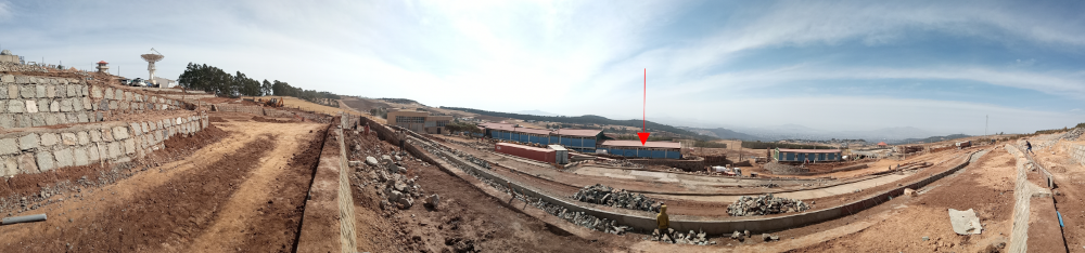
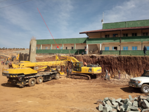
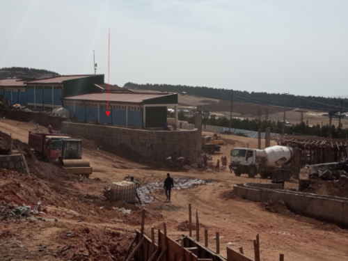
Fig. 1: Rear panoramic (top), front (bottom left), and back (bottom right) views of the ENTOTO Observatory Research Center currently undergoing major construction. The red arrows indicate the room where the MNM is currently installed.

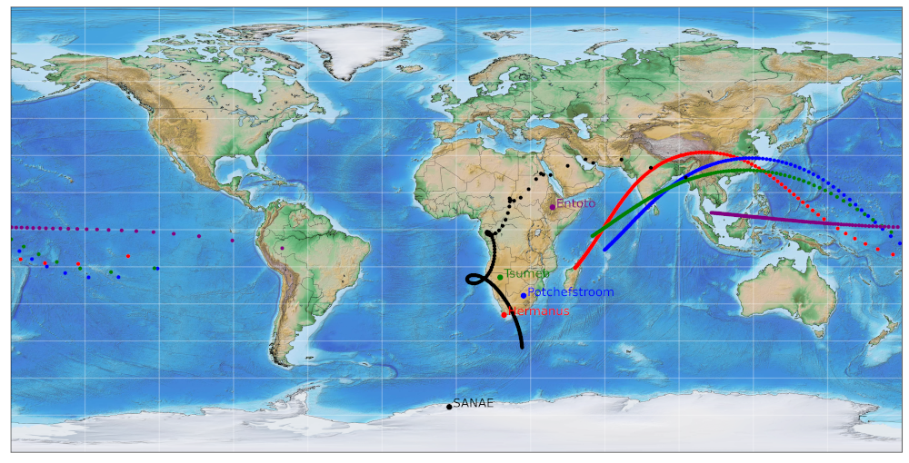
Fig. 2: The asymptotic cones of vertically incident primary particles reaching each monitor in the African neutron monitor network.

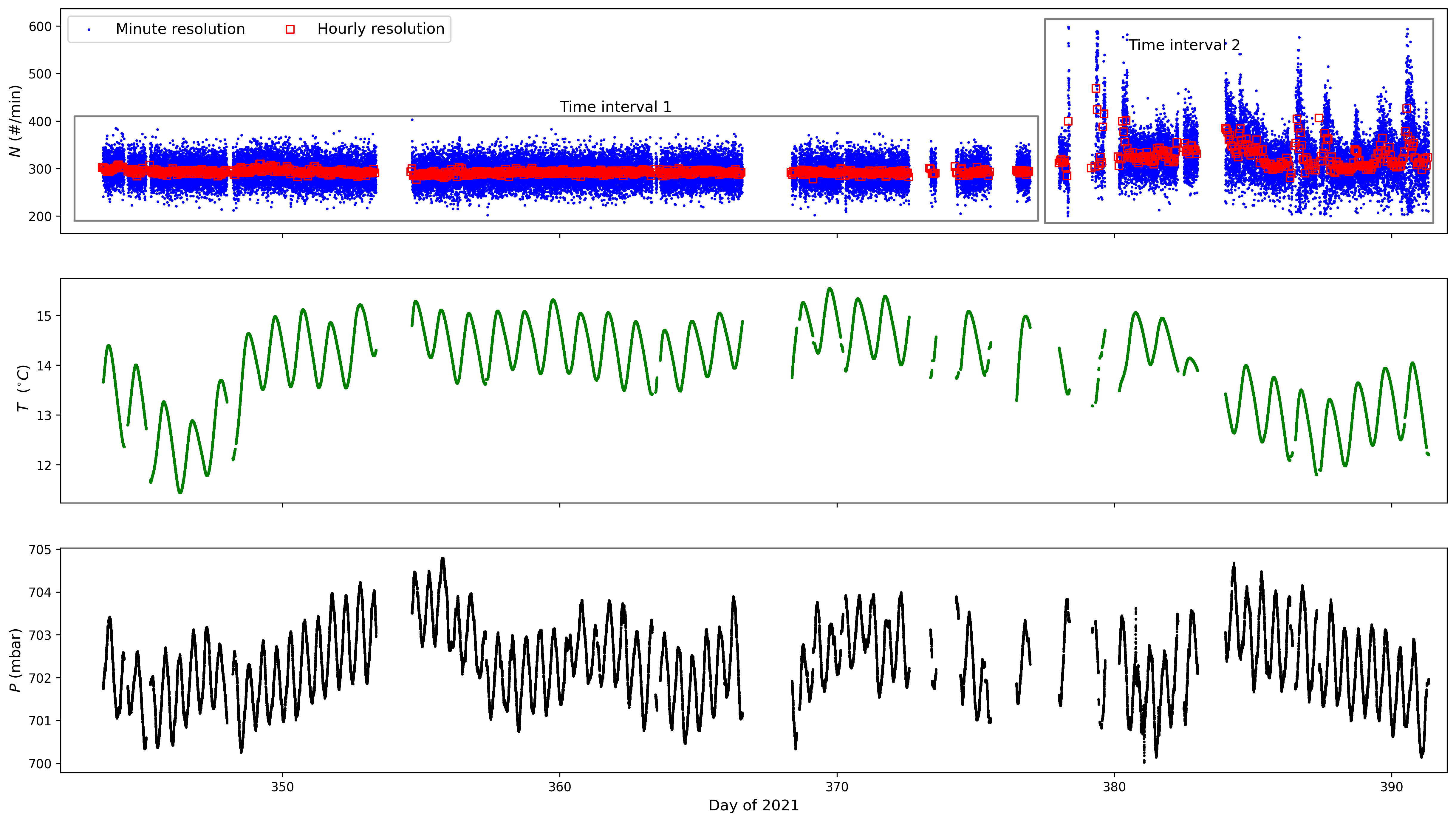
Fig. 3: The top panel shows the minute-averaged (blue) and hourly-averaged (red) count rate as a function of time. The middle and bottom panels show the measured temperature and pressure, respectively.

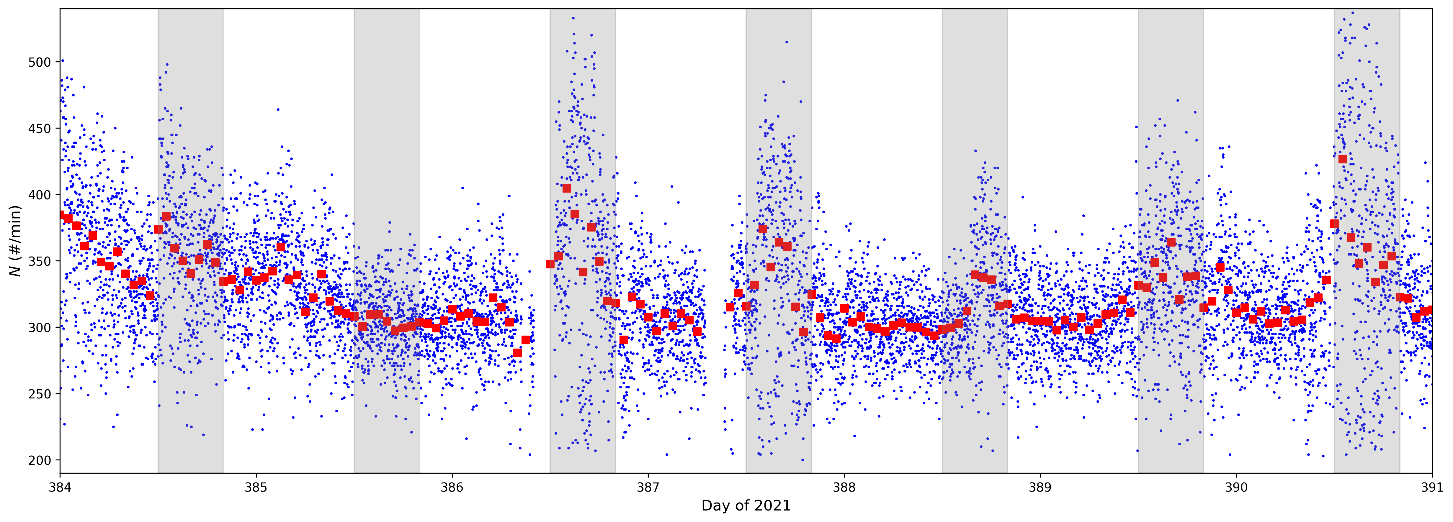
Fig. 4: A zoom in of time interval 2 as identified in Fig. 3.

2 The ENTOTO neutron monitor station

Table 1: Details of the newly established ENTOTO MNM, along with existing NM stations forming the African NM network.

Station	Local time	Latitude	Longitude	Altitude	Cut-off rigidity
ENTOTO, Ethiopia	UTC + 3 hr	9∘ 6’ N	38∘ 48’ E	3175 m.a.s.l.	16 GV
Tsumeb, Namibia	UTC + 2 hr	19∘ 12’ S	17∘ 35’ E	1240 m.a.s.l.	9.2 GV
Potchefstroom, South Africa	UTC + 2 hr	26∘ 41.9’ S	27∘ 5.6’ E	1351 m.a.s.l.	7.2 GV
Hermanus, South Africa	UTC + 2 hr	34∘ 25.5’ S	19∘ 13.5’ E	26 m.a.s.l.	4.9 GV
SANAE, Antarctica	UTC	71∘ 40’ S	2∘ 51’ W	856 m.a.s.l.	0.8 GV

A BF₃ version of the MNM, recently reviewed in detail by Strauss et al. (2020), donated from the North-West University of South Africa to the Space Science and Applications Research and Development department of the Ethiopian Space Science and Technology Institute (ESSTI) of Ethiopia, was recently installed at the premises of the ENTOTO Observatory Research Center (EORC) located in the outskirts of Addis Ababa, the capital city of Ethiopia. Fig. 1 shows recent pictures of this site which is currently undergoing major construction. The red arrows indicate the position where the MNM is currently installed. ENTOTO is in a mountainous landscape that reaches an altitude/elevation of 3200 m.a.s.l. In fact, the peak altitude of 3200 m.a.s.l is reached at the EORC premises. Since the name ENTOTO is associated with the vast and mountainous terrain that surrounds most of the northern and north-western outskirts of Addis Ababa, we have decided to refer to this MNM station as the “ENTOTO Neutron Monitor”, abbreviated as ENTO. Fig. 2 shows the asymptotic cones of acceptance for the African NM network using the model of Smart et al. (2000). The highest rigidity particle considered is 30 GV (the data point closest to the station), decreasing linearly until the cut-off rigidity is reached (data point furthest away from the station). The ENTOTO MNM, being installed very close to the magnetic equator, primarily measures particles incident along the Earth’s equatorial regions. Details of the ENTOTO NM station is summarized in Tab. 1, along with existing NM stations forming the African NM network.

2.1 Unprocessed results

The raw data from the ENTOTO MNM is shown in Fig. 3. The top panel shows the minute-averaged (blue) and hourly-averaged (red) count rate as a function of time with two time intervals identified. These are discussed further in later sections. The average (uncorrected for pressure changes) count rate of the monitor is $\sim 290$/min. The middle and bottom panels show the measured temperature and pressure, respectively. The data gaps is caused by power outages at the installation site.

2.2 Construction noise

During early 2022, major construction unfortunately started at the ENTOTO observatory site. Mechanical vibration and possible electrical interference from these activities are believed to contribute to the higher levels of noise present during time interval 2, identified in Fig. 3. The count rate data from this time interval is shown again in Fig. 4, where the shaded regions indicate times where the majority of the construction occurs: 9:00 - 17:00 local time. Unfortunately this additional noise component cannot be corrected for and the data from time interval 2 is not used for further analysis in the rest of the work.

3 The Neutron monitor waiting time distribution

3.1 Origin of neutron monitor multiplicities

For either of the ³He or BF₃ filling gases, an electrical pulse is produced via a neutron capture process (Knoll, 2010), i.e.

$${}^{10}\mathrm{B}+\mathrm{n} \rightarrow \left\{\begin{array}[]{ccc}^{7}\mathrm{Li}+\alpha+2.78\,\mathrm{MeV}\\ ^{7}\mathrm{Li}^{*}+\alpha+2.30\,\mathrm{MeV}\end{array}\right.$$ (4)

or

$${}^{3}\mathrm{He}+\mathrm{n}\rightarrow\,^{3}\mathrm{H}+\mathrm{p}+0.76\,\mathrm{MeV}$$ (5)

that ionizes a small portion of the filling gas. The pulse-height measured in the NM is therefore independent of energy of the incident atmospheric particles. Low- and high-energy atmospheric hadrons, however, interact with the lead producer in different ways. Low energy protons and neutrons interact with the monitor, and thus the proportional gas, in a random fashion and their detected pulse show a stochastic nature with subsequent pulses unrelated to each other. A high energy neutron or proton, on the other hand, can interact with the lead producer to form a number of low energy evaporation neutrons (e.g. Bieber et al., 2004). These neutrons are observed as a number of pulses over a short period of time, showing a high level of temporal correlation. This is usually expressed in terms of the waiting time distribution (i.e. the time between subsequent pulses observed in the monitor) as the level of multiplicity (i.e. the number of pulses observed in a certain time increment). By thus looking at the waiting time distribution observed by the monitor (examples are shown in the next section) these two components can be distinguished; a low multiplicity component at long waiting times and a high multiplicity, highly correlated, component at short waiting times. By examining the ratio of these components, which we refer to as the correlation ratio, some information of the incident particle spectrum can, in principle, be reconstructed (see e.g. Ruffolo et al., 2016; Mangeard et al., 2016; Banglieng et al., 2020).

3.2 An illustrative example: Lead vs. lead-free neutron monitors

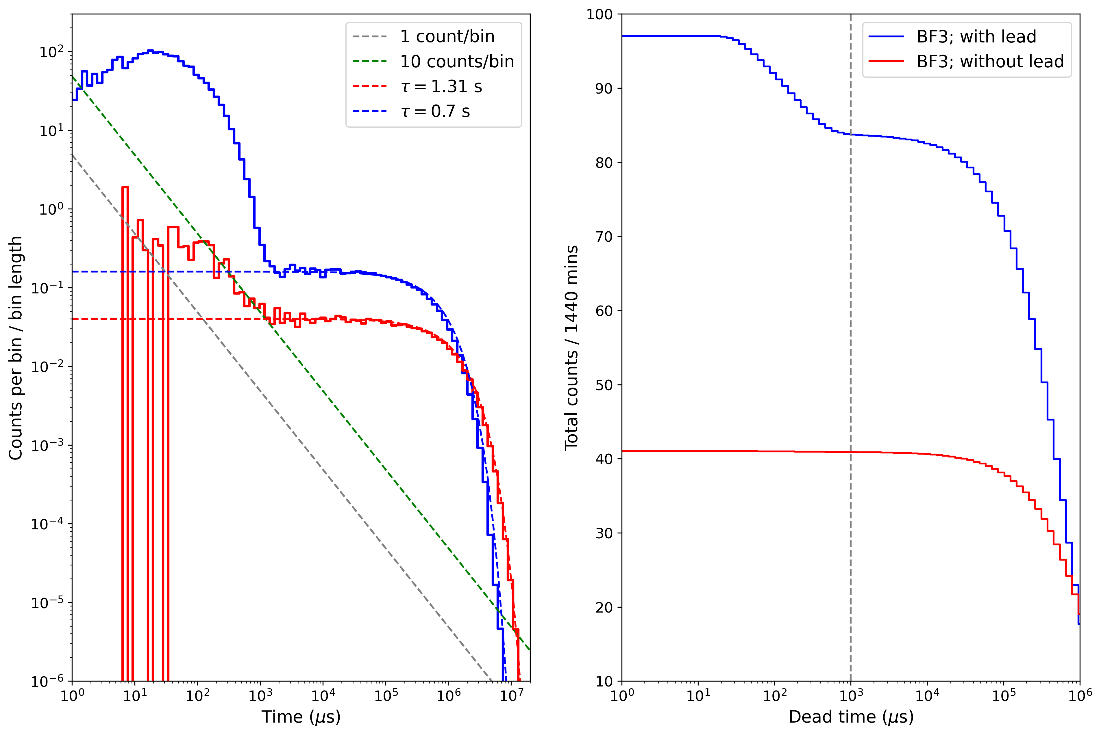
Fig. 5: The waiting time distribution (left panel) and integrated waiting time distribution (right panel) for two identical BF₃-filled mini-NMs; one operated with lead (blue curves) and one without (red curves). In the left panel, the 1 and 10 counts limits are shown (gray and green dashed curves), while the low multiplicity portions of the distributions are fitted with exponential distributions (blue and red dashed curves). The vertical dashed line on the right panel indicates the approximate change from high to low multiplicities observed in the detector with lead at $\sim 1$ms.

To illustrate how the waiting time distribution is formed by different neutron populations, we performed the following test: Two identical BF₃ filled MNMs were placed next to each other in the physics laboratory in Potchefstroom. The MNMs were operated for a number of days to confirm that the electronics were also identical, with identical count rates (within statistical variations) obtained from both monitors. The lead in one monitor was then removed and both MNMs operated for a day. The resulting waiting time distributions (simply calculated as the probability distribution of the time elapsed between successive counts in the detector) are shown in the left panel of Fig. 5, where the low multiplicity (long waiting time) distribution is fitted with the following exponential distribution

$$\mathcal{D}(\Delta t)=\mathcal{D}_{0}\exp\left(\frac{\Delta t-\,^{0}\Delta t}{\tau}\right),$$ (6)

where $\mathcal{D}_{0}$, ${}^{0}\Delta t$, and $\tau$ are fit constants and $\Delta t$ is the waiting time between successive counts (see also the discussion by Ruffolo et al., 2016).

Clearly, the monitor with the lead producer (blue curve in Fig. 5) shows the high multiplicity (high level of temporal correlation) distribution which is absent in the lead-free monitor (red curve in Fig. 5). However, the low multiplicity distributions are also significantly different with a higher count rate observed, even at longer waiting times, for the monitor with lead (roughly a factor of 2). A higher count rate also changes the low multiplicity exponential distribution (see Eq. 6), with the lead monitor well described with a $\tau$ parameter roughly twice that of the lead-free monitor. The low multiplicity part (at longer waiting times) are detected neutrons that are therefore consistent with particles interacting randomly with the detector with the resulting counts unrelated.

In the right panel of Fig. 5, we calculated, using measurements presented in the left panel, the total number of counts measured by these detectors as a function of simulated dead time of the detector, $\Delta T$,

$$\mathcal{C}(\Delta T)=\int_{\Delta T}^{\infty}\mathcal{D}(\Delta t)\Delta t,$$ (7)

which is essentially an integration of the waiting time distribution over all possible waiting times. The vertical dashed line at 1 ms indicates the changeover from the low to the high multiplicity distribution. The leaded monitor has an average count rate of $\sim 95$/min. From the integrated multiplicity distribution we estimate that the low multiplicity (long waiting time) distribution of the monitor with lead has an average count rate of $\sim$80/min while the high multiplicity (short waiting time) distribution contributes at a rate of $\sim$15/min. This suggests that, for the leaded monitor, $\sim$20% of the measured neutrons are high multiplicity neutrons produced in the lead producer by high energy protons and/or neutrons, while the remaining $\sim$80% are low multiplicity neutrons produced either in the lead producer or in the atmosphere. The monitor without lead gives an average count rate of $\sim$40/min which are presumably due to neutrons produced in the atmosphere. This suggests that, for the BF₃ version of the mini-NM located in Potchefstroom, about half of low multiplicity neutrons measured by the leaded monitor are already formed in the atmosphere, contributing with a rate of $\sim$40/min towards the total count rate. It is also instructive to remember that $\sim 90\%$ of the atmospheric particles detected by a typical NM are atmospheric neutrons (Mangeard et al., 2016). Also note that these estimates will be different for different NM designs and will depend on the local environment and incident particle spectrum.

4 Measuring and quantifying the waiting time distribution

4.1 Correlated and uncorrelated count rates

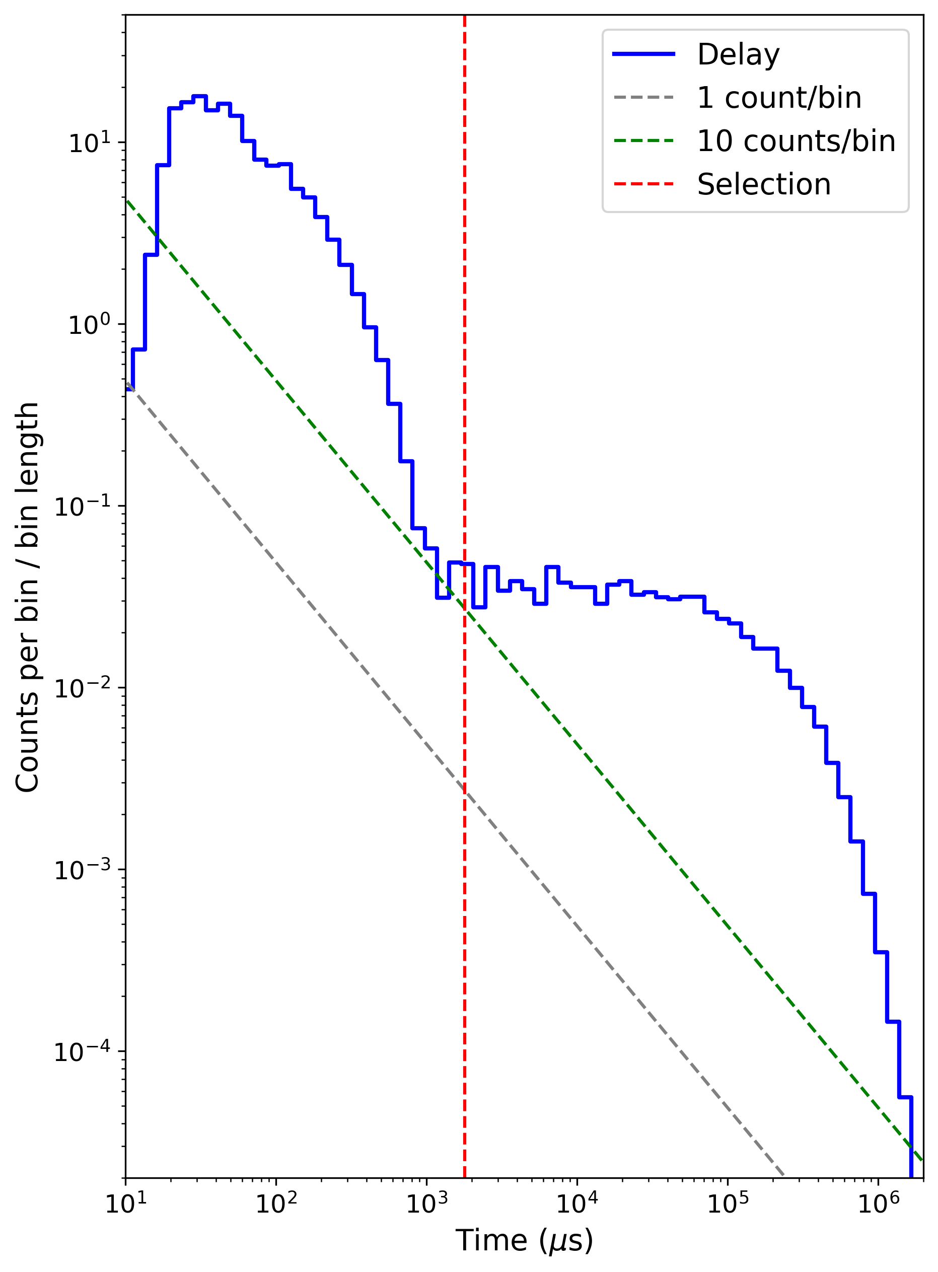
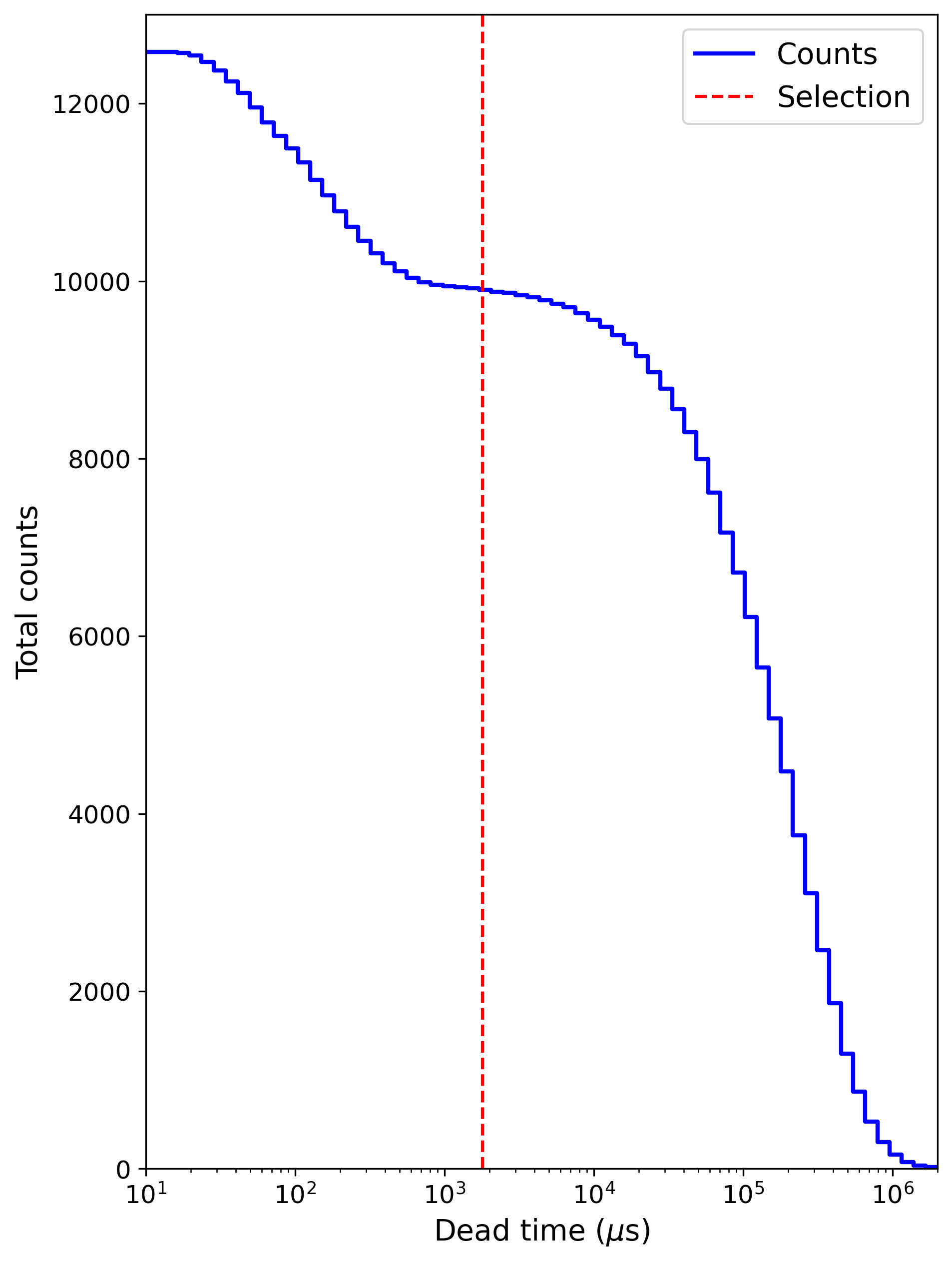
Fig. 6: Similar to Fig. 5, but now calculate using a hour’s measurements of the ENTOTO MNM.

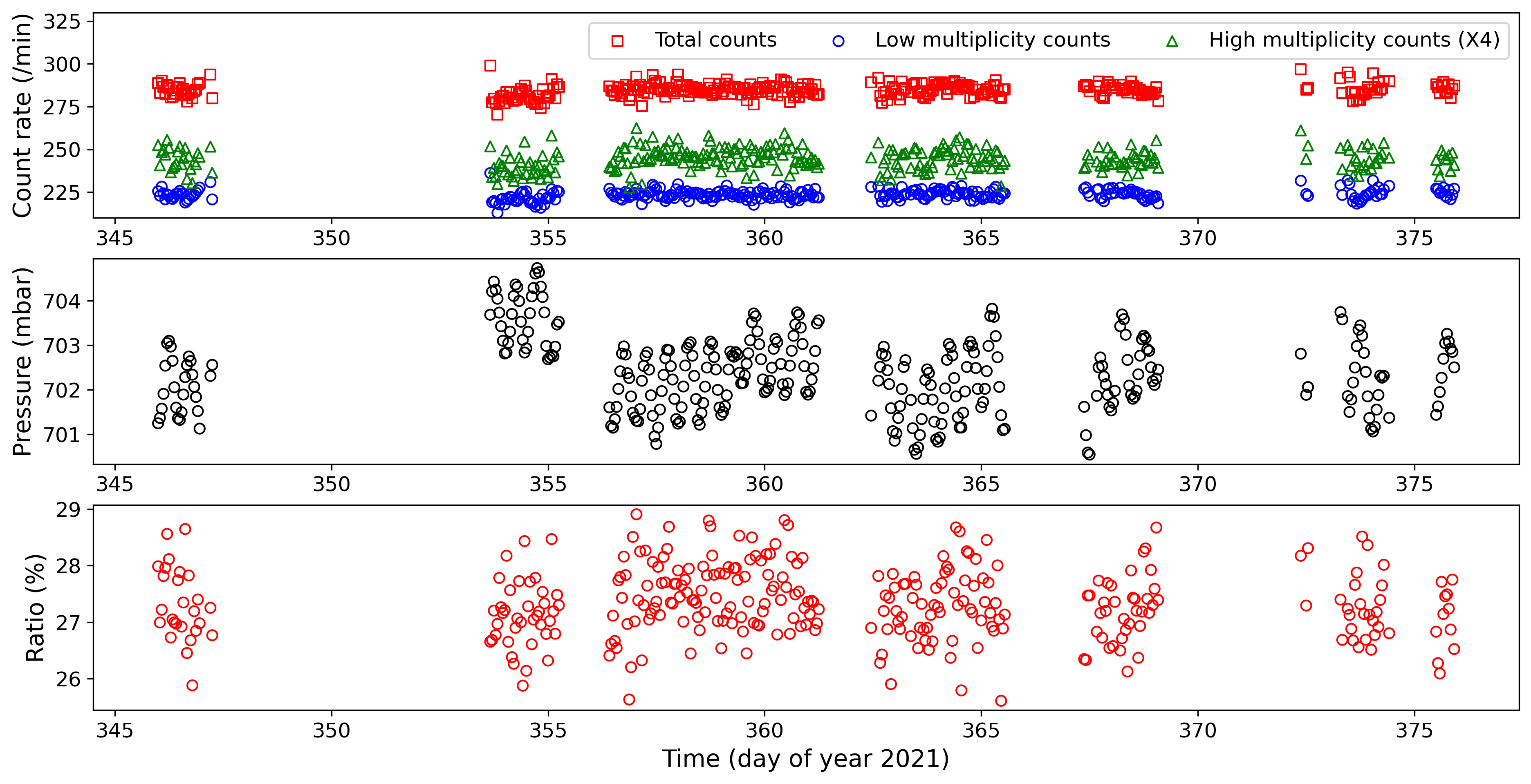
Fig. 7: The top panel shows hourly averaged count rates for the low multiplicity (blue), high multiplicity (green, multiplied by a factor of 4), and the total distributions. The middle panel shows the hourly averaged pressure and the bottom panel the ratio of the high multiplicity to low multiplicity count rates, the so-called correlation ratio.

The waiting time distribution as measured by the ENTOTO MNM is shown in Fig. 6, with a similar format as Fig. 5. As expected, the uncorrelated low multiplicity (long waiting times, $>2$ ms) and correlated high multiplicity (short waiting times, $<2$ ms) distributions can be identified. The vertical red dashed line in Fig. 6, at $\Delta T^{\prime}=2$ ms, indicates the assumed change in distribution and used for the rest of the work to separate the two distributions.

We now calculate the hourly waiting time distribution, similar to Fig. 6, for each hour in time interval 1 (as defined in Fig. 3). From these distributions, we calculate the hourly count rate of the high multiplicity component as

$$\mathcal{C}_{\mathrm{high}}(t,\Delta T^{\prime})=\int_{0}^{\Delta T^{\prime}}\mathcal{D}(t,\Delta t)\Delta t,$$ (8)

the count rate of the low multiplicity component as

$$\mathcal{C}_{\mathrm{low}}(t,\Delta T^{\prime})=\int_{\Delta T^{\prime}}^{\infty}\mathcal{D}(t,\Delta t)\Delta t,$$ (9)

and the total count rate as

$$\mathcal{C}_{\mathrm{total}}(t)=\mathcal{C}_{\mathrm{low}}(t,\Delta T^{\prime})+\mathcal{C}_{\mathrm{high}}(t,\Delta T^{\prime})=\int_{0}^{\infty}\mathcal{D}(t,\Delta t)\Delta t.$$ (10)

These different count rates are shown as a function of time in the top panel of Fig. 7 with the hourly averaged pressure in the middle panel. Note that for these calculations we only use complete hourly intervals with a full 60 minutes of measurements. The data is therefore much more sparse than the minute-averaged measurements shown in Fig. 3 which contains a large number of data gaps. In the bottom panel we calculate the so-called correlation ratio, as

$$\mathcal{R}(t,\Delta T^{\prime})=\frac{\mathcal{C}_{\mathrm{high}}(t,\Delta T^{\prime})}{\mathcal{C}_{\mathrm{low}}(t,\Delta T^{\prime})}\times 100\%,$$ (11)

which we expect to be a proxy for the spectral index of the incident atmospheric particles. The data presented here gives a ratio of $\sim 27\%$ when using a value of $\Delta T^{\prime}=$ 2ms. As this is essentially the ratio of correlated to uncorrelated counts in the monitor, we expect the ratio to increase (more correlated, high multiplicity counts) as the spectrum of incident particles become harder (more high energy particles). We test for any pressure dependence of the different count rates, and the ratio thereof, in the next section.

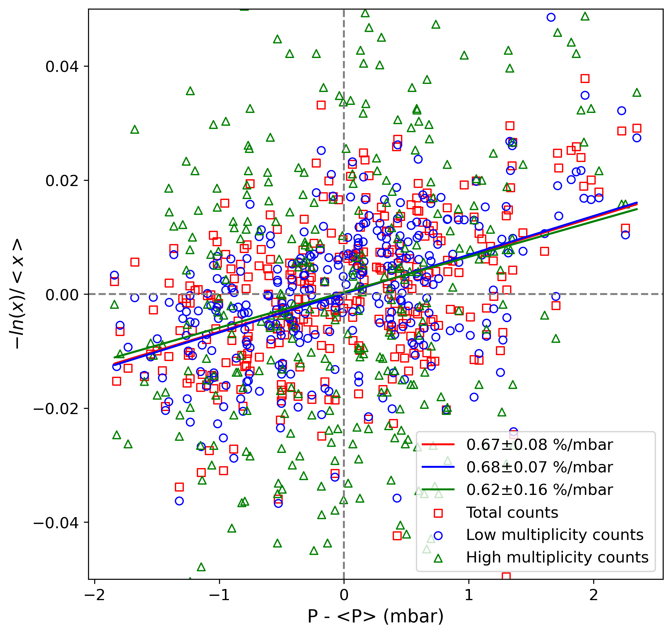
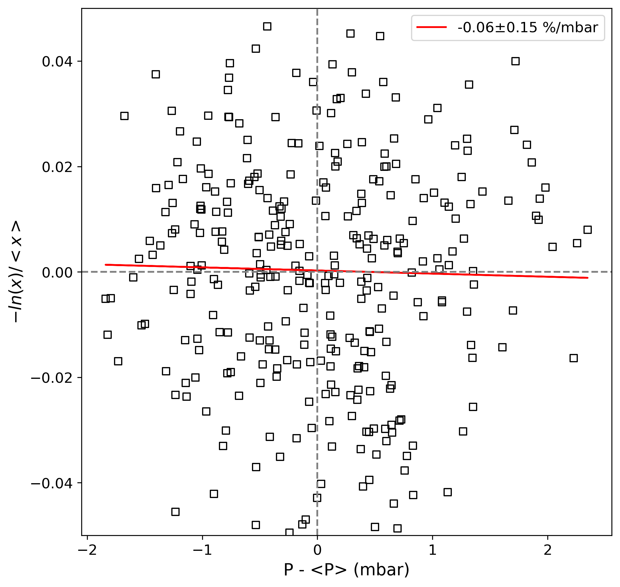
Fig. 8: The left panel shows the barometric correction applied separately for the 3 different count rates identified in Sec. 4.1, while the right panel shows the same calculation for the correlation ratio.

4.2 Pressure corrections

Assuming the standard exponential correlation between the count rate and atmospheric pressure, the hourly count rate is expected to vary with varying atmospheric pressure, $P$, as

$$\mathcal{C}_{\mathrm{x}}=\langle\mathcal{C}_{\mathrm{x}}\rangle\exp\left(-\beta_{\mathrm{x}}\Delta P\right),$$ (12)

where $x$ refers to either the low, high, or total count rate, $\Delta P=P-\langle P\rangle$, and $\langle\cdot\rangle$ indicates long-term averaging. The barometric coefficients, $\beta_{\mathrm{x}}$, for the different count rates are calculated in the left panel of Fig. 8 as the gradient of a linear regression, with resulting values included in the legend where the colour of the regresion line corresponds to that of the data points. As the high multiplicity counts are produced by higher energy atmospheric particles, we expect the corresponding barometric coefficient to be smaller than of the low multiplicity component, based on the work of Tirado-Bueno et al. (2021). While there might be an indication of this, the different coefficients are the same within the (relatively large) fit errors.

The correlation ratio is expected to have a pressure dependence of the form,

$$\mathcal{R}=\frac{\mathcal{C}_{\mathrm{high}}}{\mathcal{C}_{\mathrm{low}}}=\frac{\langle\mathcal{C}_{\mathrm{high}}\rangle}{\langle\mathcal{C}_{\mathrm{low}}\rangle}\exp\left[-\left(\beta_{\mathrm{high}}-\beta_{\mathrm{low}}\right)\Delta P\right],$$ (13)

with an effective pressure coefficient of $\beta=\beta_{\mathrm{high}}-\beta_{\mathrm{low}}$. The pressure dependence of $\mathcal{R}$ is therefore expected to be weaker than that of the individual count rates. This is confirmed in the right panel of Fig. 8 where we apply a similar pressure correction to the correlation ratio. Within the fit errors we find the correlation ratio to be independent of pressure changes.

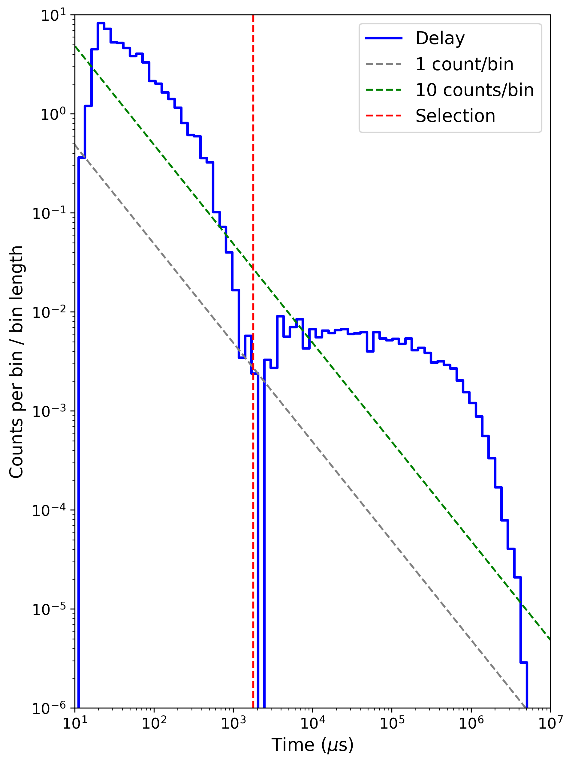
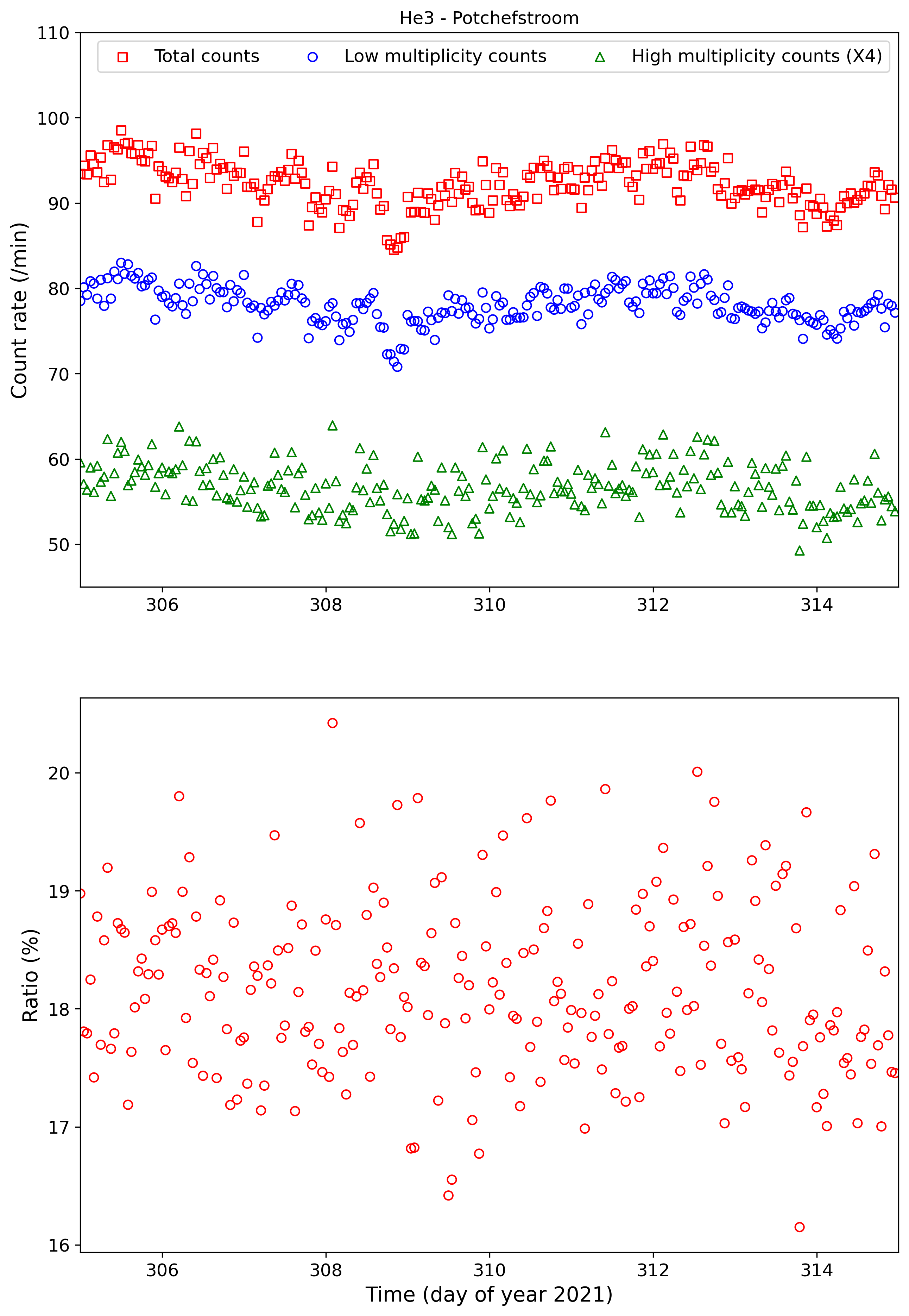
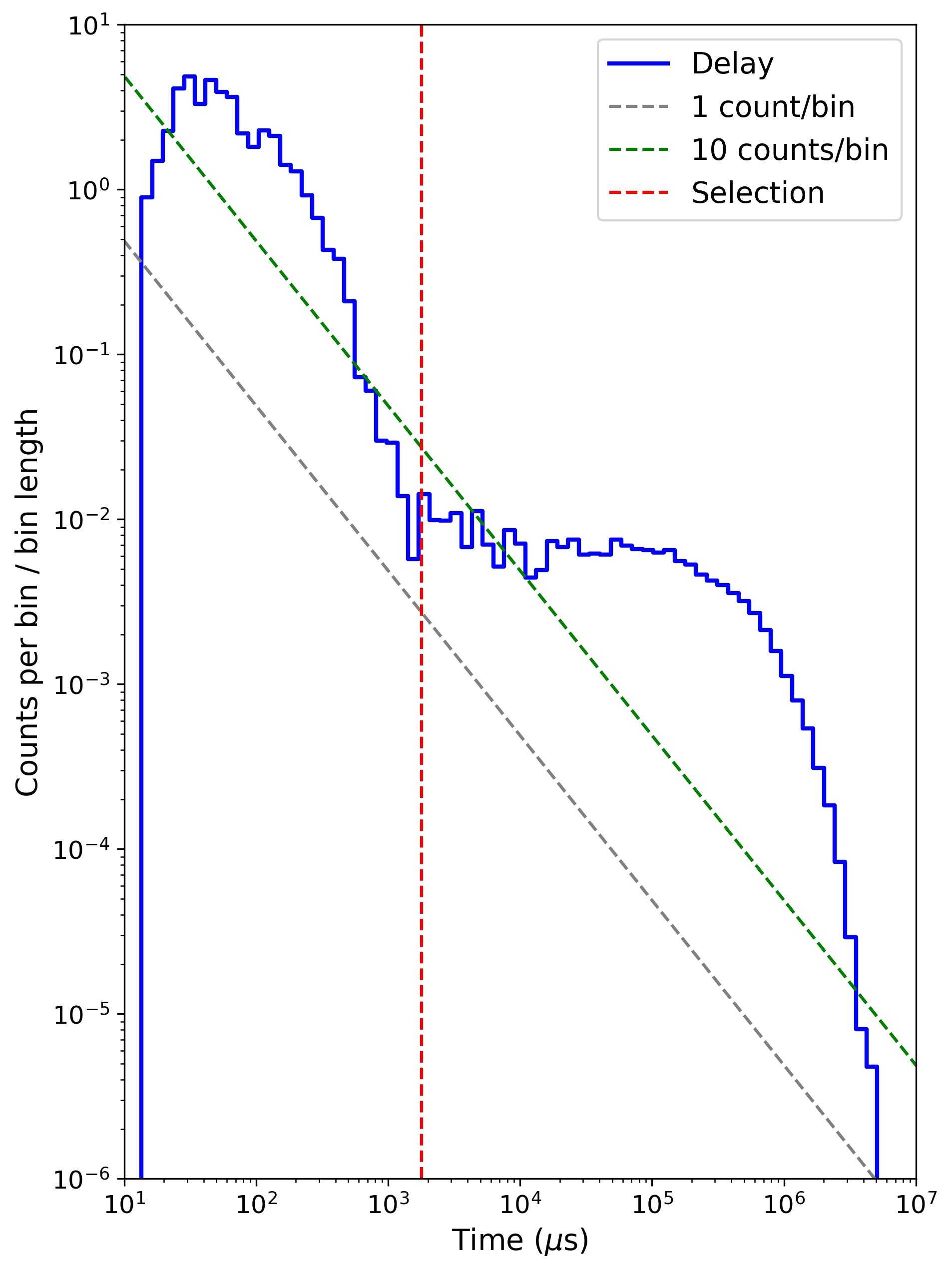
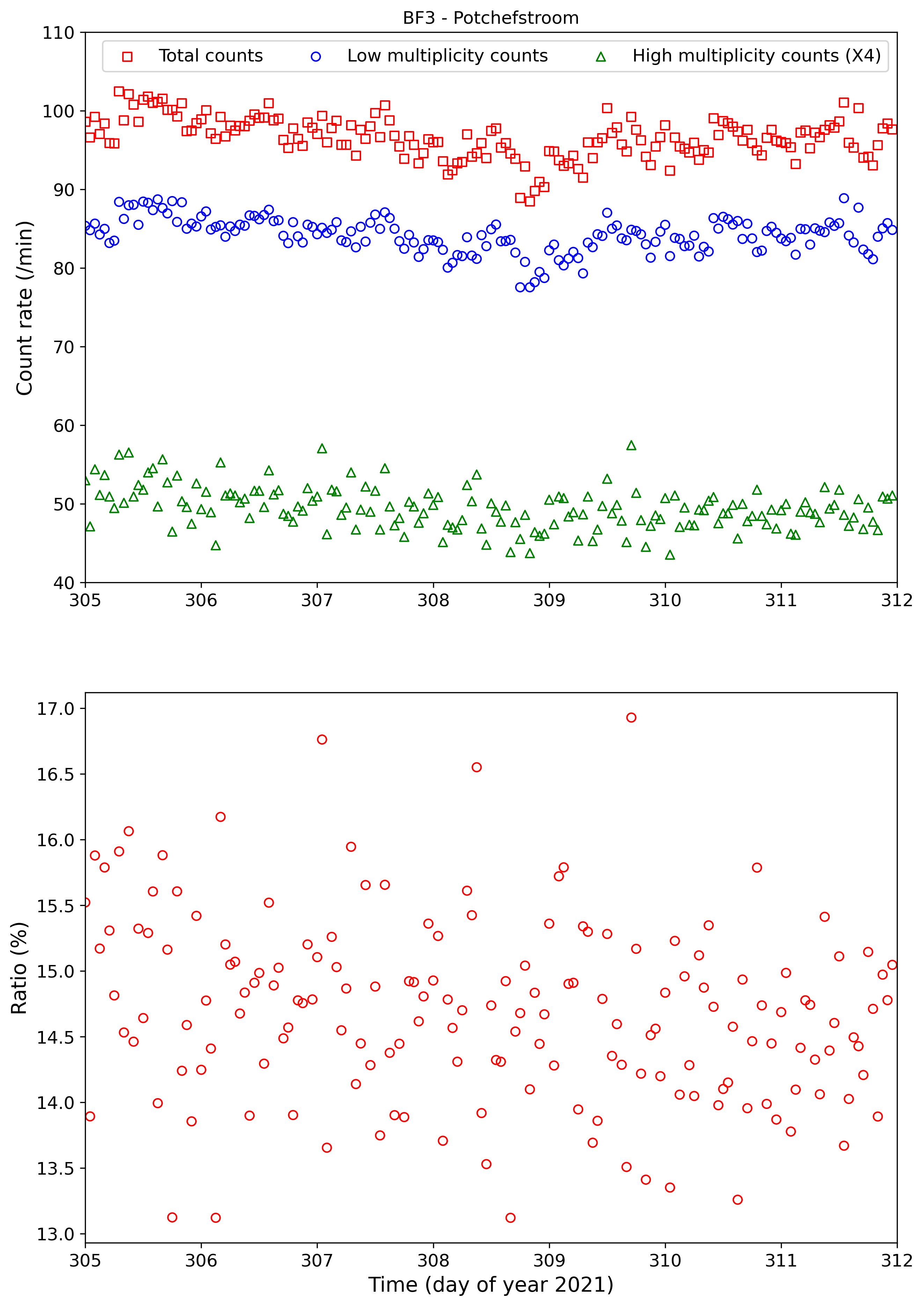
Fig. 9: Similar to Figs. 6 and 7, but now for a ³He (top panels) and a BF₃ (bottom panels) MNM housed in the laboratory in Potchefstroom.

4.3 Comparison with other monitors

We end the analysis presented here with a comparison between the ENTOTO waiting time distribution and the time distributions measured by a ³He and BF₃ leaded MNM housed in the laboratory in Potchefstroom. The results for these MNMs are shown in Fig. 9. Of course, the waiting time distributions show similarities with that of ENTOTO, with the change between high and low multiplicity distributions again occurring close to $\sim 2$ ms. The right panels of the figure show the behaviour of the different count rates, and the correlation ratio, as a function of time. For the ³He tube, the ratio is $\sim 18\%$, and for the BF₃ tube it is $\sim 14\%$. It should be kept in mind that the ³He version of the MNM has a thicker lead producer (due to a thinner tube) than the BF₃ version which might explain the additional $\sim 3\%$ of high-multiplicity neutrons detected.

5 Summary, conclusions, and outlook

We have discussed a newly established MNM station installed at the ENTOTO Observatory Research Center outside of Addis Ababa, Ethiopia. Preliminary data from the ENTOTO MNM is shown and discussed, with a special focus on characterising the waiting time distribution.

Using the waiting time distribution, as observed by this new station, we calculated the ratio of correlated to uncorrelated counts as a proxy for the spectral index of the incident atmospheric particles. While similar proxies were used in the past, e.g. the leader fraction of Ruffolo et al. (2016), our correlation ratio, as defined here, is a natural characterization of the waiting time distribution as measured by our MNMs. We hope to also calculate the correlation ratio for other NMs in future, as well track how this ratio changes during temporal events such as ground level enhancement and Forbush decreases.

We calculated the pressure dependence of different count rates of the ENTOTO MNM, and found very similar values for both the correlated and uncorrelated count rates. This suggests that the pressure dependence of correlation ratio will be rather weak and, for typical MNM count rates, probably negligible as the uncertainty in the measurements is dominated by the statistical errors associated with low count rates.

The ENTOTO MNM, at a cut-off rigidity of $\sim 16$ GV, has a current correlation ratio of $\sim 27\%$. We also calculated this quantity for two MNMs (with a BF₃ and ³He tube) currently undergoing testing at the laboratory in Potchefstroom. These MNMs recorded ratios of $\sim 14\%$ and $\sim 18\%$, respectively. Given the fact that Potchefstroom has an approximate cut-off rigidity of only $\sim 7$ GV, the higher ENTOTO correlation ratio can be explained by the fact that the ENTOTO MNM measures higher rigidity particles, resulting in a higher ratio of correlated neutrons being detected inside the monitor, partially validating our proposal that this ratio will serve as a proxy for the spectral shape of the incident atmospheric particles. We will continue to investigate the use of the correlation ratio for this purpose, especially during transient phenomena such as Forbush decreases, and report such results in due course.

References

- Banglieng et al. (2020) Banglieng, C., Janthaloet, H., Ruffolo, D., Sáiz, A., Mitthumsiri, W., Muangha, P., Evenson, P., Nutaro, T., Pyle, R., Seunarine, S., Madsen, J., Mangeard, P. S., & Macatangay, R. (2020). Tracking Cosmic-Ray Spectral Variation during 2007-2018 Using Neutron Monitor Time-delay Measurements. The Astrophysical Journal, 890(1), 21. doi:10.3847/1538-4357/ab6661.
- Bieber et al. (2004) Bieber, J. W., Clem, J. M., Duldig, M. L., Evenson, P. A., Humble, J. E., & Pyle, R. (2004). Latitude survey observations of neutron monitor multiplicity. Journal of Geophysical Research (Space Physics), 109(A12), A12106. doi:10.1029/2004JA010493.
- Clem & Dorman (2000) Clem, J. M., & Dorman, L. I. (2000). Neutron Monitor Response Functions. Space Science Reviews, 93, 335–359. doi:10.1023/A:1026508915269.
- Harris et al. (2020) Harris, C. R., Millman, K. J., van der Walt, S. J., Gommers, R., Virtanen, P., Cournapeau, D., Wieser, E., Taylor, J., Berg, S., Smith, N. J., Kern, R., Picus, M., Hoyer, S., van Kerkwijk, M. H., Brett, M., Haldane, A., del Río, J. F., Wiebe, M., Peterson, P., Gérard-Marchant, P., Sheppard, K., Reddy, T., Weckesser, W., Abbasi, H., Gohlke, C., & Oliphant, T. E. (2020). Array programming with NumPy. Nature, 585, 357–362. doi:10.1038/s41586-020-2649-2.
- Heber et al. (2015) Heber, B., Galsdorf, D., Gieseler, J., Herbst, K., Walter, M., Stoessl, A., Moraal, H., Krüger, H., & Benade, G. (2015). Mini neutron monitor measurements at the Neumayer III station and on the German research vessel Polarstern. In 34th International Cosmic Ray Conference (ICRC2015) (p. 122). volume 34 of International Cosmic Ray Conference.
- Hunter (2007) Hunter, J. D. (2007). Matplotlib: A 2d graphics environment. Computing in Science & Engineering, 9(3), 90–95. doi:10.1109/MCSE.2007.55.
- Knoll (2010) Knoll, G. F. (2010). Radiation Detection and Measurement, 4th ed.. New York, NY: Wiley.
- Krüger et al. (2008) Krüger, H., Moraal, H., Bieber, J. W., Clem, J. M., Evenson, P. A., Pyle, K. R., Duldig, M. L., & Humble, J. E. (2008). A calibration neutron monitor: Energy response and instrumental temperature sensitivity. Journal of Geophysical Research (Space Physics), 113(A8), A08101. doi:10.1029/2008JA013229.
- Mangeard et al. (2016) Mangeard, P. S., Ruffolo, D., Sáiz, A., Nuntiyakul, W., Bieber, J. W., Clem, J., Evenson, P., Pyle, R., Duldig, M. L., & Humble, J. E. (2016). Dependence of the neutron monitor count rate and time delay distribution on the rigidity spectrum of primary cosmic rays. Journal of Geophysical Research (Space Physics), 121(12), 11,620–11,636. doi:10.1002/2016JA023515.
- Mishev & Usoskin (2020) Mishev, A., & Usoskin, I. (2020). Current status and possible extension of the global neutron monitor network. Journal of Space Weather and Space Climate, 10, 17. doi:10.1051/swsc/2020020. arXiv:2005.12621.
- Mishev et al. (2020) Mishev, A. L., Koldobskiy, S. A., Kovaltsov, G. A., Gil, A., & Usoskin, I. G. (2020). Updated Neutron-Monitor Yield Function: Bridging Between In Situ and Ground-Based Cosmic Ray Measurements. Journal of Geophysical Research (Space Physics), 125(2), e27433. doi:10.1029/2019JA027433.
- Poluianov et al. (2015) Poluianov, S., Usoskin, I., Mishev, A., Moraal, H., Kruger, H., Casasanta, G., Traversi, R., & Udisti, R. (2015). Mini Neutron Monitors at Concordia Research Station, Central Antarctica. Journal of Astronomy and Space Sciences, 32(4), 281--287. doi:10.5140/JASS.2015.32.4.281.
- Ruffolo et al. (2016) Ruffolo, D., Sáiz, A., Mangeard, P. S., Kamyan, N., Muangha, P., Nutaro, T., Sumran, S., Chaiwattana, C., Gasiprong, N., Channok, C., Wuttiya, C., Rujiwarodom, M., Tooprakai, P., Asavapibhop, B., Bieber, J. W., Clem, J., Evenson, P., & Munakata, K. (2016). Monitoring Short-term Cosmic-ray Spectral Variations Using Neutron Monitor Time-delay Measurements. Astrophysical Journal, 817(1), 38. doi:10.3847/0004-637X/817/1/38.
- Simpson (2000) Simpson, J. A. (2000). The Cosmic Ray Nucleonic Component: The Invention and Scientific Uses of the Neutron Monitor - (Keynote Lecture). Space Science Reviews, 93, 11--32. doi:10.1023/A:1026567706183.
- Smart et al. (2000) Smart, D. F., Shea, M. A., & Flückiger, E. O. (2000). Magnetospheric Models and Trajectory Computations. Space Science Reviews, 93, 305--333. doi:10.1023/A:1026556831199.
- Stoker (1985) Stoker, P. H. (1985). Spectra of Solar Proton Ground Level Events Using Neutron Monitor and Neutron Moderated Detector Recordings. In 19th International Cosmic Ray Conference (ICRC19), Volume 4 (p. 114). volume 4 of International Cosmic Ray Conference.
- Strauss et al. (2020) Strauss, R. D., Poluianov, S., van der Merwe, C., Krüger, H., Diedericks, C., Krüger, H., Usoskin, I., Heber, B., Nndanganeni, R., Blanco-Ávalos, J., García-Tejedor, I., Herbst, K., Caballero-Lopez, R., Moloto, K., Lara, A., Walter, M., Giday, N. M., & Traversi, R. (2020). The mini-neutron monitor: a new approach in neutron monitor design. Journal of Space Weather and Space Climate, 10, 39. doi:10.1051/swsc/2020038.
- Strauss et al. (2021) Strauss, R. D., van der Merwe, C., Diedericks, C., Krüger, H., Krüger, H. G., Moloto, K. D., Lotz, S., & Mosotho, G. M. (2021). The updated SANAE neutron monitor. Advances in Space Research, 68(6), 2661--2675. doi:10.1016/j.asr.2021.05.032. arXiv:2107.14289.
- Tirado-Bueno et al. (2021) Tirado-Bueno, E., Mendoza-Torres, J. E., & de Mendonça, R. R. S. (2021). Barometric coefficient dependence on the geomagnetic cutoff rigidity of neutron monitors. Advances in Space Research, 68(6), 2631--2642. doi:10.1016/j.asr.2021.04.034.
- Usoskin et al. (2015) Usoskin, I., Poluianov, S., Moraal, H., Krüger, H., Casasanta, G., Traversi, R., & Udisty, R. (2015). A mini neutron monitor in Central Antarctica (Dome Concordia). In 34th International Cosmic Ray Conference (ICRC2015) (p. 217). volume 34 of International Cosmic Ray Conference.
- Zreda et al. (2012) Zreda, M., Shuttleworth, W. J., Zeng, X., Zweck, C., Desilets, D., Franz, T., & Rosolem, R. (2012). Cosmos: the cosmic-ray soil moisture observing system. Hydrology and Earth System Sciences, 16(11), 4079--4099. URL: https://hess.copernicus.org/articles/16/4079/2012/. doi:10.5194/hess-16-4079-2012.