A Global Asymptotic Convergent Observer for SLAM

Abstract

This paper examines the global convergence problem of SLAM algorithms, an issue that faces topological obstructions. This is because the state-space of attitude dynamics is defined on a non-contractible manifold: the special orthogonal group of order three $SO(3)$. Therefore, this paper presents a novel, gradient-based hybrid observer to overcome these topological obstacles. The Lyapunov stability theorem is used to prove the globally asymptotic convergence of the proposed algorithm. Finally, comparative analyses of two simulations were conducted to evaluate the performance of the proposed scheme and to demonstrate the superiority of the proposed hybrid observer to a smooth observer.

I Introduction

Simultaneous Localization and Mapping (SLAM) is a well-known highly nonlinear problem which many previous studies have examined [1]. This estimation problem has an extensive variety of applications, ranging from unmanned aerial vehicles (UAV) to underwater robotics. Likewise, the co-dependence of environmental mapping and pose estimation makes the problem of significant theoretical interest. In the SLAM problem, a mobile robot tries to construct a map of an environment while simultaneously estimating its pose (i.e., attitude and position) [2]. Different types of estimation techniques have been applied to the SLAM problem, including Kalman-type filters [3] and geometric nonlinear observers [4].

As mentioned above, the Kalman filter and its variants are the estimation algorithms that have most frequently been employed to solve SLAM [5]. Nevertheless, Kalman-type filters suffer from some serious shortcomings; for example, their performance depends on the prior information regarding noise statistics and initial values; consistency is also an issue [6]. Several previous studies have addressed these limitations [7]. For example, [8] introduced a new unscented Kalman-type filter (UKF), called observability-constrained (OC)-UKF, to address two key restrictions of UKF: the computational cost in high-dimension systems and the inconsistency problem. A right invariant extended Kalman filter (RI-EKF) based on a new Lie group structure has also been presented by [9] to solve the inconsistency issue. Masreliez-Martin UKF (MMUKF) has been presented in [10] to resolve the problems related to stability and tracking accuracy. In this strategy, an adaptive factor was included to calculate the process noise covariance matrix, and a dynamic model of the robot was utilized to predict the locations of the robot and of landmarks. The inconsistency of EKF-SLAM has also been investigated by [11]; here, the filter Jacobians are determined utilizing the first-ever accessible estimates for each state to preserve the dimensions of the observable subspace. [12] used a combination of EKF and a particle filter to address the SLAM problem. In this method, the particle filter determines the position of the mobile robot, and the EKF estimates the position of the environment. The performance of the UKF-SLAM was further developed by [13], who rendered an adaptive random search maximization scheme to adapt the scaling parameter. To further improve the performance of the standard UKF-SLAM and reduce its dependency on prior knowledge, a robust SLAM has also been developed based on $H_{\infty}$ square root UKF [14].

One recently adopted technique for solving the SLAM problem is the use of geometric nonlinear observers. In these strategies, observers are directly designed in matrix Lie groups, including $SE_{1+n}(3)$ and $SLAM_{n}(3)$. For instance, [15] used a gradient-based observer in the underlying Lie group; the innovation term was derived from the descent direction of an error function. Utilizing group speed and landmark measurements, a geometric nonlinear observer has been introduced that evolves directly on the matrix Lie group $SE_{1+n}(3)$ [16]. Furthermore, [17] developed a geometric nonlinear observer directly on the manifold of the Lie group $SLAM_{n}(3)$. This proposed observer could guarantee predefined performance parameters and remove the unspecified bias in velocity measurements by using measurements of inertial measurement unit (IMU), group velocity, and landmarks. In a continuation of previous work, the authors have developed the observer by diminishing the boundaries of the error function to ensure faster convergence on the origin [18]. The SLAM manifold has been introduced to develop the matrix Lie group $SLAM_{n}(3)$ for the SLAM problem in [19]. Consequently, a global asymptotic stable observer has also been derived on the suggested manifold to solve SLAM in dynamic environments.

Alongside the SLAM problem, Visual SLAM (VSLAM) has also received significant attention. VSLAM is a specific case of SLAM in which a monocular camera provides the measurements. Van Goor et al. proposed a new Lie group called $VSLAM_{n}(3)$ and derived an almost globally asymptotically stable observer on $VSLAM_{n}(3)$ [20]. The introduced observer utilized decoupled gain matrices for each landmark and employed a new cost function to calculate innovations in the robot’s pose. In addition, [21] continues the authors’ prior work; here, a gradient-based observer with almost global stability has been designed in the $VSLAM_{n}(3)$ Lie group. Van Goor’s et al. [20] work has been further developed in [22] with the introduction of equivariant group actions. The suggested nonlinear equivariant observer’s almost semi-global convergence is its most important feature.

Although the observers described above have a number of advantages, they also share a significant shortcoming. To the best of the authors’ knowledge, most state-of-the-art observers ensure almost global stability [23]. This is because the special orthogonal group of order three $SO(3)$ is a non-contractible manifold [24]. Hence, there exists a set with Lebesgue measure zero from which the estimation error cannot converge to zero. Hybrid systems have therefore been used to overcome this topological obstruction and to derive observers with global stability on $SO(3)$ [25], $SE(3)$ [26], and $SE_{2}(3)$ [27]. For example, two hybrid observers were introduced in [28]; the first observer uses fixed gains, while the second uses variable gains by solving a continuous Riccati equation. Wang et al. [29] expands on the authors’ previous work; here, the same strategy has been used to develop two hybrid observers. In contrast to previous observers, these observers do not need information about the gravity vector and can overcome the difficulty in estimation under intermittent landmark measurements.

In light of the shortcomings of previous solutions, the present paper addresses the problem of designing an observer with global stability for SLAM. Here, a new, gradient-based hybrid observer is introduced on the $SE_{1+n}(3)$ manifold to solve the SLAM problem. The present article is divided into five sections, including the introduction. Section 2 provides the preliminary mathematical notation, SLAM kinematics and measurements equations, and the basic background on hybrid systems. The proposed hybrid observer is described in section 3. Section 4 illustrates the results of simulations in which the proposed observer is compared to a smooth observer. Finally, section 6 summarizes the paper and provides some concluding remarks.

II Preliminaries

II-A Notation

This paper denotes the sets of real, nonnegative real, and natural numbers by $\mathbb{R}$, $\mathbb{R}_{\geq 0}$, and $\mathbb{N}$, respectively. ${{\mathbb{R}}^{n}}$ represents $n$-dimensional Euclidean space, where $\{e_{i}\}_{1\leq i\leq n}\subset{{\mathbb{R}}^{n}}$ is the canonical basis of ${{\mathbb{R}}^{n}}$. $\left\|x\right\|=\sqrt{\left\langle x,x\right\rangle}$ denotes the two-norm of a vector where $\left\langle x,y\right\rangle:={{x}^{T}}y$ is the inner products of vectors $x,y\in{{\mathbb{R}}^{n}}$ and ${{\left\|x\right\|}_{\mathcal{A}}}:={{\min}_{y\in\mathcal{A}}}\left\|x-y\right\|$. The trace, determinant, and transpose of a matrix $A\in\mathbb{R}^{n\times n}$ are denoted by $\text{tr}(A)$, $\text{det}(A)$, and $A^{T}$, respectively. Moreover, $\left\|A\right\|_{F}=\sqrt{\left\langle A,A\right\rangle}$ is the Frobenius norm of $A$, where $\left\langle A,B\right\rangle:=\text{tr}(A^{T}B)=(\text{vec}A)^{T}(\text{vec}B)$, and $\text{vec}A=[Ae_{1}\ldots Ae_{n}]^{T}$ is the vectorization of $A$. The attitude of a rigid body is denoted by $R\in SO(3)$, where $SO(3):=\{R\in\mathbb{R}^{3\times 3}:R^{T}R=RR^{T}=I,\text{det}(R)=1\}$ is the special orthogonal group of order three, and $\mathfrak{so}(3)=\{A\in\mathbb{R}^{3\times 3}:A^{T}=-A\}$ is the Lie algebra of $SO(3)$. In this paper, $SE_{1+n}(3):=\{\mathcal{X}=\Psi(R,p,\eta):R\in SO(3),p\in\mathbb{R}^{3},\eta\in\mathbb{R}^{3\times n}\}$ represents the matrix Lie group. Throughout this paper, the following identities are used frequently.

$$\begin{split}&\Gamma(y)=\left[\begin{matrix}0&-{{y}_{3}}&{{y}_{2}}\\ {{y}_{3}}&0&-{{y}_{1}}\\ -{{y}_{2}}&{{y}_{1}}&0\\ \end{matrix}\right],\varphi(A)=\frac{1}{2}\left[\begin{matrix}A_{(3,2)}-A_{(2,3)}\\ A_{(1,3)}-A_{(3,1)}\\ A_{(2,1)}-A_{(1,2)}\\ \end{matrix}\right],\\ &\Psi(R,p,\eta)=\left[\begin{array}[]{c c|c}R&p&\eta\\ 0_{1\times 3}&1&0_{1\times n}\\ \hline\cr 0_{n\times 3}&0_{n\times 1}&I_{n\times n}\end{array}\right],\\ &\Upsilon(B)=\Upsilon(\left[\begin{matrix}B_{1}&B_{2}\\ B_{3}^{T}&B_{4}\\ \end{matrix}\right])=\left[\begin{matrix}\frac{1}{2}(B_{1}-B_{1}^{T})&B_{2}\\ 0_{n+1\times 3}&0_{n+1\times n+1}\\ \end{matrix}\right],\\ &y\in\mathbb{R}^{3},A,B_{1}\in\mathbb{R}^{3\times 3},B_{2},B_{3}\in\mathbb{R}^{3\times n+1},B_{4}\in\mathbb{R}^{n+1\times n+1}\\ \end{split}$$ (1)

The inverse of $\mathcal{X}$ is determined as ${\mathcal{X}}^{-1}=\Psi(R^{T},-R^{T}p,-R^{T}\eta)$, and the Lie algebra associated with the $SE_{1+n}(3)$ is given by

$$\begin{split}&\mathfrak{se}_{1+n}(3):=\{\mathcal{V}(\omega,v,\xi)=\left[\begin{array}[]{c c|c}\Gamma(\omega)&v&\xi\\ \hline\cr 0_{n+1\times 3}&0_{n+1\times 1}&0_{n+1\times n}\end{array}\right]:\\ &\omega,v\in\mathbb{R}^{3},\xi\in\mathbb{R}^{3\times n}\}.\\ \end{split}$$

The gradient of a differentiable smooth function $m:SE_{1+n}(3)\to\mathbb{R}$ is denoted by $\nabla_{\mathcal{X}}m\in T_{\mathcal{X}}SE_{1+n}(3)$, where $T_{\mathcal{X}}SE_{1+n}(3):=\{\mathcal{X}\mathcal{V}:\mathcal{X}\in SE_{1+n}(3),\ \mathcal{V}\in\mathfrak{se}_{1+n}(3)\}$ is the tangent space of the $SE_{1+n}(3)$. Accordingly, $\nabla_{\mathcal{X}}m$ is calculated using the following equation.

$$dm.\mathcal{X}\mathcal{V}=\left\langle\nabla_{\mathcal{X}}m,\mathcal{X}\mathcal{V}\right\rangle_{\mathcal{X}}=\left\langle\mathcal{X}^{-1}\nabla_{\mathcal{X}}m,\mathcal{V}\right\rangle$$ (2)

Where $dm$ is the differential of $m$ and $\left\langle.,.\right\rangle_{\mathcal{X}}$ is a Riemannian metric on $SE_{1+n}(3)$ such that

$$\left\langle\mathcal{X}\mathcal{V}_{1},\mathcal{X}\mathcal{V}_{2}\right\rangle_{\mathcal{X}}=\left\langle\mathcal{V}_{1},\mathcal{V}_{2}\right\rangle.$$

The adjoint map $Ad_{\mathcal{X}}:SE_{1+n}(3)\times\mathfrak{se}_{1+n}(3)\rightarrow\mathfrak{se}_{1+n}(3)$ is defined as $Ad_{\mathcal{X}}\mathcal{V}:=\mathcal{X}\mathcal{V}\mathcal{X}^{-1}$; this takes a tangent vector of one element and transforms it to a tangent vector of another element. The Rodrigues formula $\Re:\mathbb{R}\times{\mathbb{S}^{2}}\to SO(3)$ parametrizes a rotation matrix $R\in SO(3)$ using a specific angle $\theta\in\mathbb{R}$ around a fixed axis $y\in{\mathbb{S}^{2}}$; this formula is expressed as follows.

$$\Re(\theta,y)=I+\sin(\theta)\Gamma(y)+(1-\cos(\theta)){{\Gamma}^{2}}(y)=\exp(\theta\Gamma(y))$$ (3)

Where $\mathbb{S}^{2}:=\{y\in\mathbb{R}^{3}:\|y\|=1\}$ is a unit two-dimensional sphere.

II-B SLAM Kinematics

The kinematic equations define the motion of a rigid body, and a family of $n$ landmarks are given as follows.

$$\dot{R}=R\Gamma(\omega)$$ (4)

$$\dot{p}=Rv$$ (5)

$$\quad\quad\quad\dot{\eta_{i}}=R\xi_{i},\quad i=1,\dots,n$$ (6)

Here, $\omega\in\mathbb{R}^{3}$ and $v\in\mathbb{R}^{3}$ are the angular rate and linear velocity of the rigid body expressed in the body-fixed frame $\mathcal{B}$, respectively. $\xi_{i}\in\mathbb{R}^{3}$ is the linear speed of the $i$-th landmark expressed in $\mathcal{B}$. The kinematic equations (4)- (6) can be rephrased using the following compact form.

$$\dot{\mathcal{X}}=\mathcal{X}\mathcal{V}$$ (7)

In this paper, it is assumed that the landmarks are stationary (i.e., $\xi_{i}=0$) and that the linear and angular velocities of the rigid body are available for measurement. It is also assumed that the angular and linear velocity measurements include an unknown constant bias, that is

$$\begin{split}&\mathcal{V}_{m}=\mathcal{V}+\mathcal{V}_{b},\\ &\mathcal{V}_{m}=\mathcal{V}(\omega_{m},v_{m},0),\ \mathcal{V}_{b}=\mathcal{V}(b_{\omega},b_{v},0),\ b=[b_{\omega}\ b_{v}]^{T}.\\ \end{split}$$ (8)

Furthermore, it is also assumed that the robot can perceive both range $\gamma=\|\eta_{i}-p\|$ and bearing $\jmath=R^{T}(\eta_{i}-p)/\gamma$ relative to landmarks. Accordingly, the following compact equation is the result of a combination of the range and bearing measurements.

$$\begin{split}&\beta_{i}=\mathcal{X}^{-1}r_{i}=\left[\begin{array}[]{c}R^{T}(\eta_{i}-p)\\ 1\\ -e_{i}\end{array}\right],\quad i=1,\dots,n\\ &r_{i}=\left[\begin{array}[]{c}0_{3\times 1}\\ 1\\ -e_{i}\end{array}\right]\\ \end{split}$$ (9)

II-C Hybrid System Frameworks

The present paper uses the following framework of hybrid systems $\mathcal{H}$ that was first introduced by [30].

$$\mathcal{H}:\left\{\begin{matrix}\dot{x}=f(x,u),&(x,u)\in C\\ {{x}^{+}}=g(x,u),&(x,u)\in D\\ \end{matrix}\right.$$ (10)

In this framework, $f:{{\mathbb{R}}^{n}}\times{{\mathbb{R}}^{m}}\to{{\mathbb{R}}^{n}}$ is the flow map that defines the continuous dynamics of $\mathcal{H}$, and $g:{{\mathbb{R}}^{n}}\times{{\mathbb{R}}^{m}}\to{{\mathbb{R}}^{n}}$ is the jump map that specifies the behavior of $\mathcal{H}$ during jumps. The flow set $C\subset{{\mathbb{R}}^{n}}\times{{\mathbb{R}}^{m}}$ indicates where continuous evolution is allowed to flow, and the jump set $D\subset{{\mathbb{R}}^{n}}\times{{\mathbb{R}}^{m}}$ demonstrates where the system is permitted to jump. The subset $E\subset{{\mathbb{R}}_{\geq 0}}\times\mathbb{N}$ is called a hybrid time domain if $E=\bigcup\limits_{i=1}^{I}{(\left[{{t}_{i}},{{t}_{i+1}}\right],i)}$ for finite sequences of times $0={{t}_{0}}\leq{{t}_{1}}\cdots\leq{{t}_{I+1}}$. A hybrid arc consists of a hybrid time domain $\text{dom }x$ and a function $x:\text{dom }x\to{{\mathbb{R}}^{n}}$, which is also called a solution to $\mathcal{H}$.

Lemma [31]: The closed set $\mathcal{A}\subset\mathbb{R}^{n}$ is locally and exponentially stable for $\mathcal{H}$, if $(\alpha_{1}>\alpha_{2},s_{1},s_{2},n)\in\mathbb{R}_{\geq 0}$ exists and there is a continuously differentiable function $V:\text{dom }V\to{{\mathbb{R}}}$ on an open set containing the closure of $C$ that satisfies the following equation.

$$\begin{split}&\alpha_{2}{\left\|x\right\|}_{\mathcal{A}}^{n}\leq V(x)\leq\alpha_{1}{\left\|x\right\|}_{\mathcal{A}}^{n},\\ &\forall x\in(C\cup D\cup g(D))\cap(\mathcal{A}+s_{1}\mathbb{B})\\ &\left\langle\nabla V(x),f\right\rangle\leq-s_{2}V(x),\quad\forall x\in C\cap(\mathcal{A}+s_{1}\mathbb{B})\\ &V(g)\leq\exp(-s_{2})V(x),\quad\forall x\in D\cap(\mathcal{A}+s_{1}\mathbb{B}).\\ \end{split}$$ (11)

where $\mathbb{B}:=\{x\in\mathbb{R}^{n}:\|x\|\leq 1\}$ is the closed unit ball. The set $\mathcal{A}$ is said to be globally exponentially stable if $s_{1}=\infty$, and $\mathcal{A}$ is said to be globally asymptotically stable if $s_{1}=\infty,s_{2}=0$.

III Proposed Hybrid Observer

This section describes the proposed observer. As mentioned above, the two main techniques that have been utilized to solve the SLAM problem are geometric nonlinear observers and Kalman-type filters. The drawbacks of these methods have also been discussed in the previous section. Most state-of-the-art observers are almost globally stable due to the non-contractibility of the state-space of attitude kinematics (i.e., $SO(3)$). Consequently, hybrid systems have been used to tackle this topological challenge and to obtain globally stable results [32]. Therefore, the present paper builds on the observer developed by [16] and describes a hybrid observer for solving the SLAM problem. Consider the following smooth real-value function: $\mathcal{U}:SE_{1+n}(3)\rightarrow\mathbb{R}$.

$$\mathcal{U}(\mathcal{X})=\frac{1}{2}\text{tr}((I-\mathcal{X})A(I-\mathcal{X})^{T})$$ (12)

Where $A:=\sum_{i=1}^{n}k_{i}r_{i}{r_{i}}^{T}$ and $k_{i}\in\mathbb{R}_{\geq 0}$ are positive constants. Utilizing the Riemannian metric on $SE_{1+n}(3)$ and the identities provided in the Appendix A, one can show that

$$\begin{split}&d\mathcal{U}.\mathcal{X}\mathcal{V}=\left\langle\mathcal{X}^{-1}\nabla_{\mathcal{X}}\mathcal{U},\mathcal{V}\right\rangle\Rightarrow\\ &d\mathcal{U}.\mathcal{X}\mathcal{V}=\text{tr}(-A(I-\mathcal{X})^{T}\mathcal{X}\mathcal{V})\\ &=\left\langle\Upsilon(\mathcal{X}^{-1}(\mathcal{X}-I)A),\mathcal{V}\right\rangle\\ &=\left\langle\Upsilon((I-\mathcal{X}^{-1})A),\mathcal{V}\right\rangle.\\ \end{split}$$ (13)

Therefore, the gradient of $\mathcal{U}$ with respect to $\mathcal{X}$ is calculated with the following equation.

$$\nabla_{\mathcal{X}}(\mathcal{U})=\mathcal{X}\Upsilon((I-\mathcal{X}^{-1})A)$$ (14)

Throughout this paper, $\hat{\mathcal{X}}$ denotes the estimated value of the state $\mathcal{X}$. Therefore, $\tilde{\mathcal{X}}=\hat{\mathcal{X}}\mathcal{X}^{-1}$ is the estimation error with $\tilde{R}=R\hat{R}^{T}$, $\tilde{p}=p-\tilde{R}\hat{p}$, and $\tilde{\eta}=\eta-\tilde{R}\hat{\eta}$. Hence, the following identities can be easily calculated using (7) and (1). (For details, see [16].)

$$\begin{split}&\sum_{i=1}^{n}k_{i}\|r_{i}-\hat{\mathcal{X}}\beta_{i}\|^{2}=\text{tr}((I-\tilde{\mathcal{X}})A(I-\tilde{\mathcal{X}})^{T}),\\ &\Upsilon(\sum_{i=1}^{n}k_{i}(r_{i}-\hat{\mathcal{X}}\beta_{i})r_{i}^{T})=\Upsilon((I-\tilde{\mathcal{X}}^{-1})A)\\ \end{split}$$ (15)

The dynamics of the proposed hybrid observer are defined as follows.

$$\begin{split}&\begin{cases}\dot{\hat{\mathcal{X}}}=\hat{\mathcal{X}}(\mathcal{V}_{m}-\mathcal{V}_{\hat{b}}-\Delta),\\ \dot{\mathcal{V}}_{\hat{b}}=-\Upsilon(\hat{\mathcal{X}}^{T}\sum_{i=1}^{n}k_{i}(r_{i}-\hat{\mathcal{X}}\beta_{i})r_{i}^{T}\hat{\mathcal{X}}^{-T})K,&(\hat{\mathcal{X}},\hat{b})\in C\\ \dot{q}=0,\\ \end{cases}\\ &\begin{cases}\hat{\mathcal{X}}^{+}=\mathcal{X}_{q},\\ \mathcal{V}_{\hat{b}}^{+}=\mathcal{V}_{\hat{b}},&(\hat{\mathcal{X}},\hat{b})\in D\\ q^{+}=\underset{q\in\mathcal{Q}}{\arg\min}\ \mathcal{U}(\tilde{\mathcal{X}_{q}}),\end{cases}\\ &C:=\{\mathcal{U}(\tilde{\mathcal{X}})-\min_{\tilde{\mathcal{X}_{q}}\in\mathcal{Q}}\mathcal{U}(\tilde{\mathcal{X}_{q}})\leq\delta\},\\ &D:=\{\mathcal{U}(\tilde{\mathcal{X}})-\min_{\tilde{\mathcal{X}_{q}}\in\mathcal{Q}}\mathcal{U}(\tilde{\mathcal{X}_{q}})\geq\delta\},\\ &\mathcal{X}_{q}=\Psi(\Re(0.2q\theta,\ell)^{\prime}\hat{R},\Re(0.2q\theta,\ell)\hat{p},2q\hat{\eta}),\quad q\in\mathbb{N}\\ &\Delta=-Ad_{\hat{\mathcal{X}}^{-1}}\Upsilon(\sum_{i=1}^{n}k_{i}(r_{i}-\hat{\mathcal{X}}\beta_{i})r_{i}^{T}),\\ &\hat{b}=[\varphi(\mathcal{V}_{\hat{b}}(1:3,1:3))\ \mathcal{V}_{\hat{b}}(1:3,4)]^{T}\\ \end{split}$$ (16)

In equation (16), $\theta,\delta\in\mathbb{R}_{>0}$ are arbitrary constants, $\ell\in\mathbb{S}^{2}$ is an arbitrary fixed vector, $\mathcal{Q}=\{\mathcal{X}_{q}\in SE_{1+n}(3):q\in\mathbb{N}\}$ is a compact set, $K:=k_{o}I_{n\times n}$ with $0<k_{o}<1\in\mathbb{R}$ is the observer gain, and $\tilde{\mathcal{X}_{q}}=\mathcal{X}_{q}\mathcal{X}^{-1}$.

Theorem: Consider the proposed hybrid observer (16) with any $\theta\in\mathbb{R}_{>0}$ and $\ell\in\mathbb{S}^{2}$ for the SLAM kinematics (7). The state estimation error $\tilde{\mathcal{X}}$ and bias estimation error $\mathcal{V}_{\tilde{b}}=\mathcal{V}_{b}-\mathcal{V}_{\hat{b}}$ converge to $I_{n\times n}$ and 0, respectively; therefore, the following set is globally asymptotically stable.

$$\mathcal{A}:=\{(\tilde{\mathcal{X}},\mathcal{V}_{\tilde{b}})\in SE_{1+n}(3)\times\mathfrak{se}_{1+n}(3):\tilde{\mathcal{X}}=I,\mathcal{V}_{\tilde{b}}=0\}$$ (17)

Proof: According to Lemma, Theorem is proven in two steps.
Step 1: This step proves the second condition of (11) with $s_{2}=0$. Utilizing the facts $\dot{\hat{\mathcal{X}}}^{-1}=-\hat{\mathcal{X}}^{-1}\dot{\hat{\mathcal{X}}}\hat{\mathcal{X}}^{-1}$, and $\dot{\mathcal{V}}=\dot{\mathcal{V}}_{m}=0$, one has

$$\begin{split}&\dot{\tilde{\mathcal{X}}}=(Ad_{\hat{\mathcal{X}}}(\Delta-\mathcal{V}_{\tilde{b}}))\tilde{\mathcal{X}}\\ &\dot{\mathcal{V}}_{\tilde{b}}=-\dot{\mathcal{V}}_{\hat{b}}.\\ \end{split}$$ (18)

Hence, the estimation error dynamics can be calculated using the following equation.

$$\begin{split}&\dot{\tilde{\mathcal{X}}}=(-\Upsilon((I-\tilde{\mathcal{X}}^{-1})A)-Ad_{\hat{\mathcal{X}}}\mathcal{V}_{\tilde{b}})\tilde{\mathcal{X}}\\ &\dot{\mathcal{V}}_{\tilde{b}}=\Upsilon(\hat{\mathcal{X}}^{T}(I-\tilde{\mathcal{X}}^{-1})A\hat{\mathcal{X}}^{-T})K\\ \end{split}$$ (19)

The Lyapunov function candidate is defined as follows.

$$V(\tilde{\mathcal{X}},\mathcal{V}_{\tilde{b}})=\mathcal{U}(\tilde{\mathcal{X}})+\frac{1}{2}\text{tr}(\mathcal{V}_{\tilde{b}}\mathcal{V}_{\tilde{b}}^{T})$$ (20)

The time derivative of $V$ is calculated as follows.

$$\begin{split}&\dot{V}=\left\langle\Upsilon((I-\tilde{\mathcal{X}}^{-1})A),(-\Upsilon((I-\tilde{\mathcal{X}}^{-1})A)-Ad_{\hat{\mathcal{X}}}\mathcal{V}_{\tilde{b}})\right\rangle\\ &+\left\langle\Upsilon(\hat{\mathcal{X}}^{T}(I-\tilde{\mathcal{X}}^{-1})A\hat{\mathcal{X}}^{-T})K,\mathcal{V}_{\tilde{b}}\right\rangle\\ &=-\left\langle\Upsilon((I-\tilde{\mathcal{X}}^{-1})A),\Upsilon((I-\tilde{\mathcal{X}}^{-1})A)\right\rangle\\ &-\left\langle\hat{\mathcal{X}}^{T}(I-\tilde{\mathcal{X}}^{-1})A\hat{\mathcal{X}}^{-T},\mathcal{V}_{\tilde{b}}\right\rangle\\ &+\left\langle\hat{\mathcal{X}}^{T}(I-\tilde{\mathcal{X}}^{-1})A\hat{\mathcal{X}}^{-T}K,\mathcal{V}_{\tilde{b}}\right\rangle=\\ &-\|\Upsilon((I-\tilde{\mathcal{X}}^{-1})A)\|_{F}^{2}+(k_{o}-1)\left\langle\hat{\mathcal{X}}^{T}(I-\tilde{\mathcal{X}}^{-1})A\hat{\mathcal{X}}^{-T},\mathcal{V}_{\tilde{b}}\right\rangle\\ \end{split}$$ (21)

After simplifying (21) and utilizing the Cauchy–Schwarz inequality for matrix [33], the resulting equation is as follows.

$$\begin{split}&\dot{V}\leq-\|\Upsilon((I-\tilde{\mathcal{X}}^{-1})A)\|_{F}^{2}\\ &\quad\quad\quad+(k_{o}-1)\|\hat{\mathcal{X}}^{T}(I-\tilde{\mathcal{X}}^{-1})A\hat{\mathcal{X}}^{-T}\|_{F}\|\mathcal{V}_{\tilde{b}}\|_{F}\leq 0\\ \end{split}$$ (22)

It can thus be deduced that $\tilde{R}$, $\tilde{p}$, $\tilde{\eta}$, and $\mathcal{V}_{\tilde{b}}$ are globally bounded. This implies that $\ddot{V}$ is also globally bounded. Barbalat’s lemma reveals that $\lim_{t\to+\infty}\dot{V}=0$; therefore, $\tilde{\mathcal{X}}=I$ and $\mathcal{V}_{\tilde{b}}=0$. (For details, see [16].)
Step 2: In this step, the last condition of (11) is proven. Since the switching variable $q$ generates jumps, it is essential to assay the variation in $V(\tilde{\mathcal{X}},\mathcal{V}_{\tilde{b}})$ to ensure that the Lyapunov function is reduced across jumps. The variation in $V$ along jumps is given by the following equation.

$$\begin{split}&V(\hat{\mathcal{X}}^{+},\mathcal{V}_{\hat{b}}^{+})-V(\hat{\mathcal{X}},\mathcal{V}_{\hat{b}})=\mathcal{U}(\hat{\mathcal{X}}^{+})-\mathcal{U}(\hat{\mathcal{X}})\\ &=\mathcal{U}(\mathcal{X}_{q})-\mathcal{U}(\hat{\mathcal{X}}).\\ \end{split}$$ (23)

Substituting (23) into (15) leads to the following question.

$$\mathcal{U}(\tilde{\mathcal{X}_{q}})-\mathcal{U}(\tilde{\mathcal{X}})=\sum_{i=1}^{n}k_{i}(\|r_{i}-\mathcal{X}_{q}\beta_{i}\|^{2}-\|r_{i}-\hat{\mathcal{X}}\beta_{i}\|^{2})$$ (24)

From (16), one can show that

$$\min_{\tilde{\mathcal{X}_{q}}\in\mathcal{Q}}\mathcal{U}(\tilde{\mathcal{X}_{q}})-\mathcal{U}(\tilde{\mathcal{X}})\leq-\delta.$$ (25)

Finally, it follows from Lemma that the set $\mathcal{A}$ is globally asymptotically stable.

IV Simulation Results

This section presents the numerical simulations used to evaluate the performance of the proposed observer. The proposed hybrid observer is contrasted with the smooth observer described in [16]. The stability of the proposed algorithm is verified under various initial conditions. In both experiments, it is assumed that the robot can measure range and bearing to four landmarks located at

$$\eta=\begin{bmatrix}10&0&-10&0\\ 0&15&0&-10\\ 0&0&0&0\\ \end{bmatrix}.$$

Moreover, range and bearing measurements contain a noise signal consisting of uniform distribution on the interval [0 0.4] and a Gaussian distribution with zero mean and unit variance. The following constant biases corrupt the angular velocity and linear velocity $b_{\omega}=[-0.02\ 0.05\ 0.03]^{T}$, $b_{v}=[0.2\ 0.05\ 0.1]^{T}$, respectively.

IV-A First Experiment

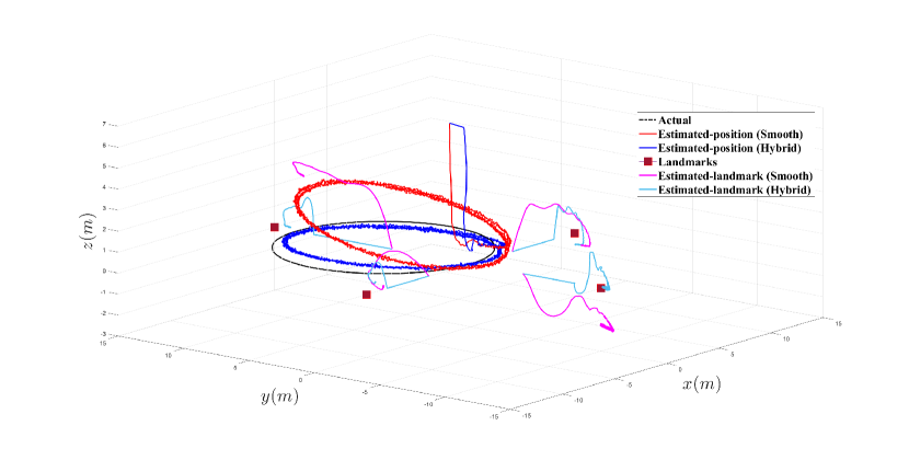
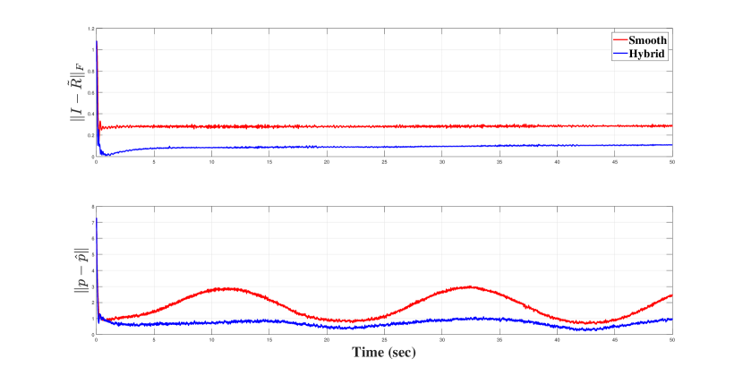
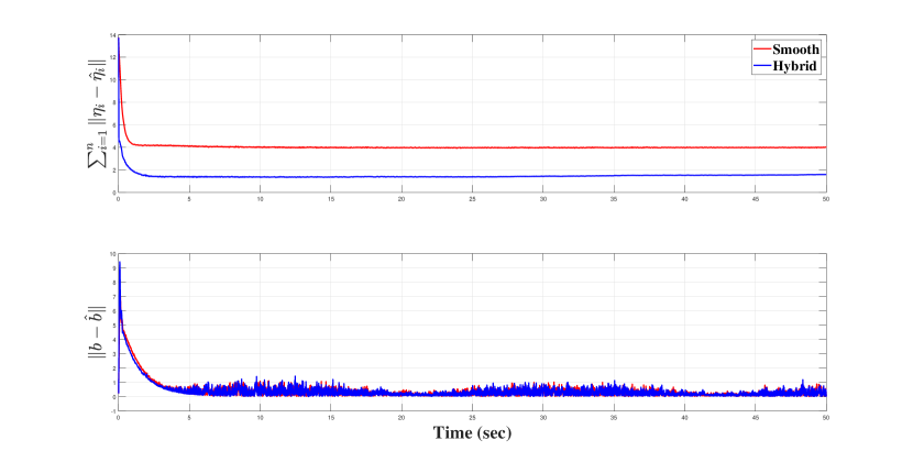
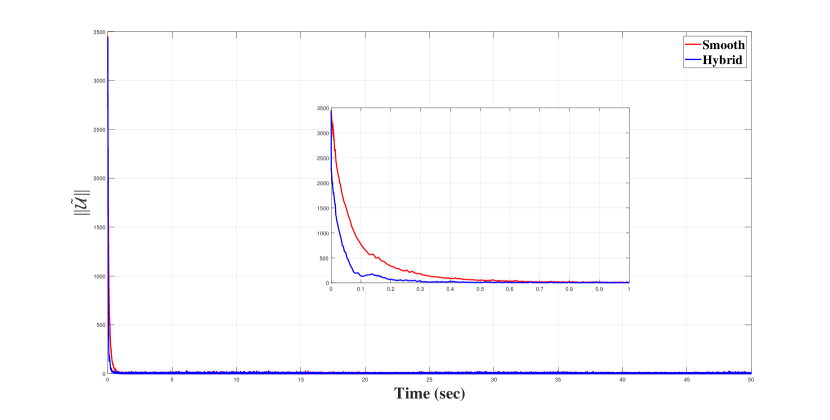
In this experiment, the robot moves in a circular trajectory at a constant altitude. The unbiased measurements of the angular velocity and linear velocity in the body-fixed frame are such that $\omega=[0\ 0\ 0.3]^{T}$ $rad/sec$ and $v=[2\ 0\ 0]^{T}$ $m/sec$. The robot’s initial position and attitude were set to $p(0)=[0\ 0\ 0]^{T}$ and $R(0)=\mathfrak{R}(0,e_{1})$, respectively. The initial conditions for both observers were set to $\hat{p}(0)=[-2\ 0\ 7]^{T}$, $\hat{R}(0)=\mathfrak{R}(\pi/4,e_{1})$, and $\hat{\eta}=0.4*\eta$. Figures (1-4) illustrate the results of this experiment. Figure (1) depicts the estimated paths of the robot’s position and the landmarks’ positions versus time, as well as the actual robot path and landmark positions. The evolution of the attitude tracking error and position tracking error are shown in Figure (2). Figure (3) shows the errors associated with estimates of landmark locations and biases. The evolution of the Lyapunov functions is shown in Figure (4). These figures demonstrate that the proposed hybrid observer has lower estimation errors than the smooth observer. Furthermore, the convergence rate of the proposed observer is faster than that of the smooth observer.

Figure 1: 3D trajectories of the observers compared to the actual system evolution in the first experiment.

Figure 2: Estimation errors of attitude and position in the first experiment.

Figure 3: Norms of the velocity bias estimation errors and landmark position estimation errors in the first experiment.

Figure 4: Evolution of the Lyapunov functions versus time in the first experiment.

IV-B Second Experiment

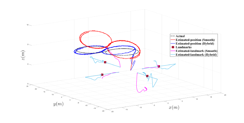
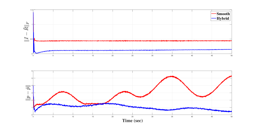
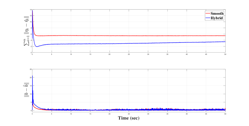
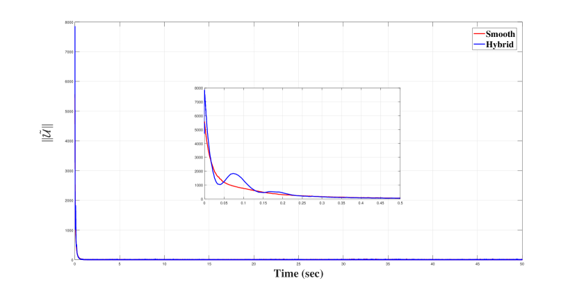
As discussed above, in this experiment, a different simulation scenario is used to further assess the performance of the proposed observer. The robot is simulated to move along a eight-shape trajectory at a fixed height of 4 $m$. The robot’s initial attitude and position were set to $R(0)=\mathfrak{R}(0,e_{1})$ and $p(0)=[0\ 0\ 4]^{T}$, respectively. In this experiment, angular velocity was assumed to be $\omega=[0\ 0\ \pm 0.4]^{T}$ $rad/sec$, and linear velocity was assumed to be $v=[2\ 0\ 0]^{T}$ $m/sec$. Both observers were initialized at $\hat{p}(0)=[0\ 0\ 0]^{T}$, $\hat{R}(0)=\mathfrak{R}(\pi/3,e_{1})$, and $\hat{\eta}=0.4*\eta$. The simulation results of the second experiment are shown in Figures (5-8). Figure (5) shows the 3D trajectories of the robot’s position tracking and estimated landmark locations, as well as the true robot trajectory and actual landmark locations. The errors in the estimation of attitude, robot path, landmark locations, and biases are illustrated in Figures (6,7). Figure (8) shows the evolution of the Lyapunov functions. These figures reveal that the proposed hybrid observer performs better than the smooth observer on both trajectory tracking and reducing the effect of noise.

Figure 5: 3D trajectories of the observers compared to actual system evolution in the second experiment.

Figure 6: Estimation errors of attitude and position in the second experiment.

Figure 7: Norms of the velocity bias estimation errors and landmark position estimation errors in the second experiment.

Figure 8: Evolution of the Lyapunov functions versus time in the second experiment.

V Conclusion

The present paper has investigated the problem of global convergence in SLAM observers. Most state-of-the-art SLAM techniques can guarantee almost global convergence due to the non-contractibility of the state-space of attitude. Accordingly, this paper has introduced a gradient-based hybrid observer to overcome topological obstructions and achieve global convergence. The proposed algorithm was demonstrated to be globally asymptotically convergent. Finally, the proposed hybrid observer was compared to a smooth observer, demonstrating the superior performance of the proposed algorithm.

Appendix A Some Useful Identities

This paper uses the following identities related to the orthogonal projection and matrix inner product.

$$\begin{split}&\Upsilon(\mathcal{X}B)=\Upsilon(\mathcal{X}^{-T}B),\quad(a)\\ &\left\langle\mathcal{V},B\right\rangle=\left\langle\mathcal{V},\Upsilon(B)\right\rangle=\left\langle\Upsilon(B),\mathcal{V}\right\rangle,\quad(b)\\ &\text{tr}(ABCD)=\text{tr}(CDAB)=\text{tr}(DABC),\quad(c)\\ \end{split}$$

References

- [1] P. Mäkinen, M. M. Aref, J. Mattila, and S. Launis, “Application of simultaneous localization and mapping for large-scale manipulators in unknown environments,” in 2019 IEEE International Conference on Cybernetics and Intelligent Systems (CIS) and IEEE Conference on Robotics, Automation and Mechatronics (RAM). IEEE, 2019, pp. 559–564.
- [2] T. Bailey and H. Durrant-Whyte, “Simultaneous localization and mapping (slam): Part ii,” IEEE robotics & automation magazine, vol. 13, no. 3, pp. 108–117, 2006.
- [3] J. A. Castellanos, J. Neira, and J. D. Tardós, “Limits to the consistency of ekf-based slam,” IFAC Proceedings Volumes, vol. 37, no. 8, pp. 716–721, 2004.
- [4] R. Mahony and T. Hamel, “A geometric nonlinear observer for simultaneous localisation and mapping,” in 2017 IEEE 56th Annual Conference on Decision and Control (CDC). IEEE, 2017, pp. 2408–2415.
- [5] S. Huang and G. Dissanayake, “Convergence and consistency analysis for extended kalman filter based slam,” IEEE Transactions on robotics, vol. 23, no. 5, pp. 1036–1049, 2007.
- [6] S. Hashemi and A. Alfi, “Doppler and bearing tracking using fuzzy adaptive unscented kalman filter,” Iranian Journal of Fuzzy Systems, vol. 16, no. 4, pp. 97–114, 2019.
- [7] S. H. Hashemi and A. Alfi, “Doppler and bearing tracking using adaptive modified covariance extended kalman filter,” Journal of Control, vol. 12, no. 4, pp. 23–33, 2019.
- [8] G. P. Huang, A. I. Mourikis, and S. I. Roumeliotis, “A quadratic-complexity observability-constrained unscented kalman filter for slam,” IEEE Transactions on Robotics, vol. 29, no. 5, pp. 1226–1243, 2013.
- [9] Y. Song, Z. Zhang, J. Wu, Y. Wang, L. Zhao, and S. Huang, “A right invariant extended kalman filter for object based slam,” IEEE Robotics and Automation Letters, 2021.
- [10] M. Tang, Z. Chen, and F. Yin, “Robot tracking in slam with masreliez-martin unscented kalman filter,” International Journal of Control, Automation and Systems, vol. 18, no. 9, pp. 2315–2325, 2020.
- [11] G. P. Huang, A. I. Mourikis, and S. I. Roumeliotis, “Analysis and improvement of the consistency of extended kalman filter based slam,” in 2008 IEEE International Conference on Robotics and Automation. IEEE, 2008, pp. 473–479.
- [12] H. He, K. Wang, and L. Sun, “A slam algorithm of fused ekf and particle filter,” in 2018 WRC Symposium on Advanced Robotics and Automation (WRC SARA). IEEE, 2018, pp. 172–177.
- [13] M. S. Bahraini, “On the efficiency of slam using adaptive unscented kalman filter,” Iranian Journal of Science and Technology, Transactions of Mechanical Engineering, vol. 44, no. 3, pp. 727–735, 2020.
- [14] R. Havangi, “Robust slam: Slam base on square root unscented kalman filter,” Nonlinear Dynamics, vol. 83, no. 1, pp. 767–779, 2016.
- [15] D. E. Zlotnik and J. R. Forbes, “Gradient-based observer for simultaneous localization and mapping,” IEEE Transactions on Automatic Control, vol. 63, no. 12, pp. 4338–4344, 2018.
- [16] M. Wang and A. Tayebi, “Geometric nonlinear observer design for slam on a matrix lie group,” in 2018 IEEE Conference on Decision and Control (CDC). IEEE, 2018, pp. 1488–1493.
- [17] H. A. Hashim and A. E. Eltoukhy, “Landmark and imu data fusion: Systematic convergence geometric nonlinear observer for slam and velocity bias,” IEEE Transactions on Intelligent Transportation Systems, 2020.
- [18] H. A. Hashim, “Guaranteed performance nonlinear observer for simultaneous localization and mapping,” IEEE Control Systems Letters, vol. 5, no. 1, pp. 91–96, 2020.
- [19] R. Mahony, T. Hamel, and J. Trumpf, “An homogeneous space geometry for simultaneous localisation and mapping,” Annual Reviews in Control, vol. 51, pp. 254–267, 2021.
- [20] P. van Goor, R. Mahony, T. Hamel, and J. Trumpf, “A geometric observer design for visual localisation and mapping,” in 2019 IEEE 58th Conference on Decision and Control (CDC). IEEE, 2019, pp. 2543–2549.
- [21] ——, “An observer design for visual simultaneous localisation and mapping with output equivariance,” IFAC-PapersOnLine, vol. 53, no. 2, pp. 9560–9565, 2020.
- [22] ——, “Constructive observer design for visual simultaneous localisation and mapping,” Automatica, vol. 132, p. 109803, 2021.
- [23] M. Wang and A. Tayebi, “Hybrid pose and velocity-bias estimation on se(3) using inertial and landmark measurements,” IEEE Transactions on Automatic Control, vol. 64, no. 8, pp. 3399–3406, 2018.
- [24] S. H. Hashemi, N. Pariz, and S. K. H. Sani, “Observer-based adaptive hybrid feedback for robust global attitude stabilization of a rigid body,” IEEE Transactions on Aerospace and Electronic Systems, vol. 57, no. 3, pp. 1919–1929, 2021.
- [25] S. H. Hashemi, N. Pariz, and S. K. Hosseini Sani, “Observer-based hybrid control for global attitude tracking on so(3) with input quantization,” International Journal of Control, no. just-accepted, p. 1, 2022.
- [26] M. Wang and A. Tayebi, “Globally asymptotically stable hybrid observers design on se(3),” in 2017 IEEE 56th Annual Conference on Decision and Control (CDC). IEEE, 2017, pp. 3033–3038.
- [27] ——, “A globally exponentially stable nonlinear hybrid observer for 3d inertial navigation,” in 2018 IEEE Conference on Decision and Control (CDC). IEEE, 2018, pp. 1367–1372.
- [28] ——, “Hybrid nonlinear observers for inertial navigation using landmark measurements,” IEEE Transactions on Automatic Control, vol. 65, no. 12, pp. 5173–5188, 2020.
- [29] ——, “Nonlinear state estimation for inertial navigation systems with intermittent measurements,” Automatica, vol. 122, p. 109244, 2020.
- [30] R. Goebel, R. G. Sanfelice, and A. R. Teel, “Hybrid dynamical systems,” IEEE Control Systems Magazine, vol. 29, no. 2, pp. 28–93, 2009.
- [31] A. R. Teel, F. Forni, and L. Zaccarian, “Lyapunov-based sufficient conditions for exponential stability in hybrid systems,” IEEE Transactions on Automatic Control, vol. 58, no. 6, pp. 1591–1596, 2012.
- [32] S. H. Hashemi, N. Pariz, and S. K. Hosseini Sani, “Global exponential stabilization of a quadrotor by hybrid control,” Transactions of the Institute of Measurement and Control, vol. 43, no. 10, pp. 2345–2357, 2021.
- [33] J.-C. Bourin, “Matrix versions of some classical inequalities,” Linear algebra and its applications, vol. 416, no. 2-3, pp. 890–907, 2006.