Compatible $L^{2}$ norm convergence of variable-step L1 scheme for the time-fractional MBE mobel with slope selection

Abstract

The convergence of variable-step L1 scheme is studied for the time-fractional molecular beam epitaxy (MBE) model with slope selection. A novel asymptotically compatible $L^{2}$ norm error estimate of the variable-step L1 scheme is established under a convergence-solvability-stability (CSS)-consistent time-step constraint. The CSS-consistent condition means that the maximum step-size limit required for convergence is of the same order to that for solvability and stability (in certain norms) as the small interface parameter $\epsilon\rightarrow 0^{+}$. To the best of our knowledge, it is the first time to establish such error estimate for nonlinear subdiffusion problems. The asymptotically compatible convergence means that the error estimate is compatible with that of backward Euler scheme for the classical MBE model as the fractional order $\alpha\rightarrow 1^{-}$. Just as the backward Euler scheme can maintain the physical properties of the MBE equation, the variable-step L1 scheme can also preserve the corresponding properties of the time-fractional MBE model, including the volume conservation, variational energy dissipation law and $L^{2}$ norm boundedness. Numerical experiments are presented to support our theoretical results.

Keywords:   time-fractional MBE equation with slope selection; variable-step L1 scheme; asymptotically compatible convergence; convergence-solvability-stability-consistent time-step condition; variational energy dissipation law
AMS subject classiffications.   35Q99, 65M06, 65M12, 74A50

1 Introduction

Consider the well-known Ehrlich–Schwoebel energy given as [14, 23]

$$E[\Phi]=\int_{\Omega}\frac{\epsilon^{2}}{2}|\Delta\Phi|^{2}+F(\nabla\Phi)\,\mathrm{d}{\mathbf{x}},$$ (1.1)

where the domain $\Omega=(0,L)^{2}\subset\mathbb{R}^{2}$, the constant $\epsilon>0$ represents the width of the rounded corners on the otherwise faceted crystalline thin films, $\Phi$ is a scaled height function of a thin film, and $F(\mathbf{v})=\frac{1}{4}(|\mathbf{v}|^{2}-1)^{2}$ is a nonlinear energy density function. The MBE model with slope selection can be viewed as the $L^{2}$ gradient flow associated with the free energy (1.1),

$$\partial_{t}\Phi:=-\kappa\mu\quad\text{with}\quad\mu:=\frac{\delta E}{\delta\Phi},$$ (1.2)

where $\mu$ is the vatiational derivative of the free energy $E$, $\kappa$ is a positive mobility constant, and the nonlinear vector functional $f(\mathbf{v})=F^{\prime}(\mathbf{v})=(|\mathbf{v}|^{2}-1)\mathbf{v}$. This model is widely used in material science because it can accurately capture the growth of high-quality crystalline materials [23]. Under periodic boundary conditions, it is easy to check that the MBE system (1.2) preserves the volume conservation $\big{(}\Phi(t),1\big{)}=\big{(}\Phi(0),1\big{)}$, the energy dissipation law

$$\frac{\,\mathrm{d}E}{\,\mathrm{d}t}+\kappa\big{\|}\mu\big{\|}_{L^{2}}^{2}=0,$$ (1.3)

and the following $L^{2}$ norm estimate, cf. the derivation of (1.9),

$$\left\|\Phi\right\|_{L^{2}}^{2}\leq\left\|\Phi_{0}\right\|_{L^{2}}^{2}+\frac{\kappa}{2}\left|\Omega\right|t,$$ (1.4)

where $(\cdot,\cdot)$ and $\left\|\cdot\right\|_{L^{2}}$ hongare the usual inner product and the associated $L^{2}$ norm.

Recently, many researchers paid great attention to the time fractional phase field models [5, 12, 7, 3, 29, 2] to accurately describe the long time memory and the anomalously diffusive effects. In this paper, we aim to develop a reliable numerical scheme for the time-fractional molecular beam epitaxy (TFMBE) model with slope selection, see [5, 29],

$$\partial^{\alpha}_{t}\Phi=-\kappa\mu\quad\text{with}\quad\mu=\epsilon^{2}\Delta^{2}\Phi-\nabla\cdot f(\nabla\Phi),$$ (1.5)

subject to the periodic boundary condition and initial condition $\Phi(\mathbf{x},0):=\Phi_{0}(\mathbf{x})$. As shown latter, this TFMBE model (1.5) also retains some of continuous properties of the classical MBE model (1.2). Here, $\partial^{\alpha}_{t}:={{}^{C}_{0}\mathcal{D}^{\alpha}_{t}}$ is the Caputo derivative of order $\alpha$,

$${\partial^{\alpha}_{t}v}={{}^{C}_{0}\mathcal{D}^{\alpha}_{t}v}:=\mathcal{I}^{1-\alpha}_{t}v^{\prime}\quad\text{for $0<\alpha<1$,}$$

where $\mathcal{I}^{\beta}_{t}$ is the fractional Riemann–Liouville integral operator of order $\beta>0$,

$$(\mathcal{I}^{\beta}_{t}v)(t):=\int_{0}^{t}\omega_{\beta}(t-s)v(s)\,\mathrm{d}{s}\quad\text{with $\omega_{\beta}(t):=\frac{t^{\beta-1}}{\Gamma(\beta)}$}.$$

1.1 Continuous properties

We describe some continuous properties of the TFMBE model (1.5), which are natural extensions of the physical properties of (1.2), including the volume conservation, energy dissipation law (1.3) and $L^{2}$ norm stability (1.4).

Tang, Yu and Zhou [29] have established the volume conservation $\big{(}\Phi(t),1\big{)}=\big{(}\Phi(0),1\big{)}$ and the following global energy dissipation law

$$E[\Phi(t)]\leq E[\Phi(0)]\quad\text{for $t>0$},$$

which is quite different from the local energy decaying property (1.3). In order to be compatible with the classical model, we consider a variational energy functional in [20],

$$\mathcal{E}_{\alpha}[\Phi]:=E[\Phi]+\frac{\kappa}{2}\mathcal{I}_{t}^{\alpha}\big{\|}\mu\big{\|}_{L^{2}}^{2}\quad\text{for $t>0$}.$$ (1.6)

Obviously, this variational energy functional admits a local energy dissipation law

$$\frac{\,\mathrm{d}\mathcal{E}_{\alpha}}{\,\mathrm{d}t}+\frac{\kappa}{2}\omega_{\alpha}(t)\big{\|}\mu\big{\|}_{L^{2}}^{2}\leq 0.$$ (1.7)

This type energy functional $\mathcal{E}_{\alpha}[\Phi]$ is introduced firstly by Liao et al [20] in exploring the L1-type formula of Riemann–Liouville derivative for the time-fractional Allen–Cahn equation. If the fractional order $\alpha\rightarrow 1^{-}$, the local energy decaying law (1.7) asymptotically recovers the classical energy dissipation law in the form of

$$\frac{\,\mathrm{d}E}{\,\mathrm{d}t}+\kappa\left\|\mu\right\|_{L^{2}}^{2}\leq 0.$$

In addition, by taking the $L^{2}$ inner product of the TFMBE model (1.5) with $\Phi$, and using the Green’s formula, one gets

$$\left(\partial^{\alpha}_{t}\Phi,\Phi\right)+\kappa\epsilon^{2}\left\|\Delta\Phi\right\|_{L^{2}}^{2}-\kappa\left(f(\nabla\Phi),\nabla\Phi\right)=0.$$ (1.8)

For the nonlinear term, one has

$$\left(f(\mathbf{v}),\mathbf{v}\right)=\left((|\mathbf{v}|^{2}-\tfrac{1}{2})^{2}-\tfrac{1}{4},1\right)\geq-\frac{1}{4}\left(1,1\right)=-\frac{1}{4}\left|\Omega\right|.$$

By inserting it into (1.8) and using the inequality $\left(\partial_{t}^{\alpha}\Phi,\Phi\right)\geq\frac{1}{2}\partial_{t}^{\alpha}\left\|\Phi\right\|_{L^{2}}^{2}$ from [1, Lemma 2], one can reformulate the equation (1.8) into the following form

$$\partial_{t}^{\alpha}\left\|\Phi\right\|_{L^{2}}^{2}\leq\frac{\kappa}{2}\left|\Omega\right|,\quad t>0.$$

By acting the Riemann-Liouville integral operator $\mathcal{I}^{\alpha}_{t}$ on both sides, one has

$$\left\|\Phi\right\|_{L^{2}}^{2}\leq\left\|\Phi_{0}\right\|_{L^{2}}^{2}+\frac{\kappa}{2}\left|\Omega\right|\omega_{1+\alpha}(t),\quad t>0.$$ (1.9)

It is seen that, in the fractional order limit $\alpha\rightarrow 1^{-}$, the $L^{2}$ norm stability estimate (1.9) is asymptotically compatible with (1.4) of the classical MBE equation (1.2).

1.2 Our contribution

Some numerical methods were also proposed recently in [5, 12, 29] for the TFMBE equation. The numerical scheme in [5] utilized the fast L1 algorithm for the Caputo derivative, but the $2-\alpha$ order of convergence was verified only experimentally. Ji et al. [12] suggested a variable-step L$1^{+}$ scheme for the Caputo derivative with second-order accuracy, and developed two Crank-Nicolson-type methods based on the energy quadratization strategy. However, due to the lack of solution estimate, no convergence results are available in the literature for the numerical solutions of the TFMBE equation (1.5). In this paper, a rigorous $L^{2}$ norm convergence analysis is presented for the variable-step L1 scheme. This scheme is asymptotically compatible with the backward Euler scheme for the classical MBE model (1.2) as the fractional order $\alpha\rightarrow 1^{-}$. Just as the backward Euler scheme can maintain the physical properties of the MBE equation, the variable-step L1 scheme can also preserve the corresponding properties of the time-fractional MBE model, including the volume conservation, varitional energy dissipation law (1.7) and $L^{2}$ norm stability (1.9) at the discrete levels.

Table 1: The CSS-consistent time-step conditions.

	variable-step L1 scheme	backward Euler scheme ($\alpha\rightarrow 1^{-}$)
Convergence	$\tau_{n}\leq\sqrt[\alpha]{2\omega_{2-\alpha}(1)\epsilon^{2}/\kappa}$	$\tau_{n}\leq 2\epsilon^{2}/\kappa$
Solvability	$\tau_{n}\leq\sqrt[\alpha]{4\omega_{2-\alpha}(1)\epsilon^{2}/\kappa}$	$\tau_{n}\leq 4\epsilon^{2}/\kappa$
Energy stability	$\tau_{n}\leq\sqrt[\alpha]{4\omega_{2-\alpha}(1)\epsilon^{2}/\kappa}$	$\tau_{n}\leq 4\epsilon^{2}/\kappa$
$L^{2}$ norm stability	$\tau_{n}=O\left(1\right)$	$\tau_{n}=O\left(1\right)$

Many effective numerical methods [8, 4, 9, 10, 11, 24, 26, 27, 30, 32], including convex splitting methods, stabilized semi-implicit methods, exponential time differencing approaches and energy quadratization methods, have been explored rigorously for nonlinear phase field equations including the MBE model. However, compared with the somewhat weak (or no) time-step constraints for solvability or the energy dissipation law, the associated convergence analyses always suffer from very severe step-size restrictions with respect to the small interface parameter $\epsilon$ in the existing works. For example, the stablized method in [9] is unconditional energy stable with the step-size $\tau=O(1)$, but the convergence requires very small time-steps, nearly $\tau=O(\epsilon^{14})$. It is an obvious defect at least in theoretical manner. By making full use of the convexity of nonlinear functional $f(\mathbf{v})$, we establish an asymptotically compatible $L^{2}$ norm error estimate of the variable-step L1 scheme under a convergence-solvability-stability (CSS)-consistent time-step constraint. The CSS-consistent condition means that the maximum step-size limit required for convergence is of the same order to that for solvability and stability as the small interface parameter $\epsilon\rightarrow 0^{+}$. To the best of our knowledge, it is the first time to establish such error estimate for nonlinear subdiffusion problems. Also, the imposed CSS-consistent time-step condition is asymptotically compatible with the time-step constraint of the backward Euler scheme as the fractional order $\alpha\rightarrow 1^{-}$, see Table 1.

In summary, our contribution is three-fold:

• By making use of the convexity of nonlinear bulk, a rigorous $L^{2}$ norm error estimate of the varaibel-step L1 scheme is established, maybe at the first time, under a CSS-consistent time-step condition. This estimate is robust and asymptotically compatible with that of the backward Euler scheme for the classical MBE model as $\alpha\rightarrow 1^{-}$.

• The variable step L1 scheme is proven to preserve the volume conservation, the variational energy dissipation law and $L^{2}$ norm stability so that it is practically reliable in long-time simulations.

• Several numerical examples are included to show the accuracy and effectiveness of the variable-step L1 scheme with an adaptive time-stepping strategy.

The rest of the paper is organized as follows. Next section presents the nonuniform L1 implicit scheme and the unique solvability. The asymptotically compatible $L^{2}$ norm convergence is established in section 3. Section 4 addresses the discrete counterparts of the varitional energy dissipation law (1.7) and $L^{2}$ norm stability (1.9) at the discrete levels. Some numerical examples are included in the last section.

2 The variable-step L1 scheme and solvability

2.1 Nonuniform L1 formula

The TFMBE model (1.5) has multi-scale behavior in a rough-smooth-rough pattern, especially at an early stage of epitaxial growth on rough surfaces. It is practically useful to adopt some adaptive time-stepping strategy in the coarsening dynamics approaching the steady state. It is desirable to investigate the time approximation on a general class of time meshes.

Consider $0=t_{0}<\cdots<t_{k-1}<t_{k}<\cdots<t_{N}=T$ for a finite $T>0$. Let the variable time-steps $\tau_{k}:=t_{k}-t_{k-1}$ for $1\leq k\leq N$. We use the maximum step size $\tau:=\max_{1\leq k\leq N}\tau_{k}$, and the adjoint time-step ratios $r_{k}:=\tau_{k}/\tau_{k-1}$ for $2\leq k\leq N$. Given a grid function $\{v_{k}\}^{N}_{k=0}$, let $\triangledown_{\tau}v^{k}=v^{k}-v^{k-1}$ and $\partial_{\tau}v^{k}:=\triangledown_{\tau}v^{k}/\tau_{k}$ for $k\geq 1$. The nonuniform L1 formula of Caputo derivative reads, see [16, 17],

$$\left(\partial_{\tau}^{\alpha}v\right)^{n}:=\sum_{k=1}^{n}a_{n-k}^{(n)}\triangledown_{\!\tau}v^{k}\quad\text{for $n\geq 1$,}$$ (2.1)

where the discrete coefficients $a_{n-k}^{(n)}$ are defined by

$$a_{n-k}^{(n)}:=\frac{1}{\tau_{k}}\int_{t_{k-1}}^{t_{k}}\omega_{1-\alpha}(t_{n}-s)\,\mathrm{d}{s}\quad\text{for $1\leq{k}\leq{n}$}.$$ (2.2)

We know that the discrete L1 kernels $a_{n-k}^{(n)}$ are positive and monotone on arbitrary time meshes [18, 21]. To deal with the discrete kernels, we introduce two important discrete tools, namely discrete orthogonal convolution (DOC) kernels and discrete complementary convolution (DCC) kernels. The DOC kernels $\theta^{(n)}_{n-k}$ are defined via a recursive procedure [19]

$${\theta_{0}^{(n)}}:=\frac{1}{a_{0}^{(n)}}\quad\text{and}\quad{\theta_{n-k}^{(n)}}:=-\frac{1}{a_{0}^{(k)}}\sum^{n}_{j=k+1}{\theta_{n-j}^{(n)}}a^{(j)}_{j-k}\quad\text{for $1\leq k\leq n-1$}.$$ (2.3)

There has the following discrete orthogonal identity

$$\sum_{j=k}^{n}\theta_{n-j}^{(n)}a_{j-k}^{(j)}\equiv\delta_{nk}\quad\text{for $1\leq k\leq n$},$$ (2.4)

where $\delta_{nk}$ is the Kronecker delta symbol. The DCC kernels are defined as [18]

$${p^{(n)}_{n-k}}:=\sum^{n}_{j=k}{\theta_{j-k}^{(j)}}\quad\text{for $1\leq k\leq n$}.$$ (2.5)

As proven in [18, Subsection 2.2], the discrete convolution kernels ${p^{(n)}_{n-k}}$ are complementary to the discrete L1 kernels $a_{n-k}^{(n)}$ in the following sense,

$$\sum^{n}_{j=k}{p^{(n)}_{n-j}}a_{j-k}^{(j)}\equiv 1\quad\text{for $1\leq k\leq n$}.$$ (2.6)

Figure 1 describes the above connections among three types of discrete convolution kernels.

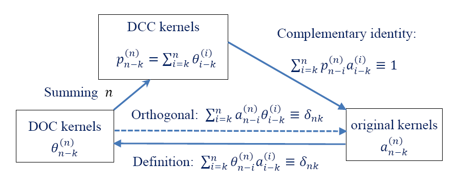
Figure 1: The relationship diagram of DOC and DCC kernels

In the following convergence and stability analysis, we need the following result.

Lemma 2.1

[16, Lemma 2.1] For any $n\geq 2$, the DCC kernels $p_{n-k}^{(n)}$ in (2.5) satisfy,

$$p_{n-k}^{(n)}\geq 0\quad\text{for $1\leq k\leq n$},\quad\text{and}\quad\sum_{j=1}^{n}p_{n-j}^{(n)}\leq\omega_{1+\alpha}(t_{n}).$$

2.2 Fully discrete scheme

Fourier pseudo-spectral method in space is adopted here. Consider the discrete spatial grid $\bar{\Omega}_{h}:=\{\mathbf{x}_{h}=(ih,jh)~{}|~{}0\leq i,j\leq M\}$ and $\Omega_{h}:=\bar{\Omega}_{h}\cap\Omega$, where $M$ is an even positive integer and the uniform length $h:=L/M$. Let $\mathscr{F}_{M}$ be the trigonometric polynomials space (all trigonometric polynomials of degree up to $M/2$). Let $P_{M}:L^{2}(\Omega)\rightarrow\mathscr{F}_{M}$ and $I_{M}:L^{2}(\Omega)\rightarrow\mathscr{F}_{M}$ be the $L^{2}$-projection operator and the trigonometric interpolation operator of the periodic function $v(\mathbf{x})\in L^{2}(\Omega)$, respectively, that is,

$$(P_{M}v)(\mathbf{x})=\sum_{m,n=-M/2}^{M/2-1}\hat{v}_{m,n}e_{m,n}(\mathbf{x}),\quad(I_{M}v)(\mathbf{x})=\sum_{m,n=-M/2}^{M/2-1}\tilde{v}_{m,n}e_{m,n}(\mathbf{x}),$$

where the basis function $e_{m,n}(\mathbf{x}):=e^{i\nu\left(mx+ny\right)}$ with $\nu=2\pi/L$, the coefficients $\hat{v}_{m,n}$ denote the standard Fourier coefficients of $v(\mathbf{x})$, and the pseudo-spectral coefficients $\tilde{v}_{m,n}$ are determined such that $(I_{M}v)(\mathbf{x}_{h})=v(\mathbf{x}_{h})$. In turn, the Fourier pseudo-spectral first- and second-order derivatives of $v_{h}$ are given by

$$\mathcal{D}_{x}v_{h}:=\sum_{m,n=-M/2}^{M/2-1}(i\nu m)\tilde{v}_{m,n}e_{m,n}(\mathbf{x}),\quad\mathcal{D}_{x}^{2}v_{h}:=\sum_{m,n=-M/2}^{M/2-1}(i\nu m)\tilde{v}_{m,n}e_{m,n}(\mathbf{x}).$$

The notations $\mathcal{D}_{y}$ and $\mathcal{D}_{y}^{2}$ would be defined silimarly. Accordingly, the discrete gradient $\nabla_{h}$ and Laplacian $\Delta_{h}$ in the point-wise sense are given by

$$\nabla_{h}v_{h}:=(\mathcal{D}_{x}v_{h},\mathcal{D}_{y}v_{h})^{T}\quad\text{and}\quad\Delta_{h}v_{h}:=(\mathcal{D}^{2}_{x}v_{h},\mathcal{D}^{2}_{y}v_{h}).$$

In the numerical analysis, let $\mathbb{V}_{h}:=\{v\,|\,v=\left(v_{h}\right)\;\text{is L-periodic for}\;\mathbf{x}_{h}\in\bar{\Omega}_{h}\}$ be the space of L-periodic grid functions. For any functions $v,w\in\mathbb{V}_{h}$, the following discrete Green’s formulas hold $\left\langle-\Delta_{h}v,w\right\rangle=\left\langle\nabla_{h}v,\nabla_{h}w\right\rangle$ and $\left\langle\Delta^{2}_{h}v,w\right\rangle=\left\langle\Delta_{h}v,\Delta_{h}w\right\rangle$. Also, we define the discrete inner product $\left\langle v,w\right\rangle:=h^{2}\sum_{\mathbf{x}_{h}\in\Omega_{h}}v_{h}w_{h}$, the associated $L^{2}$ norm $\left\|v\right\|:=\sqrt{\left\langle v,v\right\rangle}$ and the discrete $L^{p}$ norm $\left\|v\right\|_{l^{p}}:=\sqrt[p]{h^{2}\sum_{\mathbf{x}_{h}\in\Omega_{h}}\left|v_{h}\right|^{p}}$ for any grid functions $v,w\in\mathbb{V}_{h}$. The discrete $H^{1}$ and $H^{2}$ norms are defined as

$$\left\|v\right\|^{2}_{H_{h}^{1}}:=\left\|v\right\|^{2}+\left\|\nabla_{h}v\right\|^{2},\quad\left\|v\right\|^{2}_{H_{h}^{2}}:=\left\|v\right\|^{2}_{H_{h}^{1}}+\left\|\Delta_{h}v\right\|^{2}.$$

We compute the numerical solution $\phi_{h}^{n}\in\mathbb{V}_{h}$ of the TFMBE model (1.5) by the fully implicit time-stepping scheme

$$\left(\partial_{\tau}^{\alpha}\phi_{h}\right)^{n}=-\kappa\mu_{h}^{n}\quad\text{with}\quad\mu_{h}^{n}=\epsilon^{2}\Delta_{h}^{2}\phi_{h}^{n}-\nabla_{h}\cdot f\left(\nabla_{h}\phi_{h}^{n}\right),$$ (2.7)

with the initial data $\phi_{h}^{0}=(P_{M}\Phi_{0})(\mathbf{x}_{h})$ for $\mathbf{x}_{h}\in\Omega_{h}$. In order to facilitate our comparisons, we also describe the backward Euler scheme for the calssical MBE model (1.2),

$$\partial_{\tau}\phi_{h}^{n}=-\kappa\mu_{h}^{n}\quad\text{with}\quad\mu_{h}^{n}=\epsilon^{2}\Delta_{h}^{2}\phi_{h}^{n}-\nabla_{h}\cdot f\left(\nabla_{h}\phi_{h}^{n}\right).$$ (2.8)

It is not difficult to check that, if the time-step size $\tau_{n}\leq{4\epsilon^{2}}/{\kappa}$, the backward Euler scheme (2.8) is uniquely solvable and fulfills the following energy dissipation law [33]

$$\partial_{\tau}E[\phi^{n}]+\frac{\kappa}{2}\left\|\mu^{n}\right\|^{2}\leq 0.$$ (2.9)

When the fractional index $\alpha\rightarrow 1^{-}$, the discrete L1 kernels in (2.2) satisfy $a_{0}^{(n)}\rightarrow 1/\tau_{n}$ and $a_{n-k}^{(n)}\rightarrow 0$ for $1\leq k\leq n-1$. Then, $\left(\partial_{\tau}^{\alpha}\phi_{h}\right)^{n}\rightarrow\partial_{\tau}\phi_{h}^{n}$ as $\alpha\rightarrow 1^{-}$. The nonuniform L1 scheme (2.7) is asymptotically compatible with the backward Euler scheme (2.8) in the fractional order limit $\alpha\rightarrow 1^{-}$.

2.3 Unique solvability

The full discrete scheme (2.7) is volume conservative and unique solvable.

Lemma 2.2

The full discrete scheme (2.7) satisfies $\big{\langle}\phi^{k},1\big{\rangle}=\big{\langle}\phi^{0},1\big{\rangle}$ for $1\leq k\leq N$.

Proof  The discrete Green’s formula gives $\big{\langle}\mu^{n},1\big{\rangle}=0$ from the second equation of (2.7). Thus the first equation of (2.7) yields $0=\big{\langle}\left(\partial_{\tau}^{\alpha}\phi\right)^{k},1\big{\rangle}$ for $k\geq 1$. Multiplying both sides of the above equality by the DOC kernels $\theta_{n-k}^{(n)}$ and summing $k$ from $k=1$ to $n$, we have

$$0=\Big{\langle}\sum_{k=1}^{n}\theta_{n-k}^{(n)}\sum_{j=1}^{k}a_{k-j}^{(k)}\triangledown_{\!\tau}\phi^{j},1\Big{\rangle}=\big{\langle}\triangledown_{\!\tau}\phi^{n},1\big{\rangle}\quad\text{for $n\geq 1$,}$$

where the summation order was exchanged and the discrete orthogonal identity (2.4) was applied in the second equality. It gives $\left\langle\phi^{n},1\right\rangle=\left\langle\phi^{n-1},1\right\rangle$ and completes the proof.   

Theorem 2.1

If the time-step size satisfies

$$\tau_{n}\leq\sqrt[\alpha]{4\omega_{2-\alpha}(1)\epsilon^{2}/\kappa},$$ (2.10)

the nonuniform L1 scheme (2.7) is uniquely solvable.

Proof  We use the minimum principle of convex functional with a subspace of $\mathbb{V}_{h}$, that is, $\mathbb{V}^{*}_{h}:=\big{\{}z\in\mathbb{V}_{h}\,|\,\big{\langle}z,1\big{\rangle}=\big{\langle}\phi^{n-1},1\big{\rangle}\big{\}}$. Consider a discrete functional $G[z]$ on the space $\mathbb{V}^{*}_{h}$,

$$G[z]:=\frac{a_{0}^{(n)}}{2}\left\|z-\phi^{n-1}\right\|^{2}+\big{\langle}\mathcal{L}^{n-1},z-\phi^{n-1}\big{\rangle}+\frac{\epsilon^{2}\kappa}{2}\left\|\Delta_{h}z\right\|^{2}+\frac{\kappa}{4}\left\|\nabla_{h}z\right\|_{l^{4}}^{4}-\frac{\kappa}{2}\left\|\nabla_{h}z\right\|^{2},$$

where $n\geq 1$ and $\mathcal{L}^{n-1}:=\sum_{k=1}^{n-1}a_{n-k}^{(n)}\triangledown_{\!\tau}\phi^{k}.$ This functional $G[z]$ is strictly convex under the time-step condition (2.10) or $a_{0}^{(n)}\geq\kappa/(4\epsilon^{2})$. In fact, for any $\psi_{h}\in\mathbb{V}^{*}_{h}$,

$$\left.\frac{\,\mathrm{d}^{2}G}{\,\mathrm{d}s^{2}}[z+s\psi]\right|_{s=0} =a_{0}^{(n)}\left\|\psi\right\|^{2}+\epsilon^{2}\kappa\left\|\Delta_{h}\psi\right\|^{2}+3\kappa\left\|\nabla_{h}z\cdot\nabla_{h}\psi\right\|^{2}-\kappa\left\|\nabla_{h}\psi\right\|^{2}$$

$$\geq a_{0}^{(n)}\left\|\psi\right\|^{2}+\epsilon^{2}\kappa\left\|\Delta_{h}\psi\right\|^{2}+\kappa\big{\langle}\psi,\Delta_{h}\psi\big{\rangle}$$

$$\geq\big{(}a_{0}^{(n)}-\frac{\kappa}{4\epsilon^{2}}\big{)}\left\|\psi\right\|^{2}\geq 0,$$

where the Cauchy–Schwarz inequality and Young’s inequality have been used in third step. Next, we show that the functional $G[z]$ is coercive on $\mathbb{V}^{*}_{h}$,

$$G[z] \geq\frac{a_{0}^{(n)}}{2}\left\|z-\phi^{n-1}\right\|^{2}+\left\langle\mathcal{L}^{n-1},z-\phi^{n-1}\right\rangle+\frac{\kappa}{4}\left\|\nabla_{h}z\right\|_{l^{4}}^{4}-\frac{\kappa}{2}\left\|\nabla_{h}z\right\|^{2}$$

$$\geq\kappa\left\|\nabla_{h}z\right\|^{2}-\frac{1}{2a_{0}^{(n)}}\left\|\mathcal{L}^{n-1}\right\|^{2}-\frac{9\kappa}{4}\left|\Omega_{h}\right|,$$

where the inequality $\left\|\nabla_{h}z\right\|_{l^{4}}^{4}\geq 6\left\|\nabla_{h}z\right\|^{2}-9\left|\Omega_{h}\right|$, due to the fact $\big{\langle}(|\nabla_{h}z|^{2}-3)^{2},1\big{\rangle}\geq 0$, was used in the last step. Thus the functional $G[z]$ exists a unique minimizer, denote by $\phi_{h}^{n}$, if and only if it solves the following equation

$$\left.\frac{\,\mathrm{d}G}{\,\mathrm{d}s}[z+s\psi]\right|_{s=0}=\Big{\langle}a_{0}^{(n)}(z-\phi^{n-1})+\sum_{k=1}^{n-1}a^{(n)}_{n-k}\triangledown_{\!\tau}\phi^{k}+\kappa\epsilon^{2}\Delta_{h}z-\kappa\nabla_{h}\cdot f(\nabla_{h}z),\psi\Big{\rangle}=0.$$

This equation holds for any $\psi_{h}\in\mathbb{V}^{*}_{h}$ if and only if the unique minimizer $\phi_{h}^{n}\in\mathbb{V}^{*}_{h}$ solves

$$a_{0}^{(n)}(\phi_{h}^{n}-\phi_{h}^{n-1})+\sum_{k=1}^{n-1}a^{(n)}_{n-k}\triangledown_{\!\tau}\phi_{h}^{k}+\kappa\epsilon^{2}\Delta_{h}\phi_{h}^{n}-\kappa\nabla_{h}\cdot f(\nabla_{h}\phi_{h}^{n})=0,$$

which is just the scheme (2.7). The proof is completed.   

Note that, the time-step restriction (2.10) of solvability is sharp in the sense that it is compatible with that of the backward Euler scheme (2.8), that is,

$$\tau_{n}\leq\sqrt[\alpha]{4\omega_{2-\alpha}(1)\epsilon^{2}/\kappa}\quad\longrightarrow\quad\tau_{n}\leq 4\epsilon^{2}/\kappa\qquad\text{as $\alpha\rightarrow 1^{-}$}.$$

3 $L^{2}$ norm error estimate

This section presents the rigorous convergence analysis in the $L^{2}$ norm. We use the standard semi-norms and norms of the Sobolev space $H^{m}(\Omega)$. Let $\mathcal{C}_{per}^{\infty}(\Omega)$ be a set of infinitely differentiable $L$-periodic functions defined on $\Omega$, and $H_{per}^{m}(\Omega)$ be the closure of $\mathcal{C}_{per}^{\infty}(\Omega)$ in $H^{m}(\Omega)$, endowed with the semi-norm $\left|\cdot\right|_{H_{per}^{m}}$ and the norm $\left\|\cdot\right\|_{H_{per}^{m}}.$ For the simplicity of notation, we denote $\left|\cdot\right|_{H^{m}}:=\left|\cdot\right|_{H_{per}^{m}}$, $\left\|\cdot\right\|_{H^{m}}:=\left\|\cdot\right\|_{H_{per}^{m}}$, and $\left\|\cdot\right\|_{L^{2}}:=\left\|\cdot\right\|_{H^{0}}$.

We recall the $L^{2}$-projection operator $P_{M}$ and interpolation operator $I_{M}$ defined in Section 2, and denote the $L^{2}$-projection of exact solution $\Phi_{M}:=P_{M}\Phi$. The following lemma lists the projection error $P_{M}v-v$, and the interpolation error $I_{M}v-v$ in Sobolev space.

Lemma 3.1

[25] For any $v\in H^{q}_{per}(\Omega)$ and $0\leq s\leq q$, it holds that

$$\left\|P_{M}v-v\right\|_{H^{s}}\leq Ch^{q-s}\left|v\right|_{H^{q}},\quad\left\|P_{M}v\right\|_{H^{s}}\leq C\left\|v\right\|_{H^{s}};$$

and, in addition if $q>1,$

$$\left\|I_{M}v-v\right\|_{H^{s}}\leq Ch^{q-s}\left|v\right|_{H^{q}},\quad\left\|I_{M}v\right\|_{H^{s}}\leq C\left\|v\right\|_{H^{s}}.$$

3.1 Global consistency error

Numerical tests in [12] show that the TFMBE equation (1.5) admits a weak singularity near the initial time, like $\partial_{t}\Phi=O(t^{\alpha-1})$. To complete the convergence analysis on nonuniform time meshes, it is reasonable to assume that,

$$\big{\|}\Phi\big{\|}_{H^{m+4}}\leq C_{\phi},\quad\big{\|}\partial_{t}^{\alpha}\Phi\big{\|}_{H^{m}}\leq C_{\phi}\quad\text{and}\quad\big{\|}\partial_{t}^{(l)}\Phi\big{\|}_{H^{m}}\leq C_{\phi}(1+t^{\alpha-l}),$$ (3.1)

for $0<t\leq T$ and $l=1,2$, where $m\geq 0$ is an integer, $C_{\phi}$ denotes a generic positive constant. Such a regularity assumption on the exact solution of time-fractional phase field models with the Caputo time derivative is standard in the numerical analysis[7, 28, 3, 22, 13].

The analytical solution of the TFMBE equation (1.5) is weak singular at the initial time but regular away from the initial time. We put a grading parameter $\gamma\geq 1$ and assume that

1. there exists a constant $C_{\gamma}$, independent on the mesh, satisfies that the time-step sizes $\tau_{k}\leq\tau\min\{1,C_{\gamma}t_{k}^{1-1/\gamma}\}$ for $1\leq k\leq N$ and $t_{k}\leq C_{\gamma}t_{k-1}$ for $2\leq k\leq N$.

If the parameter $\gamma=1$, that means the mesh is quasi-uniform. As $\gamma$ increases, the initial step sizes are graded-like and become smaller compared to the others. On the other side, the assumption AG restricts only the maximum step size for the time mesh away from the initial time, so that the step sizes can be adjusted according to the solution behaviors. This point is very important in simulating the TFMBE model (1.5) because it admits complex multi-scale behaviors in the long-time coarsening dynamics, cf. Figures 2 and 4 in Section 5.

Let $\Upsilon^{j}=(\partial^{\alpha}_{t}v)(t_{j})-(\partial_{\tau}^{\alpha}v)^{j}$ denote the local consistency error of the variable-step L1 formula (2.1) at the time $t=t_{j}$. We have the following results for the global convolution approximation error $\sum_{j=1}^{n}p_{n-j}^{(n)}|\Upsilon^{j}|$, see [17, Lemma 3.1 and Lemma 3.3].

Lemma 3.2

[17, Lemma 3.1] For $v\in C^{2}(0,T]$ with $\int_{0}^{T}t|v_{tt}|\,\mathrm{d}t<\infty$, the global consistency error of the L1 formula (2.1) is bounded by

$$\sum_{j=1}^{n}p_{n-j}^{(n)}|\Upsilon^{j}|\leq 2\sum_{k=1}^{n}p_{n-k}^{(n)}a_{0}^{(k)}\int^{t_{k}}_{t_{k-1}}(t-t_{k-1})|v_{tt}|\,\mathrm{d}t.$$

We note that, the error bound in Lemma 3.2 is valid on arbitrary time meshes and is asymptotically compatible with the (global) truncation error of the backward Euler scheme (2.8). Actually, one has

$$\sum_{k=1}^{n}p_{n-k}^{(n)}a_{0}^{(k)}\int^{t_{k}}_{t_{k-1}}(t-t_{k-1})|v_{tt}|\,\mathrm{d}t\quad\longrightarrow\quad\sum_{k=1}^{n}\int^{t_{k}}_{t_{k-1}}(t-t_{k-1})|v_{tt}|\,\mathrm{d}t\quad\text{as $\alpha\rightarrow 1^{-}$.}$$

As desired, the limit is of temporal order $O(\tau)$. On the other hand, the error bound in the next Lemma is not asymptotically compatible in the fractional order limit $\alpha\rightarrow 1^{\color[rgb]{1,0,0}-}$. This defect is mainly due to the lack of some proper estimates for the DCC kernels $p_{n-k}^{(n)}$; however, it remains open to us up to now.

Lemma 3.3

[17, Lemma 3.3] If $v$ satisfies (3.1) and the meshes satisfy the assumption $\mathbf{AG}$, then the global consistency error of the L1 formula (2.1) can be bounded by

$$\sum_{j=1}^{n}p_{n-j}^{(n)}|\Upsilon^{j}|\leq\frac{C_{v}}{\alpha(1-\alpha)}\tau^{\min\{2-\alpha,\gamma\alpha\}}~{}~{}\text{for}~{}~{}1\leq n\leq N.$$

3.2 $L^{2}$ norm error estimate

We are in a position to present the $L^{2}$ norm error estimate for the variable-step L1 scheme (2.7). The involving notation $E_{\alpha}(z):=\sum_{k=0}^{\infty}\frac{z^{k}}{\Gamma(1+k\alpha)}$ denotes the Mittag–Leffler function.

Theorem 3.1

Assume that the unique solution $\Phi$ of the TFMBE equation (1.5) satisfies the regular condition (3.1). If the time-step size

$$\tau_{n}\leq\sqrt[\alpha]{2\omega_{2-\alpha}(1)\epsilon^{2}/\kappa},$$ (3.2)

then the numerical solution of the adaptive time-stpping L1 scheme (2.7) is unconditionally convergent in the discrete $L^{2}$ norm,

$$\left\|\Phi^{n}-\phi^{n}\right\| \leq 2E_{\alpha}\Big{(}\frac{\kappa{t}_{n}^{\alpha}}{2\epsilon^{2}r_{*}}\Big{)}\Big{(}C_{\phi}t_{n}^{\alpha}h^{m}+\max_{1\leq j\leq n}\sum_{k=1}^{j}p_{j-k}^{(j)}a_{0}^{(k)}\int^{t_{k}}_{t_{k-1}}\!\!(t-t_{k-1})\big{\|}\partial_{tt}\Phi\big{\|}\,\mathrm{d}t\Big{)}$$ (3.3)

where $r_{*}:=\min_{1\leq k\leq N}\{1,r_{k}\}$ is the minimum step-ratio.

Proof  We establish the error estimate for the fully implicit L1 scheme (2.7) with the help of finite Fourier projection. The whole proof is divided into three steps.

Step1: Consistency error from projection (spatial discretization) Replacing the solution $\Phi$, the spatial operators $\Delta$ and $\nabla$ with the projected solution $\Phi_{M}$, the discrete operators $\Delta_{h}$ and $\nabla_{h}$ at the collocation points $\mathbf{x}_{h}\in\Omega_{h}$, respectively, one obtains

$$\partial_{t}^{\alpha}\Phi_{M}\left(\mathbf{x}_{h},t\right)=-\kappa\epsilon^{2}\Delta_{h}^{2}\Phi_{M}+\kappa\nabla_{h}\cdot f(\nabla_{h}\Phi_{M})+\xi_{h}.$$ (3.4)

Next, the $L^{2}$ norm of the consistency error $\xi_{h}$ will be evaluated. By subtracting (1.5) from (3.4), and applying the triangle inequality, one finds

$$\left\|\xi\right\|\leq\left\|\partial_{t}^{\alpha}(\Phi-\Phi_{M})\right\|+\kappa\epsilon^{2}\left\|\Delta^{2}\Phi-\Delta_{h}^{2}\Phi_{M}\right\|+\kappa\left\|\nabla\cdot f(\nabla\Phi)-\nabla_{h}\cdot f(\nabla_{h}\Phi_{M})\right\|.$$ (3.5)

Following the proof of [15, Theorem 3.1], one can apply Lemma 3.1 with the assumption (3.1) to find that

$$\left\|\Delta^{2}\Phi-\Delta_{h}^{2}\Phi_{M}\right\|\leq C_{\phi}h^{m}\quad\text{and}\quad\left\|\nabla\cdot f(\nabla\Phi)-\nabla_{h}\cdot f(\nabla_{h}\Phi_{M})\right\|\leq C_{\phi}h^{m}.$$

The projected time derivative $\partial_{t}^{\alpha}\Phi_{M}$ is the truncation of $\partial_{t}^{\alpha}\Phi$, for any $t>0$. Similarly, by using Lemma 3.1 and the setting (3.1), one has

$$\left\|\partial^{\alpha}_{t}\big{(}\Phi_{M}-\Phi\big{)}\right\|\leq C_{\phi}h^{m}\left\|\partial^{\alpha}_{t}\Phi\right\|_{H^{m}}\leq C_{\phi}h^{m}.$$

In summary, we obtain that $\left\|\xi\right\|\leq C_{\phi}h^{m}$ for $t>0$ and then

$$\left\|\xi(t_{n})\right\|\leq C_{\Phi}h^{m}\quad\text{for $n\geq 1$}.$$

Step2: Solution error from projection By replacing the numerical solution with the projection $\Phi_{M}^{n}(\mathbf{x}_{h})$ in the equation (2.7), one has

$$(\partial^{\alpha}_{\tau}\Phi_{M})^{n}=-\kappa\epsilon^{2}\Delta_{h}^{2}\Phi_{M}^{n}+\kappa\nabla_{h}\cdot f(\nabla_{h}\Phi_{M}^{n})+\Upsilon_{h}^{n}+\xi_{h}^{n}\quad\text{for $n\geq 1$},$$ (3.6)

where $\Upsilon_{h}^{n}$ denotes the temporal consistency error, and $\xi_{h}^{n}:=\xi_{h}(t_{n})$ is introduced from the projection equation (3.4). According to Lemma 2.1, it is easy to derive that

$$\sum_{j=1}^{n}p_{n-j}^{(n)}\left\|\xi^{j}\right\|=\sum_{j=1}^{n}p_{n-j}^{(n)}\left\|\xi(t_{j})\right\|\leq C_{\phi}\omega_{1+\alpha}(t_{n})h^{m}\quad\text{for $n\geq 1$}.$$ (3.7)

Define $\Phi_{M}^{n}:=\Phi_{M}(\cdot,t_{n})$. Let $e_{h}^{n}:=\Phi_{M}^{n}-\phi_{h}^{n}$ be the error between the finite Fourier projection $\Phi^{n}_{M}$ and the numerical solution $\phi^{n}$ for any $\mathbf{x}_{h}\in\bar{\Omega}_{h}$. By subtracting the computational scheme (2.7) from (3.6), we get the following error system

$$(\partial^{\alpha}_{\tau}e_{h})^{n}=-\kappa\epsilon^{2}\Delta_{h}^{2}e_{h}^{n}+\kappa\nabla_{h}\cdot\big{(}f(\nabla_{h}\Phi_{M}^{n})-f(\nabla_{h}\phi_{h}^{n})\big{)}+\Upsilon_{h}^{n}+\xi_{h}^{n},$$

with the zero-valued data $e_{h}^{0}=0$. By taking the discrete inner product with $e^{n}$ and using the discrete Green’s formula, one gets

$$\left\langle(\partial^{\alpha}_{\tau}e)^{n},e^{n}\right\rangle=-\kappa\epsilon^{2}\left\|\Delta_{h}e^{n}\right\|^{2}+\kappa\left\|\nabla_{h}e^{n}\right\|^{2}-\kappa\left\langle\mathbb{I},\nabla_{h}e^{n}\right\rangle+\left\langle\Upsilon^{n}+\xi^{n},e^{n}\right\rangle,$$ (3.8)

where the nonlinear term

$$\mathbb{I}:=|\nabla_{h}\Phi_{M}^{n}|^{2}\nabla_{h}\Phi_{M}^{n}-|\nabla_{h}\phi^{n}|^{2}\nabla_{h}\phi^{n}.$$

For any vectors $\mathbf{u},\mathbf{v}\in\mathbb{R}^{2}$, it is not difficult to check that

$$\big{\langle}|\mathbf{u}|^{2}\mathbf{u}-|\mathbf{v}|^{2}\mathbf{v},\mathbf{u}-\mathbf{v}\big{\rangle}=\frac{1}{2}\big{\|}|\mathbf{u}|^{2}-|\mathbf{v}|^{2}\big{\|}^{2}+\frac{1}{2}\big{\|}\left|\mathbf{u}-\mathbf{v}\right|(|\mathbf{u}|^{2}+|\mathbf{v}|^{2})\big{\|}^{2}\geq 0,$$

which implies the nonlinear term $\left\langle\mathbb{I},\nabla_{h}e^{n}\right\rangle\geq 0$. Thus the equation (3.8) reduces into

$$\left\langle(\partial^{\alpha}_{\tau}e)^{n},e^{n}\right\rangle\leq-\kappa\epsilon^{2}\left\|\Delta_{h}e^{n}\right\|^{2}+\kappa\left\|\nabla_{h}e^{n}\right\|^{2}+\left\langle\Upsilon^{n}+\xi^{n},e^{n}\right\rangle,$$ (3.9)

For the term in left side of (3.9), by applying the decreasing property of the L1 kernels $a_{n-k}^{(n)}$, we get the following inequatity

$$\big{\langle}(\partial^{\alpha}_{\tau}e)^{n},e^{n}\big{\rangle}\geq\big{\|}e^{n}\big{\|}\sum_{k=1}^{n}a_{n-k}^{(n)}\triangledown_{\!\tau}\big{\|}e^{k}\big{\|}.$$ (3.10)

For the second term at the right side of (3.9), the Young’s inequality also yields

$$\left\|\nabla_{h}e^{n}\right\|^{2}\leq\left\|\Delta_{h}e^{n}\right\|\left\|e^{n}\right\|\leq\epsilon^{2}\left\|\Delta_{h}e^{n}\right\|^{2}+\frac{1}{4\epsilon^{2}}\left\|e^{n}\right\|^{2}.$$ (3.11)

Inserting the above estimates (3.10)-(3.11) into (3.9), we obtain

$$\big{\|}e^{n}\big{\|}\sum_{k=1}^{n}a_{n-k}^{(n)}\triangledown_{\!\tau}\big{\|}e^{k}\big{\|}\leq\frac{\kappa}{4\epsilon^{2}}\left\|e^{n}\right\|^{2}+\left\|\Upsilon^{n}\right\|\left\|e^{n}\right\|+\left\|\xi^{n}\right\|\left\|e^{n}\right\|,$$

which in turn gives the following estimate

$$\sum_{k=1}^{n}a_{n-k}^{(n)}\triangledown_{\!\tau}\big{\|}e^{k}\big{\|}\leq\frac{\kappa}{4\epsilon^{2}}\left\|e^{n}\right\|+\left\|\Upsilon^{n}\right\|+\left\|\xi^{n}\right\|.$$

Under the time-step restriction (3.2), the well-known discrete fractional Grönwall inequality [16, Theorem 3.2] yields

$$\left\|e^{n}\right\|\leq 2E_{\alpha}\Big{(}\frac{\kappa{t}_{n}^{\alpha}}{2\epsilon^{2}r_{*}}\Big{)}\Big{(}C_{\phi}t_{n}^{\alpha}h^{m}+\max_{1\leq j\leq n}\sum_{k=1}^{j}p_{j-k}^{(j)}a_{0}^{(k)}\int^{t_{k}}_{t_{k-1}}(t-t_{k-1})\big{\|}\partial_{tt}\Phi\big{\|}\,\mathrm{d}t\Big{)},$$ (3.12)

where Lemma 3.2 and the bound (3.7) were applied.

Step3: Error estimate Lemma 3.1 gives the error of finite Fourier projection,

$$\left\|\Phi^{n}_{M}-\Phi^{n}\right\|= \,\left\|I_{M}(\Phi^{n}_{M}-\Phi^{n})\right\|_{L^{2}}\leq C_{\phi}\left\|\Phi^{n}-\Phi^{n}_{M}\right\|_{L^{2}}\leq C_{\phi}h^{m}\left|\Phi^{n}\right|_{H^{m}}.$$ (3.13)

The triangle inequality with the estimates (3.12) and (3.13) gives the claimed result.   

The $L^{2}$ norm error estimate (3.3) is asymptotically compatible with that of the backward Euler scheme (2.8) in the limit $\alpha\rightarrow 1^{-}$. As remarked for Lemma 3.2, we see that the error estimate (3.3) of the variable-step L1 scheme (2.7) is $\alpha$-robust (not necessarily at the optimal convergence rate) in the sense of [6], in which an $\alpha$-robust bound was derived for the L1 formula. Interested readers can follow the approach of [6] to obtain the $\alpha$-robust estimate with optimal convergence order on graded meshes. We emphasize that the presented $\alpha$-robust error estimate (3.3) is also mesh-robust for any finite $r_{*}$.

Corollary 3.1

Assume that the unique solution $\Phi$ of the TFMBE equation (1.5) satisfies the regular condition (3.1). If the meshes satisfy $\mathbf{AG}$ and (3.2), it holds that

$$\left\|\Phi^{n}-\phi^{n}\right\|\leq\frac{C_{\phi}}{\alpha(1-\alpha)}E_{\alpha}\Big{(}\frac{\kappa{t}_{n}^{\alpha}}{2\epsilon^{2}r_{*}}\Big{)}\big{(}t_{n}^{\alpha}h^{m}+\tau^{\min\{2-\alpha,\gamma\alpha\}}\big{)}\quad\text{for $1\leq{n}\leq{N}$}.$$

The optimal accuracy is $O(\tau^{2-\alpha})$ if the grading parameter $\gamma\geq\max\{1,(2-\alpha)/\alpha\}$.

4 Energy dissipation law and $L^{2}$ norm stability

The following lemma shows a discrete gradient structure of the L1 fromula (2.1), which plays an important role in the construction of discrete variational energy law.

Lemma 4.1

For any real sequence $\{v_{k}\}_{k=1}^{n}$, it holds that

$$2v_{n}\sum^{n}_{j=1}{a^{(n)}_{n-j}}v_{j}\geq a_{0}^{(n)}v_{n}^{2}+\sum^{n}_{k=1}{p^{(n)}_{n-k}}\Big{(}\sum^{k}_{j=1}{a^{(k)}_{k-j}}v_{j}\Big{)}^{2}-\sum^{n-1}_{k=1}{p^{(n-1)}_{n-1-k}}\Big{(}\sum^{k}_{j=1}{a^{(k)}_{k-j}}v_{j}\Big{)}^{2}.$$

Proof  From [21, Lemma 2.4], for any real sequence $\{w_{k}\}_{k=1}^{n}$, it holds

$$2w_{n}\sum^{n}_{k=1}{\theta^{(n)}_{n-k}}w_{k}\geq\sum^{n}_{k=1}{p^{(n)}_{n-k}}w_{k}^{2}-\sum^{n-1}_{k=1}{p^{(n-1)}_{n-1-k}}w_{k}^{2}+\frac{1}{\theta_{0}^{(n)}}\Big{(}\sum^{n}_{k=1}{\theta^{(n)}_{n-k}}w_{k}\Big{)}^{2},$$ (4.1)

where $\theta^{(n)}_{n-k}$ are the DOC kernels with respect to the L1 kernels $a^{(n)}_{n-j}$. We define

$$v_{j}:=\sum_{k=1}^{j}\theta_{j-k}^{(j)}w_{k}.$$

Multiplying both sides of this identity by the L1 kernels $a^{(n)}_{n-j}$ and summing $j$ from $j=1$ to $n$, we obtain

$$\sum_{j=1}^{n}a_{n-j}^{(n)}v_{j}=\sum_{j=1}^{n}a_{n-j}^{(n)}\sum_{k=1}^{j}\theta_{j-k}^{(j)}w_{k}=\sum_{k=1}^{n}w_{k}\sum_{j=k}^{n}a_{n-j}^{(n)}\theta_{j-k}^{(j)}=w_{n}.$$

The desired inequality is verified by inserting the above formulas of $v_{j}$ and $w_{n}$ into (4.1).   

We define a discrete counterpart of the variational energy (1.6) as follows

$$\mathcal{E}_{\alpha}[\phi^{0}]:=E[\phi^{0}]\quad\text{and}\quad\mathcal{E}_{\alpha}[\phi^{n}]:=E[\phi^{n}]+\frac{\kappa}{2}\sum^{n}_{j=1}{p^{(n)}_{n-j}}\big{\|}\mu^{j}\big{\|}^{2}\quad\text{for $n\geq 1$},$$ (4.2)

where $E[\phi^{n}]$ denotes the discrete counterpart of free energy (1.1),

$$E[\phi^{n}]:=\frac{\epsilon^{2}}{2}\left\|\Delta_{h}\phi^{n}\right\|^{2}+\frac{1}{4}\big{\|}\left|\nabla_{h}\phi^{n}\right|^{2}-1\big{\|}^{2}.$$

Here, the DCC kernels $p_{n-j}^{(n)}$ would be regarded as the discrete kernels of the Riemann-Liouville fractional integral $\mathcal{I}_{t}^{\alpha}$, see [16], $(\mathcal{I}_{t}^{\alpha}v)(t_{n})\approx\sum_{j=1}^{n}p_{n-j}^{(n)}v^{j}$.

Theorem 4.1

Under the time step restriction (2.10), the L1 scheme (2.7) preserves the variational energy dissipation law at each time level,

$$\partial_{\tau}\mathcal{E}_{\alpha}[\phi^{n}]\leq 0\quad\text{for $1\leq n\leq N$}.$$ (4.3)

Proof  By taking the inner product of (2.7) with $\triangledown_{\!\tau}\phi^{n}$, it is easy to find

$$\Big{\langle}\sum_{k=1}^{n}{a_{n-k}^{(n)}}\triangledown_{\!\tau}\phi^{k},\triangledown_{\!\tau}\phi^{n}\Big{\rangle}+\kappa\epsilon^{2}\left\langle\Delta_{h}\phi^{n},\Delta_{h}\triangledown_{\!\tau}\phi^{n}\right\rangle+\kappa\left\langle f(\nabla_{h}\phi^{n}),\nabla_{h}\triangledown_{\!\tau}\phi^{n}\right\rangle=0.$$ (4.4)

For the first term on the left hand side, by taking $v_{k}=\triangledown_{\!\tau}\phi^{k}$ in Lemma 4.1, we have

$$\Big{\langle}\sum_{k=1}^{n}{a_{n-k}^{(n)}}\triangledown_{\!\tau}\phi^{k},\triangledown_{\!\tau}\phi^{n}\Big{\rangle}\geq\frac{\kappa^{2}}{2}\sum^{n}_{k=1}{p^{(n)}_{n-k}}\big{\|}\mu^{k}\big{\|}^{2}-\frac{\kappa^{2}}{2}\sum^{n-1}_{k=1}{p^{(n-1)}_{n-1-k}}\big{\|}\mu^{k}\big{\|}^{2}+\frac{a_{0}^{(n)}}{2}\left\|\triangledown_{\!\tau}\phi^{n}\right\|^{2}.$$

By using Young’s inequality, one has

$$\big{\langle}|\nabla_{h}\phi^{n}|^{2}\nabla_{h}\phi^{n},\nabla_{h}\phi^{n-1}\big{\rangle}\leq\frac{3}{4}\left\|\nabla_{h}\phi^{n}\right\|^{4}_{l^{4}}+\frac{1}{4}\left\|\nabla_{h}\phi^{n-1}\right\|^{4}_{l^{4}}.$$

Then the nonlinear term can be bounded by

$$\big{\langle}|\nabla_{h}\phi^{n}|^{2}\nabla_{h}\phi^{n},\nabla_{h}\triangledown_{\!\tau}\phi^{n}\big{\rangle} =\left\|\nabla_{h}\phi^{n}\right\|^{4}_{l^{4}}-\big{\langle}|\nabla_{h}\phi^{n}|^{2}\nabla_{h}\phi^{n},\nabla_{h}\phi^{n-1}\big{\rangle}$$

$$\geq\frac{1}{4}\big{(}\left\|\nabla_{h}\phi^{n}\right\|^{4}_{l^{4}}-\left\|\nabla_{h}\phi^{n-1}\right\|^{4}_{l^{4}}\big{)}.$$

Furthermore, the identity $2a(a-b)=a^{2}-b^{2}+(a-b)^{2}$ yields

$$\epsilon^{2}\big{\langle}\Delta_{h}\phi^{n},\Delta_{h}\triangledown_{\!\tau}\phi^{n}\big{\rangle} =\frac{\epsilon^{2}}{2}\big{(}\left\|\Delta_{h}\phi^{n}\right\|^{2}-\left\|\Delta_{h}\phi^{n-1}\right\|^{2}+\left\|\Delta_{h}\triangledown_{\!\tau}\phi^{n}\right\|^{2}\big{)},$$

$$-\big{\langle}\nabla_{h}\phi^{n},\nabla_{h}\triangledown_{\!\tau}\phi^{n}\big{\rangle} =\frac{1}{2}\big{(}\left\|\nabla_{h}\phi^{n-1}\right\|^{2}-\left\|\nabla_{h}\phi^{n}\right\|^{2}-\left\|\nabla_{h}\triangledown_{\!\tau}\phi^{n}\right\|^{2}\big{)}.$$

Thus collecting the above estimates, it follows from (4.4) that

$$\mathcal{E}_{\alpha}[\phi^{n}]-\mathcal{E}_{\alpha}[\phi^{n-1}]+\frac{\epsilon^{2}}{2}\left\|\Delta_{h}\triangledown_{\!\tau}\phi^{n}\right\|^{2}-\frac{1}{2}\left\|\nabla_{h}\triangledown_{\!\tau}\phi^{n}\right\|^{2}+\frac{a_{0}^{(n)}}{2\kappa}\left\|\triangledown_{\!\tau}\phi^{n}\right\|^{2}\leq 0.$$ (4.5)

By using the Young’s inequality, one gets

$$\left\|\nabla_{h}\triangledown_{\!\tau}\phi^{n}\right\|^{2}\leq\left\|\Delta_{h}\triangledown_{\!\tau}\phi^{n}\right\|\cdot\left\|\triangledown_{\!\tau}\phi^{n}\right\|\leq\epsilon^{2}\left\|\Delta_{h}\triangledown_{\!\tau}\phi^{n}\right\|^{2}+\frac{1}{4\epsilon^{2}}\left\|\triangledown_{\!\tau}\phi^{n}\right\|^{2}.$$

Then we have

$$\mathcal{E}_{\alpha}[\phi^{n}]-\mathcal{E}_{\alpha}[\phi^{n-1}]+\frac{1}{2\kappa}\big{(}a_{0}^{(n)}-\frac{\kappa}{4\epsilon^{2}}\big{)}\left\|\triangledown_{\!\tau}\phi^{n}\right\|^{2}\leq 0.$$ (4.6)

Under the time-step restriction (2.10), the claimed inequality follows immediately.   

Note that the DCC kernels satisfy $p_{n-j}^{(n)}\rightarrow\tau_{j}$ for $1\leq j\leq n$ as $\alpha\rightarrow 1^{-}$. Then one has

$$\mathcal{E}_{\alpha}[\phi^{n}]\quad\longrightarrow\quad E[\phi^{n}]+\frac{\kappa}{2}\sum^{n}_{j=1}\tau_{j}\big{\|}\mu^{j}\big{\|}^{2}\qquad\text{as $\alpha\rightarrow 1^{-}$}.$$ (4.7)

We see that the discrete variational energy dissipation law (4.3) is asymptotically compatible with the classical energy law (2.9) of the backward Euler scheme, that is,

$$\partial_{\tau}\mathcal{E}_{\alpha}[\phi^{n}]\leq 0\quad\longrightarrow\quad\partial_{\tau}E[\phi^{n}]+\frac{\kappa}{2}\left\|\mu^{n}\right\|^{2}\leq 0\qquad\text{as $\alpha\rightarrow 1^{-}$}.$$

Theorem 4.2

The discrete solution $\phi^{n}$ of the variable-step L1 scheme (2.7) is unconditionally $L^{2}$ norm stable in the sense that

$$\big{\|}\phi^{n}\big{\|}^{2}\leq\left\|\phi^{0}\right\|^{2}+\frac{\kappa}{2}\left|\Omega_{h}\right|\omega_{1+\alpha}(t_{n}).$$ (4.8)

Proof  By taking the $L^{2}$ inner product of the nonuniform L1 scheme (2.7) with $\phi^{n}$, then adding up two results and using the discrete Green’s formula, we obtain

$$\Big{\langle}\sum_{k=1}^{n}a_{n-k}^{(n)}\triangledown_{\!\tau}\phi^{k},\phi^{n}\Big{\rangle}+\kappa\epsilon^{2}\left\|\Delta_{h}\phi^{n}\right\|^{2}+\kappa\left\langle f(\nabla_{h}\phi^{n}),\nabla_{h}\phi^{n}\right\rangle=0.$$ (4.9)

One applies the decreasing property of $a_{n-k}^{(n)}$ to get

$$\Big{\langle}\sum_{k=1}^{n}a_{n-k}^{(n)}\triangledown_{\!\tau}\phi^{k},\phi^{n}\Big{\rangle}\geq\frac{1}{2}\sum_{k=1}^{n}a_{n-k}^{(n)}\triangledown_{\!\tau}\big{\|}\phi^{k}\big{\|}^{2}.$$ (4.10)

For the nonlinear term at the left hand side, it holds that

$$\left\langle f(\nabla_{h}\phi^{n}),\nabla_{h}\phi^{n}\right\rangle=\big{\|}|\nabla_{h}\phi^{n}|^{2}-\tfrac{1}{2}\big{\|}^{2}-\frac{1}{4}\left|\Omega_{h}\right|\geq-\frac{1}{4}\left|\Omega_{h}\right|.$$ (4.11)

Inserting above estimates (4.10) and (4.11) into (4.9), one yields,

$$\sum_{k=1}^{n}a_{n-k}^{(n)}\triangledown_{\!\tau}\big{\|}\phi^{k}\big{\|}^{2}-\frac{\kappa}{2}\left|\Omega_{h}\right|\leq 0.$$ (4.12)

We replace the index $n$ with $j$ in above inequality, then multiply by $p_{n-j}^{(n)}$ and sum over $j$ from $1$ to $n$ to obtain

$$\sum_{j=1}^{n}p_{n-j}^{(n)}\sum_{k=1}^{j}a_{j-k}^{(j)}\triangledown_{\!\tau}\big{\|}\phi^{k}\big{\|}^{2}-\frac{\kappa}{2}\left|\Omega_{h}\right|\sum_{j=1}^{n}p_{n-j}^{(n)}\leq 0.$$ (4.13)

By exchanging the order of summation, one applies the complementary identity (2.6) to get

$$\sum_{j=1}^{n}p_{n-j}^{(n)}\sum_{k=1}^{j}a_{j-k}^{(j)}\triangledown_{\!\tau}\big{\|}\phi^{k}\big{\|}^{2}=\sum_{k=1}^{n}\triangledown_{\!\tau}\big{\|}\phi^{k}\big{\|}^{2}\sum_{j=k}^{n}p_{n-j}^{(n)}a_{j-k}^{(j)}=\sum_{k=1}^{n}\triangledown_{\!\tau}\big{\|}\phi^{k}\big{\|}^{2}=\big{\|}\phi^{n}\big{\|}^{2}-\big{\|}\phi^{0}\big{\|}^{2}.$$

Thus, by using Lemma 2.1, it follows from (4.12) that

$$\big{\|}\phi^{n}\big{\|}^{2}\leq\big{\|}\phi^{0}\big{\|}^{2}+\frac{\kappa}{2}\left|\Omega_{h}\right|\omega_{1+\alpha}(t_{n}).$$

The proof is completed.   

As the fractional order $\alpha\rightarrow 1^{-}$, the $L^{2}$ norm boundedness (4.8) is asymptotically compatible with the $L^{2}$ norm solution estimate of backward Euler scheme, that is,

$$\big{\|}\phi^{n}\big{\|}^{2}\leq\left\|\phi^{0}\right\|^{2}+\frac{\kappa}{2}\left|\Omega_{h}\right|t_{n}.$$

This estimate can be derived by following the proof of Theorem 4.2.

Remark 1

Consider the convex splitting scheme [8, 11] for the TFMBE model (1.5),

$$\left(\partial_{\tau}^{\alpha}\phi_{h}\right)^{n}=-\kappa\mu_{h}^{n}\quad\text{with}\quad\mu_{h}^{n}=\epsilon^{2}\Delta_{h}^{2}\phi_{h}^{n}-\nabla_{h}\cdot\left(|\nabla_{h}\phi_{h}^{n}|\nabla_{h}\phi_{h}^{n}\right)+\Delta_{h}\phi_{h}^{n-1}.$$

It is not difficult to check that this scheme is volume conservative and unconditionally solvable. With slight modifications to the proofs of Theorems 4.1 and 4.2, one can show that the convex splitting scheme is unconditionally stable with respect to the discrete energy and the $L^{2}$ norm. That is to say, the time-step requirements for the solvability and stability are about $\tau_{n}=O(1)$. Nonetheless, the $\alpha$-robust, first-order convergence still requires the time-step restriction (3.2). In this case, the condition (3.2) is not a CSS-consistent time-step constraint.

5 Numerical experiments

In this section, we present several numerical examples to test the accuracy and efficiency of the L1 scheme (2.7) for the TFMBE model (1.5). We use a simple fixed-point iteration algorithm with the termination error $10^{-12}$ to solve the resulting nonlinear equations at each time step. Also, the sum-of-exponentials technique [17] with the absolute tolerance error $\varepsilon=10^{-12}$ is employed to speed up the convolution computation of the L1 formula (2.1).

5.1 Convergence test

We present an accuracy check for the L1 scheme (2.7). The time accuracy is focused on and the spatial error (standard spectral accuracy produced by the Fourier pseudo-spectral method) is negligible. The experimental convergence order in time is computed by

$$\text{Order}:=\frac{\log\left(e(N)/e(2N)\right)}{\log\left(\tau(N)/\tau(2N)\right)},$$

where the discrete $L^{2}$ norm error $e(N):=\max_{1\leq n\leq N}\left\|\Phi^{n}-\phi^{n}\right\|$ and $\tau(N)$ denotes the maximum time-step size for total $N$ subintervals.

Table 2: Temporal error of (2.7) for $\alpha=0.8$ with $\gamma_{\mathrm{opt}}=1.5$.

  $N$ $\tau$ $\gamma=1$ $\tau$ $\gamma=1.5$ $\tau$ $\gamma=2$ $e(N)$ Order $e(N)$ Order $e(N)$ Order 40 2.50e-02 1.76e-01 $-$ 4.77e-02 4.12e-02 $-$ 5.81e-02 1.54e-02 $-$ 80 1.25e-02 1.01e-01 0.80 2.48e-02 1.79e-02 1.27 2.75e-02 6.20e-03 1.22 160 6.25e-03 5.82e-02 0.80 1.24e-02 7.80e-03 1.19 1.41e-02 2.64e-03 1.28 320 3.13e-03 3.34e-02 0.80 6.33e-03 3.40e-03 1.24 7.05e-03 1.14e-03 1.20 $\min\{\gamma\alpha,2-\alpha\}$ 0.80 1.20 1.20  

Table 3: Temporal error of (2.7) for $\alpha=0.4$ with $\gamma_{\mathrm{opt}}=4$.

  $N$ $\tau$ $\gamma=3$ $\tau$ $\gamma=4$ $\tau$ $\gamma=5$ $e(N)$ Order $e(N)$ Order $e(N)$ Order 40 5.95e-02 5.03e-02 $-$ 6.13e-02 1.35e-02 $-$ 6.65e-02 9.27e-03 $-$ 80 3.06e-02 2.19e-02 1.25 3.02e-02 4.44e-03 1.56 3.56e-02 3.75e-03 1.45 160 1.55e-02 9.54e-03 1.22 1.66e-02 1.47e-03 1.86 1.64e-02 1.18e-03 1.49 320 7.60e-03 4.15e-03 1.17 8.49e-03 4.88e-04 1.64 8.09e-03 3.78e-04 1.62 $\min\{\gamma\alpha,2-\alpha\}$ 1.20 1.60 1.60  

Example 5.1

To calculate the errors in the mesh refinement tests, we consider an exact solution $\Phi=\omega_{1+\alpha}(t)\sin(x)\sin(y)$ of the TFMBE model with a proper forcing term $g(\mathbf{x},t)$, i.e., $\partial_{t}^{\alpha}\Phi+\kappa\big{(}\epsilon^{2}\Delta^{2}\Phi-\nabla\cdot f(\nabla\Phi)\big{)}=g(\mathbf{x},t)$. We solve it in the domain $\Omega=(0,2\pi)^{2}$ with periodic boundary condition by taking the model parameters $\kappa=1$ and $\epsilon=0.5$.

The spatial computational domain is divided into a $128^{2}$ uniform mesh. The finial time is set as $T=1$. We divided the time interval $[0,T]$ into two parts, $[0,T_{0}]$ and $[T_{0},T]$, with total $N$ subintervals. In the interval $[0,T_{0}]$, we apply the graded time mesh $t_{k}=(k/N_{0})^{\gamma}$ for $0\leq k\leq N_{0}$, where $T_{0}=\min\{1/\gamma,T\}$ and $N_{0}=\lceil\frac{N}{T+1-\gamma^{-1}}\rceil$. The random time meshes with $\tau_{N_{0}+k}:=(T-T_{0})\varepsilon_{k}/S_{1}$ for $1\leq k\leq N_{1}$ are used in the remainder interval $[T_{0},T]$ where $N_{1}:=N-N_{0}$, $S_{1}=\sum_{k=1}^{N_{1}}\varepsilon_{k}$ and $\varepsilon_{k}\in(0,1)$ are random numbers.

By setting different grading parameters $\gamma$, the numerical results in Table 2 and Table 3 are computed for the cases of $\alpha=0.8$ and $\alpha=0.4$, respectively. It is seen from the tables that when the graded parameters $\gamma<\gamma_{\mathrm{opt}}:=(2-\alpha)/\alpha$, the L1 scheme (2.7) is of order $O(\tau^{\gamma\alpha})$. In addition, when $\gamma\geq\gamma_{\mathrm{opt}}$, the optimal accuracy can reach to $O(\tau^{2-\alpha})$. These results perfectly support the sharpness of our theoretical findings.

5.2 Simulation of coarsening dynamics

In this subsection, we will simulate the coarsening dynamics of the TFMBE model. We choose some appropriate adaptive time-stepping strategy and depict the numerical behaviors of the original energy $E$ and the variational energy $\mathcal{E}_{\alpha}$ during the coarsening process.

Example 5.2

We carry out a standard benchmark problem with the model parameters $\kappa=1$ and $\epsilon^{2}=0.1$, and the initial data $\phi(\mathbf{x},0)=0.1\left(\sin\left(3x\right)\sin\left(2y\right)+\sin\left(5x\right)\sin\left(5y\right)\right).$

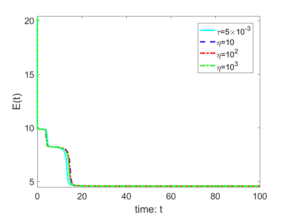
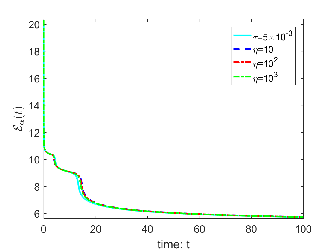
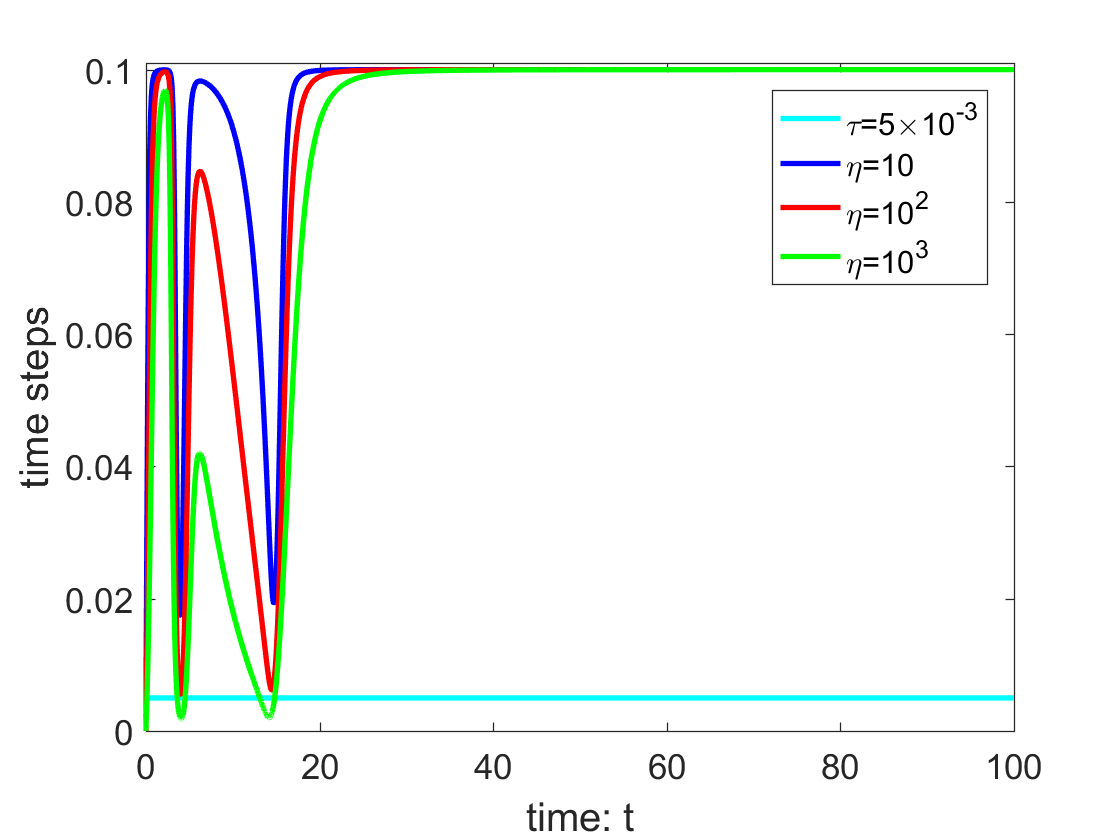
Figure 2: Numerical comparisons of energy evolutions using uniform time step and adaptive time-stepping strategy with different adaptive parameters $\eta$.

Table 4: Comparisons of CPU time (in seconds) and total time steps.

  Adaptive parameter $\eta=10$ $\eta=10^{2}$ $\eta=10^{3}$ uniform step CPU time 178.07 222.81 329.54 1666.83 Time steps 1156 1496 2669 20048  

The TFMBE model has obvious multi-scale behaviors in time [12] and the variable-step L1 scheme (2.7) is shown to be robustly stable and convergent on arbitrary time meshes, see Theorems 4.1 and 3.1. So certain adaptive time-stepping approach is reasonably adopted in our numerical simulations because it not only can capture the rapid changes of energy and numerical solution in a short time, but also can improve the calculation efficiency with large time-steps when the solution varies slowly.

We select the time steps according to the change rate of the numerical solution with the following adaptive time-stepping strategy, cf. [21],

$$\tau_{ada}=\max\bigg{\{}\tau_{\min},\frac{\tau_{\max}}{\sqrt{1+\eta\|\partial_{\tau}\phi^{n}\|^{2}}}\bigg{\}},$$

where $\tau_{\max}$ and $\tau_{\min}$ are the predetermined maximum and minimum size of time-steps, and $\eta$ is a user parameter to be determined. The space domain $(0,2\pi)^{2}$ is discretized by $128\times 128$ meshes during calculation. In additional, let $\tau_{N_{0}}:=\tau_{\min}$ when the graded mesh is applied in the initial cell $[0,T_{0}]$ and the adaptive time-stepping strategy is employed in the remainder interval $[T_{0},T]$, in which $N_{0}$ is determined by $\tau_{N_{0}}=t_{N_{0}}-t_{N_{0}-1}$.

In order to determine a suitable parameter $\eta$, we take $\tau_{\max}=10^{-1}$, $\tau_{\min}=10^{-3}$, and consider three different parameters $\eta=10,100$ and $10^{3}$. The reference solution is computed by using the uniform time step $\tau=5\times 10^{-3}$. As seen in Figure 2, the value of parameter $\eta$ evidently influences on the adaptive sizes of time steps. Specially, when $\eta=10^{3}$, the time-steps have the smallest fluctuation, and the L1 scheme can accurately capture the changes of original energy $E$ and modified energy $\mathcal{E}_{\alpha}$ over the time.

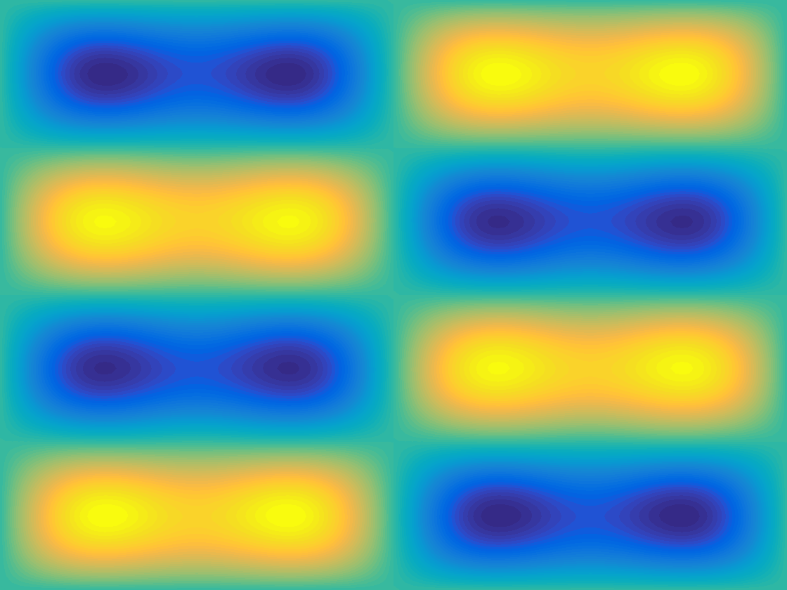
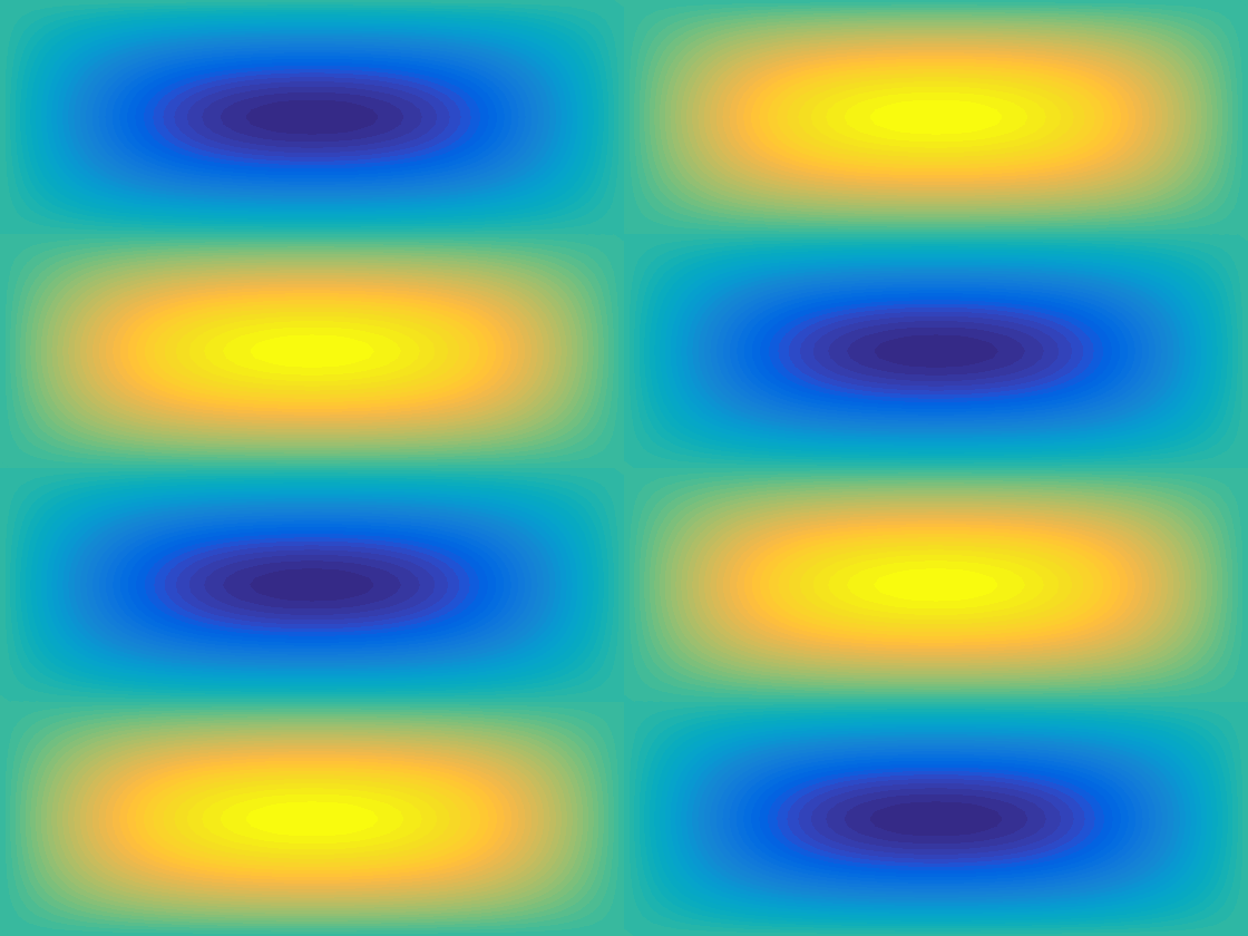
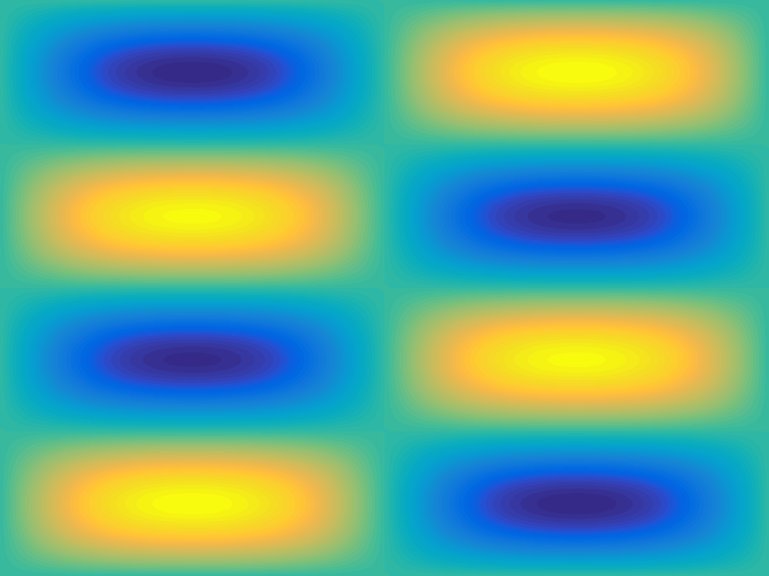
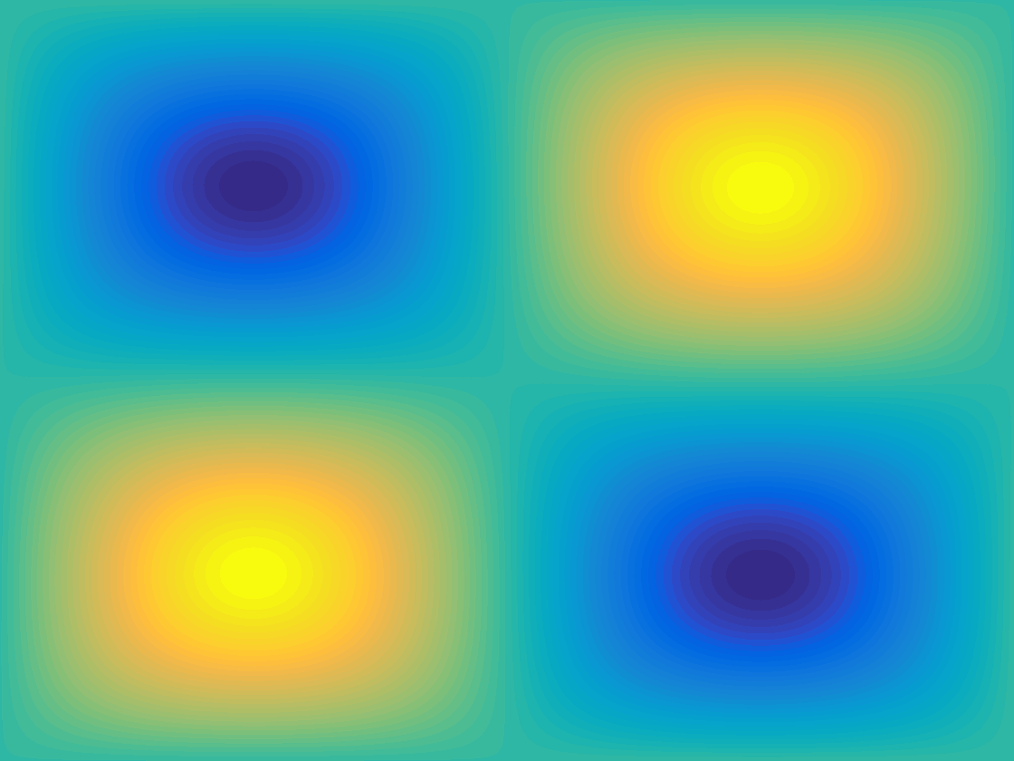
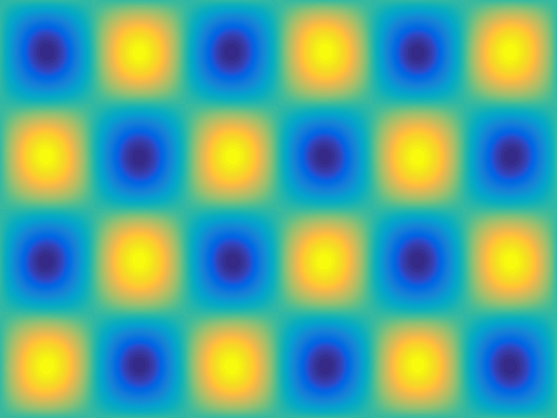
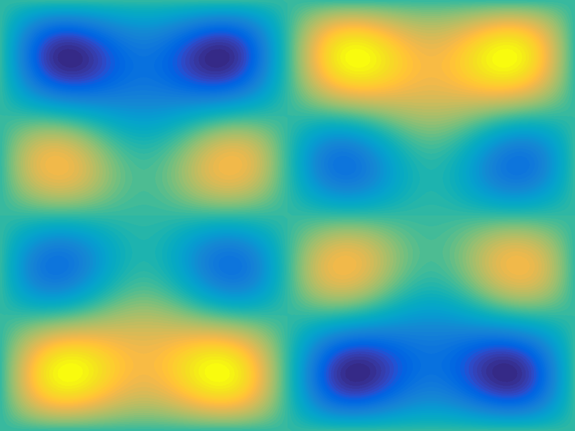
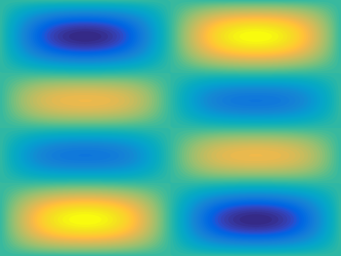
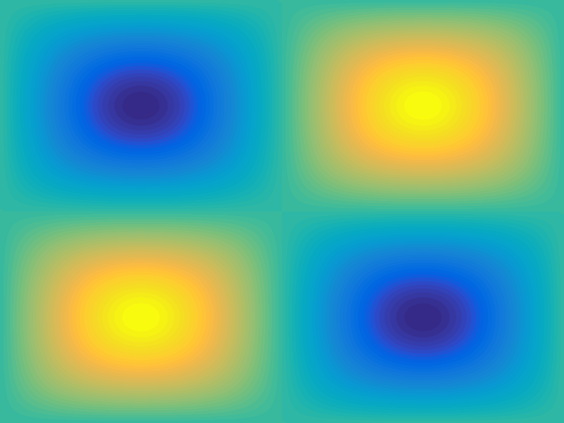
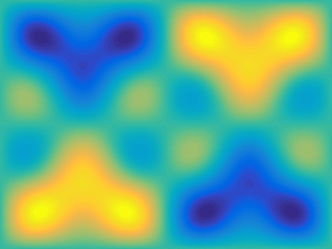
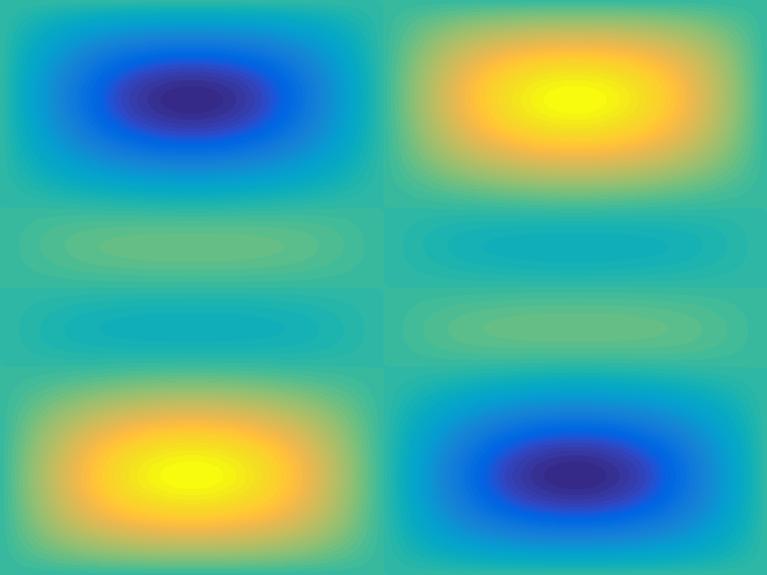
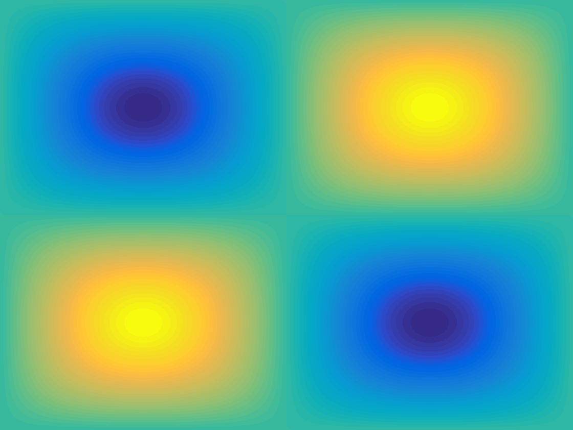
Figure 3: Time snapshots of TFMBE model (5.2) with $\varepsilon^{2}=0.1$ at $t=1.3,3.0,10,50$ (from left to right) for fractional orders $\alpha=0.4,0.7,0.9$ (from top to bottom), respectively.

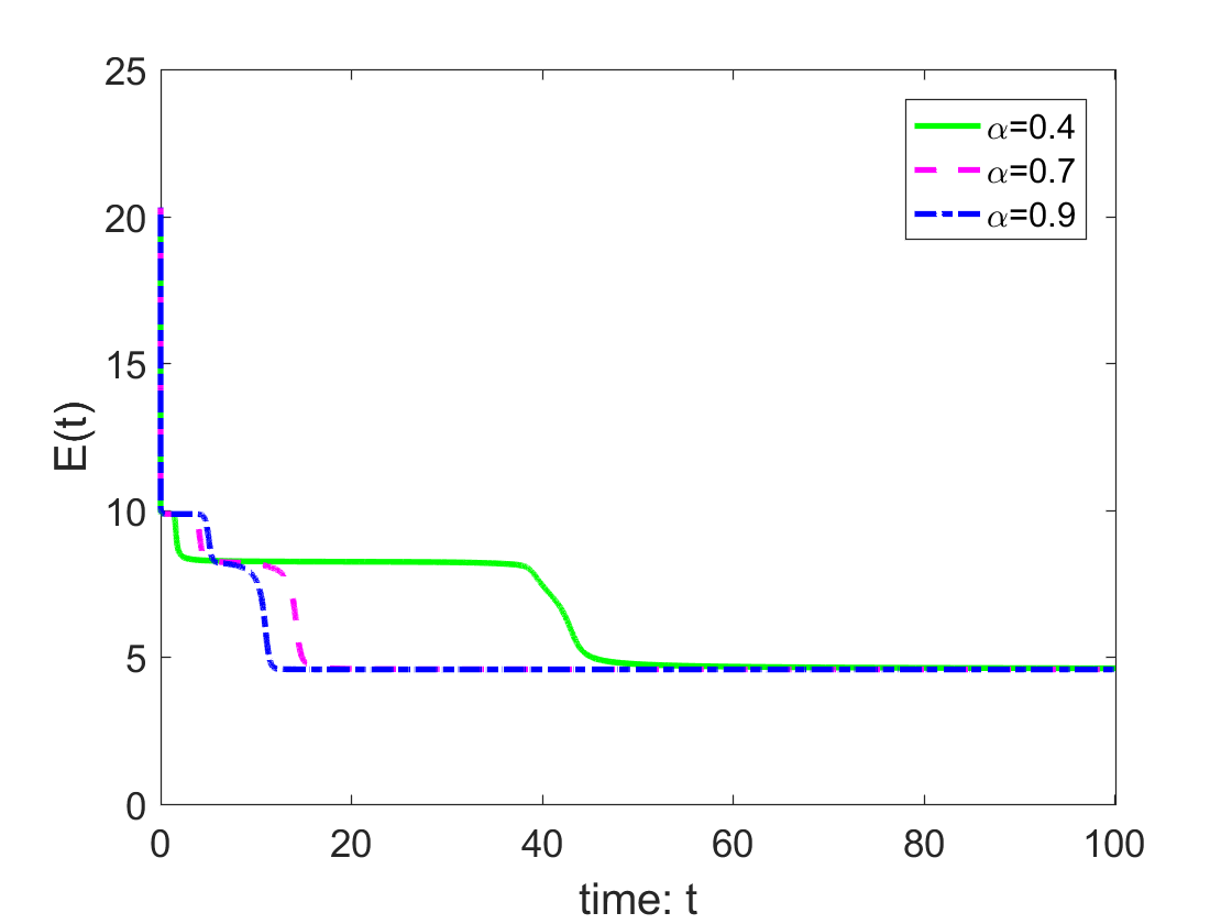
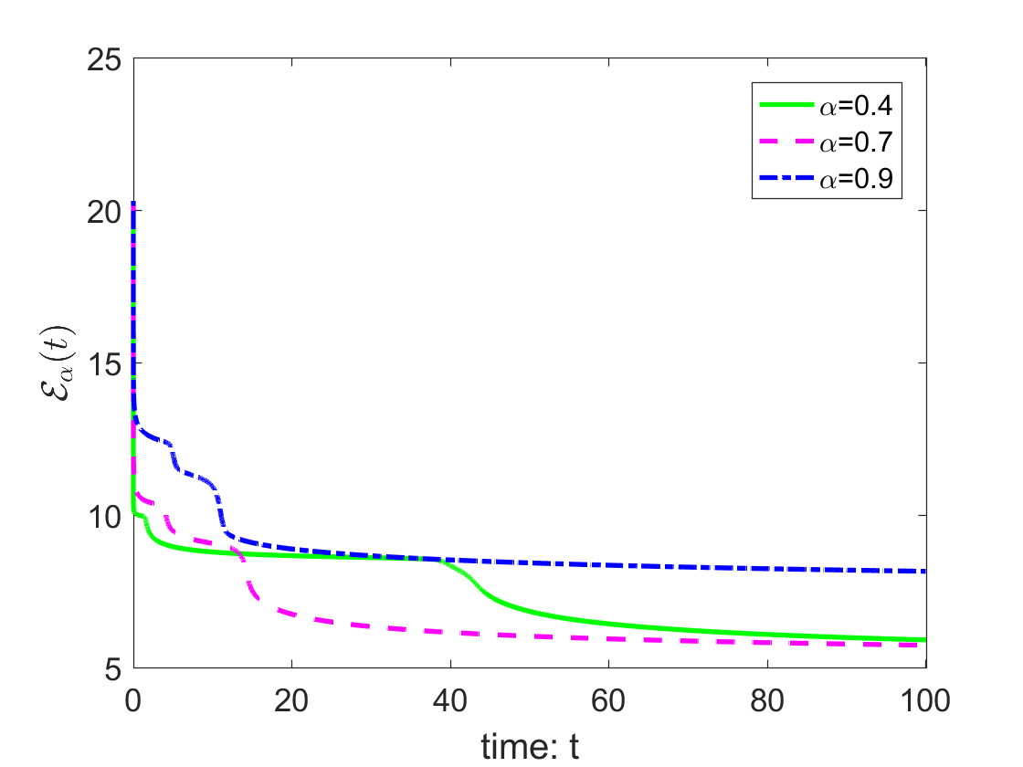
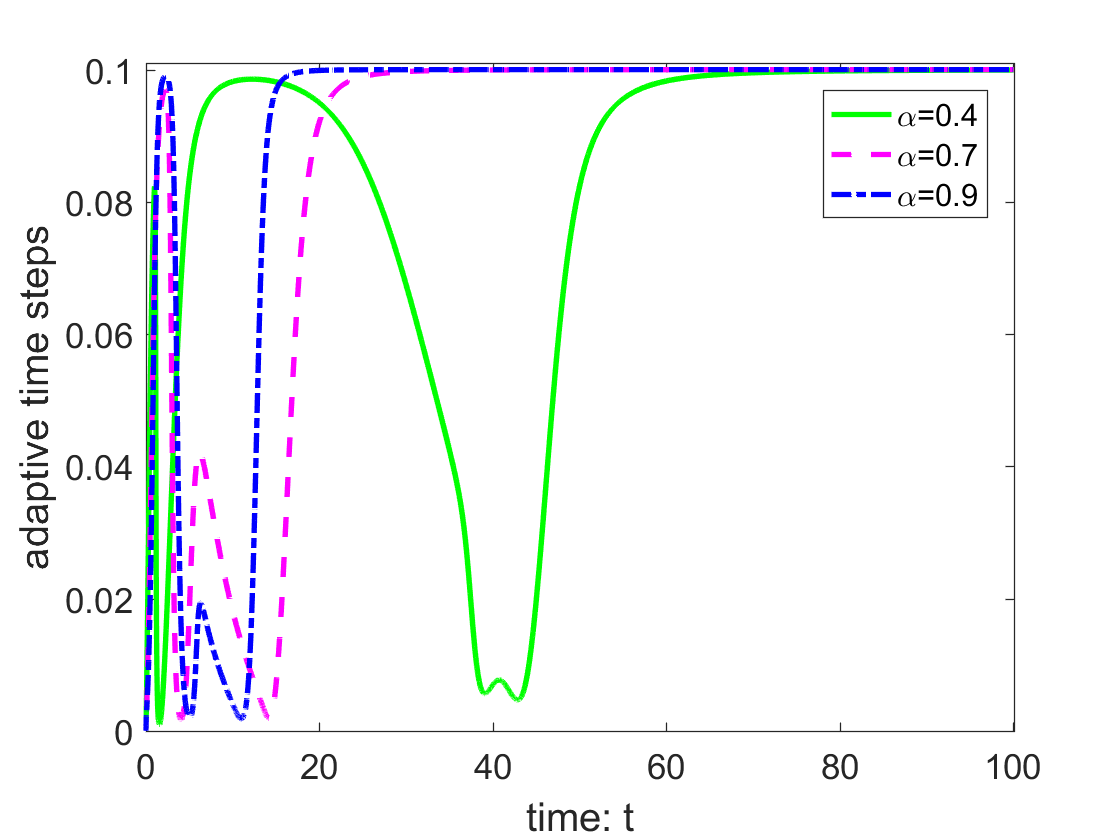
Figure 4: Curves of original energy $E(t)$, variational energy $\mathcal{E}_{\alpha}(t)$ and adaptive time steps $\tau_{n}$ generated for different fractional orders $\alpha$.

The corresponding CPU cost (in seconds) and the number of adaptive time levels are listed in Table 4. We observe that, at least for this example, $\eta=10^{3}$ is a good choice because it seems computationally more efficient than other cases using the parameters $\eta=10$, $\eta=10^{2}$, and using the uniform step size. As desired, the original energy $E$ monotonously decays over the time although we can not verify it theoretically. On the other hand, as expected by our analysis, the modified energy $\mathcal{E}_{\alpha}$ monotonously decays in the coarsening dynamics.

Next, by taking $\tau_{\max}=10^{-1}$, $\tau_{\min}=10^{-3}$ and the parameter $\eta=10^{3}$ in the above adaptive time-stepping strategy, we run the L1 scheme (2.7) for three different fractional orders $\alpha=0.4,0.7$ and $0.9$ until the final time $T=100$. The profiles of coarsening dynamics with different fractional orders $\alpha=0.4,0.7$ and 0.9 for the TFMBE model (1.5) are shown in Figure 3, where the snapshots of solution profiles are taken at time $t=1.3,3.0,10$ and 50, respectively. We observe that the coarsening rates are always dependent on the fractional order and the time period, but they all approach the steady state near $t=50$. The curves of original energy $E$ and the variational energy $\mathcal{E}_{\alpha}$ over the time interval $t\in[0,100]$ are depicted in Figure 4. The initial energy decays rapidly in all cases, while it decays slower for the smaller fractional order $\alpha$. As the time goes on, the evolution dynamics reach the same steady state in the end for different fractional orders. These results are in accordance with the previous observations in [5, 12].

6 Acknowledgements

The authors would like to thank Prof. Gong Yuezheng, Dr. Ji Bingquan and Ms. Zhu Xiaohan for their valuable suggestions.

References

- [1] A. Alikhanov. A priori estimates for solutions of boundary value problems for fractional-order equations. Diff. Equat., 46:660-666, 2010.
- [2] M. Ainsworth, and Z. Mao. Analysis and approximation of a fractional Cahn–Hilliard equation. SIAM J. Numer. Anal., 55: 1689-1718, 2017.
- [3] M. Al-Maskari, and S. Karaa. The time-fractional Cahn–Hilliard equation: analysis and approximation. IMA J. Numer. Anal., 2021, doi:10.1093/imanum/drab025.
- [4] W. Chen, S. Conde, C. Wang, X. Wang, and S. Wise. A linear energy stable scheme for a thin film model without slope selection. J. Sci. Comput., 52:546-562, 2012.
- [5] L. Chen, J. Zhao, W. Cao, H. Wang, and J. Zhang, An accurate and efficient algorithm for the time-fractional molecular beam epitaxy model with slope selection. Comput. Phys. Commun., 245:106842, 2019.
- [6] H. Chen, and M. Stynes. Blow-up of error estimates in time-fractional initial-boundary value problems. IMA J. Numer. Anal., 41: 974-997, 2021.
- [7] Q. Du, J. Yang, and Z. Zhou. Time-fractional Allen–Cahn equations: analysis and numerical methods. J. Sci. Comput., 85:42, 2020.
- [8] D. Eyre. Unconditionally gradient stable time marching the Cahn–Hilliard equation. Materials Research Society Symposium-Proceedings, 529:39, 1998.
- [9] W. Feng, C. Wang, S. Wise, and Z. Zhang. A second-order energy stable backward differentiation formula method for the epitaxial thin film equation with slope selection. Numer. Methods. Partial. Differential. Eq., 34:1975-2007, 2018.
- [10] Y. Gong, and J. Zhao. Energy-stable Runge-Kutta schemes for gradient flow models using the energy quadratization approach. Appl. Math. Lett., 94:224-231, 2019.
- [11] B. Ji, H.-L. Liao, and L. Zhang. Simple maximum priciple preserving time-stepping methods for time-fractional Allen-Cahn equation. Adv. Comput. Math., 46:37, 2020.
- [12] B. Ji, H.-L. Liao, Y. Gong, and L. Zhang. Adaptive second-order Crank-Nicolson time stepping schemes for time fractional molecular beam epitaxial growth models. SIAM J. Sci. Comput., 42:B738-B760, 2020.
- [13] B. Jin, B. Li and Z. Zhou, Numerical analysis of nonlinear subdiffusion equations. SIAM J. Numer. Anal., 56:1-23, 2018.
- [14] R. Kohn, and X. Yan. Upper bound on the coarsening rate for an epitaxial growth model. Commun. Pur. Appl. Math., 56:1549-1564, 2003.
- [15] H.-L. Liao, B. Ji and L. Zhang, An adaptive BDF2 implicit time-stepping method for the phase field crystal model. IMA J. Numer. Anal., 2020, doi:10.1093/imanum/draa075.
- [16] H.-L. Liao, W. Mclean, and J. Zhang. A discrete Grönwall inequality with application to numerical schemes for subdiffusion problems. SIAM J. Numer. Anal., 57:218-237, 2019.
- [17] H.-L. Liao, Y. Yan and J. Zhang. Unconditional convergence of a fast two-level linearized algorithm for semilinear subdiffusion equations. J. Sci. Comput., 80:1-25, 2019.
- [18] H.-L. Liao, T. Tang, and T. Zhou. Positive definiteness of real quadratic forms resulting from the variable-step approximation of convolution operators. 2020, submitted, arXiv:2011.13383v1.
- [19] H.-L. Liao and Z. Zhang. Analysis of adaptive BDF2 scheme for diffusion equations. Math. Comput., 90(329): 1207-1226, 2021.
- [20] H.-L. Liao, T. Tang, and T. Zhou. An energy stable and maximum bound preserving scheme with variable time steps for time fractional Allen–Cahn equation. SIAM J. Sci. Comput., 43(5): A3503-A3526, 2021.
- [21] H.-L. Liao, X. Zhu and J. Wang, The variable-step L1 time-stepping scheme preserving a compatible energy law for the time-fractional Allen–Cahn equation. Numer. Math. Theory Method Appl., 2021, accepted, arXiv:2102.07577v1.
- [22] W. McLean, K. Mustapha, R. Ali, and O. Knio. Regularity theory for time-fractional advection–diffusion–reaction equations. Comput. Math. Appl., 79(4):947–961, 2020.
- [23] D. Moldovan, and L. Golubovic. Interfacial coarsening dynamics in epitaxial growth with slope selection. Phys. Rev. E., 61:6190–6214, 2000.
- [24] J. Shen and X. Yang. Numerical approximations of Allen–Cahn and Cahn–Hilliard equations. Discrete. Contin. Dyn. Syst., 28:1669-1691, 2010.
- [25] J. Shen, and T. Tang. Spectral and High-Order Methods with Applications. Science Press, 2006.
- [26] J. Shen, J. Xu, and J. Yang. The scalar auxiliary variable (SAV) approach for gradient flows. J. Comput. Phys., 353:407-416, 2018.
- [27] J. Shen, J. Xu, and J. Yang. A new class of efficient and robust energy stable schemes for gradient flows. SIAM Rev., 61:474-506, 2019.
- [28] M. Stynes, E. O’riordan, and J. Gracia. Error analysis of a finite difference method on graded meshes for a time-fractional diffusion equation. J. Numer. Anal., 55(2):1057-1079, 2017.
- [29] T. Tang, H. Yu, and T. Zhou. On energy dissipation theory and numerical stability for time-fractional phase-field equations. SIAM J. Sci. Comput, 41(6):A3757-A3778, 2019.
- [30] C. Wang, X. Wang, and S. Wise. Unconditionally stable schemes for equations of thin film epitaxy. Discrete Contin. Dyn. Syst. Ser. A., 28:405-423, 2010.
- [31] S. Wise, C. Wang and J. Lowengrub. An energy-stable and convergent finite-difference scheme for the phase field crystal equation. SIAM J. Numer. Anal., 47(3):2269–2288, 2009.
- [32] C. Xu, and T. Tang. Stability analysis of large time-stepping methods for epitaxial growth models. SIAM J. Numer. Anal., 44:1759-1779, 2006.
- [33] J. Xu, Y. Li, S. Wu, and A. Bousquet. On the stability and accuracy of partially and fully implicit schemes for phase field modeling. Comput. Methods Appl. Mech. Engrg., 345:826-853, 2019.