Optimal Network Charge for Peer-to-Peer Energy Trading: A Grid Perspective

Abstract

Peer-to-peer (P2P) energy trading is a promising market scheme to accommodate the increasing distributed energy resources (DERs). However, how P2P to be integrated into the existing power systems remains to be investigated. In this paper, we apply network charge as a means for the grid operator to attribute transmission loss and ensure network constraints for empowering P2P transaction. The interaction between the grid operator and the prosumers is modeled as a Stackelberg game, which yields a bi-level optimization problem. We prove that the Stackelberg game admits an equilibrium network charge price. Besides, we propose a method to obtain the network charge price by converting the bi-level optimization into a single-level mixed-integer quadratic programming (MIQP), which can handle a reasonable scale of prosumers efficiently. Simulations on the IEEE bus systems show that the proposed optimal network charge is favorable as it can benefit both the grid operator and the prosumers for empowering the P2P market, and achieves near-optimal social welfare. Moreover, the results show that the presence of energy storage will make the prosumers more sensitive to the network charge price changes.

I Introduction

Driven by the technology advances and the pressure to advance low-carbon society, power systems are experiencing the steady increase of distributed energy resources (DERs), such as home batteries, electric vehicles (EVs), roof-top solar panels, and on-site wind turbines, etc. [1, 2, 3, 4]. As a result, the traditional centralized energy management is being challenged as the DERs on the customer side are beyond the control of the power grid operator. In this context, peer-to-peer (P2P) energy trading has emerged as a promising mechanism to account for the DERs [5]. P2P aims for a consumer-centric electricity market that allows the consumers with DERs (i.e., prosumer) to trade energy surplus or deficiency mutually [6, 7, 8]. The vision of P2P is to empower the prosumers to achieve the balance of supply and demand autonomously and economically by leveraging their complementary and flexible generation and consumption. P2P energy trading is beneficial to both the power grid operator and the prosumers. Specifically, P2P can bring monetary value to the prosumers by allowing them to sell surplus local renewable generation to their neighbors or vice verse [9, 13]. P2P also favors the power grid operation in term of reducing the cost of generation and transmission expansion to account for the yearly increasing demand as well as reducing transmission loss by driving local self-sufficiency [10].

Due to the widespread prospect, P2P energy trading mechanism has raised extensive interest from the research community. A large body of works has made efforts to address the matching of supply and demand bids for prosumers with customized preferences or interests. This is usually termed market clearing mechanisms. The mechanisms in discussion are diverse and plentiful, which can be broadly categorized by optimization-based approaches [11, 12, 13], auction schemes [10, 14], and bilateral contract negotiations [15, 16]. Quite a few of comprehensive and systematic reviews have documented those market clearing mechanisms, such as [17, 9, 18]. On top of that, a line of works has discussed the trust, secure, and transparent implementation of P2P market scheme by combing with the well-known blockchain technology, such as [19, 20].

The above studies are mainly focused on the business models of energy trading in virtual layer and in the shoes of prosumers. Whereas the energy exchanges in a P2P market require the delivery in physical layer taken by the power grid operator who is responsible for securing the transmission capacity constraints and compensating the transmission loss. In this regard, the effective interaction between the prosumers making energy transaction in virtual layer and the power grid operator delivering the trades in physical layer is essential for the successful deployment of P2P market scheme. The interaction requires to secure the economic benefit of prosumers in the P2P market as well as ensure the operation feasibility of power grid operator. This has been identified as one key issue that remains to be addressed [21].

Network charge which allows the grid operator to impose some grid-related cost on the prosumers for energy exchanges, has been advocated as a promising tool to bridge this interaction. Network charge is reasonable and natural considering many aspects. First of all, network charge is necessary for the power grid to attribute the network investment cost and the transmission loss [22]. In traditional power systems where customers trade energy with the power grid, such cost has been internalized in the electricity price, it is therefore natural to pass the similar cost with P2P to the prosumers via some price mechanisms. Besides, network charge can work as a means to shape the P2P energy trading market to ensure the feasible delivery of trades in physical layer taken by the grid operator [23]. Generally, network charge is charged by the trades, therefore it can be used to guide the behaviors of the prosumers in the P2P market. As a result, several recent works have relied on network charge to account for the grid-related cost or shape the P2P markets, such as [24, 22, 16]. Specifically, [24] has involved network charge in developing a decentralized P2P market clearing mechanism. The work [22] comparatively simulated three network charge models (i.e., unique model, electrical distance based model, and zonal model) on shaping the P2P market. The work [16] has relied on a network charge model to achieve ex-post transmission loss allocations across the prosumers. The above works have demonstrated that network charge can effectively shape the P2P transaction market. In addition, network charge can work as a tool to attribute grid-related cost and transmission loss which are actually taken by the grid operator. However, the existing works have mainly focused on studying how the network charge will affect the behaviors of prosumers in a P2P market instead of studying how the network charge price to be designed which couples the grid operator and the prosumers acting as independent stakeholders and playing different roles.

This paper fills the gap by jointly considering the power grid operator who provides transmission service and the prosumers who make energy transaction in a P2P market and propose an optimal network charge mechanism. Particularly, considering that the power grid operator and the prosumers are independent stakeholders and have different objectives, we model the interaction between the power grid operator and the prosumers as a Stackelberg game. First, the grid operator decides on the optimal network charge price to trade off the network charge revenue and the transmission loss considering the network constraints, and then the prosumers optimize their energy management (i.e., energy consuming, storing and trading) for maximum economic benefits. Our main contributions are:

• We propose a Stackelbeg game model to account for the interaction between the power grid operator imposing network charge price and the prosumers making energy transaction in a P2P market. The distributed renewable generators and energy storage (ES) devices on the prosumer side are considered. We prove that the Stackelberg game admits an equilibrium network charge price.

• To deal with the computational challenges of obtaining the network charge price, we convert the bi-level optimization problem yield by the Stackelberg game to a single-level mixed-integer quadratic programming (MIQP) by exploring the problem structures. The method can handle a reasonable scale of prosumers efficiently.

• By simulating the IEEE bus systems, we demonstrate that the network charge mechanism is favorable as it can benefit both the grid operator and the prosumers for empowering the P2P market. Moreover, it can provide near-optimal social welfare. In addition, we find that the presence of ES will make the prosumers more sensitive to the network charge price changes.

The rest of this paper is as: in Section II, we present the Stackelberg game formulation; in Section III, we propose a single-level conversion method; in Section VI, we examine the proposed network charge mechanism via case studies; in Section V, we conclude this paper and discuss the future work.

II Problem Formulation

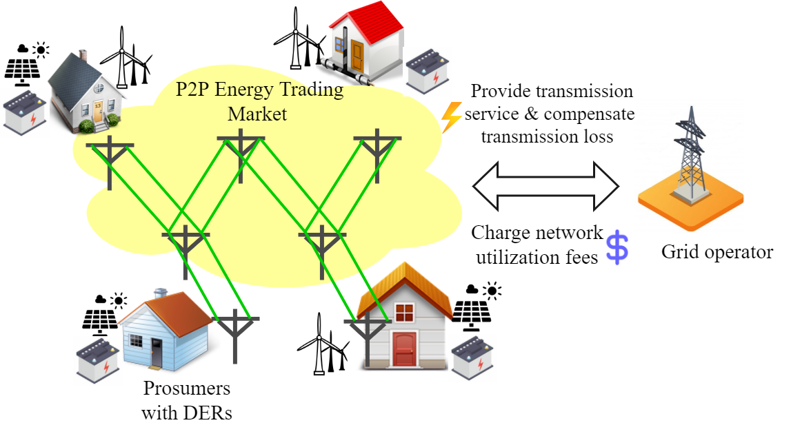
Figure 1: Interaction between the grid operator and a P2P energy trading market.

Fig. 1 shows the interaction between the grid operator and a P2P energy trading market to be discussed in this paper. By providing transmission service and compensating the transmission loss for empowering P2P trading, the grid operator plays the leading role by deciding the network charge price. In response, the prosumers with DERs (e.g., solar panels, wind turbines, ES, etc.) in the P2P market will optimize their optimal energy management (i.e., energy consuming, storing and trading) for maximum economic benefits. In this paper, we assume the grid operator and prosumers are independent stakeholder and are both profit-oriented, expecting to maximizing their own profit via the interaction. For the grid operator, the profit is evaluated by the network charge revenue minus the cost of transmission loss. For the prosumers, the profit is quantified by the utility (i.e., satisfaction) of consuming certain amount of energy and the energy cost such as the network charge payment. The objective of this paper is to determine the optimal network charge price that maximizes the grid profit while securing the prosumers’ profit in the P2P market.

II-A Network Charge Model

How to charge P2P energy trading for network utilization fee is still an open issue. One way in extensive discussion is based on the electrical distance and the volume of transaction. Specifically, if prosumer $i$ buys $p_{ij}$ [$\mathrm{kW}$] units of power from prosumer $j$ over an electrical distance of $d_{ij}$ [$\mathrm{km}$], the network charge is calculated as

$$\begin{split}&T(p_{ij})=\gamma d_{ij}p_{ij}\\ \end{split}$$ (1)

where $\gamma$[s$/($\mathrm{k}\mathrm{W}\cdot\mathrm{k}\mathrm{m}$)] is the network charge price determined by the grid operator, which represents the network utilization fee for per unit of energy transaction over per unit of electrical distance.

The electrical distance is determined by the electrical network topology and the measures used. For a given electrical network, there are several popular ways to measure the electrical distances as discussed in [25]. One of them is the Power Transfer Distance Factor (PTDF) which has been mostly used for network charge calculations (see [24, 22, 16] for examples). We therefore use the PTDF for measuring the electrical distances. For an electrical network characterized by transmission lines $\mathcal{L}$, the electrical distance between any trading peers $i,j$ based on PTDF is defined as

$$d_{ij}=\sum_{\ell\in\mathcal{L}}|{\rm PTDF}_{\ell,ij}|$$ (2)

where ${\rm PTDF}_{\ell,ij}$ represents the PTDF of prosumer $i,j$ related to transmission line $\ell\in\mathcal{L}$, which characterizes the estimated power flow change of line $\ell$ caused by per unit of energy transaction between prosumer $i$ and prosumer $j$ according to the DC power flow sensitivity analysis.

PTDF is directly derived from the DC power flow equations and the details can be found in [26]. In the following, we only summarize the main calculation procedures. For an electrical network characterized by $N$ buses and $L$ transmission lines, we first have the nodal acceptance matrix:

$$B_{ij}=\begin{cases}\sum_{k=1}^{N}\frac{1}{x_{ik}},&{\rm if}~{}j=i.\\ -\frac{1}{x_{ij}},&{\rm if}~{}j\neq i.\\ \end{cases}$$

where $x_{ij}$ represents the reactance of the line connecting bus $i$ and bus $j$.

We denote $\mathbf{B}_{r}$ as the sub-matrix of $\mathbf{B}$ which eliminates the row and column related to the reference bus $r$. Without any loss of generality, we specify bus $N$ as the reference bus, we therefore have $\mathbf{B}_{r}=\mathbf{B}[1:N-1,1:N-1]$ and the reverse $\mathbf{X}_{r}=\mathbf{B}_{r}^{-1}$. By setting zero row and column for the reference bus $r=N$, we have the augmented matrix:

$$\mathbf{X}=\begin{pmatrix}\mathbf{X}_{r}&\mathbf{0}\\ 0&0\end{pmatrix}$$

By using matrix $\mathbf{X}$, we can calculate the PTDF by

$${\rm PTDF}_{\ell,ij}=\frac{X_{mi}-X_{mj}-X_{ni}+X_{nj}}{x_{\ell}}$$ (3)

where $X_{mi},X_{mj},X_{ni},X_{nj}$ represent the elements of matrix $\mathbf{X}$ at row $m,n$ and column $i,j$, $\ell$ is the transmission line connecting bus $m$ and bus $n$.

An illustration example: we use the 5-bus system in Fig. 2 to illustrate the interpretation of electrical distances based on PTDF. Based on (2)-(3) and the reactance parameter $\mathbf{x}$, we can obtain the electrical distance $\mathbf{d}$ shown in Fig. 2 (b). Particularly, we have the electrical distance between bus $1$ and bus $3$: $d_{13}=0.2958+0.4930+0.2113+0.2958+0.2113=1.5072$ which are the PTDF of bus $1$ and bus $3$ related to the 5 transmission lines. As shown in Fig. 2 (a), the PTDF for bus $1,3$ can be interpreted as the total power flow changes of all transmission lines caused by per unit of energy transaction between the bus $1$ and $3$ according to the DC power flow analysis.

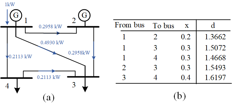
Figure 2: (a) Power flow changes of all transmission lines if bus $1$ transfers 1 $\mathrm{kW}$ power to bus $3$ based on DC power flow analysis. (b) The electrical distances between the buses based on PTDF for the 5-bus system.

II-B Stackelberg Game Formulation

As discussed, the interaction between the grid operator and the prosumers shows a hierarchical structure. This corresponds well to a Stackelberg game where the power grid behaves as the leader and the prosumers are followers. Before the formulation, we first define the main notations in TABLE I.

TABLE I: Main notations

Notation	Definition
$i,j$	Prosumer/bus index.
$t$	Time index.
$\gamma$	Network charge price.
$p_{ij,t}^{+}/p_{ij,t}^{-}$	Traded (buy or sell) energy between prosumer $i,j$.
$\theta_{i,t}$	Phase angle at bus $i$.
$\mathcal{P}_{i,t}$	Consumed or generated power of prosumer $i$.
$P_{i,t}$	Injected power at bus $i$.
$p_{i,t}^{\rm ch}/p_{it}^{\rm dis}$	Charged/discharged power of prosumer $i$’s ES.
$e_{i,t}$	Stored energy of prosumer $i$’s ES.
$U_{i,t}(\mathcal{P}_{i,t})$	Utility function of prosumer $i$.
$T(p_{ij,t}^{+})$	Network charge for trading $p_{ij,t}^{+}$ units of energy.
$F_{ij}^{\max}$	Transmission network capacity for line $(i,j)\in\mathcal{L}$.
$p_{i,t}^{\rm r}$	Renewable generation of prosumer $i$.
$C_{ij}^{\max}$	Max. trading power between prosumer $i,j$.
$e_{i}^{\min}/e_{i}^{\max}$	Min./max. stored energy of prosumer $i$’s ES.
$\mathcal{P}_{i,t}^{\min}/\mathcal{P}_{i,t}^{\max}$	Min./max. consumption/generation of prosumer $i$.

II-B1 Leader

In the upper level, the power grid optimizes the network charge price $\gamma$ to trade off the network charge revenue and the transmission loss considering the transmission network constraints. Network charge revenue is calculated by (1) and the power transmission loss is consolidated by the DC power flow of the transmission network [27]. We have the problem for the power grid:

$$\min_{\mathbf{x}_{U}}~{} {\rm Profit}=\sum_{t}\sum_{i}\sum_{j}\big{(}T(p_{ij,t}^{+})+T(p_{ij,t}^{-})\big{)}/2 {\rm P}_{U}$$ ()

$$\quad\quad~{}~{}-\rho\sum_{t}\sum_{(i,j)\in\mathcal{L}}b_{ij}(\theta_{i,t}-\theta_{j,t})^{2}$$

$${\rm s.t.} ~{}\gamma_{\min}\leq\gamma\leq\gamma_{\max}.$$ (4a)

$$\mathbf{B}\bm{\theta}_{t}=\mathbf{P}_{t},\forall t.$$ (4b)

$$\theta_{r,t}=0,\forall t.$$ (4c)

$$|(\theta_{i,t}-\theta_{j,t})b_{ij}|\leq F_{ij}^{\max},\forall(i,j)\in\mathcal{L},t.$$ (4d)

$$P_{i,t}={\textstyle\sum}_{j}p_{ij,t}^{-}-{\textstyle\sum}_{j}p_{ij}^{+},\forall i,t.$$ (4e)

$$\mathbf{P}^{\min}\leq\mathbf{P}_{t}\leq\mathbf{P}^{\max},\forall t.$$ (4f)

where the decision variables for the power grid operator are $\mathbf{x}_{\rm U}=[\gamma,\theta_{i,t}],\forall i,t$. We use $\mathbf{P}_{t}=[P_{i,t}],\forall i$ to denote the power injections at the buses and $b_{ij}$ denotes the admittance of the line connecting bus $i$ and bus $j$. We have $\gamma_{\min},\gamma_{\max}>0$ characterize the range of network charge price. We use the term $\rho{\textstyle\sum}_{(i,j)\in\mathcal{L}}b_{ij}(\theta_{i,t}-\theta_{j,t})^{2}=\rho{\textstyle\sum}_{(i,j)\in\mathcal{L}}P_{ij,t}^{2}/b_{ij}$ related to the power flows to quantify the consolidated transmission loss over the transmission networks $\mathcal{L}$ and $\rho$ is the transmission loss cost coefficient [27]. Constraints (4b) represent the DC power flow equations. Constraints (4c) specify the phase angle of reference bus $r$. Constraints (4d) model the transmission line capacity limits. In this paper, we use the DC power flow model to account for the transmission constraints and transmission loss. Whereas the proposed framework can be readily extended to AC power flow model by replacing (4b)-(4d) with the DistFlow [28] or the modified DistFlow [29] model. The nonconvex AC power flow model can be further convexified into a second-order cone program (SOCP) or a semi-definite program (SDP). Then the proposed method of this paper can still be used to solve the problem though with increased problem complexity.

II-B2 Followers

In the lower level, the prosumers in the P2P market will respond to the network charge price $\gamma$ for maximal economic benefit. We use $U_{i,t}(\mathcal{P}_{i,t})$ to represent the utility functions of prosumer $i$. Due to the presence of DERs, a prosumer could be a consumer or a producer. In this regard, $U_{i,t}(\mathcal{P}_{i,t})$ could represent the satisfaction of a customer for consuming $\mathcal{P}_{i,t}$ units of power or the cost of a producer for generating $\mathcal{P}_{i,t}$ units of energy. We also involve the distributed renewable generators and ES devices on the prosumer side in the formulation. In this paper, we assume the prosumers will cooperate with each other in the P2P market and formulate the problem as a centralized optimization problem as many existing works have proved that the cooperation can make all prosumer better off with some suitable ex-post profit allocation mechanisms (see [13, 30, 31] for examples). Since the network charge is measured by the traded power regardless of the direction, we distinguish the purchased power and sold power between prosumer $i$ and prosumer $j$ by $p_{ij,t}^{+}$ and $p_{ij,t}^{-}$. The problem to optimize the total prosumer profit considering network charge payment is presented below.

$$\max_{\mathbf{x}_{L}} ~{}~{}{\rm Profit}=\sum_{t}\sum_{i}U_{i,t}(\mathcal{P}_{i,t}) {\rm P}_{L}$$ ()

$$\quad\quad\quad-\sum_{t}\sum_{i}\sum_{j}\big{(}T(p^{+}_{ij,t})+T(p^{-}_{ij,t})\big{)}/2$$

s.t. $$p_{ij,t}^{+}=p^{-}_{ji,t},~{}~{}~{}\forall i,j,t.$$ (5a)

$$0\leq p_{ij,t}^{+}\leq C_{ij}^{\max},~{}~{}\forall i,j,t.$$ (5b)

$$0\leq p_{ij,t}^{-}\leq C_{ij}^{\max},~{}~{}\forall i,j,t.$$ (5c)

$$\mathcal{P}_{i,t}\leq p_{i,t}^{\rm r}\!+\!p_{i,t}^{\rm dis}\!-\!p_{i,t}^{\rm ch}\!+\!{\textstyle\sum}_{j}p_{ij,t}^{+}\!-\!{\textstyle\sum}_{j}p_{ij,t}^{-},\forall i,t.$$ (5d)

$$\mathcal{P}_{i,t}^{\min}\leq\mathcal{P}_{i,t}\leq\mathcal{P}_{i,t}^{\max},~{}\forall i,t.$$ (5e)

$$e_{i,t+1}=e_{i,t}+p_{i,t}^{\rm ch}\eta-p_{i,t}^{\rm dis}/\eta,~{}\forall i,t.$$ (5f)

$$0\leq p_{i,t}^{\rm ch}\leq P_{i}^{\rm ch,\max},~{}~{}\forall i,t.$$ (5g)

$$0\leq p_{i,t}^{\rm dis}\leq P_{i}^{\rm dis,\max},~{}~{}\forall i,t.$$ (5h)

$$e_{i}^{\min}\leq e_{i,t}\leq e_{i}^{\max},\forall i,t.$$ (5i)

where the decision variables for the prosumers are $\mathbf{x}_{L}=[p_{ij,t}^{+},p_{ij,t}^{-},\mathcal{P}_{i,t},p_{i,t}^{\rm ch},p_{i,t}^{\rm dis},e_{i,t}],\forall i,t$. Constraints (5a) model the consistence of energy transaction between the sellers and the buyers. Since the transmission loss is compensated by the power grid operator, we have the amount of energy that prosumer $i$ buys from prosumer $i$ equals that prosumer $j$ sells to prosumer $i$. Constraints (5b)-(5c) impose the transaction limits between the trading peers. Constraints (5d) ensure the load balance of each prosumer. Particularly, we use inequality to capture the case where some renewable generation is curtailed. Constraints (5e) characterize the demand or supply flexibility of the prosumers. Constraints (5f) tracks the stored energy of prosumers’ ES with $\eta\in(0,1)$ denoting the charging/discharging efficiency. Constraints (5g)-(5h) impose the charging, discharging and stored energy capacity limits. In this paper, we focus on the energy trading among the prosumers in the P2P market. For the case where the prosumers also trade electricity with the power grid, the proposed model can be readily extended by adding the cost or revenue related to the energy trading with the grid to the prosumers’ objective in the lower-level problem (${\rm P}_{L}$).

II-B3 Piece-wise linear utility function

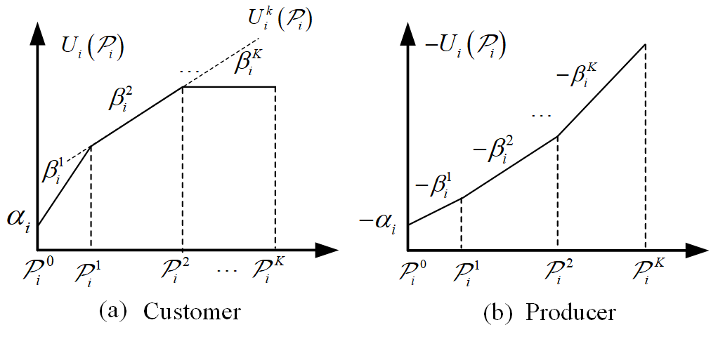
Figure 3: (a) Piece-wise linear (PWL) utility function for a consumer $\nabla U_{i}(\mathcal{P}_{i})\geq 0$. (b) Piece-wise linear utility (PWL) function for a producer $\nabla U_{i}(\mathcal{P}_{i})\leq 0$ (time $i$ is omitted).

This paper employs concave piece-wise linear (PWL) utility functions to capture the prosumers’ demand or supply flexibility as shown in Fig. 3. The motivation behind is that PWL functions are universal and can approximate all types of utility functions, such as quadratic and logarithmic [32]. We may obtain the PWL utility functions by linearizing non-linear utility functions or directly learn it from data [33]. Due to the presence of DERs, the prosumer could be a consumer in energy deficiency or a producer with energy surplus. This could be universally formulated by the PWL utility function but with the opposite sign of the slopes. We use Fig. 3 (a) and (b) to show the two scenarios (time $i$ is omitted): if the slope of the PWL utility function is non-negative $U_{i}(\mathcal{P}_{i})\geq 0$, the prosumer plays the role of customer and the prosumer will play the role of producer if $U_{i}(\mathcal{P}_{i})\leq 0$. As shown in Fig 3, a general PWL utility function composed of $K$ segments is characterized by the transition points and slopes: $\mathcal{P}^{k}_{i}$ and $\beta^{k}_{i},k=1,2,\cdots,K$. The function associated with the $k$-th segment can be described as

$$U^{k}_{i}(\mathcal{P}_{i})\!= \alpha_{i}\!+\!\sum_{\ell=1}^{k-1}\beta^{\ell}_{i}\left(\mathcal{P}^{\ell}_{i}\!-\!\mathcal{P}^{\ell-1}_{i}\right)\!\!+\!\!\beta^{k}_{i}\left(\mathcal{P}_{i}\!-\!\mathcal{P}^{k-1}_{i}\right),\forall i,k.$$ (6)

where $\alpha_{i}$ is the constant component of prosumer $i$’s utility function, which could represent the satisfaction level of a prosumer for consuming zero unit of energy or the start-up generation cost for a producer. It is easy to note that we have $U_{i}(\mathcal{P}_{i})=U_{i}^{k}(\mathcal{P}_{i})$ if $\mathcal{P}_{i}\in[\mathcal{P}^{k-1}_{i},\mathcal{P}^{k}_{i})$.

For the proposed Stackelberg game, we have the following results regarding the existence of equilibrium.

Theorem 1.

The Stackelberg game (${\rm P}_{U}$)-(${\rm P}_{L}$) admits an equilibrium.

Proof.

For the lower-level problem (${\rm P}_{L}$), we note that the problem is compact and convex with any given network charge price $\gamma$. This implies that the optimal solution for the lower-level problem (${\rm P}_{L}$) always exists and can be expressed by $\mathbf{x}_{L}(\gamma)$. By substituting the closed-form solution $\mathbf{x}_{L}(\gamma)$ (if explicitly available) into the upper-level problem (${\rm P}_{U}$) and by expressing the phase angle decision variables $\bm{\theta}$ with the power flows determined by the lower-level problem solution $\mathbf{x}_{L}(\gamma)$, we can conclude a single-level optimization problem for the Stackelberg game with the only bounded decision variables $\gamma\in[\gamma^{\min},\gamma^{\max}]$, which will yield at least one optimal solution. This implies that the proposed Stackelberg game adopts at least one Stackelberg equilibrium. ∎

Remark 1.

The existence of the Stackelberg equilibrium implies that the proposed optimal network charge model can yield an optimal network charge price that maximizes the profit of the grid operator while considering the cost-aware behaviors of the prosumers in the P2P market.

III Methodology

Note that the optimal network charge associates with the equilibrium of the Stackelberg game (${\rm P}_{U}$)-(${\rm P}_{L}$) which yields a bi-level optimization. Bi-level optimization is generally NP-hard and computationally intensive [34]. This section proposes a method to convert the bi-level problem to a single-level problem that can accommodate a reasonable scale of prosumers by exploring the problems structures. To achieve this goal, we first restate the lower-level problem (${\rm P}_{L}$) as

$$\max_{\mathbf{x}_{L}} ~{}{\rm Profit}=\sum_{t}\sum_{i}u_{i,t}-\sum_{t}\sum_{i}\sum_{j}T(p_{ij,t}^{+}) {\rm P}^{{}^{\prime}}_{L}$$ ()

$${\rm s.t.}~{} 0\leq p_{ij,t}^{+}\leq C_{ij}^{\max}:~{}\quad\quad~{}~{}\underline{\nu}_{ij,t},\overline{\nu}_{ij,t}\geq 0,~{}\forall i,j,t.$$ (7a)

$$\mathcal{P}_{i,t}\!\leq\!p_{i,t}^{\rm r}\!+\!p_{i,t}^{\rm dis}\!-\!p_{i,t}^{\rm ch}\!+\!{\textstyle\sum}_{j}p_{ij,t}^{+}\!-\!\!{\textstyle\sum}_{j}p_{ji,t}^{+}:$$

$$\quad\quad\quad\quad\quad\quad\quad\quad\quad\quad\quad\quad\quad\quad~{}~{}\mu_{i,t}\geq 0,\forall i,t.$$ (7b)

$$\mathcal{P}_{i}^{\min}\leq\mathcal{P}_{i,t}\leq\mathcal{P}^{\max}_{i}:~{}\quad\quad~{}~{}\underline{\sigma}_{i,t},\overline{\sigma}_{i,t}\geq 0,~{}\forall i,t.$$ (7c)

$$e_{i,t+1}=e_{i,t}+p_{i,t}^{\rm ch}\eta-p_{i,t}^{\rm dis}/\eta:\quad~{}\mu_{i,t}^{\rm e}\in\mathbb{R},~{}\forall i,t.$$ (7d)

$$0\leq p_{i,t}^{\rm ch}\leq P_{i}^{\rm ch,\max}:\quad\quad\quad~{}~{}\underline{\mu}^{\rm ch}_{i,t},\overline{\mu}_{i,t}^{\rm ch}\geq 0,~{}\forall i,t.$$ (7e)

$$0\leq p_{i,t}^{\rm dis}\leq P_{i}^{\rm dis,\max}:\quad\quad~{}~{}~{}\underline{\mu}_{i,t}^{\rm dis},\overline{\mu}_{i,t}^{\rm dis}\geq 0,~{}\forall i,t.$$ (7f)

$$e_{i}^{\min}\!\leq\!e_{i,t}\leq e_{i}^{\max}:\quad\quad\quad~{}~{}~{}\underline{\mu}_{i,t}^{\rm e},\overline{\mu}_{i,t}^{\rm e}\geq 0,~{}\forall i,t.$$ (7g)

$$u_{i,t}\leq U_{i}^{k}(\mathcal{P}_{i,t}):\quad\quad\quad\quad\quad\quad\delta_{i,k,t}\geq 0,~{}\forall i,k,t.$$ (7h)

where the decision variable $\mathbf{P}^{-}=[p_{ij,t}^{-}],\forall i,j,t$ are removed based on $p_{ij,t}^{+}=p_{ji,t}^{-},\forall i,j,t$. Besides, some auxiliary variables $u_{i,t}$ are introduced to relax the non-smooth prosumer utility functions. Since the utility function is concave, it is easy to prove that (${\rm P}^{{}^{\prime}}_{L}$) is equivalent to (${\rm P}_{L}$). Additionally, the dual variables for the constraints are defined the right-hand side.

For the reformulated lower-level problem (${\rm P}^{{}^{\prime}}_{L}$), we can draw the Karush–Kuhn–Tucker (KKT) conditions [35]. We first have the first-order optimality conditions:

$$\partial L/\partial\mathcal{P}_{i,t}\!=\!\mu_{i,t}\!-\!\underline{\sigma}_{i,t}\!+\!\overline{\sigma}_{i,t}\!-\!{\textstyle\sum}_{k}\delta_{i,k,t}\nabla U_{i,t}^{k}(\mathcal{P}_{i,t})\!=\!0$$ (8a)

$$\partial\mathbb{L}/\partial p_{ij,t}^{+}\!=\!\gamma d_{ij}-\underline{\nu}_{ij,t}+\overline{\nu}_{ij,t}-\mu_{i,t}+\mu_{j,t}=0$$ (8b)

$$\partial\mathbb{L}/\partial u_{i,t}\!=\!-1+{\textstyle\sum}_{k}\delta_{i,k,t}=0$$ (8c)

$$\partial\mathbb{L}/\partial p_{i,t}^{\rm ch}\!=\!\mu_{i,t}-\mu_{i,t}^{\rm e}\eta-\underline{\mu}_{i,t}^{\rm ch}=0$$ (8d)

$$\partial\mathbb{L}/\partial p_{i,t}^{\rm dis}\!=\!-\mu_{i,t}+\mu_{i,t}^{\rm e}/\eta-\underline{\mu}_{i,t}^{\rm dis}+\overline{\mu}_{i,t}^{\rm dis}=0$$ (8e)

$$\partial L/\partial e_{i,t}\!=\!-\mu_{i,t}^{\rm e}\!+\!\mu_{i,t-1}^{\rm e}\!-\!\underline{\mu}_{i,t-1}^{\rm e}\!+\!\overline{\mu}_{i,t-1}^{\rm e}=0,\forall t>1$$ (8f)

where we use $\mathbb{L}$ to denote the Lagrangian function associated with (${\rm P}^{{}^{\prime}}_{L}$). Based on (6), we have $\nabla U_{i,t}^{k}(\mathcal{P}_{i,t})=\beta_{i}^{k}$ which represents the slope of the prosumer $i$’s utility function at the $k$-th segment.

In addition, we have the complementary constraints for the inequality constraints (7a)-(7h). Using (7d) as an example, we have the complementary constraints:

$$\mu_{i,t}\big{(}\mathcal{P}_{i,t}\!-\!p_{i,t}^{\rm r}\!-\!p_{i,t}^{\rm dis}\!+\!p_{i,t}^{\rm ch}\!-\!{\textstyle\sum}_{j}p_{ij,t}^{+}\!+\!\!{\textstyle\sum}_{j}p_{ji,t}^{+}\big{)}\!=\!0,\forall i,t.$$ (9)

The general way to handle the non-linear complementary constraints is to introduce binary variables to relax the constraints (see [36] for an example). This could be problematic for problem (${\rm P}^{{}^{\prime}}_{L}$) due to the large number of inequality constraints. To deal with the computational challenges, we make use of the linear programming (LP) structure of problem (${\rm P}^{{}^{\prime}}_{L}$). For a LP, we have the strong duality and the complementary constraints are interchangeable (see [37], Ch4, pp. 147 for detailed proof). Therefore, we use the strong duality condition for problem (${\rm P}^{{}^{\prime}}_{L}$) to replace the complementary constraints, such as (9). We have the strong duality for problem (${\rm P}^{{}^{\prime}}_{L}$):

$$\begin{split}&\!-\!\sum_{t}\sum_{i}\sum_{j}\overline{\nu}_{ij,t}C_{ij}^{\max}\!-\!\sum_{t}\sum_{i}\mu_{i,t}p_{i,t}^{\rm r}\!\!+\!\!\sum_{t}\sum_{i}\underline{\sigma}_{i,t}\mathcal{P}_{i,t}^{\min}\\ &\!-\!\!\sum_{t}\!\sum_{i}\overline{\sigma}_{i,t}\mathcal{P}_{i,t}^{\max}\!\!-\!\!\sum_{t}\!\!\sum_{i}\overline{\mu}_{i,t}^{\rm ch}P_{i}^{\rm ch,\max}\!\!-\!\!\sum_{t}\!\sum_{i}\overline{\mu}_{i,t}^{\rm dis}P_{i}^{\rm dis,\max}\\ &\!\!+\!\!\sum_{t}\sum_{i}\underline{\mu}_{i,t}^{\rm e}e_{i}^{\min}\!\!-\!\!\sum_{t}\sum_{i}\overline{\mu}_{i,t}^{\rm e}e_{i}^{\max}\!\!-\!\!\sum_{t}\sum_{i}\sum_{k}\delta_{i,k,t}U_{i}^{k}(0)\\ &=\sum_{t}\sum_{i}\sum_{j}T(p_{ij,t}^{+})-\sum_{t}\sum_{i}u_{i,t}\end{split}$$ (10)

Note that the strong duality (10) can be used to eliminate the large number of non-linear complementary constraints but requires to tackle the bi-linear terms related to the network charge calculations: $T(p_{ij,t}^{+})=\gamma d_{ij}p_{ij,t}^{+}$. To handle such bi-linear terms, we discretize the network charge price and convert the non-linear terms into mixed-integer constraints. Specifically, we first define an auxiliary variable $Z$:

$$Z=\sum_{t}\sum_{i}\sum_{j}d_{ij}p_{ij,t}^{+}$$

We thus have the total network charge for P2P transaction:

$$\begin{split}\sum_{t}\sum_{i}\sum_{j}T(p_{ij,t}^{+})=\gamma Z\end{split}$$ (11)

We discretize the range of network charge price $[\gamma_{\min},\gamma_{\max}]$ into $L$ levels $\{\gamma_{1},\gamma_{2},\cdots,\gamma_{L}\}$ with an equal interval $\Delta\gamma=(\gamma_{\max}-\gamma_{\min})/L$. Accordingly, we introduce the binary variables $\mathbf{x}=[x_{\ell}],\ell=1,2,\cdots,L$ to indicate which level of network charge price is selected, we thus have

$$\gamma Z={\textstyle\sum}_{\ell=1}^{L}x_{\ell}\gamma_{\ell}Z$$ (12)

$${\textstyle\sum}_{\ell=1}^{L}x_{\ell}=1,~{}x_{\ell}\in\{0,1\}$$ (13)

Note that the network charge calculations rely on the product of binary variable $x_{\ell}$ and continuous variable $Z$. This can be equivalently expressed by the integer algebra:

$$\quad\quad~{}-Mx_{\ell}\leq Y_{\ell}\leq Mx_{\ell}$$ (14)

$$-M(1-x_{\ell})\leq Z-Y_{\ell}\leq M(1-x_{\ell})$$ (15)

where we have $\gamma Z=\sum_{\ell=1}^{L}\gamma_{\ell}Y_{\ell}$ and $M$ is a sufficiently large positive constant.

By plugging ${\textstyle\sum}_{t}{\textstyle\sum}_{i}{\textstyle\sum}_{j}T(p_{ij,t}^{+})=\gamma Z={\textstyle\sum}_{\ell=1}^{L}\gamma_{\ell}Y_{\ell}$ in (10), and by replacing the lower level problem (${\rm P}^{{}^{\prime}}_{L}$) with KKT conditions, we have the following single-level mixed-integer quadratic programming (MIQP):

$$\max_{\mathbf{x}_{U},\mathbf{x}_{L},\bm{\lambda}}~{} \text{Profit}=\sum_{\ell=1}^{L}\gamma_{\ell}Y_{\ell}-\rho\!\!\!\sum_{(i,j)\in\mathcal{L}}\!\!\!b_{ij}(\theta_{i}-\theta_{j})^{2} P$$ ()

$$\text{s.t.}~{}\eqref{eq:10a}-\eqref{eq:10h}.~{}~{}~{}~{}~{}~{}~{}~{}\text{Primal constraints}$$

$$~{}~{}~{}~{}\eqref{eq:11a}-\eqref{eq:11f}.~{}~{}~{}~{}~{}~{}~{}~{}~{}\text{KKT conditions}$$

$$~{}~{}~{}~{}\eqref{eq:strong_duality},\eqref{eq:linearization}-\eqref{eq:integer_algebra2}~{}~{}~{}~{}\text{Strong~{}duality}$$

where $\lambda=[\bm{\underline{\nu}},\bm{\overline{\nu}},\bm{\mu},\bm{\underline{\sigma}},\bm{\overline{\sigma}},\bm{\mu}^{\rm e},\bm{\underline{\mu}}^{\rm ch},\bm{\overline{\mu}}^{\rm ch},\bm{\underline{\mu}}^{\rm dis},\bm{\overline{\mu}}^{\rm dis},\bm{\underline{\mu}}^{\rm e},\bm{\overline{\mu}}^{\rm e},\bm{\delta}]$ are the dual variables. Note that this single-level conversion favors computation as the number of binary variables ($L$) is only determined by the granularity of network charge discretization and independent of the scale of prosumers, making it possible to accommodate a reasonable scale of prosumers.

IV Case Studies

In this section, we evaluate the performance of the proposed network charge mechanism via simulations. We first use IEEE 9-bus system to evaluate the effectiveness of the solution method, the existence of equilibrium network charge price, and the social welfare. We further evaluate the performance on the larger electrical networks including IEEE 39-bus, 57-bus, and 118-bus systems. Particularly, we compare the results with and without ES on the prosumer side in the case studies.

TABLE II: Simulation set-ups

Param.	Definition	Value
$T$	Time periods	24
$\alpha_{i,t}$	Proumer PWL utility constant	0
$\beta_{i,t}^{k}$	Prosumer PWL utility slopes	$[0,1]$
$K$	Prosumer PWL utility segments	2 or 3
$[\gamma^{\min},\gamma^{\max}]$	Network charge price range	[0, 1] $\mathrm{s}\$\mathrm{/}\mathrm{(}\mathrm{k}\mathrm{W}\cdot\mathrm{k}\mathrm{m}\mathrm{)}$
$\Delta\gamma$	Network charge price discretization	0.02 $\mathrm{s}\$\mathrm{/}\mathrm{(}\mathrm{k}\mathrm{W}\cdot\mathrm{k}\mathrm{m}\mathrm{)}$
$L$	Network charge discretization levels	51
$e_{i}^{\min}/e_{i}^{\max}$	Min./max storaged energy of ES	0/60 $\mathrm{kW}\text{\,}\mathrm{h}$
$P_{i}^{\rm ch,\max}$	Max. charging power	50 $\mathrm{kW}$
$P_{i}^{\rm dis,\max}$	Max. discharging power	50 $\mathrm{kW}$
$\eta$	Charging/discharging efficiency	0.9
$\rho$	Transmission loss cost coefficient	0.01

IV-A Simulation Set-ups

We set up the case studies by rescaling the real building load profiles [38] and the renewable generation profiles (i.e., wind and solar) [39]. To capture the demand flexibility, we set the lower prosumer demand as $\mathcal{P}_{i,t}^{\min}=0$ (we focus on the flexible demand) and the upper prosumer demand as $\mathcal{P}_{i,t}^{\max}=\text{\emph{demand profile}}_{i,t}+30$ $\mathrm{kW}$. For each time period $t$, we uniformly generate the slopes of prsumer PWL utility functions in $\beta_{i,t}^{k}\in[0,1]$ with $K=2$ or $3$ segments (we only consider customers in the following studies and the producers can be included by setting $\beta_{i,t}^{k}\in[-1,0]$ if exist). We set the constant components of PWL utility function as $\alpha_{i,t}=0$ for all customers. Correspondingly, we equally divide the ranges of prosumer demand $[\mathcal{P}^{\min}_{i,t},\mathcal{P}^{\max}_{i,t}]$ into $K=2$ or $3$ segments to obtain the PWL utility function transition points $\mathcal{P}^{k}_{i,t}$. We simulate the P2P market for 24 periods with a decision interval of one hour. The settings for the above parameters and the prosumers’ ES are gathered in TABLE II. Particularly, we set the range of network charge price as $\gamma^{\min}=0$ and $\gamma^{\max}=1.0$ $\mathrm{s}\$\mathrm{/}\mathrm{(}\mathrm{k}\mathrm{W}\cdot\mathrm{k}\mathrm{m}\mathrm{)}$ and the discretization interval as $\Delta\gamma=0.02$ $\mathrm{s}\$\mathrm{/}\mathrm{(}\mathrm{k}\mathrm{W}\cdot\mathrm{k}\mathrm{m}\mathrm{)}$ based on the simulation results of Section IV-B, which suggest such settings are expected to provide solutions with sufficiently high accuracy. Besides, the electrical distances measured by PTDF for the concerned bus systems are directly obtained with the method in Section II-A.

In this paper, we refer to the P2P market with the proposed network charge as Optimal P2P. The network charge price is obtained by solving problem ($P$) with the off-the-shelf solvers. In the following studies, we compare Optimal P2P with No P2P (P2P transaction is forbidden), Free P2P (P2P transaction is allowed without any network charge form the prosumers) and Social P2P (P2P transaction is determined by maximizing the social profit which is the sum of grid operator profit and prosumer profit defined in (${\rm P}_{U}$) and (${\rm P}_{L}$)). Note that the network charge with Social P2P will be internalized as the grid operator and the prosumers are unified as a whole. For Free P2P, the grid operator has no manipulation on the P2P market and the optimal transaction can be determined by directly solving the lower-level problem (${\rm P}_{L}$) by removing the network charge components (To ensure the uniqueness of the solution, we keep the network charge but set a sufficiently small value). In addition, we examine the different markets without and with ES on the prosumer side. For the case without ES, we set $e_{i}^{\max},P_{i}^{\rm ch,\max},P_{i}^{\rm dis,\max}$ as zero. For the case with ES, we assume each prosumer has a ES with the configurations shown in TABLE II. The market configurations for comparisons are shown in TABLE III. We highlight Optimal P2P and Optimal P2P + ES as our main focus.

TABLE III: Market configurations for comparison

Market	ES	P2P	Network charge
No P2P
Free P2P		$\checkmark$
Social P2P		$\checkmark$	Internalized
Optimal P2P		$\checkmark$	$\checkmark$
No P2P + ES	$\checkmark$
Free P2P + ES	$\checkmark$	$\checkmark$
Social P2P + ES	$\checkmark$	$\checkmark$	Internalized
Optimal P2P + ES	$\checkmark$	$\checkmark$	$\checkmark$

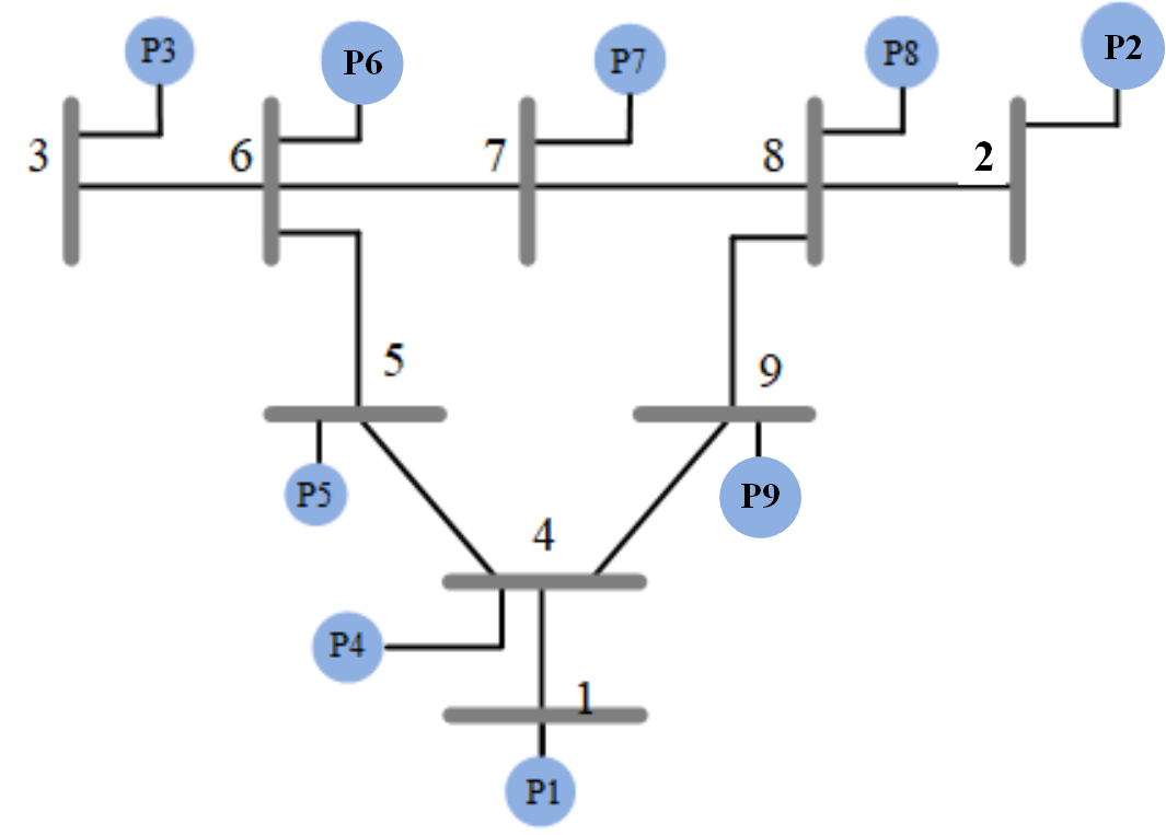
Figure 4: IEEE-9-bus system with 9 prosumers (P1-P9).

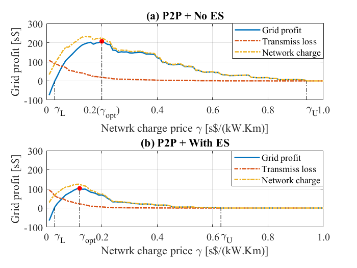
Figure 5: Grid profit w.r.t. network charge price $\gamma$ for IEEE 9-bus system: (a) P2P + No ES. (b) P2P + With ES. ($\gamma_{\rm L}$: minimum network charge price for the grid to attribute transmission loss. $\gamma_{\rm opt}$: optimal network charge price for maximum grid profit. $\gamma_{\rm U}$: maximum network charge price that the prosumers would take.)

IV-B IEEE 9-bus system

We first use the small-scale IEEE 9-bus system with 9 prosumers shown in Fig. 4 to evaluate the proposed optimal network charge model. By solving the ($P$), we can obtain the optimal network charge price $\gamma_{\rm opt}=0.2$ $\mathrm{s}\$\mathrm{/}\mathrm{(}\mathrm{k}\mathrm{W}\cdot\mathrm{k}\mathrm{m}\mathrm{)}$ (No ES) and $\gamma_{\rm opt}=0.12$$\mathrm{s}\$\mathrm{/}\mathrm{(}\mathrm{k}\mathrm{W}\cdot\mathrm{k}\mathrm{m}\mathrm{)}$ (With ES). To verify the solution accuracy, we compare the obtained solutions with that identified from simulating the range of network charge price $\gamma\in[0,1]$$\mathrm{s}\$\mathrm{/}\mathrm{(}\mathrm{k}\mathrm{W}\cdot\mathrm{k}\mathrm{m}\mathrm{)}$ with an incremental of $\Delta\gamma=0.01$ $\mathrm{s}\$\mathrm{/}\mathrm{(}\mathrm{k}\mathrm{W}\cdot\mathrm{k}\mathrm{m}\mathrm{)}$. For each simulated network charge price, we evaluate the grid profit, network charge, and transmission loss defined in (${\rm P}_{U}$) and display their changes w.r.t. the network charge price in Fig. 5. From the results, the optimal network charge price can be identified where the grid profit is maximized, which are $\gamma_{\rm opt}=0.2$ $\mathrm{s}\$\mathrm{/}\mathrm{(}\mathrm{k}\mathrm{W}\cdot\mathrm{k}\mathrm{m}\mathrm{)}$ (No ES) and $\gamma_{\rm opt}=0.12$$\mathrm{s}\$\mathrm{/}\mathrm{(}\mathrm{k}\mathrm{W}\cdot\mathrm{k}\mathrm{m}\mathrm{)}$ (With ES) corresponding well to the obtained solutions. This demonstrates the effectiveness of the proposed solution method. By further examining the simulation results, we can draw the following main conclusions.

IV-B1 The network charge model admits an equilibrium network charge price

From Fig. 5 (a) (No ES) and 5 (b) (With ES), we observe that the grid profit first approximately increases and begins to drop after reaching the optimal network charge price $\gamma_{\rm opt}$ with the maximum grid profit. Since for any given network charge price $\gamma$, there exists an optimal energy management strategy for the prosumers (i.e., there exists an optimal solution for the lower level problem (${\rm P}_{L}$)), we imply that $\gamma_{\rm opt}$ is the equilibrium network charge price. This demonstrates the existence of equilibrium for the proposed Stackelberg game, which is in line with Theorem 1.

Besides, we can imply from the results that there exists a minimal network charge price for the grid operator to attribute the transmission loss. Such minimal network charge price occurs where the network charge revenue equals the transmission loss (i.e., the grid operator has zero profit). Specifically, the minimal network charge price is $\gamma_{\rm L}=0.03$\mathrm{s}\$\mathrm{/}\mathrm{(}\mathrm{k}\mathrm{W}\cdot\mathrm{k}\mathrm{m}\mathrm{)}$$ both with and without ES for the tested case. In addition, we note that there also exists a maximal network charge price that the prosumers would take, which are $\gamma_{\rm U}=0.94$$\mathrm{s}\$\mathrm{/}\mathrm{(}\mathrm{k}\mathrm{W}\cdot\mathrm{k}\mathrm{m}\mathrm{)}$ (No ES) and $\gamma_{\rm U}=0.6$\mathrm{s}\$\mathrm{/}\mathrm{(}\mathrm{k}\mathrm{W}\cdot\mathrm{k}\mathrm{m}\mathrm{)}$$ (With ES) for the tested case. When the network charge price exceeds the maximum price, we observe that no transaction happens in the P2P market. We note that when the prosumers have ES, they would take lower network charge price. This is reasonable as the prosumers can use the ES to shift surplus renewable generation for future use in addition to trade in the P2P market. This can be perceived from Fig 6 which shows the total P2P trades in the P2P market w.r.t. the network charge price both with and without ES. We note that less trades will be made when the prosumers have ES than that of No ES for any specific network charge price. Moreover, the total trades drop faster w.r.t. the increase of network charge price when the prosumers have ES. This implies that the deployment of ES will make the prosumers more sensitive to the network charge price and impact the optimal network charge price.

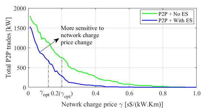
Figure 6: Total P2P trades w.r.t. network charge price $\gamma$ for IEEE 9-bus system ($\gamma_{\rm opt}$: optimal network charge price).

IV-B2 The network charge can benefit both the grid operator and the prosumers

From the above results, we conclude that the proposed optimal network charge can provide positive profit to the grid operator. This implies that the grid operator can benefit from empowering P2P energy trading. An interesting question to ask is how the economic benefit of P2P is shared by the grid operator and the prosumers with the proposed network charge mechanism. To answer that question, we use No P2P as the base and define the increased profit for the grid operator and the prosumers as the benefit harnessed from a specific P2P market. We compare the benefit of the two stakeholders with Optimal P2P and Free P2P. For Optimal P2P, we impose the obtained optimal network charge price $\gamma_{\rm opt}=0.2$ $\mathrm{s}\$\mathrm{/}\mathrm{(}\mathrm{k}\mathrm{W}\cdot\mathrm{k}\mathrm{m}\mathrm{)}$ (No ES) and $\gamma_{\rm opt}=0.1$$\mathrm{s}\$\mathrm{/}\mathrm{(}\mathrm{k}\mathrm{W}\cdot\mathrm{k}\mathrm{m}\mathrm{)}$. For Free P2P, we set a sufficiently small network charge price $\gamma=1e-7$$\mathrm{s}\$\mathrm{/}\mathrm{(}\mathrm{k}\mathrm{W}\cdot\mathrm{k}\mathrm{m}\mathrm{)}$ to ensure the uniqueness of solution as mentioned. We evaluate the benefit of grid operator and prosumers for each time period and display the results over the 24 periods in Fig. 7 (No ES) and Fig. 8 (With ES). We note that when there is no network charge (i.e., Free P2P and Free P2P + ES), the prosumers can gain considerable benefit from P2P transaction. Whereas the grid operator will have to undertake the transmission loss which are in total 116.94s$ (No ES) and 103.38s$ (With ES). Comparatively, the proposed optimal network charge (i.e., Optimal P2P, Optimal P2P + ES) can provide positive benefit to both the grid operator and the prosumers, i.e., 206.77s$ vs. 158.67s$ (No ES) and 103.01s$ vs. 76.50s$ (With ES). We therefore imply that the optimal (equilibrium) network charge price that maximizes the grid profit also secures the prosumers’ profit. Moreover, the benefit of P2P is almost equally shared by the grid operator and the prosumers (i.e., 57.38% vs. 42.6%).

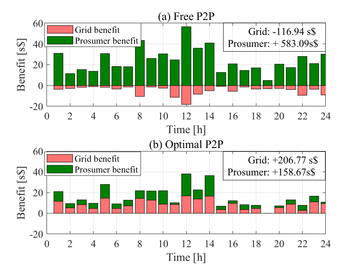
Figure 7: Benefit of the grid operator and prosumers with Optimal P2P and Free P2P for IEEE 9-bus system (using No P2P as benchmark).

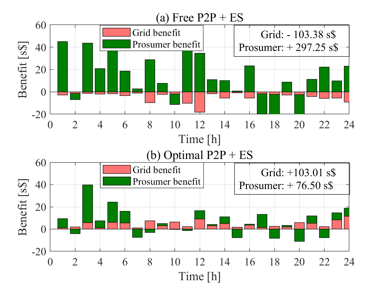
Figure 8: Benefit of the grid operator and prosumers with Free P2P + ES and Optimal P2P + ES for IEEE 9-bus system (using No P2P as benchmark).

IV-B3 The network charge provides near-optimal social welfare

Social welfare is one of the most important measures to be considered for market design. For the concerned P2P market involving the grid operator and the prosumers, the social welfare refers to the sum profit of grid operator and prosumers (i.e., social profit) and defined as ${\rm Social~{}profit}={\textstyle\sum}_{t}{\textstyle\sum}_{i}U_{i,t}(\mathcal{P}_{i,t})-\rho{\textstyle\sum}_{t}{\textstyle\sum}_{(i,j)\in\mathcal{L}}b_{ij}(\theta_{i,t}-\theta_{j,t})^{2}$. In this part, we study the social profit yield by the proposed network charge model. To identify the social optimality gap, we compare Optimal P2P with Social P2P. We evaluate the social profit for each time period with Optimal P2P and Social P2P, and display the results over the 24 periods in Fig. 9 (a) (No ES) and Fig. 9 (b) (With ES). To identify the social optimality gap, we fill the difference of social profit curves with Optimal P2P and Social P2P in blue. Note that the positive area can be interpreted as the social optimality gap. From the results, we conclude that the social optimality gap is about 4.70% (No ES) and $1.32\%$ (With ES). To be noted, though we observe a larger shaded area for the case with ES (see Fig. 9 (b)), the accumulated positive area is quite small. This implies that the proposed network charge mechanism can provide near-optimal social welfare.

We further study how the social profit is affected by the network charge price. Similarly, we simulate the range of network charge price $\gamma\in[0,1]$$\mathrm{s}\$\mathrm{/}\mathrm{(}\mathrm{k}\mathrm{W}\cdot\mathrm{k}\mathrm{m}\mathrm{)}$ with an incremental of $\Delta\gamma=0.01$ $\mathrm{s}\$\mathrm{/}\mathrm{(}\mathrm{k}\mathrm{W}\cdot\mathrm{k}\mathrm{m}\mathrm{)}$. For each simulated network charge price, we evaluate the total social profit over the 24 periods. As shown in Fig. 10, we observe that the social profit first increases w.r.t. the network charge and begins to drop after the social optima is reached. Besides, we note that though the obtained optimal network charge price does not coincide with the social optima, the social optimality gap is quite small, which are only $4.70\%$ and $1.32\%$ (With ES) as discussed.

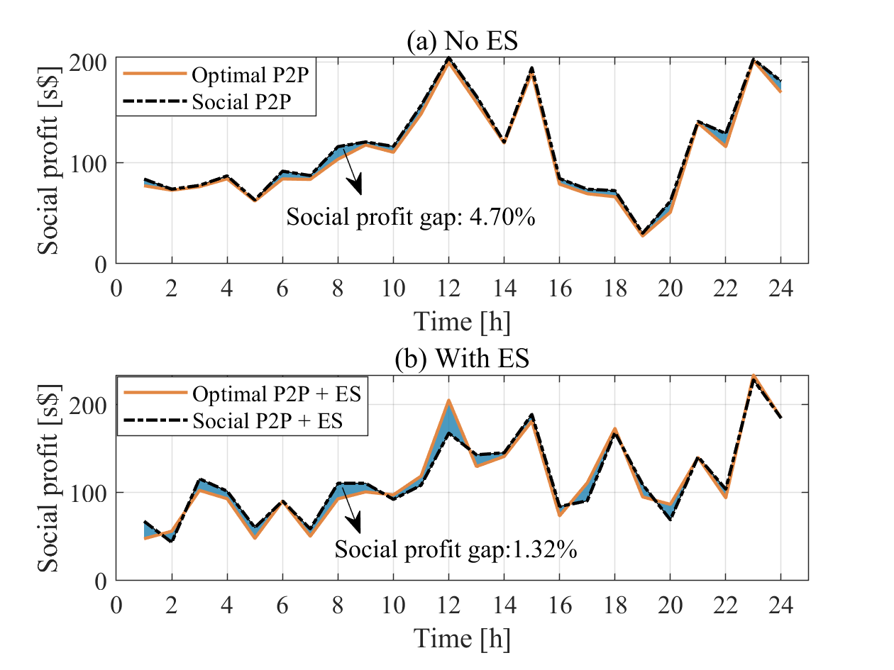
Figure 9: Social profit for each time period for IEEE-9-bus system: (a) No ES. (b) With ES. (Positive shaded area represents the social profit loss of Optimal P2P compared with Social P2P).

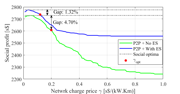
Figure 10: Social profit w.r.t. network charge price for IEEE-9-bus system. (P2P + With ES: social optimality gap 1.32%. P2P + No ES: social optimality gap 4.70%.)

IV-B4 The network charge favors localized transaction and curbs long distancing transaction

In this part, we study how the proposed network charge shapes the P2P markets. We compare Optimal P2P with Free P2P both with and without ES on the prosumer side. For each market, we calculate the aggregated transaction (in $\mathrm{kW}$) for the trading peers over the 24 periods and visualize the transaction in Fig. 11. The circles with IDs indicate the prosumers and the line thickness represents the amounts of P2P transaction. We observe that the network charge has an obvious impact on the behaviors of prosumers in the P2P markets. Specifically, by comparing Fig. 11 (a) (No ES) and Fig. 11 (b) (With ES), we notice that the network charge dose not affect the transaction between the prosumers in close proximity (e.g., 3-6, 7-8, 2-8, 1-4) but obviously discourages the long distancing transaction (e.g., 4-6, 1-6, 1-9). This is reasonable as the network charge counts on the electrical distance. Therefore, the proposed network charge model favors localized transaction and curbs the long distancing transaction. This makes sense considering the transmission losses related to the long distancing transaction. For the case with ES, we can draw the similar conclusion from Fig. 11 (a) (No ES) and Fig. 11 (b) (With ES).

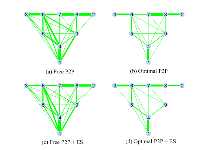
Figure 11: Total P2P trades of 24 periods across the prosumers for IEEE 9-bus system (line thickness represents the amounts of transaction).

IV-C IEEE 39-bus, 57-bus and 118-bus systems

TABLE IV: Outcomes of different P2P markets

System	Market	Grid-wise			Prosumer-wise		System-wise
		Transmission loss	Network charge	Grid profit	Prosumer profit	Total transaction	Social profit
		$\times 10^{2}$[s$]	$\times 10^{2}$[s$]	$\times 10^{2}$[s$]	$\times 10^{2}$[s$]	$\times 10^{2}$[$\mathrm{kW}\text{\,}\mathrm{h}$]	$\times 10^{2}$[s$]
9-bus	No P2P	0	0	0	22.42	0	22.42
	Free P2P	1.17	0	-1.17	28.25	17.43	27.10
	Social P2P	–	–	–	–	–	27.35
	Optimal P2P	0.19	2.26	2.07	24.00	7.82	26.08
	No P2P+ES	0	0	0	25.57	0	25.57
	Free P2P+ES	1.03	0	-1.03	28.54	15.57	27.51
	Social P2P+ES	–	–	–	–	–	27.87
	Optimal P2P+ES	0.28	1.22	0.94	26.56	7.64	27.50
39-bus	No P2P	0	0	0	110.86	0	110.86
	Free P2P	3.27	0	-3.27	151.03	112.64	147.76
	Social P2P	–	–	–	–	–	148.15
	Optimal P2P	0.55	14.79	14.24	123.44	52.33	137.68
	No P2P+ES	0	0	0	124.69	0	124.69
	Free P2P + ES	2.62	0	-2.62	154.38	107.69	151.76
	Social P2P + ES	–	–	–	–	–	152.18
	Optimal P2P+ES	0.60	11.26	10.65	134.07	45.17	144.73
57-bus	No P2P	0	0	0	191.63	–	191.63
	Free P2P	65.52	0	-65.52	26.20	185.61	196.53
	Social P2P	–	–	–	–	–	232.05
	Optimal P2P	4.72	22.40	17.68	205.94	61.16	223.61
	No P2P + ES	0	0	0	212.50	0	212.50
	Free P2P + ES	66.20	0	-66.20	272.92	177.23	206.75
	Social P2P + ES	–	–	–	–	–	240.19
	Optimal P2P+ES	5.39	18.49	13.10	222.52	52.45	235.62
118-bus	No P2P	0	0	0	427.68	0	427.68
	Free P2P	111.20	0	-111.20	567.38	367.09	455.64
	Social P2P	–	–	–	–	–	530.84
	Optimal P2P	5.33	46.97	41.63	46.76	149.59	509.18
	No P2P + ES	0	0	0	474.84	0	474.84
	Free P2P + ES	177.47	0	-177.47	603.83	391.05	426.35
	Social P2P + ES	–	–	–	–	–	557.79
	Optimal P2P + ES	5.46	37.43	31.97	505.38	128.27	537.35

We further examine the performance of the proposed network charge mechanism by simulating the IEEE 39-bus, 57-bus, and 118-bus systems. We follow the same simulation set-ups in Section IV-A and compare the different markets in TABLE III. We report the results for different markets and bus systems in TABLE IV. Particularly, we group the results by Grid-wise, Prosumer-wise and System-wise. For Grid-wise, we study the total transmission loss, network charge revenue and the grid profit. For Prosumer-wise, we are concerned with the total prosumer profit and total P2P transaction. For System-wise, we evaluate the social profit (i.e., grid operator profit plus prosumers’ profit). Note that the results for IEEE 9-bus system are also included for completeness. The results associated with Optimal P2P and Optimal P2P + ES have been highlighted in bold as our main focus. Overall, for the larger electrical networks, we can draw similar results in Section IV-B.

Specially, the proposed optimal network charge can provide positive profit both to the power grid and the prosumers as with Optimal P2P and Optimal P2P + ES reported in TABLE IV. Whereas Free P2P and Free P2P + ES only favor the prosumers with considerable profit increase over No P2P and will displease the power grid operator considering the uncovered transmission loss (i.e., negative profit for the grid operator). This implies that the network charge is necessary to enable the successful deployment of P2P market in the existing power system from the perspective of economic benefit.

Besides, we can conclude that the proposed network charge is favorable considering the benefit of P2P shared by the grid operator and the prosumers. Similarly, using No ES as the benchmark, we define the profit increase of the grid operator and the prosumers as the benefit. Based on the results in TABLE IV, we have the report regarding the benefit of grid operator and the prosumers in Fig. 12 (a) (No ES) and 12 (b) (With ES). Notably, we see that the grid operator and the prosumers achieve almost equal benefit from the P2P market with all cases. Specifically, the benefit for the prosumers and grid operator are about 49.0% vs. 51.0% (No ES) and 48.4% vs. 51.6% (With ES) for the tested IEEE-118 bus systems. This makes sense considering the balance of the P2P market.

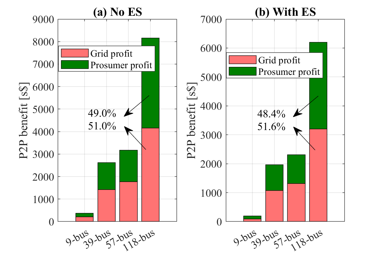
Figure 12: Benefit of grid operator and the prosumers with Optimal P2P: (a) No ES. (b) With ES. (using No P2P as benchmark)

In addition, we conclude that the network charge can be used to shape the P2P markets. For the tested bus systems, we compare the P2P transaction of Free P2P and Optimal P2P both with and without ES. Similarly, we visualize the total transaction over the 24 periods for the trading peers in Fig. 14 (39-bus), 15 (57-bus), 16 (118-bus). The circles with IDs indicate prosumers located at the buses and line thickness represents the amounts of transactions. We note that the imposed network charge has an obvious impact on the energy trading behaviors of prosumers in the P2P market. When there is no network charge and the grid operator has no manipulation on the P2P market, the prosumers could trade regardless of the electrical distances, leading to massive long distancing trades. The could be problematic considering the high transmission loss and the possible network violations taken by the grid operator. Comparatively, the proposed network charge favors localized transaction and discourages long distancing transaction, yielding much lower transmission loss as reported in TABLE IV (see Column 3). More importantly, the network charge is necessary for the grid operator to ensure the network constraints.

Last but not the least, we conclude that the proposed network charge favors social welfare. By examining the System-wise performance indicated by social profit in TABLE IV (Column 8), we notice that P2P transaction (i.e., Optimal P2P, Free P2P and Social P2P) favors social profit over No P2P. More notably, we find that Optimal P2P and Optimal P2P + ES provide near-optimal social profit indicated by Social P2P. Specifically, the overall social optimality gap is less than 7% (No ES) and less than 5% (With ES) with Optimal P2P as reported in Fig. 13,

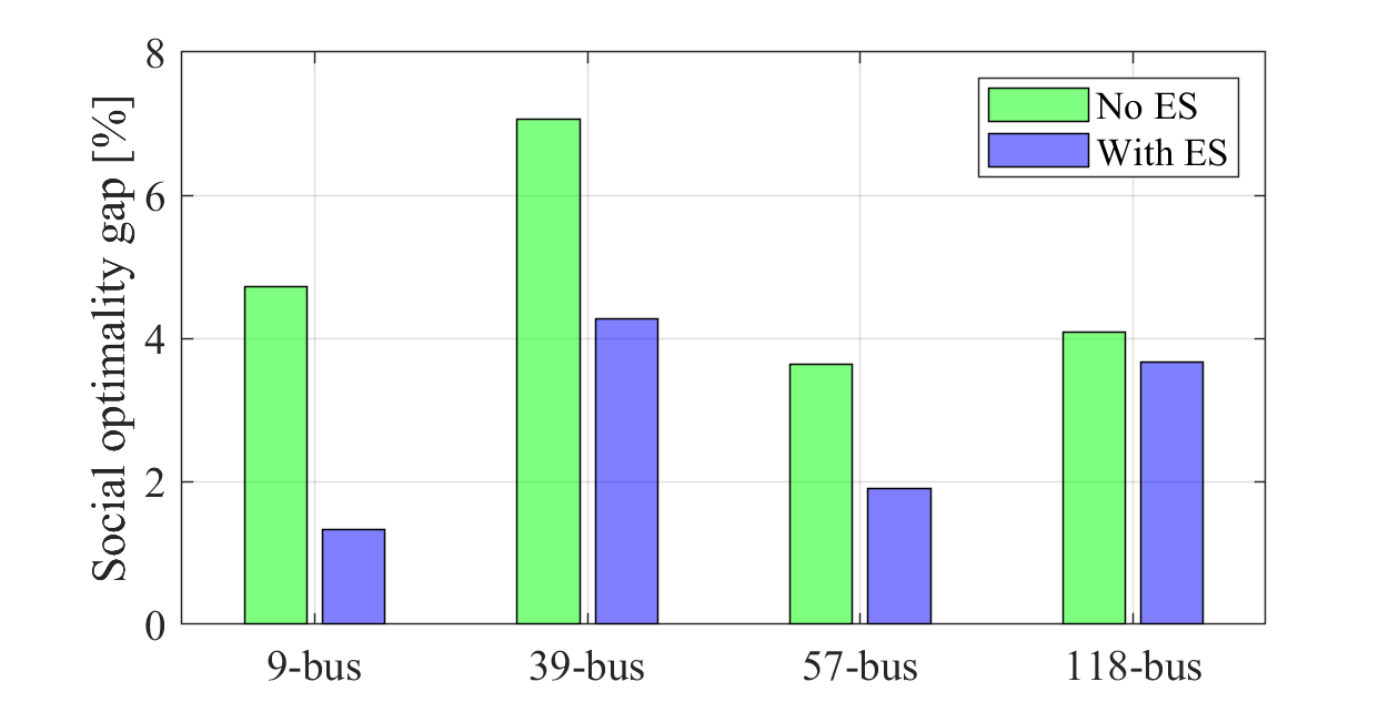
Figure 13: Social optimality gap of Optimal P2P.

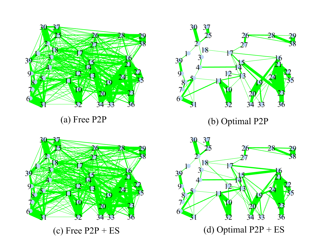
Figure 14: Total P2P trades of 24 periods across the prosumers for IEEE 39-bus system (line thickness represents the amount of transaction).

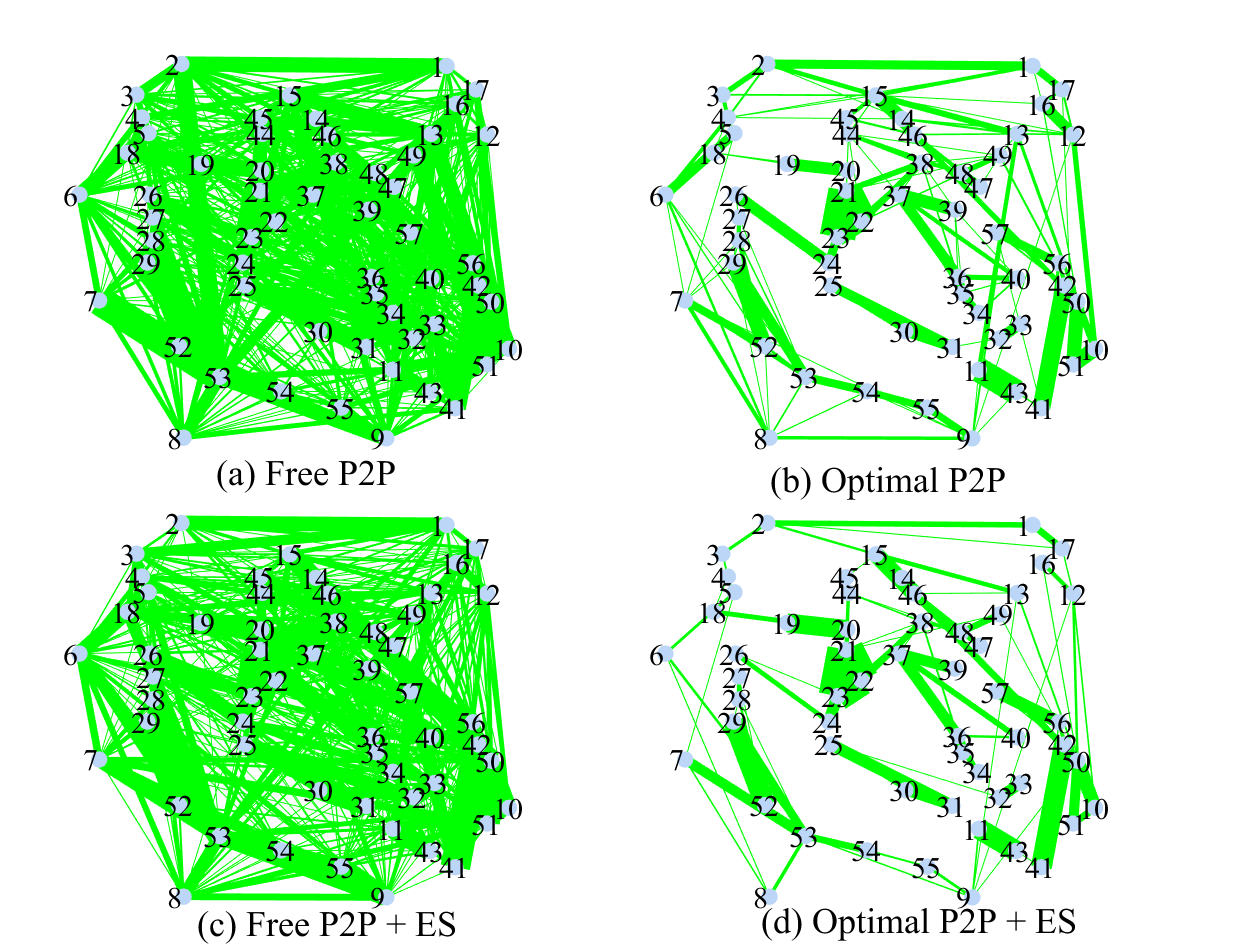
Figure 15: Total P2P trades of 24 periods across the prosumers for IEEE 57-bus system (line thickness represents the amount of transaction).

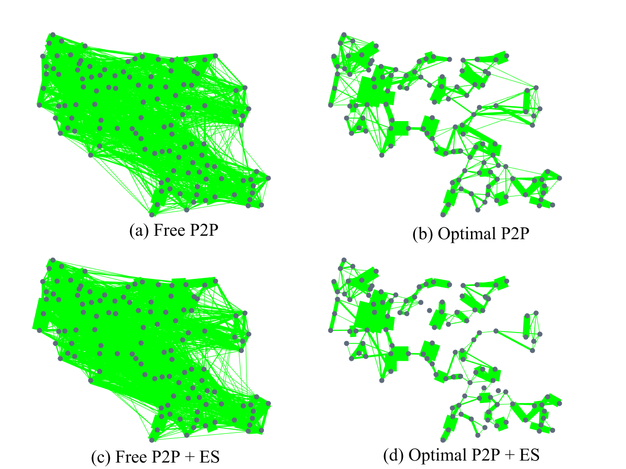
Figure 16: Total P2P trades of 24 periods across the prosumers for IEEE 118-bus system (line thickness represents the amount of transaction).

V Conclusion and Future Works

This paper discussed the integration of the P2P market scheme into the existing power systems from the perspective of network charge design. We used network charge as a means for the grid operator to attribute grid-related cost (i.e., transmission loss) and ensure network constraints for empowering P2P transaction. We characterized the interaction between the power grid operator and the prosumers in a P2P market as a Stackelberg game. The grid operator first decides on the optimal network charge price to trade off the network charge revenue and the transmission loss considering the network constraints, and then the prosumers optimize their energy management (i.e., energy consuming, storing and trading) for maximum economic benefit. We proved the Stackelberg game admits an equilibrium network charge price. Besides, we proposed a solution method to obtain the equilibrium network charge price by converting the bi-level optimization problem into a single-level optimization problem. By simulating the IEEE bus systems, we demonstrated that the proposed network charge mechanism can benefit both the grid operator and the prosumers and achieve near-optimal social welfare. In addition, we found that the presence of ES on prosumer side will make the prosumers more sensitive to the network charge price increase.

In this paper, we have studied the optimal network charge with deterministic supply and demand and found that the network charge is effective in shaping the behaviors of prosumers in a P2P market. Some future works along this line include: 1) designing optimal network charge price considering the uncertainties of prosumer supply and demand; 2) using the network charge as a tool to achieve demand response.

References

- [1] IEA, “Distributed energy resources for net zero: An asset or a hassle to the electricity grid?.” https://www.iea.org/commentaries/distributed-energy-resources-for-net-zero-an-asset-or-a-hassle-to-the-electricity-grid, 2021. Accessed: 2022-04-24.
- [2] Y. Yang, Q.-S. Jia, G. Deconinck, X. Guan, Z. Qiu, and Z. Hu, “Distributed coordination of ev charging with renewable energy in a microgrid of buildings,” IEEE Transactions on Smart Grid, vol. 9, no. 6, pp. 6253–6264, 2017.
- [3] Y. Yang, Q.-S. Jia, X. Guan, X. Zhang, Z. Qiu, and G. Deconinck, “Decentralized ev-based charging optimization with building integrated wind energy,” IEEE Transactions on Automation Science and Engineering, vol. 16, no. 3, pp. 1002–1017, 2018.
- [4] Y. Yang, U. Agwan, G. Hu, and C. J. Spanos, “Selling renewable utilization service to consumers via cloud energy storage,” arXiv preprint arXiv:2012.14650, 2020.
- [5] T. Morstyn, N. Farrell, S. J. Darby, and M. D. McCulloch, “Using peer-to-peer energy-trading platforms to incentivize prosumers to form federated power plants,” Nature Energy, vol. 3, no. 2, pp. 94–101, 2018.
- [6] C. Zhang, J. Wu, Y. Zhou, M. Cheng, and C. Long, “Peer-to-peer energy trading in a microgrid,” Applied Energy, vol. 220, pp. 1–12, 2018.
- [7] Y. Chen, W. Wei, H. Wang, Q. Zhou, and J. P. Catalão, “An energy sharing mechanism achieving the same flexibility as centralized dispatch,” IEEE Transactions on Smart Grid, vol. 12, no. 4, pp. 3379–3389, 2021.
- [8] Y. Chen, Y. Yang, and X. Xu, “Towards transactive energy: An analysis of information-related practical issues,” Energy Conversion and Economics, vol. 3, no. 3, pp. 112–121, 2022.
- [9] W. Tushar, C. Yuen, H. Mohsenian-Rad, T. Saha, H. V. Poor, and K. L. Wood, “Transforming energy networks via peer-to-peer energy trading: The potential of game-theoretic approaches,” IEEE Signal Processing Magazine, vol. 35, no. 4, pp. 90–111, 2018.
- [10] W. Tushar, T. K. Saha, C. Yuen, T. Morstyn, H. V. Poor, R. Bean, et al., “Grid influenced peer-to-peer energy trading,” IEEE Transactions on Smart Grid, vol. 11, no. 2, pp. 1407–1418, 2019.
- [11] T. Baroche, F. Moret, and P. Pinson, “Prosumer markets: A unified formulation,” in 2019 IEEE Milan PowerTech, pp. 1–6, IEEE, 2019.
- [12] S. Cui, Y.-W. Wang, and J.-W. Xiao, “Peer-to-peer energy sharing among smart energy buildings by distributed transaction,” IEEE Transactions on Smart Grid, vol. 10, no. 6, pp. 6491–6501, 2019.
- [13] Y. Yang, G. Hu, and C. J. Spanos, “Optimal sharing and fair cost allocation of community energy storage,” IEEE Transactions on Smart Grid, vol. 12, no. 5, pp. 4185–4194, 2021.
- [14] D. Teixeira, L. Gomes, and Z. Vale, “Single-unit and multi-unit auction framework for peer-to-peer transactions,” International Journal of Electrical Power & Energy Systems, vol. 133, p. 107235, 2021.
- [15] T. Morstyn, A. Teytelboym, and M. D. McCulloch, “Bilateral contract networks for peer-to-peer energy trading,” IEEE Transactions on Smart Grid, vol. 10, no. 2, pp. 2026–2035, 2018.
- [16] J. Kim and Y. Dvorkin, “A p2p-dominant distribution system architecture,” IEEE Transactions on Power Systems, vol. 35, no. 4, pp. 2716–2725, 2019.
- [17] T. Sousa, T. Soares, P. Pinson, F. Moret, T. Baroche, and E. Sorin, “Peer-to-peer and community-based markets: A comprehensive review,” Renewable and Sustainable Energy Reviews, vol. 104, pp. 367–378, 2019.
- [18] M. Khorasany, Y. Mishra, and G. Ledwich, “Market framework for local energy trading: A review of potential designs and market clearing approaches,” IET Generation, Transmission & Distribution, vol. 12, no. 22, pp. 5899–5908, 2018.
- [19] M. R. Hamouda, M. E. Nassar, and M. Salama, “A novel energy trading framework using adapted blockchain technology,” IEEE Transactions on Smart Grid, vol. 12, no. 3, pp. 2165–2175, 2020.
- [20] A. Esmat, M. de Vos, Y. Ghiassi-Farrokhfal, P. Palensky, and D. Epema, “A novel decentralized platform for peer-to-peer energy trading market with blockchain technology,” Applied Energy, vol. 282, p. 116123, 2021.
- [21] W. Tushar, T. K. Saha, C. Yuen, D. Smith, and H. V. Poor, “Peer-to-peer trading in electricity networks: An overview,” IEEE Transactions on Smart Grid, vol. 11, no. 4, pp. 3185–3200, 2020.
- [22] T. Baroche, P. Pinson, R. L. G. Latimier, and H. B. Ahmed, “Exogenous cost allocation in peer-to-peer electricity markets,” IEEE Transactions on Power Systems, vol. 34, no. 4, pp. 2553–2564, 2019.
- [23] J. Guerrero, A. C. Chapman, and G. Verbič, “Decentralized p2p energy trading under network constraints in a low-voltage network,” IEEE Transactions on Smart Grid, vol. 10, no. 5, pp. 5163–5173, 2018.
- [24] A. Paudel, L. Sampath, J. Yang, and H. B. Gooi, “Peer-to-peer energy trading in smart grid considering power losses and network fees,” IEEE Transactions on Smart Grid, vol. 11, no. 6, pp. 4727–4737, 2020.
- [25] P. Cuffe and A. Keane, “Visualizing the electrical structure of power systems,” IEEE Systems Journal, vol. 11, no. 3, pp. 1810–1821, 2015.
- [26] R. D. Christie, B. F. Wollenberg, and I. Wangensteen, “Transmission management in the deregulated environment,” Proceedings of the IEEE, vol. 88, no. 2, pp. 170–195, 2000.
- [27] L. Ding, G. Y. Yin, W. X. Zheng, Q.-L. Han, et al., “Distributed energy management for smart grids with an event-triggered communication scheme,” IEEE Transactions on Control Systems Technology, vol. 27, no. 5, pp. 1950–1961, 2018.
- [28] M. Farivar and S. H. Low, “Branch flow model: Relaxations and convexification—part i,” IEEE Transactions on Power Systems, vol. 28, no. 3, pp. 2554–2564, 2013.
- [29] R. Rigo-Mariani and V. Vai, “An iterative linear distflow for dynamic optimization in distributed generation planning studies,” International Journal of Electrical Power & Energy Systems, vol. 138, p. 107936, 2022.
- [30] J. Jo and J. Park, “Demand-side management with shared energy storage system in smart grid,” IEEE Transactions on Smart Grid, vol. 11, no. 5, pp. 4466–4476, 2020.
- [31] F. Rey, X. Zhang, S. Merkli, V. Agliati, M. Kamgarpour, and J. Lygeros, “Strengthening the group: Aggregated frequency reserve bidding with admm,” IEEE Transactions on Smart Grid, vol. 10, no. 4, pp. 3860–3869, 2018.
- [32] Z. Xu, L. Guo, Y. Gao, M. Hussain, and P. Cheng, “Real-time pricing of smart grid based on piece-wise linear functions:,” Journal of Systems Science and Information, vol. 7, no. 4, pp. 295–316, 2019.
- [33] L. Wu, “A tighter piecewise linear approximation of quadratic cost curves for unit commitment problems,” IEEE Transactions on Power Systems, vol. 26, no. 4, pp. 2581–2583, 2011.
- [34] S. Dempe and A. Zemkoho, Bilevel optimization. Springer, 2020.
- [35] S. Boyd, S. P. Boyd, and L. Vandenberghe, Convex optimization. Cambridge university press, 2004.
- [36] C. Feng, Z. Li, M. Shahidehpour, F. Wen, and Q. Li, “Stackelberg game based transactive pricing for optimal demand response in power distribution systems,” International Journal of Electrical Power & Energy Systems, vol. 118, p. 105764, 2020.
- [37] S. P. Bradley, A. C. Hax, and T. L. Magnanti, Applied Mathematical Programming. MA: Addison-Wesley Publishing Company, 1977.
- [38] “Openei.” https://openei.org/datasets/files/961/pub/. Accessed: 2021-07-31.
- [39] N. Measurement and I. D. C. (MIDC). https://midcdmz.nrel.gov/apps/daily.pl?site=NWTC&start=20010824&yr=2020&mo=1&dy=28. Accessed: 2021-07-31.