Frequency Domain-Based Detection of Generated Audio

Abstract

Attackers may manipulate audio with the intent of presenting falsified reports, changing an opinion of a public figure, and winning influence and power. The prevalence of inauthentic multimedia continues to rise, so it is imperative to develop a set of tools that determines the legitimacy of media. We present a method that analyzes audio signals to determine whether they contain real human voices or fake human voices (i.e., voices generated by neural acoustic and waveform models). Instead of analyzing the audio signals directly, the proposed approach converts the audio signals into spectrogram images displaying frequency, intensity, and temporal content and evaluates them with a Convolutional Neural Network (CNN). Trained on both genuine human voice signals and synthesized voice signals, we show our approach achieves high accuracy on this classification task.

I. Introduction

Synthesized media can be generated for multiple different modalities, including text, images, videos, and audio. Technological advancements enable people to generate manipulated or false multimedia content relatively easily. Because generating false content is so accessible, the quantity of synthesized media increases exponentially daily [1]. Fabricated content has been used for years for entertainment purposes, such as in movies or comedic segments. However, it also has the potential to be introduced for nefarious purposes.

Genuine Audio Signal

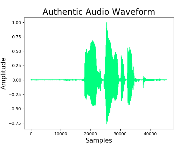
(a)

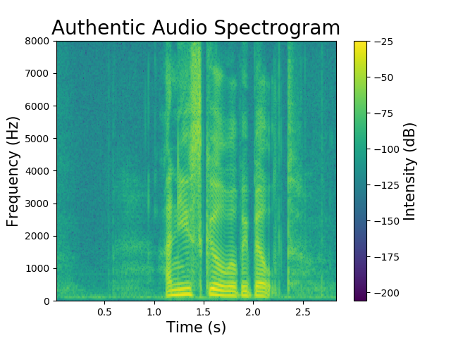
(b)

Synthesized Audio Signal

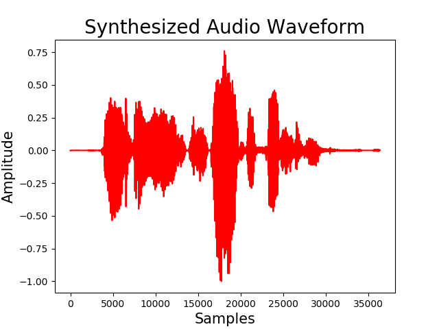
(c)

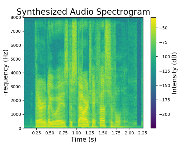
(d)

Figure 1: Left column: Audio signals in the time domain, where green indicates a genuine audio signal spoken by a human and red indicates a synthesized audio signal. Right column: Spectrograms generated from the time domain audio signals, which are used by the CNN to determine audio authenticity.

Society has experienced only the tip of the iceberg in terms of consequences of synthesized media. The true harm of DeepFakes and other falsified content has not yet been realized. This ticking time bomb could wreck havoc throughout the world with impact on a personal, societal, and global level [2].

Audio authentication is necessary for speaker verification. If audio is synthesized to impersonate someone successfully, an adversary may access personal devices with confidential information, such as banking details and medical records. Furthermore, fabricated audio could be used in the audio tracks of DeepFake videos.

In this paper, we consider an audio authentication task. The reason for this is twofold. First, there are cases in which the only medium available is audio, such as in a speaker verification task. Second, there are cases in which multiple types of data are available for analysis, such as a DeepFake detection task, which would benefit from a multi-modal analysis that includes fake audio detection. Our method examines audio signals in the frequency domain in the form of spectrograms, as shown in Figure 1.

A spectrogram is a visualization technique for audio signals. It shows the relationship between time, frequency, and intensity (or “loudness”) of an audio signal – all in the same graph. Time increases from left to right along the horizontal axis, while frequency increases from bottom to top along the vertical axis. Colors densely fill the middle of the graph and indicate the strength of a signal over time at different frequencies. Much like a heat map, brighter colors depict greater strength. We treat these spectrograms as images and analyze them using Deep Learning techniques to determine whether an audio track is genuine or synthesized, as shown in Figure 2.

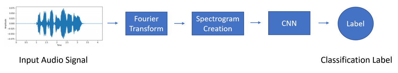
(a)

Figure 2: Proposed Method. The proposed approach transforms audio signals in the time domain into spectrogram “images”, which are used as inputs to the CNN. Then, the CNN produces a classification label indicating whether the signal under analysis is authentic or synthesized.

II. Related Work

Developing methods to verify multimedia is an ongoing research effort. Previous work includes analysis of audio content [3], visual content [4] [5] [6] [7], metadata [8], and combinations of these modalities [9].

A. Spoofing Attacks

For the audio modality specifically, spoofing attacks fall into three main categories: voice conversion (VC), speech synthesis (SS), and replay attacks. Voice conversion refers to the process of transforming an already existing speech signal into the style of another speaker, so that it sounds as if a new speaker is saying exactly what the original speaker said. Speech synthesis refers to methods in which new audio signals are generated from scratch. For example, converting written text into spoken speech is one method to achieve speech synthesis. Finally, replay attacks refer to spoofing methods in which the original speaker and desired speech signal are recorded. Then, this speech signal is played back to an audio-capturing device, which is fooled into believing the replayed audio signal is the desired speaker in real-time. Some research efforts, such as [3], focus on replay attacks specifically. On the other hand, we focus solely on voice conversion and speech synthesis attacks, which consist of synthetically generated audio signals.

B. Audio Features

Digital signal processing offers many different methods to extract features to analyze audio signals. Arguably the most famous method for signal analysis is the Fourier Transform (FT) and its subsidiaries (e.g., Discrete Fourier Transform (DFT)), which deconstruct a function of time into its constituent frequencies.

Many techniques build upon the foundation of the Fourier Transform. Constant Q Cepstral Coefficients (CQCCs) are derived by converting a signal from time domain to frequency domain with the Fourier Transform, spacing the spectral amplitudes logarithmically, and then converting the amplitudes to the quefrency domain with a time scale [10].

Mel Frequency Cepstral Coefficients (MFCCs) are also based on the Fourier Transform. In order to compute MFCCs, the Fourier Transform is applied to time domain audio signals, and the powers of the resulting spectrum are mapped onto the mel scale [11]. The mel scale describes how humans perceive tones and pitches. It reflects humans’ sensitivity to different frequencies [12]. Next, the logarithmic scale is applied to the powers at each of the mel frequencies in preparation to compute the Discrete Cosine Transform (DCT) [13] of the mel log powers. Finally, the amplitudes of the result of the DCT constitute the MFCCs [14].

Besides enabling the computation of feature coefficients, the Fourier Transform may be used to construct visual representations of signals. Nowadays, spectrogram generation is a digital process which involves sampling a signal in the time domain, dividing the signal into smaller segments, and applying the Fourier Transform to each segment to calculate the magnitude of the frequency spectrum for each segment. Through this process, a segment corresponding to a specific moment in time is transformed into a sequence of spectrum magnitude values. To construct a graph of these values, the sequence is oriented as a vertical line and color coded according to magnitude, creating a vertical line of “pixels.” These pixel lines are concatenated side-by-side in order of increasing time index to construct a spectrogram “image.”

C. Audio Authentication Approaches

Current audio authentication methods utilize the aforementioned features to determine whether an audio signal is real or fake. They first estimate the desired audio features from the time domain signal and then use them as inputs to a Deep Learning system. For example,  [15] uses CQCCs and MFCCs as inputs to a standard feedforward Multilayer Perceptron Network (MLP) and ResNet-based Convolutional Neural Network (CNN).  [3] investigates CQCCs and MFCCs as inputs to Long Short-Term Memory networks (LSTMs), Gated Recurrent Unit networks (GRUs), and Recurrent Neural Networks (RNNs). For these methods, the audio signals are represented as sequences of coefficients, which are then fed into a neural network. Conversely, some work analyzes audio signals directly. In such cases, the method relies on the learning-based system to identify relevant audio features.  [9] uses raw audio signals as inputs to a CNN-LSTM model, where the first few layers of the network consist of convolution layers and a later layer consists of a LSTM layer. The authors also explore working with log-melspectrograms, which are spectrograms in which the frequency domain content is mapped to the mel scale. The log-melspectrograms are analyzed with a CNN to detect authentic and spoofed audio.

ASVspoof2019 Dataset
Subset	Genuine
Audio Tracks	Synthesized
Audio Tracks	Total
Audio Tracks	Female
Speakers	Male
Speakers
Training	2,580	22,800	25,380	12	8
Validation	2,548	22,296	24,844	6	4
Testing	7,355	63,882	71,237	27	21
Total	12,483	108,978	121,461	45	33

Table 1: Dataset. Details about the dataset used for our experiments.

Independent from audio authentication tasks, many signal processing research efforts use spectrograms for a variety of other human speech-related tasks.  [16] explores a style transfer method for audio signals which transforms a reference signal into the style of a specific target signal. This work utilizes both raw audio signals and spectrograms as inputs to a CNN architecture.  [17] strives to classify sound events based on spectrograms with a Support Vector Machine (SVM).  [18] investigates audio signal reconstruction based on spectrograms. Works such as [19] endeavor to improve upon the traditional spectrogram and focus on underlying, stable structures grounded in the lower frequencies of an audio signal. More recently, there have been efforts to analyze spectrograms with respect to emotions.  [20] uses a CNN to analyze spectrograms and differentiate between seven different emotions captured in speakers’ voices.  [21] analyzes spectrograms with a CNN and then feeds the extracted CNN features into a Random Forest (RF) to identify speakers’ emotions.  [22] and  [23] use a feedforward MLP to analyze spectrograms for the purpose of detecting emotion of audio signals.  [24] and  [25] explore an emotion recognition task and fake audio detection task in tandem.  [26] uses a Gaussian Mixture Model (GMM) and a k-Nearest Neighbors (kNN) classifier to detect stress in speech signals. Inspired by these works conducted for more general tasks in the signal processing community, we also leverage a CNN that analyzes spectrograms.

(a)

(b)

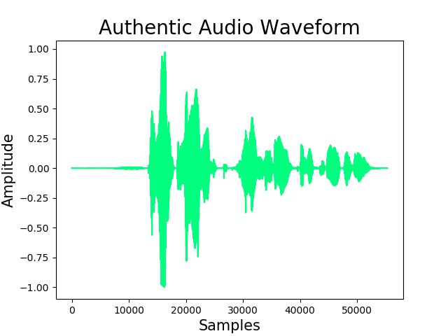
(c)

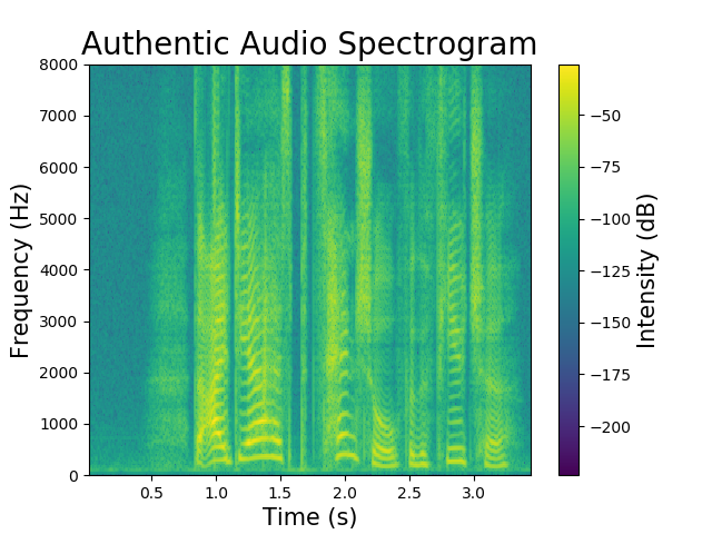
(d)

(e)

(f)

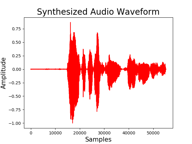
(g)

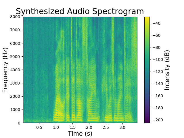
(h)

Figure 3: Audio Waveforms and Spectrograms. Genuine and synthesized audio signals analyzed by the CNN.

Our approach takes advantage of the translation invariant properties of images to find critical, local indicators revealing the authenticity of an audio signal. Furthermore, our approach benefits from shared weights which collectively learn from all patches of a spectrogram. By leveraging signal processing techniques, image processing techniques, and Deep Learning techniques, we detect authentic and inauthentic audio clips with high reliability and accuracy.

III. Problem Formulation

We investigate an audio discrimination task in this paper. Given an audio signal of a few seconds in length, we seek to recognize whether it is genuine human speech or synthesized speech. Our overall approach is shown in Figure 2.

A. Dataset

To validate our methods, we utilize the ASVspoof2019 dataset [27]. This dataset was introduced in the ASVspoof2019: Automatic Speaker Verification Spoofing and Countermeasures Challenge [28]. It contains both genuine human speech samples and fabricated speech samples. The inauthentic speech samples fall into the three categories outlined in Section II-A: voice conversion (VC), speech synthesis (SS), and replay attacks. For this paper, we only consider generated audio. Thus, we only utilize the VC and SS subsets of the dataset. The synthesized audio was generated with neural acoustic models and Deep Learning methods, including LSTMs and Generative Adversarial Networks (GANs). Our final version of the dataset based on only VC and SS attacks contains 121,461 audio tracks. The details of the dataset are included in Table 1. We utilize the official dataset split according to the challenge, which results in 25,380 training tracks, 24,844 validation tracks, and 71,237 testing tracks.

B. Spectrogram Generation

The first step in our analysis is to consider the digital audio signal in the time domain. Let $f(t)$ be the continuous time domain audio signal where $t$ is the time index. $f(t)$ is the original signal provided in the ASVspoof2019 dataset. The average length of all of the audio signals in the entire dataset (including training, validation, and testing samples) is 3.35 seconds. Figure 1 and Figure 3 show examples of time domain audio signals. By a visual inspection, it is unclear which signals could be genuine and which could be synthesized. In order to leverage computer vision techniques for forensic analysis, we convert these time domain signals into frequency domain spectrogram “images”, as shown Figure 3.

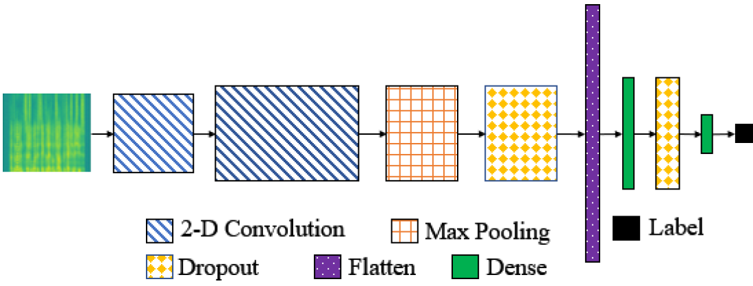
Figure 4: CNN Diagram. The CNN developed for our approach.

Layer	Output Shape (N, H, W)	Parameters
$\text{conv}_{1}$	(32, 48, 32)	320
$\text{conv}_{2}$	(30, 46, 64)	18,496
max pooling	(15, 23, 64)	0
$\text{dropout}_{1}$	(15, 23, 64)	0
$\text{flatten}_{1}$	(22080)	0
$\text{dense}_{1}$	(128)	2,826,368
$\text{dropout}_{2}$	(128)	0
$\text{dense}_{2}$	(2)	258

Table 2: CNN Architecture. This table indicates the parameters of the proposed CNN. Each row in the table specifies (from left to right) the details of the layer, its output shape, and the number of parameters it contains. Output shape is in the form (N, H, W), where N refers to the number of feature maps produced, H refers to the height of the feature maps produced, and W refers to the width of the feature maps produced.

The conversion process involves taking the Discrete Fourier Transform (DFT) of a sampled signal $f[n]$ to obtain Fourier coefficients $F(m)$, where $m$ is the frequency index in hertz (Hz). The magnitudes of the coefficients $|F|$ are then color coded to indicate the strength of the signal. $f[n]$ refers to a sampled, discrete version of $f(t)$ with a total of $N$ samples. The $N$ samples can be denoted as $f[0],f[1],...,f[N-1]$, where each sample $f[n]$ is an impulse with area $f[n]$. The Discrete Fourier Transform is:

$$F(m)=\sum_{n=0}^{N-1}f[n]e^{-\frac{i2\pi}{N}mn}$$ (1)

A Fast Fourier Transform (FFT) is a method that efficiently computes the DFT of a sequence. Therefore, we utilize the FFT to rapidly obtain Fourier coefficients $F(m)$ of the signals in our dataset. For our experiments, we run the FFT on blocks of the signal consisting of 512 sampled points with 511 points of overlap between consecutive blocks. The signals in our dataset have a sample rate of 16 kHz, so the audio signals are sliced into equally-sized temporal segments of 32 milliseconds in length.

Once the Fourier coefficients have been computed, the audio signal $f[n]$ is converted to decibels for magnitude scaling: $f_{dB}=10\log(|f|)$. The spectrogram “image” of size $50\text{x}34$ pixels is then constructed to show the audio signal’s magnitude (i.e., intensity in dB) over time versus frequency, as shown in Figure 3.

Each spectrogram encompasses information from an entire audio track. We can determine frequencies and intensities of an audio signal as it propagates in time by analyzing the colors in the spectrogram from left to right in the image. The warmer and more yellow a color is, the louder the audio signal is at that point in time and at that frequency. Darker colors indicate quieter sounds. Once the spectrogram images are created, they are converted to grayscale images and normalized in preparation for analysis by the CNN.

C. Convolutional Neural Network (CNN)

We employ a Convolutional Neural Network (CNN) to analyze the normalized, grayscale spectrogram images and detect whether they represent genuine or synthesized audio. Table 2 outlines the specifics of the network architecture depicted in Figure 4. It consists mainly of two convolutional layers in the initial stages of the CNN. Then, it employs max pooling and dropout for regularization purposes and to prevent overfitting. The final output of the neural network applies a softmax function to a fully-connected dense layer of two nodes, producing two final detection scores. The scores indicate the probability that the audio segment under analysis is considered to be genuine or synthesized. Finally, the argmax function is used to convert these probabilities into a final class prediction. We train for 10 epochs using the ADAM optimizer [29] and cross entropy loss function.

IV. Experimental Results

Receiver Operating Characteristic Curve                            Precision-Recall Curve

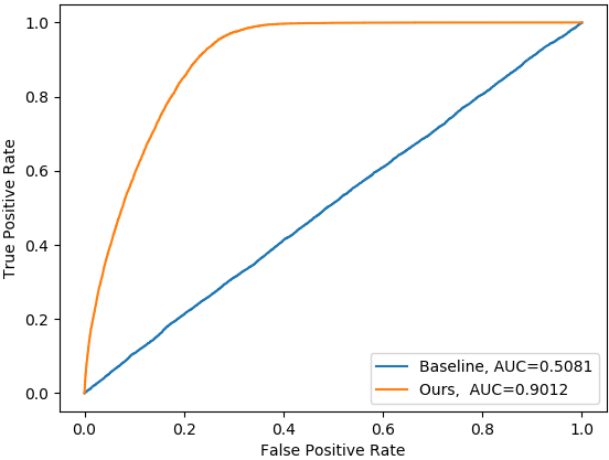
(a)

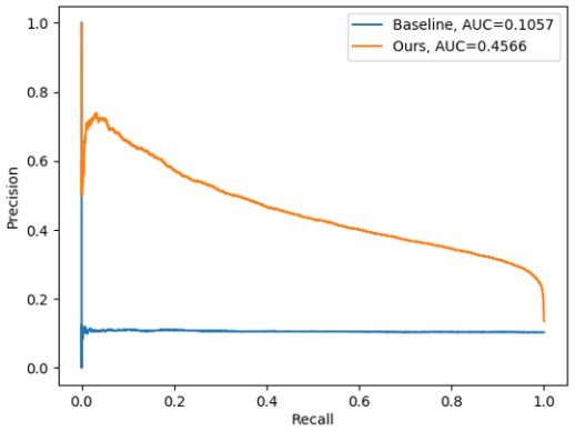
(b)

Figure 5: ROC and PR. Our method is in orange and the baseline random approach is in blue.

Table 3 summarizes the results of our method. For comparison purposes, we evaluate how our approach performs relative to a baseline approach in which the classifier randomly guesses whether an audio signal is genuine or synthesized according to a uniform random distribution. Our spectrogram-CNN achieves 85.99% accuracy on the testing dataset, outperforming the baseline random method by 35.95%. This indicates that our method is considerably better than random chance. The precision, recall, and F1-scores of our method are 67.23%, 75.94%, and 70.08%, respectively. These values further indicate that even on an unbalanced dataset, our method performs well.

Figure 5 shows the Receiver Operating Characteristic (ROC) and Precision-Recall (PR) curves of our method in comparison to the baseline random method. For both of these plots, the ideal, completely accurate classifier would yield curves resembling a 45-degree angle that include the top-left corners of the plots. The closer a curve to that corner, the better a classifier performs. A way to measure the quality of a curve is by calculating the area under the curve (AUC). A higher AUC value indicates a better classifier, with an AUC of 1.0 indicating a “perfect” classifier. Because the ROC and PR metrics do not depend on the class distribution of the dataset, AUC is a useful metric for evaluating classifiers on unbalanced datasets such as ours. Our method yields a high ROC-AUC of 0.9012 and a PR-AUC of 0.4566. In comparison to the baseline method which achieves a ROC-AUC of 0.5081 and a PR-AUC of 0.1057, our method performs better by both metrics.

Considering that the testing dataset contains new audio attacks which were never seen before in training and validation, these results are very promising. They demonstrate that our method generalizes well to some unseen audio attacks. However, there are still some other unseen attacks on which our method fails, and more investigation into its failure cases is needed. In general, though, analysis of audio signals formatted as spectrograms is effective for an audio verification task.

Method	Accuracy	Precision	Recall	F-1
Baseline (Random)	50.06%	49.93%	49.80%	40.63%
Proposed Method	85.99%	67.23%	75.93%	70.08%

Table 3: Results. This table indicates the performances of the baseline random method and our proposed method.

V. Conclusion

In this paper, we propose a CNN approach to analyze audio signal spectrograms for the purpose of validating the audio signal authenticity. The experimental results show that the method accomplishes this discrimination task with high accuracy on the test dataset with a relatively shallow network. Our method generalizes to new audio attacks never seen during training. Thus, our results indicate that a signals-informed and signals-based approach assists a neural network in learning information to extend to new attacks. However, our method fails to classify other new audio signals correctly. Future work should focus on understanding the failure cases and improving our method to correctly identify whether they are fake or real audio signals. A future approach could include analyzing the signals with a Natural Language Processing (NLP) approach to evaluate the coherence of the spoken phrases. Then, two analyses could be conducted in parallel to analyze the frequency content and structure of the signal as well as the coherence of the spoken words. Another future direction could include an environmental analysis of the captured audio signal. If, for example, an audio signal is identified to be recorded outside but the speaker says phrases as if he or she is indoors, this mismatch between recording environment and spoken cues could indicate that the audio is synthesized. These experiments conducted in tandem with our proposed approach would strengthen our audio authentication method.

Author Biography

Emily R. Bartusiak is a Ph.D. student in Electrical and Computer Engineering at Purdue University. She previously earned her B.S. and M.S. in Electrical Engineering from Purdue with a minor in Management. She currently investigates the application of Machine Learning techniques to signals, images, and videos for forensic, defense, and biomedical research.

Edward J. Delp is the Charles William Harrison Distinguished Professor of Electrical and Computer Engineering and Professor of Biomedical Engineering at Purdue University. His research interests include image and video processing, image analysis, computer vision, image and video compression, multimedia security, medical imaging, multimedia systems, communication and information theory.

References

- [1] H. Ajder, G. Patrini, F. Cavalli, and L. Cullen, “The state of deepfakes: Landscape, threats, and impact,” Deeptrace Lab, September 2019.
- [2] R. Toews, “Deepfakes are going to wreck havoc on society. we are not prepared.” Forbes, May 2020.
- [3] Z. Chen, W. Zhang, Z. Xie, X. Xu, and D. Chen, “Recurrent neural networks for automatic replay spoofing attack detection,” Proceedings of the IEEE International Conference on Acoustics, Speech and Signal Processing, April 2018, Calgary, Canada.
- [4] D. Montserrat, H. Hao, S. Yarlagadda, S. Baireddy, R. Shao, J. Horváth, E. R. Bartusiak, J. Yang, D. Güera, F. Zhu, and E. Delp, “Deepfakes detection with automatic face weighting,” Proceedings of the IEEE/CVF Conference on Computer Vision and Pattern Recognition Workshops, June 2020, Seattle, Washington (Virtual).
- [5] A. Rössler, D. Cozzolino, L. Verdoliva, C. Riess, J. Thies, and M. Niessner, “Faceforensics++: Learning to detect manipulated facial images,” Proceedings of the IEEE/CVF International Conference on Computer Vision, August 2019, Seoul, Korea.
- [6] D. Güera and E. Delp, “Deepfake video detection using recurrent neural networks,” Proceedings of the IEEE International Conference on Advanced Video and Signal-based Surveillance, November 2018, Auckland, New Zealand.
- [7] E. R. Bartusiak, S. K. Yarlagadda, D. Güera, P. Bestagini, S. Tubaro, F. M. Zhu, and E. J. Delp, “Splicing detection and localization in satellite imagery using conditional gans,” Proceedings of the IEEE Conference on Multimedia Information Processing and Retrieval, March 2019, San Jose, CA.
- [8] D. Güera, S. Baireddy, P. Bestagini, S. Tubaro, and E. Delp, “We need no pixels: Video manipulation detection using stream descriptors,” Proceedings of the International Conference on Machine Learning, Synthetic-Realities: Deep Learning for Detecting AudioVisual Fakes Workshop, June 2019, Long Beach, CA.
- [9] A. Chintha, B. Thai, S. J. Sohrawardi, K. M. Bhatt, A. Hickerson, M. Wright, and R. Ptucha, “Recurrent convolutional structures for audio spoof and video deepfake detection,” IEEE Journal of Selected Topics in Signal Processing, June 2020.
- [10] B. Bogert, M. Healy, and J. Tukey, “The quefrency alanysis of time series for echoes: Cepstrum, pseudo autocovariance, cross-cepstrum and saphe cracking,” Proceedings of the Symposium on Time Series Analysis, vol. 15, pp. 209–243, June 1963, New York, NY.
- [11] S. Stevens, J. Volkmann, and E. Newman, “A scale for the measurement of the psychological magnitude pitch,” Journal of the Acoustical Society of America, vol. 8, pp. 185–190, June 1937.
- [12] D. Purves and G. Fitzpatrick, “Neuroscience,” The Audible Spectrum, vol. 2nd Edition, 2001, Sunderland, MA.
- [13] N. Ahmed, T. Natarajan, and K. Rao, “Discrete cosine transform,” IEEE Transactions on Computers, vol. 23, pp. 90–93, January 1974.
- [14] M. Sahidullah and G. Saha, “Design, analysis, and experimental evaluation of block based transformation in mfcc computation for speaker recognition,” Speech Communication, vol. 54, pp. 543–565, May 2012.
- [15] Z. Chen, Z. Xie, W. Zhang, and X. Xu, “Resnet and model fusion for automatic spoofing detection,” Proceedings of the Conference of the International Speech Communication Association, August 2017.
- [16] P. Verma and J. Smith, “Neural style transfer for audio spectrograms,” Proceedings of the Conference on Neural Information Processing Systems, Workshop for Machine Learning for Creativity and Design, December 2017, Long Beach, CA.
- [17] J. Dennis, H. D. Tran, and H. Li, “Spectrogram image feature for sound event classification in mismatched conditions,” IEEE Signal Processing Letters, vol. 18, no. 2, pp. 130–133, 2011.
- [18] Yih Nen Jeng and You-Chi Cheng, “A first study of speech processing via a novel mode decomposition based on the fourier sine spectrum and spectrogram,” Proceedings of the IEEE Region 10 Conference, October 2007, Taipei, Taiwan.
- [19] S. Greenberg and B. E. D. Kingsbury, “The modulation spectrogram: in pursuit of an invariant representation of speech,” Proceedings of the IEEE International Conference on Acoustics, Speech, and Signal Processing, April 1997, Munich, Germany.
- [20] M. Stolar, M. Lech, R. S. Bolia, and M. Skinner, “Acoustic characteristics of emotional speech using spectrogram image classification,” Proceedings the IEEE International Conference on Signal Processing and Communication Systems, December 2018, Cairns, Australia.
- [21] L. Zheng, Q. Li, H. Ban, and S. Liu, “Speech emotion recognition based on convolution neural network combined with random forest,” Proceedings of the Chinese Control And Decision Conference, June 2018, Shenyang, China.
- [22] S. Prasomphan, “Detecting human emotion via speech recognition by using speech spectrogram,” Proceedings of the IEEE International Conference on Data Science and Advanced Analytics, October 2015, Paris, France.
- [23] S. Prasomphan, “Improvement of speech emotion recognition with neural network classifier by using speech spectrogram,” Proceedings of the International Conference on Systems, Signals and Image Processing, September 2015, London, UK.
- [24] T. Mittal, U. Bhattacharya, R. Chandra, A. Bera, and D. Manocha, “Emotions don’t lie: A deepfake detection method using audio-visual affective cues,” arXiv, March 2020.
- [25] H. Malik, “Securing voice-driven interfaces against fake (cloned) audio attacks,” Proceedings of the IEEE Conference on Multimedia Information Processing and Retrieval, March 2019, San Jose, CA.
- [26] L. He, M. Lech, N. C. Maddage, and N. Allen, “Stress detection using speech spectrograms and sigma-pi neuron units,” Proceedings of the IEEE International Conference on Natural Computation, August 2009, Tianjin, China.
- [27] J. Yamagishi, M. Todisco, M. Sahidullah, H. Delgado, X. Wang, N. Evans, T. Kinnunen, K. Lee, V. Vestman, and A. Nautsch, “Asvspoof 2019: The 3rd automatic speaker verification spoofing and countermeasures challenge database,” University of Edinburgh. The Centre for Speech Technology Research, 2019.
- [28] M. Todisco, J. Yamagishi, M. Sahidullah, H. Delgado, X. Wang, N. Evans, T. Kinnunen, K. Lee, V. Vestman, and A. Nautsch, “Asvspoof 2019: Automatic speaker verification spoofing and countermeasures challenge evaluation plan,” ASVspoof Consortium, January 2019.
- [29] D. Kingma and J. Ba, “Adam: A method for stochastic optimization,” Proceedings of the International Conference for Learning Representations, May 2015, San Diego, CA.