TartanDrive: A Large-Scale Dataset for Learning
Off-Road Dynamics Models

Abstract

We present TartanDrive, a large scale dataset for learning dynamics models for off-road driving. We collected a dataset of roughly 200,000 off-road driving interactions on a modified Yamaha Viking ATV with seven unique sensing modalities in diverse terrains. To the authors’ knowledge, this is the largest real-world multi-modal off-road driving dataset, both in terms of number of interactions and sensing modalities. We also benchmark several state-of-the-art methods for model-based reinforcement learning from high-dimensional observations on this dataset. We find that extending these models to multi-modality leads to significant performance on off-road dynamics prediction, especially in more challenging terrains. We also identify some shortcomings with current neural network architectures for the off-road driving task. Our dataset is available at https://github.com/castacks/tartan_drive.

I Introduction

Robots need to understand the physical properties of the world to deal with its complexity in practical tasks such as off-road driving. Robots should not only rely on the geometric and semantic information of observed scenes, but also reason about dynamical features, such as the vehicle speed and approach angle, to avoid getting stuck or damaged in various types of terrain, such as puddles, tall grass, and loose gravel.

Modeling this complex interplay between the robot and the environment is extremely difficult using traditional methods, which typically rely on high-fidelity models of both the dynamics of the robot, as well as the environment that it interacts with [1]. Data-driven methods [2, 3, 4] have been explored to address this issue and have shown great potential, but still require large-scale diverse datasets for the training.

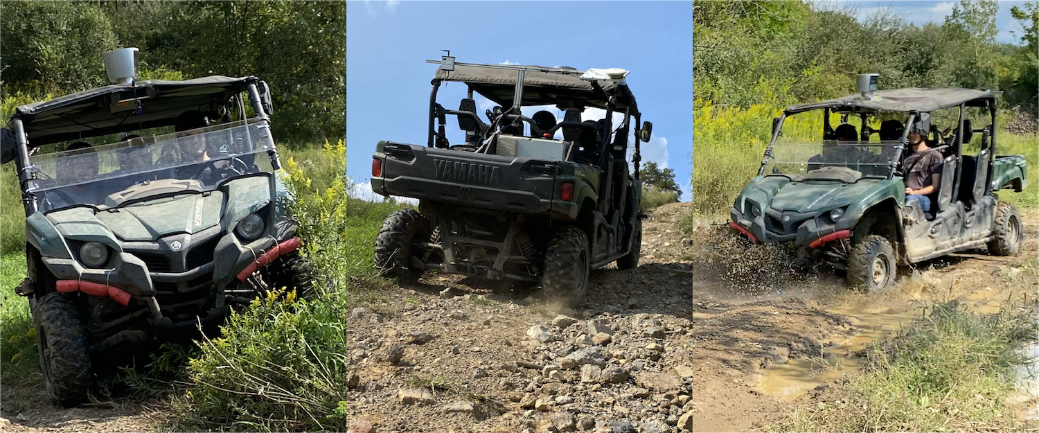
Figure 1: We provide a rich dataset for learning off-road vehicle dynamics. Data was collected by driving a modified ATV through a variety of terrain including tall grass, rocks, and mud. Driving data consists of robot actions, and a variety of multi-modal observations.

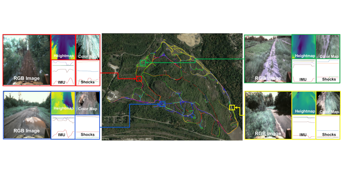
Figure 2: Our dataset contains several hours of driving data from a test site in Pittsburgh, PA. Our dataset contains diverse off-road driving scenarios and several sensing modalities, including front-facing camera and top-down local maps. Shown in the center is a satellite image of the testing site with trajectories superimposed. They are colored according to a clustering based on ResNet [5] features on the RGB images. Shown on the sides are four datapoints (one from each cluster) with five of the seven modalities available in the dataset shown. We can observe a diverse set of scenarios, including dense foliage (red), steep slopes (green) open road (blue) and puddles (yellow).

While many autonomous driving datasets exist, most focus on urban environments [6, 7, 8, 9, 10]. For off-road driving, existing datasets only focus on scene understanding, with a special focus on semantic segmentation [11, 12, 13, 14, 15, 16]. We argue the semantic labels (i.e. dirt, grass, tree, bush, mud) are not sufficient. For example, a bush might be traversable for one robot but not for another less capable robot. Additionally, a robot could get stuck in mud at low speed but not at high speed. This information is hard to obtain from camera and LiDAR sensors alone. Rather, it is more feasible to learn these properties from interaction data, which can include data from robot actions, wheel encoders and IMU.

There is also an increasing interest in developing datasets for understanding physical common-sense and predicting interactions between objects. However, they either utilize a simulated world with simple objects such as a pile of blocks [17, 18, 19] or are collected in controlled laboratory environments [20, 21, 22].

We present a large and diverse real-world off-road driving dataset, which contains multi-modal interaction data in various complex terrains, including challenging interactions such as driving through dense vegetation and puddles, driving on steep slopes, and driving at high speed with tire slip. We believe this dataset will not only benefit the development of autonomous off-road driving, but also facilitate research in modeling complex robot dynamics.

This dataset is motivated by two points. First, accurately modeling off-road vehicle dynamics is difficult, especially in real-world scenarios. While some approaches leverage analytical models of the terrain [1], these models are often low fidelity since it is intractable to correctly model complex interactions such as collisions with rocks and gravel, tire interactions with arbitrary surfaces, etc. Recent work [2, 3] leverages off-road driving datasets to create data-driven dynamics models instead. However, existing datasets are limited in either the amount or diversity of data, or the amount of modalities available. Second, data-driven models can benefit from supervision from multi-modal sensory input. Tremblay et al. [3, 23] have shown that leveraging various sensing modalities leads to learned models that are more robust to challenging and inconstant dynamics.

The contributions of this work are as follows:

1. A large-scale dataset collected on a Yamaha ATV in off-road scenarios, containing roughly 200,000 interaction datapoints with multiple high-dimensional sensing modalities. To the best of the authors’ knowledge, this exceeds the largest multi-modal interaction dataset for off-road driving [23] in both the number of available datapoints and modalities.

2. Benchmarks of several state-of-the-art neural network architectures and training procedures [24, 25, 26] for high-dimensional observations in a real-world scenario with challenging dynamics.

II Related Work

Most publicly-available off-road driving datasets focus on understanding environmental features instead of the interplay between the robot and the environment [27]. RUGD [12] consists of video sequences with segmentation label of 24 unique category annotations. Maturana et al. [11] collected a segmentation dataset, which tried to explore more fine-grained information such as traversable grass and non-traversable vegetation, but those discrete labels are still too abstract to understand how a robot is going to behave in the specific case. Gresenz et al. [28] collected a dataset containing over 10000 images of offroad bicycle driving and labels corresponding to the roughness of the terrain in the image, where the labels were generated from processing sensory data available on the platform. Similarly, this dataset does not provide enough interaction data or actions. Rellis 3D [15] consists of images, pointclouds, robot states, and actions, but the amount of trajectory data is rather small (about 20 minutes – 12,000 datapoints at 10hz – total). Generally, learning dynamics models requires on the order of hundreds of thousands of dynamics interactions. As our dataset is designed to focus on dynamics models with multi-modal sensory inputs without the need for hand-labeling, we are able to collect much more data than existing datasets.

More and more off-road driving research has taken account of the robot-environment interaction rather than environment features alone to improve the driving performance. Due to the lack of publicly-available real-world datasets, they usually train their models in simulation environments or collect their own data in a small scale or for a specific research purpose. Tremblay et al. [3] trained a multi-modal dynamics model in a simulation environment based on Unreal Engine, and a small forest dataset (Montmorency) [23]. Sivaprakasam et al. [29] developed a simulation environment with random obstacles to learn a predictive model from physical interaction data. Similarly, Wang et al. [4] trained a probabilistic dynamics model for planning using a simulator and a small robot platform. Kahn et al. [2] employ a model-based RL technique in order to enable a wheeled robot to navigate off-road terrain using a monocular front-facing camera [2]. Their algorithm (BADGR) leverages many hours of trajectory data collected via random exploration in order to train a neural network to model the dynamics of the robot over various types of terrain. In addition to using the position of the robot, the authors also utilize hand-designed events calculated from the on-board IMU and LiDAR as additional supervision for the model. The authors make their data publicly-available, where the data consists of the hand-designed events (such as bumpiness and collision), RGB images, robot states, and actions.

On the other hand, learning a dynamics model has been an active research area in various directions such as model-based reinforcement learning (RL). Most work in RL literature learns the model in simulation environments. For the off-road driving task, [2] learned from the interaction data a classification network to predict the hand-designed events (i.e. collision, smoothness, etc.). Tremblay et al. [3] modify the recurrent state-space model of Hafner et al. [25] to handle multiple modalities and provide a modified training objective. Wang et al. [4] improve trajectory prediction by incorporating uncertainty estimation and a closed-loop tracker. In this paper, we follow these papers and test several neural network architectures to demonstrate the potential value of the proposed TartanDrive dataset.

Dataset	Samples	State	Action	Image	Pointcloud	Heightmap	RGBmap	IMU	Wheel RPM	Shocks	Intervention
RUGD	2700	No	No	Yes	No	No	No	No	No	No	No
Rellis 3D	13800	Yes	Yes	Yes	Yes	No	No	Yes	No	No	No
Montmorency	75000	Yes	Yes	Yes	Yes	Yes	No	Yes	No	No	No
Ours	184000	Yes	Yes	Yes	No	Yes	Yes	Yes	Yes	Yes	Yes

TABLE I: Overview and comparison of various off-road driving datasets

III The Dataset

Our off-road driving dataset is designed for the purpose of dynamics prediction. As such, it contains a large number of interaction data over a diverse set of terrains and scenarios.

Modality	Type	Dimension	Train Dimension
Robot Pose	Vector	7	7
RGB Image	Image	2 x 1024 x 512	128 x 128
Heightmap	Image	500 x 500	64 x 64
RGB Map	Image	500 x 500	64 x 64
IMU	Time-series	20 x 6	20 x 6
Shock Position	Time-series	5 x 4	20 x 4
Wheel RPM	Time-series	5 x 4	20 x 4
Intervention	Boolean	1	1

TABLE II: The set of available dataset features and their sizes.

III-A ATV Platform

We use a Yamaha Viking All-Terrain Vehicle (ATV) which was previously modified by Mai et al. [30] to collect data. The throttle and steering of the ATV were controlled using a Kairos Autonomi steering ring and servos via a joystick. For safety reasons, the brakes were controlled directly by a human driver.

Proprioceptive and exteroceptive sensors were used to collect real time data. First, a forward facing Carnegie Robotics Multisense S21 stereo camera provided long range, high resolution stereo RGB and depth images, as well as inertial measurements. A NovAtel PROPAK-V3-RT2i GNSS unit provided global pose estimates. A Racepak G2X Pro Data Logger recorded suspension shock travel and wheel rpm at all four wheels, as well as the position of the brake pedal. All sensors and servos were connected to an on-board computer running ROS. Joystick control inputs were relayed to the servos. Figure 3 shows a system diagram.

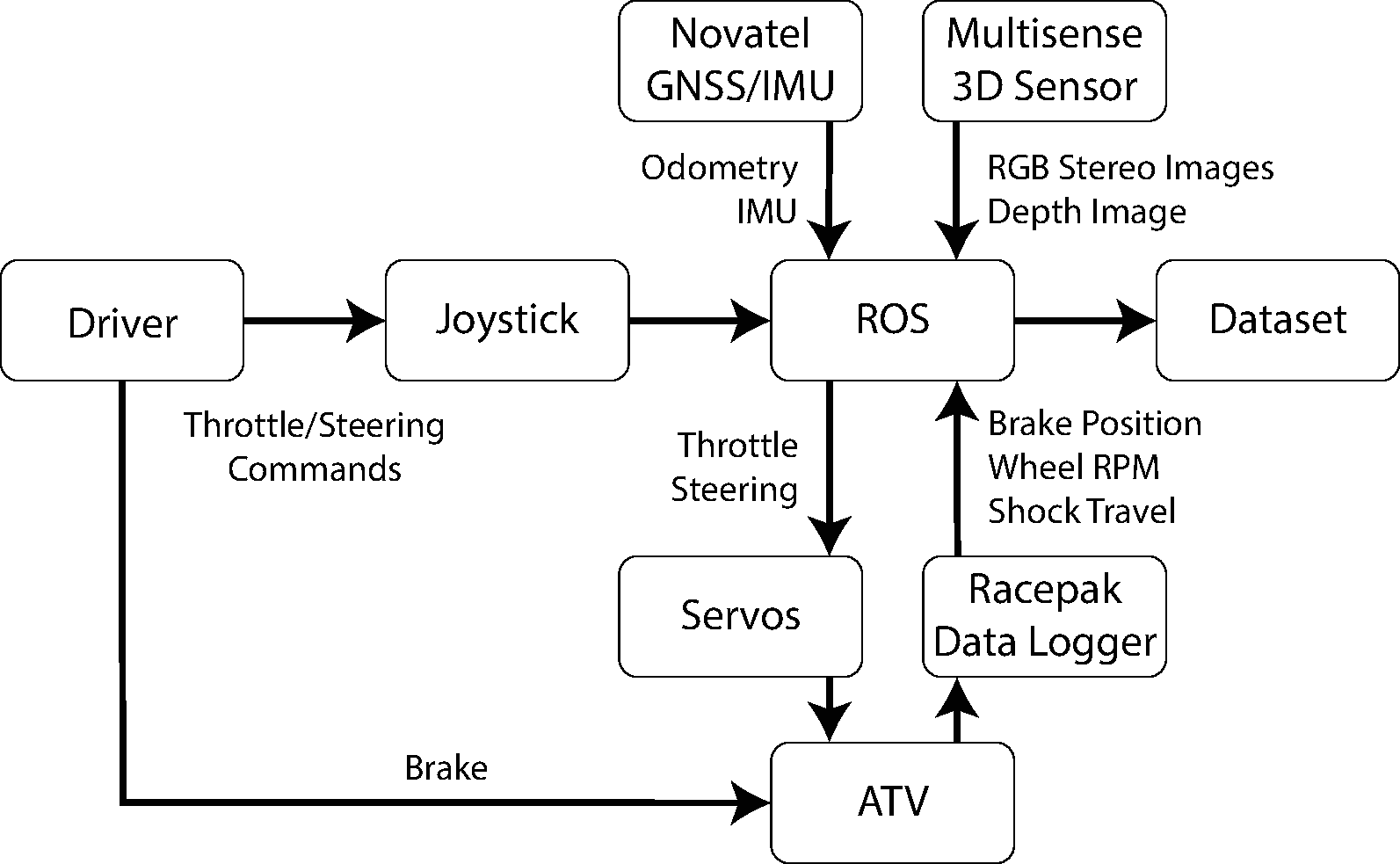
Figure 3: A system diagram of our data collection setup. We use multiple sensors to collect interaction data across many modalities, as well as throttle and steering commands.

III-B Data Collection

We collected data in a diverse range of terrains, including rocks, mud, foliage, as shown in Figure 1. During data collection, we opted to use human tele-operated controls instead of random controls since it may have resulted in catastrophic injuries to the vehicle or on-board passengers. In total, we collected 630 trajectories equivalent to five hours of data. Each trajectory was kept short and ended whenever the driver intervened by applying the brakes.

Data were collected at 10Hz, and consisted of raw sensor data as well as post-processed data. Each observation modality is described below with a summary in Table II. Note that we upsample the 50Hz wheel proprioception to 200Hz to match the frequency of the IMU.

III-B1 Robot Action

Actions $a=(\mu_{t},\mu_{s})$ were two-dimensional and corresponded to desired throttle and steering positions. Throttle commands took values between 0 and 1, with 1 corresponding to wide open throttle. Steering commands took values between -1 and 1, with -1 corresponding to a hard left turn. The commands were executed by the servos using PID position control.

III-B2 Robot Pose

Robot poses were estimated from the NovAtel GNSS unit. They took the form of a concatenated position vector $p=(x,y,z)$ and quaternion orientation $q=(q_{x},q_{y},q_{z},q_{w})$.

III-B3 Images

At each timestep, two RGB images were recorded from the onboard stereo camera.

III-B4 Local Terrain Maps

We generate a local top-down-view height map $M_{h}\in\mathbb{R}^{(w\times h\times 2)}$ (two channels to represent the minimum height and maximum height) and a local RGB map $M_{c}\in\mathbb{N}^{(w\times h\times 3)}$ using the stereo images from the Multisense S21 sensor. As shown in Fig. 5, we first generate a disparity image using a stereo matching network [31], and estimate the camera motion using TartanVO network [32]. Given the camera intrinsics and the corresponding RGB image, we register and colorize each pointcloud into the camera’s current frame. Then the registered local 3D point cloud is projected to the ground plane, and then binned, producing a top-down map. We used a resolution of $0.02$ m/pixel, and a region of $(0,10)$ m in the forward direction, $(-5,5)$ m in the lateral direction, which result in a map size of $500\times 500$. The maps are updated at 10 Hz.

III-B5 Proprioceptive Data

We recorded inertial data (angular velocity and linear acceleration) from the Multisense sensor, as well as shock travel and wheel rpm from the Racepak data logger. Since these sensors made measurements faster than 10Hz, we recorded multiple measurements at each time step in the form of time-series data. The inertial data had a time-series length of 20. The shock travel and wheel rpm data had a time-series length of 5.

III-B6 Intervention Data

Due to safety concerns, the driver was allowed to stop the ATV using the brake pedal. We recorded the brake pedal position, and a boolean intervention signal that indicated when the brakes exceeded a threshold.

III-C Dynamical Variation in the Dataset

How the robot moves depends on the physical properties of the robot, the action command we send, and the physical properties of the environment. In simple environments such as urban roads, the robot properties and actions are sufficient to perform accurate trajectory prediction. We thus ask the question: does our dataset capture the dynamical variation induced by different types of terrains? To answer this question, we first perform a motivational experiment to quantify the correlation between future states and action sequences. The rationale behind this experiment is that if significant dynamical variations exist due to different terrains, then we would expect that similar sequences of actions in the dataset may yield very different trajectories.

In order to perform this experiment, we first collected 10000 random subsequences of length 10 (one second) from our dataset and computed the displacement and rotation from the initial state to the final state (such that every trajectory began from the same initial state). We then performed time-series clustering (using [33]) on the corresponding sequences of actions. One important note is that we chose simple Euclidean distance instead of time-warping methods [34] as both the duration and temporal position of the actions in the sequence (and not just the shape of the sequence) affect state displacement. We then computed a t-Distributed Stochastic Neighbor Embedding (t-SNE) [35] of the state displacements and colored each embedded point according to its corresponding action cluster. To mitigate the effect of velocity on the final state displacement, we binned our data based on initial speed and created a separate visualization for each bin. One of the resulting visualizations is shown in Figure 4. The remainder of the figures, a more detailed desription of the clustering process and the experiment hyperparameters are in the Appendix .

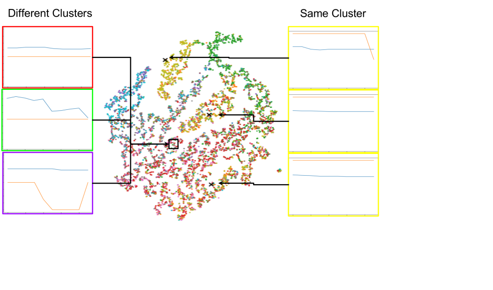
Figure 4: One t-SNE embedding of the state displacements in the dataset. Each point is colored according to its closest action sequence centroid. We can observe from this figure that there is some correlation between the clusters and their position in the t-SNE embedding, though the colors clearly mix. Shown on the left are three action sequences from different clusters that map to the same region in the embedding space. Conversely, shown on the right are three action sequences that map to very different regions of the embedding space, despite being very similar.

As we can observe in Figure 4, there is indeed some clustering of state displacements, but many clusters blend together in the visualization. Additionally, the same action cluster does not necessarily form a single cluster in the t-SNE visualization, nor does a single cluster in the t-SNE visualization consist of points belonging to the same action cluster. This confirms our hypothesis that while there is (obviously) a correlation between actions and state displacements, correct dynamics prediction in our dataset requires more features than just the action sequence.

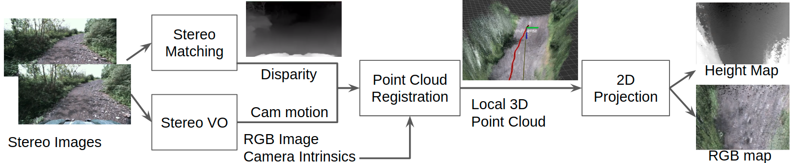
Figure 5: A diagram of the mapping pipeline. We use the stereo images from the Multisense S21 sensor to generate a top-down height map and a top-down RGB map.

IV Multi-modal Modeling

In addition to data collection, we benchmarked several recent neural network architectures for dynamics prediction from high-dimensional data. For this work, we consider the task of dynamics prediction to be the prediction of future states $s_{1:T}$, given an intital state $s_{0}$, a sequence of actions $a_{1:T}$, and a set of observations $O_{0}=\{o^{m}_{0}\}$ from a set of modalities $M$. These models thus take the form $f_{\theta}(s_{0},a_{1:T},O_{0})$.

IV-A Multi-modal Modeling on the ATV

We first describe the general architecture of our latent-space model for off-road dynamics prediction. Similar to prior work [24, 3], we use a latent-space model that is comprised of three parts:

1. An encoder $e_{\theta}(o_{t}):\mathcal{O}\rightarrow\mathcal{Z}$ that maps a high-dimensional observation $o_{t}$ into the latent space

2. A model $f_{\theta}(z_{t},a_{t}):(\mathcal{Z},\mathcal{A})\rightarrow\mathcal{Z}$ that forward-simulates the model in latent space, given actions.

3. A decoder $d_{\theta}(z_{t}):\mathcal{Z}\rightarrow\mathcal{O}$ that maps the low-dimensional latent state back to the observation space.

Parameterizing the model in this fashion allows for efficient state prediction, as one only needs to encode the initial observation $o_{0}$ to get an initial latent state $z_{0}$. From this, state vectors $s_{1:T}$ can be recovered via forward-simulating the latent model to get $z_{1:T}$ and then decoding state without decoding the high-dimensional observations. A detailed description of the network architecture is provided in the Appendix. We now describe the specific implementation of our model for the ATV.

Multi-modal Encoders

The encoder for our model consists of a deep neural network for each modality $m$. The original size, and rescaled training size of each modality used is shown in Table II. The neural network architectures used for the different modality types are as follows:

1. Vector inputs were passed through a dense network to produce a Gaussian distribution $p(z)$.

2. Images were passed through a convolutional neural network (CNN), flattened, and passed through a dense network to produce $p(z)$.

3. Time-series inputs were passed through a WaveNet encoder [36], flattened, and passed through a dense network.

To combine the multiple predictions on $p(z)$, we follow previous work [37, 3] which use a product of experts [38]. In this formulation, the aggregated probability of the latent state, $p(z)$, is determined by the product of probabilities of each expert $\prod_{i}q_{i}(z|o_{i})$. This formulation is preferable over a mixture of experts for its ability to produce sharper distributions and allow experts to focus on smaller regions of the prediction space. Since our encoders output diagonal Gaussian distributions in $\mathcal{Z}$, use the result from Cao et al. [39],

$$\begin{split}p(z|\textbf{O})=\prod_{i}q_{i}(z|o_{i})=\mathcal{N}\left(\frac{\sum_{i}(\frac{\mu_{i}}{\sigma_{i}})}{\sum_{i}\frac{1}{\sigma_{i}}},\mathbb{I}\left(\sum_{i}\frac{1}{\sigma_{i}}\right)\right)\end{split}$$ (1)

Latent Model

Our latent model is implemented as a Gated Recurrent Unit (GRU) [40]. While prior work [24, 3] use the Recurrent State-Space model, we found that its performance was similar to a GRU for our particular task.

Decoders

We used several different decoder architectures to address the multi-modality of our observations.

1. Vector outputs were handled using a dense network.

2. Image outputs were handled by using deconvolutional layers to upsample $z$.

3. Time-series outputs were handled by using temporal deconvolutional layers to upsample $z$.

IV-B Training The Latent Space Model

We experimented with three different variations of training loss for our experiments.

IV-B1 State Reconstruction

This loss trained the model to maximize log-probability of ground-truth states (position and orientation) from the Novatel, given the initial states, initial observations and sequences of actions. Note that this loss does not train observation decoders.

$$\mathcal{L}_{state}=-logp_{\theta}(s_{1:T}|o_{0},s_{0},a_{1:T})$$ (2)

IV-B2 Reconstruction Loss

This loss maximizes the log-probability of all observations in addition to the state.

$$\mathcal{L}_{rec}=\mathcal{L}_{state}-\sum_{m}[\beta_{m}logp_{\theta}(o^{m}_{1:T}|z_{1:T})]$$ (3)

Note that $\beta_{m}$ allows us to re-weight the importance of each modality.

IV-B3 Contrastive Loss

Hafner et al. [24] observed that Bayes’ rule can be applied to the reconstruction terms to derive a contrastive loss. Since the contrastive loss is expressed using the latent code $z$, a potential benefit is the ability to ignore distractors in the observation space that are irrelevant to dynamics prediction, e.g. image backgrounds. The contrastive loss is defined as:

$$\mathcal{L}_{con}= \mathcal{L}_{state}-$$ (4)

$$\beta\bigg{[}logp_{\theta}(z_{1:T}|O_{1:T})-\sum_{O^{\prime}_{1:T}}logp_{\theta}(z_{1:T}|O^{\prime}_{1:T})\bigg{]},$$

where the added objective aims to maximize the log-probability of the latent code $z$ given the corresponding observation $O$, while minimizing the log-probability of $z$ given the other observations in the batch $O^{\prime}$. Note that while the terms of the reconstruction loss can be decomposed into independent probabilities, the contrastive loss cannot. As such, there is a single weighting constant $\beta$.

V Experiments and Analysis

Our experiments aim to answer the following questions:

1. Does varying the loss type improve model accuracy?

2. Does using multi-modal sensory data lead to improved dynamics prediction in challenging environments?

V-A Does the Loss Type Matter?

We find that all three loss functions led to similar model accuracy. We attribute this to the fact that in many cases, the high-dimensional sensory inputs are not necessarily correlated with robot motions as they are in the environments used by Hafner et al. [24]. In these simulated environments, predicting future observations is always possible since environments consist only of the agent and a static background. However, future observations are much more difficult to predict in our scenarios. For example, if the ATV drives around a corner, it will be unable to predict observations without some form of mapping and prior traversal. As such, we observe that the auxiliary task of predicting sensory input yields little performance increase.

V-B Does Adding Additional Modalities Help?

We divided our dataset into a set of training trajectories and evaluation trajectories. We then trained four latent-space models with the following varied input modalities:

1. RGB image only, as in [2] (Image)

2. RGB image, heightmap and RGB map (Image + Maps)

3. IMU, shock position and wheel RPM (Time-series)

4. All Modalities (All)

We trained each model using each loss function described in the previous section. We also implemented a baseline kinematic bicycle model (KBM) that leveraged the average wheel RPM to make predictions. Table III shows the accuracy of each model as the root mean squared error (RMSE) of the mean state prediction after 20 steps of forward-simulation. The model with the lowest score for a given loss (i.e. the best set of modalities) is bolded. The model with the lowest evaluation score for a given modality (i.e. the best loss function) is colored in red. Note that since the KBM is not a latent-space model, we copy its evaluation score across all loss columns.

	State	Reconstruction	Contrastive
KBM	1.1638	1.1638	1.1638
Image	0.5263	0.4740	0.4952
Image + Maps	0.3521	0.3386	0.3741
Time Series	0.2176	0.2285	0.1966
All	0.1896	0.1674	0.1958

TABLE III: Model prediction results showing RMSE of mean state prediction for different models and loss functions.

Overall, we can observe that adding additional modalities to the latent-space model results in improved prediction accuracy. The most noticeable improvement comes from adding top-down maps to the image-only model, yielding a 33% decrease in prediction error. From our results, we can gather that the time-series data is very important to the overall dynamics prediction. This is evidenced by the large increase in model accuracy from adding the time-series data (roughly 45% improvement from Image + Maps to All across all training procedures), and the relatively high accuracy of the time-series model. This is to be expected, as wheel RPM in particular is highly correlated with the velocity. However, we still observe that adding the image-based modalities to the time-series model yielded roughly a 15% increase in model accuracy across all training procedures. We note that the performance of the time-series and all-modality models are essentially the same under the contrastive loss.

We also ran experiments to characterize the impact of exteroceptive sensing on out learned models in more challenging driving scenarios. In order to quantify this effect, we compared the prediction accuracy of time-series input only models to prediction accuracy of models incorporating exteroception from the maps and images in both the original dataset, and a new dataset separately collected exclusively in more uneven terrain. We define a trajectory difficulty metric as average change in height per second, which roughly corresponds to terrain steepness and unevenness. The original and new dataset had median trajectory difficulties of $0.0866m/s$ and $0.2253m/s$, respectively. 87% of the trajectories in the new dataset were more difficult than the median difficulty in the original dataset. Table IV shows the prediction accuracy of time-series and all-modality models on each evaluation set, as well as the percent improvement.

Dataset	Prop. Error	Prop. + Ext. Error	Improvement
Original	0.2176	0.1896	13%
Difficult	0.7313	0.5394	26%

TABLE IV: Comparison of Proprioception-only (Prop.) and Proptioception + Exteroception (Prop. + Ext.) Models on the Original and More Difficult Evaluation Datasets

Overall, we observe that the additional vision-based modalities are more beneficial in the more challenging scenarios. This makes sense, as the difficulty of the terrain increases, it becomes increasingly difficult to accurately predict the future using proprioception alone.

VI Conclusions and Future Work

We have presented TartanDrive, a large-scale dataset for training of deep neural networks for dynamics prediction using multiple sensing modalities. We have also provided a benchmark of recent neural network architectures for dynamics prediction from high-dimensional inputs. We plan to continue collecting data and make the dataset potentially useful for tasks other than dynamics prediction, for instance imitation learning.

An obvious direction for future work is the incorporation of these models into a navigation stack. While we have demonstrated acceptable dynamics prediction, it remains to be seen whether this improved dynamics prediction is sufficient for intelligent navigation over rough terrain. We believe that additional research will be necessary to create effective cost functions and planning algorithms that can also leverage the corpus of data we have collected for this work.

Another interesting direction for future work would be the combination of deep latent models and mapping-based approaches. As mentioned in the analysis section, the added partial observability of real-world navigation compared to simulation tasks renders auxiliary sensory prediction tasks largely unhelpful. Additionally, the latent models are not trained on sequences long enough to facilitate learning some form of SLAM. We believe that incorporating some sort of mapping-based approach could allow deep models to exhibit more long-term reasoning capabilities by storing past observations (and potentially features, like in Tung et al. [41]) on a map.

References

- [1] T. M. Howard and A. Kelly, “Optimal rough terrain trajectory generation for wheeled mobile robots,” The International Journal of Robotics Research, vol. 26, no. 2, pp. 141–166, 2007.
- [2] G. Kahn, P. Abbeel, and S. Levine, “Badgr: An autonomous self-supervised learning-based navigation system,” IEEE Robotics and Automation Letters, vol. 6, no. 2, pp. 1312–1319, 2021.
- [3] J.-F. Tremblay, T. Manderson, A. Noca et al., “Multimodal dynamics modeling for off-road autonomous vehicles,” IEEE International Conference on Robotics and Automation, 2020.
- [4] S. J. Wang, S. Triest, W. Wang et al., “Rough terrain navigation using divergence constrained model based reinforcement learning,” in Conference on Robot Learning. PMLR, 2021.
- [5] K. He, X. Zhang, S. Ren, and J. Sun, “Identity mappings in deep residual networks,” in European conference on computer vision. Springer, 2016, pp. 630–645.
- [6] J. Geyer, Y. Kassahun, M. Mahmudi et al., “A2D2: Audi Autonomous Driving Dataset,” 2020. [Online]. Available: https://www.a2d2.audi
- [7] “Waymo open dataset: An autonomous driving dataset,” 2019.
- [8] M.-F. Chang, J. W. Lambert, P. Sangkloy et al., “Argoverse: 3d tracking and forecasting with rich maps,” in Conference on Computer Vision and Pattern Recognition, 2019.
- [9] M. Cordts, M. Omran, S. Ramos et al., “The cityscapes dataset for semantic urban scene understanding,” in Proc. of the IEEE Conference on Computer Vision and Pattern Recognition, 2016.
- [10] W. Maddern, G. Pascoe, C. Linegar, and P. Newman, “1 Year, 1000km: The Oxford RobotCar Dataset,” The International Journal of Robotics Research, vol. 36, no. 1, pp. 3–15, 2017. [Online]. Available: http://dx.doi.org/10.1177/0278364916679498
- [11] D. Maturana, P.-W. Chou, M. Uenoyama, and S. Scherer, “Real-time semantic mapping for autonomous off-road navigation,” in Field and Service Robotics. Springer, 2018, pp. 335–350.
- [12] M. Wigness, S. Eum, J. G. Rogers et al., “A rugd dataset for autonomous navigation and visual perception in unstructured outdoor environments,” in International Conference on Intelligent Robots and Systems, 2019.
- [13] A. Valada, G. L. Oliveira, T. Brox, and W. Burgard, “Deep multispectral semantic scene understanding of forested environments using multimodal fusion,” in International symposium on experimental robotics. Springer, 2016, pp. 465–477.
- [14] L. Dabbiru, C. Goodin, N. Scherrer, and D. Carruth, “Lidar data segmentation in off-road environment using convolutional neural networks (cnn),” SAE International Journal of Advances and Current Practices in Mobility, vol. 2, no. 2020-01-0696, pp. 3288–3292, 2020.
- [15] P. Jiang, P. Osteen, M. Wigness, and S. Saripalli, “Rellis-3d dataset: Data, benchmarks and analysis,” 2020.
- [16] A. Shaban, X. Meng, J. Lee et al., “Semantic terrain classification for off-road autonomous driving,” in Conference on Robot Learning. PMLR, 2022, pp. 619–629.
- [17] P. W. Battaglia, R. Pascanu, M. Lai et al., “Interaction networks for learning about objects, relations and physics,” in NIPS, 2016.
- [18] A. Lerer, S. Gross, and R. Fergus, “Learning physical intuition of block towers by example,” in International conference on machine learning. PMLR, 2016, pp. 430–438.
- [19] F. Baradel, N. Neverova, J. Mille et al., “Cophy: Counterfactual learning of physical dynamics,” in International Conference on Learning Representations, 2019.
- [20] P. Agrawal, A. Nair, P. Abbeel et al., “Learning to poke by poking: experiential learning of intuitive physics,” in Proceedings of the 30th International Conference on Neural Information Processing Systems, 2016, pp. 5092–5100.
- [21] S. Levine, P. Pastor, A. Krizhevsky et al., “Learning hand-eye coordination for robotic grasping with deep learning and large-scale data collection,” The International Journal of Robotics Research, vol. 37, no. 4-5, pp. 421–436, 2018.
- [22] C. Finn, I. Goodfellow, and S. Levine, “Unsupervised learning for physical interaction through video prediction,” Advances in neural information processing systems, vol. 29, pp. 64–72, 2016.
- [23] J.-F. Tremblay, M. Béland, F. Pomerleau et al., “Automatic 3d mapping for tree diameter measurements in inventory operations,” Journal of Field Robotics, 2019.
- [24] D. Hafner, T. Lillicrap, J. Ba, and M. Norouzi, “Dream to control: Learning behaviors by latent imagination,” International Conference on Learning Representations, 2019.
- [25] D. Hafner, T. Lillicrap, I. Fischer et al., “Learning latent dynamics for planning from pixels,” in International Conference on Machine Learning. PMLR, 2019, pp. 2555–2565.
- [26] D. Hafner, T. Lillicrap, M. Norouzi, and J. Ba, “Mastering atari with discrete world models,” International Conference on Learning Representations, 2020.
- [27] Z. Pezzementi, T. Tabor, P. Hu et al., “Comparing apples and oranges: Off-road pedestrian detection on the national robotics engineering center agricultural person-detection dataset,” Journal of Field Robotics, vol. 35, no. 4, pp. 545–563, 2018.
- [28] G. Gresenz, J. White, and D. C. Schmidt, “An off-road terrain dataset including images labeled with measures of terrain roughness.”
- [29] M. Sivaprakasam, S. Triest, W. Wang et al., “Improving off-road planning techniques with learned costs from physical interactions,” in Proceedings - IEEE International Conference on Robotics and Automation, Xi’an, China, May 2021.
- [30] J. Mai, “System design, modelling, and control for an off-road autonomous ground vehicle,” Master’s thesis, Carnegie Mellon University, Pittsburgh, PA, July 2020.
- [31] J.-R. Chang and Y.-S. Chen, “Pyramid stereo matching network,” in Proceedings of the IEEE Conference on Computer Vision and Pattern Recognition, 2018, pp. 5410–5418.
- [32] W. Wang, Y. Hu, and S. Scherer, “Tartanvo: A generalizable learning-based vo,” Conference on Robot Learning, 2020.
- [33] R. Tavenard, J. Faouzi, G. Vandewiele et al., “Tslearn, a machine learning toolkit for time series data,” Journal of Machine Learning Research, vol. 21, no. 118, pp. 1–6, 2020. [Online]. Available: http://jmlr.org/papers/v21/20-091.html
- [34] M. Müller, “Dynamic time warping,” Information retrieval for music and motion, pp. 69–84, 2007.
- [35] L. Van der Maaten and G. Hinton, “Visualizing data using t-sne.” Journal of machine learning research, vol. 9, no. 11, 2008.
- [36] A. v. d. Oord, S. Dieleman, H. Zen et al., “Wavenet: A generative model for raw audio,” arXiv preprint arXiv:1609.03499, 2016.
- [37] M. Wu and N. Goodman, “Multimodal generative models for scalable weakly-supervised learning,” Advances in Neural Information Processing Systems, 2018.
- [38] G. E. Hinton, “Training products of experts by minimizing contrastive divergence,” Neural computation, vol. 14, no. 8, pp. 1771–1800, 2002.
- [39] Y. Cao and D. J. Fleet, “Generalized product of experts for automatic and principled fusion of gaussian process predictions,” arXiv preprint arXiv:1410.7827, 2014.
- [40] K. Cho, B. Van Merriënboer, C. Gulcehre et al., “Learning phrase representations using rnn encoder-decoder for statistical machine translation,” Conference on Empirical Methods in Natural Language Processing, 2014.
- [41] H.-Y. F. Tung, R. Cheng, and K. Fragkiadaki, “Learning spatial common sense with geometry-aware recurrent networks,” in Proceedings of the IEEE/CVF Conference on Computer Vision and Pattern Recognition, 2019, pp. 2595–2603.