Do More Negative Samples Necessarily Hurt In Contrastive Learning?

Abstract

Recent investigations in noise contrastive estimation suggest, both empirically as well as theoretically, that while having more “negative samples” in the contrastive loss improves downstream classification performance initially, beyond a threshold, it hurts downstream performance due to a “collision-coverage” trade-off. But is such a phenomenon inherent in contrastive learning? We show in a simple theoretical setting, where positive pairs are generated by sampling from the underlying latent class (introduced by Saunshi et al. (ICML 2019)), that the downstream performance of the representation optimizing the (population) contrastive loss in fact does not degrade with the number of negative samples. Along the way, we give a structural characterization of the optimal representation in our framework, for noise contrastive estimation. We also provide empirical support for our theoretical results on CIFAR-10 and CIFAR-100 datasets.

1 Introduction

Unsupervised representation learning aims to extract semantically meaningful features from complex high-dimensional inputs without a supervised signal (Bengio et al., 2013). These representations are then meant to be useful for a host of downstream supervised tasks. The benefits of successfully executing such a paradigm for learning are twofold: (1) labelled data is expensive and in contrast, unlabelled data is abundant and easy to get, (2) rather than building a specialized model for each downstream task we get to learn a general-purpose representation which makes solving each downstream task simpler which makes it possible to scalably solve multiple downstream tasks in an efficient manner.

Noise contrastive estimation (NCE) (Gutmann & Hyvärinen, 2010) (also known as Contrastive Learning) has emerged as a highly effective approach for unsupervised representation learning using deep networks (Chen et al., 2020; Chen & Li, 2020; Tian et al., 2021; Grill et al., 2020). This approach tries to minimize the distance between representations of semantically similar inputs, while maximizing the distance between the representations of semantically dissimilar inputs. More concretely, a mathematical abstraction for representation learning with Noise Contrastive Estimation (NCE) for an input space $\mathcal{X}$ is: (1) a single NCE example consists of $k+2$ raw inputs, $(x,x^{+},x_{1}^{-},\ldots,x_{k}^{-})$, where $(x,x^{+})$ are “semantically similar” and $x_{i}^{-}$ are sampled from the same marginal distribution as $x$, (2) the representation $f:\mathcal{X}\to\mathbb{R}^{d}$ is trained to encourage $f(x)^{\top}f(x^{+})\gg f(x)^{\top}f(x_{i}^{-})$ for each $i$. This second step can be done with standard classification objectives, such as the cross-entropy loss, where the model is viewed as a classifier over $k+1$ labels. For example, a candidate objective to minimize (called NCE loss) is

$$\operatorname*{\mathbb{E}}\limits_{x,x^{+},x_{1:k}^{-}}\log\left(\frac{e^{f(x)^{\top}f(x^{+})}+\sum_{i=1}^{k}e^{f(x)^{\top}f(x_{i}^{-})}}{e^{f(x)^{\top}f(x^{+})}}\right)$$ (1)

To have a sense of scale it is assumed that $\|f(x)\|_{2}=1$ for all $x$. Such a normalization is also standard in practice (Chen et al., 2020; Wang & Isola, 2020; Zimmermann et al., 2021). Following standard terminology, we will refer to $(x,x^{+})$ as a positive pair and $x_{i}^{-}$ as negative examples.

Contrastive learning combined with deep neural networks has recently shown highly promising empirical results in the vision and NLP paradigms (Smith & Eisner, 2005; Mikolov et al., 2013; Schroff et al., 2015; Chen et al., 2020; Oord et al., 2018; Wang et al., 2021; Clark et al., 2020). Despite this empirical success, it is not well understood why a good representation learnt in this manner works well for downstream tasks. In particular, there are many design choices present in the formulation which can affect the quality of the representations learnt. Some of the salient ones are the number of negative examples per sample $k$, the choice of the architecture, the distribution of positive pairs $(x,x^{+})$, the hyper-parameters of the optimization algorithm among others. In this paper, we focus primarily on the number of negative examples $k$.

Prior empirical work observed that increasing $k$ helps improve the quality of the representations (Chen et al., 2020). However, in a theoretical framework proposed by (Saunshi et al., 2019) to analyze the properties of NCE, it is argued that increasing $k$ beyond a certain point can degrade performance due to an increased chance of seeing negative samples which have the same latent features as $x,x^{+}$. These are unintended collisions and Saunshi et al. (2019) argue that too many collisions might make it harder for the model to learn good representations, evidenced by the degradation of an upper bound they show on the supervised learning loss in terms of the NCE loss.

The follow-up work of (Ash et al., 2022) also re-iterates this message by proposing that although the quality of the learnt representation initially improves with increasing $k$ due to improved coverage, beyond a point it starts to degrade exponentially fast with $k$. Hence the work of Ash et al. (2022) proposes that a collision-coverage trade-off is inherent in contrastive learning, suggesting that the optimal value of $k$ should scale with the number of underlying concepts in the data. Again, this is evidenced by the degradation of an upper bound they show on supervised learning loss in terms of the NCE loss. However, this line of reasoning has an issue that the supervised loss is bounded, even for a fixed representation, whereas the contrastive loss can grow to $\infty$ as $k\to\infty$, even for the “best” representation (see Section 6 for more details). Ash et al. (2022) also provide an example setting of two representations such that the relative order of the NCE loss of these representations changes with $k$, which shows that NCE loss is not consistent about which representation is better when we vary $k$. However, this example does not consider representations that minimizes the NCE loss. Moreover, the upper bounds in these works hold for all representations, whereas the representation of interest are only the ones found by minimizing a loss function such as the one defined in Eq. (1), which we refer to as an NCE optimal representation.

Inspired from the above work, we study the following fundamental question:

Do more negative samples necessarily hurt the downstream performance of the NCE optimal representations?

Our Contributions.

To answer the above question we study the framework of contrastive learning with latent classes as introduced by Saunshi et al. (2019) (also studied by (Ash et al., 2022)). Under this model we show the following results.

• In Section 3, we obtain structural results characterizing the NCE optimal representation under certain assumptions on the data distribution. In particular, in Theorem 3.5, we show that when the latent classes are non-overlapping, the optimal NCE representation maps all points in the same class to the same vector and points in different classes map to different vectors. Moreover, we give a precise characterization of the NCE optimal representation in a specific setting where the distribution over latent classes is uniform (Theorem 3.8), and show that its performance on the downstream classification task in fact does not degrade with increasing $k$. We conjecture that this holds even in the case of a non-uniform distribution over latent classes.

• In Section 4, we show empirical evidence towards our conjecture using numerical simulations of NCE optimal representations and their corresponding supervised learning loss. In order to do so, we use our structural results to formulate the task of finding the NCE optimal representation as a tractable convex optimization problem.

• In Section 5, we corroborate our structural characterization results with experiments on the CIFAR10 and the CIFAR 100 datasets (Krizhevsky et al., 2009) which show that to a large extent the structural properties in Theorem 3.8 we showed for the minimizer of the population NCE loss hold true on real data.

While our assumptions are admittedly restrictive and does not correspond to practical use-cases of contrastive learning, our main goal is to shed light on the “collision-coverage” trade-off in this simplified example. Our observations suggest that the “collision-coverage” trade-off is not inherent in contrastive learning and perhaps the phenomena of more negative samples hurting downstream performance has more to do with other aspects of a contrastive learning algorithm, such as the implicit bias of optimizing with gradient based methods, generalizing from finite samples, choice of network architecture, etc.

2 Contrastive Learning with Latent Classes

We consider the following theoretical framework of latent classes, as introduced by Saunshi et al. (2019) and also studied by Ash et al. (2022). Let $\mathcal{C}$ be a set of latent classes with $|\mathcal{C}|=:C$. With each latent class $c\in\mathcal{C}$ we will associate a distribution $\mathcal{D}_{c}$ over the input space $\mathcal{X}$, which we view as the distribution over data conditioned on belonging to latent class $c$. We will also assume a distribution $\rho$ on $\mathcal{C}$. We let $\mathcal{D}$ be the mixture distribution obtained by sampling an input $x\sim\mathcal{D}_{c}$ for a class $c\sim\rho$.

We assume access to similar data points in the form of pairs $(x,x^{+})$ and $k$ negative data points $x_{1}^{-},\ldots,x_{k}^{-}$. To formalize this, an unlabeled sample from $\mathcal{D}_{\mathrm{NCE}}$ is generated as follows:

• Sample class $c\sim\rho$ and draw i.i.d. samples $x,x^{+}\sim\mathcal{D}_{c}$.

• Draw $x_{i}^{-}$ according to $\mathcal{D}$ for $i\in\left\{1,\ldots,k\right\}$.

• Return $(x,x^{+},x_{1}^{-},\ldots,x_{k}^{-})$.

NCE objective.

The goal of contrastive learning is to learn a good representation using unsupervised data; we consider the set of representations $f:\mathcal{X}\to\mathbb{S}^{d-1}$ that map the input to unit vectors in $d$ dimensions. This is done using the following objective, which intuitively encourages representations of similar inputs to be close to each other, and distinguishes it from representations of random inputs.

Definition 2.1.

The NCE loss for a representation $f$ on the distribution $\mathcal{D}_{\mathrm{NCE}}$ is defined as

$$\mathcal{L}_{\mathrm{NCE}}^{(k)}(f)~{}:=~{}\operatorname*{\mathbb{E}}_{\mathcal{D}_{\mathrm{NCE}}}\left[\ell\left(\left\langle f(x)^{\top}(f(x^{+})-f(x_{i}^{-}))\right\rangle_{i=1}^{k}\right)\right]\,.$$

The empirical NCE loss with a finite set $S$ of samples $(x,x^{+},x_{1:k}^{-})$ drawn from $\mathcal{D}_{\mathrm{NCE}}$ is

$$\textstyle\widehat{\mathcal{L}}_{\mathrm{NCE}}^{(k)}(f)~{}:=~{}\frac{1}{|S|}\sum\limits_{S}\ell\left(\left\langle f(x)^{\top}(f(x^{+})-f(x_{i}^{-}))\right\rangle_{i=1}^{k}\right)$$

We restrict $\ell$ to be one of two standard loss functions, hinge loss $\ell_{\mathrm{hinge}}^{\beta}(v)=\max\left\{0,\max_{i}\left\{1-\beta v_{i}\right\}\right\}$ and logistic loss $\ell_{\mathrm{log}}^{\beta}(v)=\log(1+\sum_{i}\exp(-\beta v_{i}))$, where $\beta$ is a scale (or “inverse-temperature”) parameter; we often drop the superscript of $\beta$; all our theorems hold for all values of $\beta$. Note that both these losses are convex in $v$ and non-increasing in each $v_{i}$. Both of these losses have been used in practical NCE implementations (Schroff et al., 2015; Chen et al., 2020).

Our goal in this paper is to understand the role of negative samples in the NCE loss, in the performance of the representation in downstream supervised learning tasks. While algorithms in practice aim to minimize the empirical NCE loss, we focus on understanding the role of negative samples theoretically at the population level, namely, we consider both the population NCE loss as well as the population supervised learning loss. This allows us to bypass the issue of generalizing from finite samples and fundamentally understand the role of negative samples.

Downstream supervised learning task.

We consider the performance of a representation as measured on the downstream supervised learning task of classifying a data point into one of the classes in $\mathcal{C}$ using a linear predictor over the representation. In particular, let $\mathcal{D}_{\mathrm{sup}}$ be the distribution over $(x,c)$ obtained by sampling $c\sim\rho$ and $x\sim\mathcal{D}_{c}$.

Definition 2.2.

For any representation $f:\mathcal{X}\to\mathbb{S}^{d-1}$, the supervised learning loss is given as

$$\mathcal{L}_{\mathrm{sup}}(f)~{}:=~{}\inf_{\begin{subarray}{c}\left\{w_{c}\mid c\in\mathcal{C}\right\}\\ \|w_{c}\|_{2}\leq 1\end{subarray}}\mathcal{L}_{\mathrm{sup}}(f,\left\langle w_{c}\right\rangle_{c\in\mathcal{C}})$$

where $\mathcal{L}_{\mathrm{sup}}(f,\left\langle w_{c}\right\rangle_{c\in\mathcal{C}})$ is given as

$$\mathcal{L}_{\mathrm{sup}}(f,\left\langle w_{c}\right\rangle_{c\in\mathcal{C}}):=\operatorname*{\mathbb{E}}\limits_{(x,c)\sim\mathcal{D}_{\mathrm{sup}}}\ell\left(\left\langle f(x)^{\top}(w_{c}-w_{c^{\prime}})\right\rangle_{c^{\prime}\neq c}\right)$$

This downstream task is exactly the same as the one considered by Ash et al. (2022). On the other hand, Saunshi et al. (2019) consider a a slightly different downstream task of classifying into $k+1$ classes (sampled from $\rho$). We go with above formulation as it disentangles the number of negatives in the NCE loss from the downstream task, and moreover allows for the number of negatives to be arbitrarily large (even more than the number of latent classes). However, this means that $\mathcal{L}_{\mathrm{sup}}$ in a sense has a “different scale” than $\mathcal{L}_{\mathrm{NCE}}^{(k)}$, and any direct comparison of the two kinds of losses has to adjust for the scale.

Note that we consider the restriction of $\|w_{c}\|_{2}\leq 1$, to have some sense of scale. The constant $1$ is arbitrary as it is interchangeable with the scale parameter $\beta$ in the loss function.

2.1 Related Work

Unsupervised representation learning has a long and rich history including the study of classical methods such as clustering (Coates & Ng, 2012), dictionary learning and non-negative matrix factorization (Mairal et al., 2009; Pennington et al., 2014; Lee & Seung, 1999), and modern deep learning based techniques such as contrastive learning (Chen et al., 2020) and masked language modeling (Devlin et al., 2018). Here we discuss the works most relevant to our setting.

While contrastive learning has shown impressive empirical performance in recent years (Chen et al., 2020), its effectiveness is poorly understood from a theoretical perspective. Wang & Isola (2020) present a theoretical study of contrastive learning under certain assumptions on the data distribution showing that asymptotically (as $k\to\infty$) the NCE optimal representation balances a trade-off between being uniformly distributed on the hypersphere and a property called alignment: the learnt representations of a positive pair $(x,x^{+})$ are close to each other. Zimmermann et al. (2021) show that under a natural data generation model involving latent variables, optimizing the NCE loss corresponds to a form of non-linear independent component analysis (ICA) and the learnt representations can disentangle the latent space. von Kügelgen et al. (2021) study the data augmentation process in contrastive learning, i.e., the process of generating positive pairs and negative examples; assuming that the feature space consists of a content part that is invariant to augmentations and a style part. They show that optimizing the NCE loss can learn to separate these parts of the feature representations.

The closest to our work are the theoretical results of Saunshi et al. (2019) and the recent work of Ash et al. (2022). Saunshi et al. (2019) proposed a natural model for contrastive learning and provided upper bounds on the supervised loss of a representation $f$ in terms of the bound on the NCE loss of $f$. Ash et al. (2022) further improved this upper bound, with sharper theoretical analysis. Based on the provided upper bounds these results indicate that the performance of a representation learned via contrastive learning can degrade with $k$, the number of negative samples, beyond a certain point. Working in the same model, our results show that the full picture is more subtle and if one could exactly optimize the NCE loss then the degradation with $k$ may not occur at all. In particular, our main result shows that under certain uniformity assumptions, the NCE optimal representation corresponds to the simplex ETF structure (with perfect downstream classification accuracy), that has also been observed in representations learned via standard supervised learning (Papyan et al., 2020). After the publication of our work, we were made aware of the works of Bao et al. (2021); Nozawa & Sato (2021) which improve the bounds from (Ash et al., 2022) and support our message that increasing the number of negative samples need not hurt downstream classification performance. Our techniques differ from these works though. In Section 6 we provide a more detailed discussion of our results in the context of the results of Saunshi et al. (2019) and Ash et al. (2022). We also discuss the relation of our results with those of (Nozawa & Sato, 2021; Bao et al., 2021) in Section 6.

HaoChen et al. (2021) relax certain conditional independence assumptions made in prior works (Saunshi et al., 2019) and design a new “spectral contrastive loss” function that has similarities to the traditional NCE loss, and show that optimizing the new loss using techniques from spectral graph theory can lead to near optimal downstream accuracy under certain assumptions. Saunshi et al. (2022) argue that in practically relevant settings, the distribution of the positive example $x^{+}$ corresponding to different $x$’s have little to no overlap, and explaning the success of the representations learnt on downstream supervised tasks cannot be done without accounting for specific inductive biases in the contrastive learning procedure; note that the setting we consider does not fall in this regime since any two inputs in the same latent class have the same distribution of positive examples. Finally, there has also been recent work exploring whether contrastive learning can be performed without the use of negative samples while avoiding the phenomenon of feature collapse (Tian et al., 2021; Grill et al., 2020).

3 Structural Results

We prove structural results about the representation $f:\mathcal{X}\to\mathbb{S}^{d-1}$ that minimizes the (population) $\mathcal{L}_{\mathrm{NCE}}^{(k)}(\cdot)$ loss. We do so under some simplifying assumptions about the set of class distributions $\left\{\mathcal{D}_{c}\right\}_{c\in\mathcal{C}}$ and the distribution $\rho$ over classes $\mathcal{C}$.

3.1 Non-overlapping Latent Classes

Our first structural result considers the case when the distributions $\mathcal{D}_{c}$ have mutually disjoint supports.

Assumption 3.1 (Non-Overlapping Latent Classes).

The distributions $\left\{\mathcal{D}_{c}:c\in\mathcal{C}\right\}$ have mutually disjoint supports. In this case, we let $c(x)$ denote the unique latent class $c$ such that $x$ lies in the support of $\mathcal{D}_{c}$.

We show that under this assumption, there exists an optimal representation that maps all points in the support of $\mathcal{D}_{c}$ to the same representation vector, whenever the loss satisfies certain simple properties (both logistic and hinge losses satisfy these conditions).

Property 3.2.

For a loss function $\ell:\mathbb{R}^{t}\to\mathbb{R}_{\geq 0}$ it holds for all subsets $S\subseteq\left\{1,\ldots,t\right\}$ and $v\in\mathbb{R}^{t}$ that

$$\textstyle\ell(v)\geq\frac{1}{|S|}\cdot\sum\limits_{j\in S}\ell(v^{S\leftarrow j})\ \ \text{where, }\ v^{S\leftarrow j}_{i}:=\left\{\begin{matrix}v_{i}&\text{if }i\notin S\\ v_{j}&\text{if }i\in S\end{matrix}\right..$$

In words, a loss $\ell$ satisfies Property 3.2 if for all inputs $v$ and all subsets $S$ of the coordinates, substituting all coordinates in $S$ by $v_{j}$ for some uniformly random $j\in S$ on average does not increase the loss.

Observation 3.3.

$\forall\beta>0$ : $\ell_{\mathrm{log}}^{\beta}$ and $\ell_{\mathrm{hinge}}^{\beta}$ satisfy Property 3.2.

Observation 3.3 is proved in Section A.1. Our structural result is stated using the notion of latent-indistinguishable representations.

Definition 3.4.

Under Assumption 3.1, a representation $f:\mathcal{X}\to\mathbb{S}^{d-1}$ is said to latent-indistinguishable if $f(x)=f(x^{\prime})$ for all $x,x^{\prime}$ satisfying $c(x)=c(x^{\prime})$. Similarly, $f$ is said to be almost latent-indistinguishable if $\Pr_{c\sim\rho\,,x,x^{\prime}\sim\mathcal{D}_{c}}[f(x)=f(x^{\prime})]=1$.

Our first structural result shows that under the assumption of non-overlapping classes, there exists a latent-indistinguishable representation that minimizes the population NCE loss.

Theorem 3.5.

Under Assumption 3.1, for any convex, non-increasing loss $\ell$ satisfying Property 3.2, it holds for all representations $f:\mathcal{X}\to\mathbb{S}^{d-1}$, that there exists a latent-indistinguishable representation $\widetilde{f}:\mathcal{X}\to\mathbb{S}^{d-1}$ such that $\mathcal{L}_{\mathrm{NCE}}^{(k)}(\widetilde{f})\leq\mathcal{L}_{\mathrm{NCE}}^{(k)}(f)$. Moreover, if $\ell$ is strictly convex (e.g. logistic loss), then the inequality above is strict, unless $f$ is almost latent-indistinguishable.

Proof Sketch. We show the existence of $\widetilde{f}$ in an existential manner. For a fixed latent class $c^{*}\in\mathcal{C}$, sample $x^{*}\sim\mathcal{D}_{c^{*}}$ and define a representation $f_{x^{*}}:\mathcal{X}\to\mathbb{S}^{d-1}$ that maps all inputs in the same class as $x^{*}$ to $f(x^{*})$ leaving all other representations intact, namely,

$$f_{x^{*}}(x) ~{}:=~{}\begin{cases}f(x^{*})&\text{if }c(x)=c^{*}\\ f(x)&\text{if }c(x)\neq c^{*}\end{cases}$$

We show that

$$\operatorname*{\mathbb{E}}_{x^{*}\sim\mathcal{D}_{c}}\left[\mathcal{L}_{\mathrm{NCE}}^{(k)}(f_{x^{*}})\right]~{}\leq~{}\mathcal{L}_{\mathrm{NCE}}^{(k)}(f)\,.$$ (2)

This implies the existence of an $x^{*}$ in support of $\mathcal{D}_{c^{*}}$ such that $\mathcal{L}_{\mathrm{NCE}}^{(k)}(f_{x^{*}})\leq\mathcal{L}_{\mathrm{NCE}}^{(k)}(f)$. Iteratively repeating this argument for each latent class $c^{*}\in\mathcal{C}$, shows the existence of a latent-indistinguishable $\widetilde{f}$ with $\mathcal{L}_{\mathrm{NCE}}^{(k)}(\widetilde{f})\leq\mathcal{L}_{\mathrm{NCE}}^{(k)}(f)$.

In order to show (2), we consider two cases depending on the latent class of the sampled positive pair $(x,x^{+})$: (i) $c(x)=c(x^{+})=c^{*}$ and (ii) $c(x)=c(x^{+})\neq c^{*}$. In case (i), the argument holds for any convex and non-increasing loss. In case (ii), the argument holds for any loss satisfying Property 3.2. We defer the proof details to Section A.1.

3.2 Uniform distribution over latent classes

Our second structural result considers the case when in addition to non-overlapping latent classes, the distribution $\rho$ over the latent classes is uniform.

Assumption 3.6 (Uniform Latent Classes).

$\rho$ is uniform over the latent classes $\mathcal{C}$.

Here, we show that the NCE optimal representations are precisely characterized by Simplex ETFs (van Lint & Seidel, 1966; Papyan et al., 2020).

Definition 3.7 (Simplex ETF Representation).

Under Assumption 3.1, $f:\mathcal{X}\to\mathbb{S}^{d-1}$ is a Simplex Equiangular Tight Frame (Simplex ETF) representation for a distribution $\mathcal{D}$, if the following conditions hold:

• $f$ is latent-indistinguishable, and

• $f(x)^{\top}f(x^{\prime})=-1/(C-1)$ for all $x,x^{\prime}$ s.t. $c(x)\neq c(x^{\prime})$.

$f$ is an almost Simplex ETF representation if there exists a Simplex ETF representation $f^{\prime}$ such that $\Pr_{x\sim\mathcal{D}}[f(x)=f(x^{\prime})]=1$.

A latent-indistinguishable representation is said to be equiangular if $f(x)^{\top}f(x^{\prime})=\alpha$ for all $x,x^{\prime}$ such that $c(x)\neq c(x^{\prime})$, for some value of $\alpha$. A Simplex ETF representation achieves the smallest value of $\alpha$, among all equiangular representations. Our second structural result shows that under the assumption of non-overlapping and uniform latent classes, Simplex ETF representations are NCE optimal.

Theorem 3.8.

Under Assumptions 3.1 and 3.6, any Simplex ETF representation $f$ minimizes $\mathcal{L}_{\mathrm{NCE}}^{(k)}(f)$ for any convex and non-increasing loss $\ell$ satifying Property 3.2. Moreover, if $\ell$ is also strictly convex (e.g. logistic loss), then (almost) Simplex ETF representations are the only minimizers of $\mathcal{L}_{\mathrm{NCE}}^{(k)}(f)$.

Theorem 3.8 follows immediately from combining Theorem 3.5 with the following claim.

Claim 3.9.

Under Assumptions 3.1 and 3.6, for any convex, non-increasing loss $\ell$, it holds for all (almost) latent-indistinguishable representations $f:\mathcal{X}\to\mathbb{S}^{d-1}$, that $\mathcal{L}_{\mathrm{NCE}}^{(k)}(\widetilde{f})\leq\mathcal{L}_{\mathrm{NCE}}^{(k)}(f)$ for any Simplex ETF $\widetilde{f}:\mathcal{X}\to\mathbb{S}^{d-1}$. Moreover if $\ell$ is strictly convex (e.g. logistic loss), then equality holds only if $f$ is an (almost) Simplex ETF representation.

Proof Sketch. Let $u_{c}$ denote the (common) representation for all $x$ in latent class $c$, namely $f(x)=u_{c(x)}$. Observe that $\|\sum_{c\in\mathcal{C}}u_{c}\|_{2}^{2}=C+\sum_{c\neq c^{\prime}}u_{c}^{\top}u_{c^{\prime}}\geq 0$ and hence $\operatorname*{\mathbb{E}}_{c,c^{\prime}\sim\rho}[u_{c}^{\top}u_{c^{\prime}}\mid c\neq c^{\prime}]\geq-1/(C-1)$ (under Assumption 3.6 that $\rho$ is uniform over $\mathcal{C}$). Let $\widetilde{f}$ be an equiangular representation given as $\widetilde{f}(x)=\widetilde{u}_{c(x)}$ satisfying

$$\widetilde{u}_{c}^{\top}\widetilde{u}_{c^{\prime}}=\begin{cases}1&\text{if }c=c^{\prime}\\ \operatorname*{\mathbb{E}}_{c,c^{\prime}\sim\rho}[u_{c}^{\top}u_{c^{\prime}}\mid c\neq c^{\prime}]&\text{if }c\neq c^{\prime}\end{cases},$$

We show that $\mathcal{L}_{\mathrm{NCE}}^{(k)}(\widetilde{f})\leq\mathcal{L}_{\mathrm{NCE}}^{(k)}(f)$ for any convex loss $\ell$ (via Jensen’s inequality). Finally, for any non-increasing loss $\ell$, any Simplex ETF minimizes $\mathcal{L}_{\mathrm{NCE}}^{(k)}(\cdot)$ among all equiangular representations, as it achieves the smallest value of $u_{c}^{\top}u_{c^{\prime}}$. We defer the proof details to Section A.2.

3.3 Downstream performance of NCE Optimal Representations

From Theorem 3.8, we have that the NCE optimal representation in the case of non-overlapping latent classes with uniform distribution over them, in fact does not depend on $k$, the number of negatives in $\mathcal{L}_{\mathrm{NCE}}^{(k)}(\cdot)$. And hence, for $f_{k}:=\operatorname*{\mathrm{argmin}}_{f}\mathcal{L}_{\mathrm{NCE}}^{(k)}(f)$, it holds that $\mathcal{L}_{\mathrm{sup}}(f_{k})$ is independent of $k$. But what about the case where the marginal over the latent classes is not uniform? We conjecture that just under Assumption 3.1, the supervised learning loss of the NCE optimal representation is non-increasing in $k$.

Conjecture 3.10.

For all $C\geq 3$, under Assumption 3.1, for all distributions $\rho$ over classes $\mathcal{C}$: $\mathcal{L}_{\mathrm{sup}}(f_{k})$ is non-increasing in $k$, where $f_{k}:=\operatorname*{\mathrm{argmin}}_{f}\mathcal{L}_{\mathrm{NCE}}^{(k)}(f)$.

Note that the statement of the conjecture holds trivially for $C=2$, even under non-uniform distribution $\rho$, since in this case, $f_{k}$ is a latent-indistinguishable representation that maps points of the two classes to anti-podal points. Thus, $f_{k}$ is the same for all $k$ and hence $\mathcal{L}_{\mathrm{sup}}(f_{k})$ is non-increasing (in fact constant) in $k$.

While we are unable to prove this conjecture formally, we provide empirical evidence towards this conjecture in Section 4 by numerically computing NCE optimal representations.

4 Empirical Evaluation of the Supervised Loss of NCE Optimal Representations

The high dimensional space of representations poses a challenge for numerically computing the NCE optimal representation $\mathcal{L}_{\mathrm{NCE}}^{(k)}(\cdot)$ for any $k$. However, under Assumption 3.1, using our structural result (Theorem 3.5), we can reformulate the goal as a convex optimization problem over a small number of variables.

For any latent-indistinguishable representation, let $u_{c}$ denote the (common) representation for all $x$ in latent class $c$, namely $f(x)=u_{c(x)}$. Let $Z\in\mathbb{R}^{C\times C}$ be a matrix given by $Z_{c,c^{\prime}}:=u_{c}^{\top}u_{c^{\prime}}$ for $c,c^{\prime}\in\mathcal{C}$. Note that $Z$ encodes a latent-indistinguishable representation if and only if $Z$ is a correlation matrix, that is, Z is positive semi-definite with $Z_{c,c}=1$ for all $c\in\mathcal{C}$.

The key observation is that $\mathcal{L}_{\mathrm{NCE}}^{(k)}(f)$ is convex when formulated in terms of $Z$:

$$\mathcal{L}_{\mathrm{NCE}}^{(k)}(f)~{}=~{}\operatorname*{\mathbb{E}}_{c,c_{1:k}\sim\rho}\left[\ell(\left\langle 1-Z_{c,c_{i}}\right\rangle_{i=1}^{k})\right]$$ (3)

Details of the Numerical Simulation.

In order to empirically validate our proposed Conjecture 3.10 we vary the number of classes $C\in\{3,9\}$. For each $c\in\mathcal{C}$, we generate a class distribution drawn from a Dirichlet prior with a uniform parameter $\alpha$. We vary alpha from $1$ to $4$ to get four class distributions for each value of $C$.

Next for each $C$ and class distribution we numerically estimate the minimizer $Z$ of (3) by performing projected stochastic gradient descent over the space of $C\times C$ correlation matrices, with a decaying step size (as suggested by Lacoste-Julien et al. (2012)). We sample stochastic gradients by averaging the gradients $\nabla_{Z}\,\ell(\left\langle 1-Z_{c,c_{i}}\right\rangle_{i=1}^{k})$ over independently sampled mini-batches of $(c,c_{1:k})\sim\rho^{k+1}$ at each step. The projection to the space of correlation matrices is done via the algorithm of Higham (2002). In our experiments, we fix the mini batch size to be $10000$, and perform $1000$ steps of projected gradient descent with an initial step size of $50$. We compute the mean of the $Z$ matrices computed across $400$ independent runs of projected gradient descent and then extract the per class embeddings $\left\langle u_{c}\right\rangle_{c\in\mathcal{C}}$ via a Cholesky decomposition of the mean matrix. Finally, we optimize the class weighted logistic loss over $\left\langle w_{c}\right\rangle_{c\in\mathcal{C}}$ to compute the value of the supervised loss.

In Figure 1 we plot for each $c\in C$, the supervised loss as a function of $k$ for across values of $\alpha$. We find that the downstream supervised loss obtained via the NCE optimal representation is essentially non-increasing in $k$. In particular, 22 out of the 28 curves in Figure 1 are strictly decreasing in $k$. However, the remaining 6 curves are non-monotonic at some values of $k$, which seems to contradict our conjecture. But we suspect that this is likely because of imprecision in our numerical simulation procedure.

Figure 1: The figure shows how the supervised loss of the NCE optimal representation varies with $k$ for different multiclass settings corresponding to $C\in\{3,4,\ldots,9\}$. The four plots correspond to four different parameter settings of the class weights obtained via sampling from a Dirichlet prior with parameter $\alpha$.

5 Experiments with CIFAR datasets

CIFAR-10 and CIFAR-100 are two well-known image classification benchmark datasets. They are both balanced and contain examples from 10 (100) classes, provide 5000 (500) train examples per class and 1000 (100) test examples per class respectively (Krizhevsky et al., 2009). We perform experiments of contrastive loss minimization on CIFAR-10 and CIFAR-100 datasets to test to what extent the simplex ETF structure manifests at the end of training. We also measure the downstream classification performance of the learnt classifier on the respective test sets.

Experimental Setting. We train a ResNet-18/50 architecture with a projection head as our encoder (similar to (Chen et al., 2020)). We use the logistic loss for training and we train for 400 epochs. We modify the positive pair generation process to match our theoretical setting. Two randomly sampled images with the same label now form a positive pair. We do not apply any other perturbations such as cropping, blurring etc. This allows us to study to what extent our theoretical predictions manifest on complex real data. Once the encoder is trained, we then train a linear layer for standard downstream classification task of respective dataset. To measure proximity to the Simplex ETF structure, we record two metrics. (i) First, for each class $c$, we record the mean intraclass variance among representations belonging to $c$ (henceforth referred to as $\mathsf{Intra}\text{-}\mathsf{Var}_{c}$) and (ii) second, we record the cosine similarities between the mean representation vectors of different classes $c_{1},c_{2}$ (referred to as $\mathsf{CS}(c_{1},c_{2})$) for all $c_{1}\neq c_{2}$. Formally $\mathsf{Intra}\text{-}\mathsf{Var}_{c}$ is defined as

$$\mathsf{Intra}\text{-}\mathsf{Var}_{c}=\sum_{i=1}^{n_{c}}\frac{1}{n_{c}}\|r_{i}-\bar{r}\|_{2}^{2}$$ (4)

where $r_{i}$ is the representation corresponding to the $i^{\text{th}}$ example from class $c$ and $\bar{r}=\sum_{i=1}^{n_{c}}r_{i}/n_{c}$. To visually interpret a particular value of $\mathsf{Intra}\text{-}\mathsf{Var}_{c}=\alpha$, we use the rough approximation that the angle made by a random representation vector of class $c$ with its class mean is $\arccos((2-\alpha)/2)$. More details on the setting are presented in Appendix B.

Results on CIFAR-100.

On CIFAR-100 our model reaches a downstream classification accuracy of $64.76\%$. The expected value of $\mathsf{CS}(c_{1},c_{2})$ for any $c_{1}\neq c_{2}$ in this setting will be $-1/(C-1)=-1/99\approxeq 0.01$. We observe a mean $\mathsf{CS}$ value of $0.003\pm 0.04$ (note that $\mathsf{CS}$ can vary from $[-1,1]$). The average $\mathsf{Intra}\text{-}\mathsf{Var}_{c}$ across all 100 classes is $0.52$ which implies that a random representation from class $c$ makes an angle $\approx 42^{\circ}$. Although not a perfect simplex ETF structure due to the relatively high intra-class variance, this still shows that the inter-class cosine similarities are remarkably close to what is to be expected.

Results on CIFAR-10.

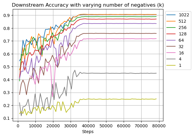
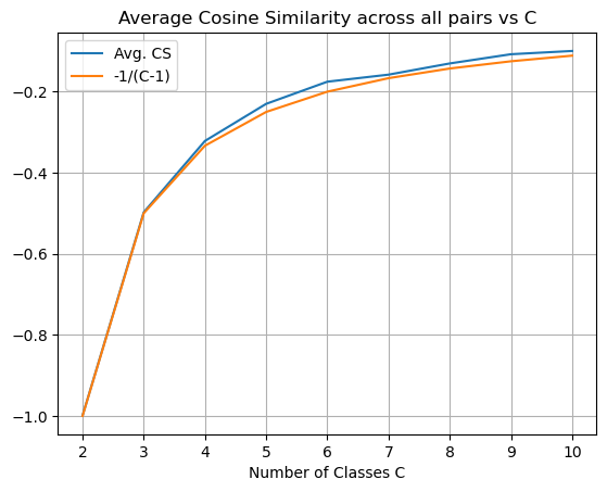
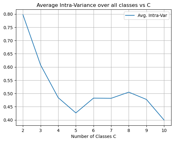
On CIFAR-10 we perform a more extensive set of experiments scaling the values of the number of negative samples $k$. We also sub-sample CIFAR-10 to contain fewer than 10 classes and investigate how the structure of the resulting representations change. In our setup, we observe a steady increase in the downstream performance all the way from $k=1$ up to $k=512$ (Figure 2). Figure 3 shows how the average $\mathsf{CS}$ and Intra-Variance_c values change with the total number of classes $C$. The average $\mathsf{CS}$ value in particular is strongly in line with what is predicted by our theory.

Figure 2: Downstream classification accuracy of contrastively learnt representations on CIFAR-10 improves with increasing the number of negative examples $k$.

Figure 3: The change in the average inter-classes cosine similarities and average intraclass variances of the representations is plotted for different values of the number of classes $C$ while the number of negative samples $k$ is fixed at 1022. Experiments were done by sub-sampling CIFAR-10 to have fewer classes. The orange line in the graph on the left plots what our theory predicts.

6 Comparing our Results with Prior Work

Here we discuss our results and their implications in context of prior work studying the impact of negative samples in contrastive learning.

Comparing with prior empirical observations.

Some empirical phenomena suggest that while more negative samples help initially, when increased beyond a certain point, they can start to hurt (Ash et al., 2022; Mitrovic et al., 2020). On the other hand, as we observe in our paper, if we analyze the representation minimizing the population NCE loss, larger number of negative samples continues to help improve the downstream supervised learning task, or at least does not hurt it. How do we then reconcile these two observations?

There are three important ways in which our analysis simplifies what happens in the real world. The first is by assuming that our optimizer (typically a variant of stochastic gradient descent) has reached a global minimum. This might not always hold in practice. In particular, the optimizer might find it harder to reach a global minima with increasing values of $k$. The second aspect is that perhaps the class of deep neural nets optimized by SGD is not expressive enough to be able to perfectly satisfy our structural characterization of the minimizer. This corresponds to the setting when there is an approximation error as we minimize among a restricted class of functions. On the other hand, if the class is highly expressive, then there remains the question of finite sample generalization of the empirical NCE optimal representation. And lastly, the positive pair generation process may be quite different to the one we considered which could lead to quite different properties of the minimizer.

Apart from these three reasons, another factor to consider is our assumption of non-overlapping latent classes which might not hold perfectly in practice leading to small inconsistencies in observed performance. Moreover, the story is not very clear on the empirical side as well. In works which report experiments showing that a large number of negative samples hurt performance beyond a point (Ash et al., 2022; Saunshi et al., 2019), the degradation in performance is quite small ($1-2\%$ drop in accuracy) and it is unclear if it cannot be attributed to noise introduced during training. Mitrovic et al. (2020) also report a small amount of degradation at higher $k$ but their positive pair generation process is different from what we consider in our setting. In addition, experiments performed in the works of Nozawa & Sato (2021); Bao et al. (2021) seem to indicate that increasing $k$ does not hurt downstream classification performance.

Comparing with prior theoretical observations.

The theoretical work closest to ours is that of (Saunshi et al., 2019; Ash et al., 2022) who work with a similar framework as ours. The main results in these works are upper bounds on the supervised loss of any representation in terms of its NCE loss. That is, they show that, for any representation function $f$,

$$\mathcal{L}_{\mathrm{sup}}(f)\leq\alpha(k,\rho)\cdot\left(\mathcal{L}_{\mathrm{NCE}}^{(k)}(f)-\tau(k)\right)\,.$$ (5)

where in the setting of uniform distribution $\rho$ over latent classes, $\alpha(k,\rho)\approxeq\frac{4\log C(C-1)\eta^{k}}{k}$ for $\eta=1+1/(C-1)>1$ and hence for large $k$, $\alpha(k,\rho)$ grows exponentially with $k$, and $\tau(k):=1-(1-\frac{1}{C})^{k}<1$. However, this is just an upper bound on the downstream performance. In contrast, our result shows that for the minimizer $f^{*}$ of the population NCE loss, $\mathcal{L}_{\mathrm{sup}}(f^{*})$ does not increase with $k$ under Assumption 3.6 and we give supporting evidence through simulations that this monotonic behavior persists even without the uniformity assumption. Moreover in Theorem C.2 (in Appendix C), we improve the above result in the case of logistic loss by showing that for any $f$,

$$\mathcal{L}_{\mathrm{sup}}(f)\leq\beta(k,\rho)\cdot\mathcal{L}_{\mathrm{NCE}}^{(k)}(f)$$

where $\beta(k,\rho)$ is in fact non-increasing in $k$ and becomes a constant for large enough $k$. We emphasize that while our result does not have the $\tau(k)$ term, it doesn’t affect the asymptotic behavior with respect to $k$, since $\tau(k)\leq 1$ whereas $\mathcal{L}_{\mathrm{NCE}}^{(k)}(f)$ increases with $k$. However, we note again that $\mathcal{L}_{\mathrm{sup}}$ (which is a classification objective over $C$ classes) has a different scale than $\mathcal{L}_{\mathrm{NCE}}^{(k)}$ (which is a classification objective over $k$ classes). In particular, $\mathcal{L}_{\mathrm{sup}}(f)$ is at most $\log C$ for a (trivial) constant representation, whereas $\mathcal{L}_{\mathrm{NCE}}^{(k)}(f)$ grows as $\sim\log k$ even for the NCE optimal representation. Hence it may not be meaningful to prove an upper bound on the downstream supervised loss of a representation directly in terms of the NCE loss, and instead study the representations that are NCE optimal (or close to one) directly as we do in this paper.

To support their proposition that a worsening of performance with increased $k$ is unavoidable, both Saunshi et al. (2019); Ash et al. (2022) present example representation functions and distributions where the representation giving better NCE loss yields a worse supervised loss. However these are not formal lower bounds on the performance of the optimal representation that minimizes the NCE loss. Indeed, our results suggest that such a formal lower bound might not exist as the performance does not degrade with $k$ (Conjecture 3.10). In addition, the examples provided in these works sometimes rely on unnormalized representations which is not what works well in practice.

After the publication of our work, we were informed about the works of Nozawa & Sato (2021); Bao et al. (2021) which provide sharper theoretical bounds for the supervised loss in terms of the contrastive loss. Bao et al. (2021) provide upper and lower bounds on the supervised loss of any representation in terms of the contrastive loss obtained on that representation. In the regime of large $k$, these upper and lower bounds differ by a constant which is independent of $C,k$. We compare and contrast these results with ours across two settings: (i) uniform class distribution: in this setting, our structural characterization in Theorem 3.8 provides an exact understanding of the downstream loss of the NCE optimal representation. On the other hand, the bounds provided in Nozawa & Sato (2021); Bao et al. (2021) (which applies to any representation) do not in particular imply that the performance of the NCE optimal representation on the downstream task does not degrade at all with increasing $k$; (ii) non-uniform class distributions: in this setting, we are not able to show that the downstream performance does not degrade with increasing $k$. The bounds in Bao et al. (2021) continues to provide a sharp characterization of the supervised loss of any representation, but as far as we know, Conjecture 3.10 remains open. At a broader level, the message in the works of (Nozawa & Sato, 2021; Bao et al., 2021) is aligned with the message in our work that more negative samples in contrastive learning do not necessarily hurt downstream performance.

To conclude, we analyzed normalized representations and see a much nicer structure emerge in the population NCE optimal representation. Our investigation suggests that the “collision-coverage” tradeoff is not sufficient on its own for explaining the non-monotonic behavior in the downstream performance as a function of the number of negative samples that is observed in practice.

Appendix A Proof of Structural Results

A.1 Non-overlapping Latent Classes

See 3.3

Proof.

We consider the case of $\beta=1$. The case of general $\beta$ follows immediately.

For $\ell_{\mathrm{log}}(v):=\log(1+\sum_{i}\exp(-v_{i}))$, using concavity of $\log$ (Jensen’s inequality), and denoting $T:=1+\sum_{j\notin S}\exp(-v_{j})$, we have

$$\textstyle\ell_{\mathrm{log}}(v)~{}=~{}\log\left(T+\sum_{i\in S}\exp(-v_{i})\right)~{}\geq~{}\frac{1}{|S|}\sum_{i\in S}\log\left(T+|S|\cdot\exp(-v_{i})\right)~{}=~{}\frac{1}{|S|}\sum_{i\in S}\ell_{\mathrm{log}}(v^{S\leftarrow i})$$

For $\ell_{\mathrm{hinge}}(v):=\max\left\{0,1+\max\left\{-v_{i}\right\}\right\}$, using the simple property that $\max\left\{a_{1},\ldots,a_{k}\right\}\geq(\sum a_{i})/k$, we have

$$\ell(v) \textstyle~{}=~{}\max\left\{0,1+\max_{i\in S}\left\{-v_{i}\right\},1+\max_{j\notin S}\left\{-v_{j}\right\}\right\}$$

$$\textstyle~{}\geq~{}\frac{1}{|S|}\sum_{i\in S}\max\left\{0,1-v_{i},1+\max_{j\notin S}\left\{-v_{j}\right\}\right\}~{}=~{}\frac{1}{|S|}\sum_{i\in S}\ell_{\mathrm{hinge}}(v^{S\leftarrow i})\qed$$

See 3.5

Proof.

We show the existence of $\widetilde{f}$ in an existential manner. For a fixed latent class $c^{*}\in\mathcal{C}$, sample $x^{*}\sim\mathcal{D}_{c^{*}}$ and define a representation $f_{x^{*}}:\mathcal{X}\to\mathbb{S}^{d-1}$ as

$$f_{x^{*}}(x) ~{}:=~{}\begin{cases}f(x^{*})&\text{if }c(x)=c^{*}\\ f(x)&\text{if }c(x)\neq c^{*}\end{cases}$$ (6)

We will show that $\operatorname*{\mathbb{E}}_{x^{*}\sim\mathcal{D}_{c}}\mathcal{L}_{\mathrm{NCE}}^{(k)}(f_{x^{*}})\leq\mathcal{L}_{\mathrm{NCE}}^{(k)}(f)$. This implies the existence of an $x^{*}$ in support of $\mathcal{D}_{c^{*}}$ such that $\mathcal{L}_{\mathrm{NCE}}^{(k)}(f_{x^{*}})\leq\mathcal{L}_{\mathrm{NCE}}^{(k)}(f)$.

We can rewrite the NCE loss as

$$\mathcal{L}_{\mathrm{NCE}}^{(k)}(f) ~{}=~{}\operatorname*{\mathbb{E}}_{c,c_{1:k}\sim\rho}\ \underbrace{\operatorname*{\mathbb{E}}_{x,x^{+}\sim\mathcal{D}_{c}}\ \operatorname*{\mathbb{E}}_{\left\langle x_{i}^{-}\sim\mathcal{D}_{c_{i}}\right\rangle}\ \ell\left(\left\langle f(x)^{\top}(f(x^{+})-f(x_{i}^{-}))\right\rangle_{i=1}^{k}\right)}_{=:~{}\mathcal{L}_{c,c_{1:k}}(f)}$$ (7)

We will show that for each $c,c_{1:k}$, it holds that $\operatorname*{\mathbb{E}}_{x^{*}\sim\mathcal{D}_{c^{*}}}\mathcal{L}_{c,c_{1:k}}(f_{x^{*}})\leq\mathcal{L}_{c,c_{1:k}}(f)$.

Case $c=c^{*}$:

For ease of notation let $c_{1},\ldots,c_{q}=c^{*}$ and $c_{q+1},\ldots,c_{k}\neq c^{*}$. We have

$$\mathcal{L}_{c,c_{1:k}}(f) ~{}=~{}\operatorname*{\mathbb{E}}_{x,x_{q+1:k}^{-}}\operatorname*{\mathbb{E}}_{x^{+},x_{1:q}^{-}}\ell\left(\left\langle f(x)^{\top}(f(x^{+})-f(x_{i}^{-}))\right\rangle_{i=1}^{k}\right)$$ (8)

$$~{}\geq~{}\operatorname*{\mathbb{E}}_{x,x_{q+1:k}^{-}}\operatorname*{\mathbb{E}}_{x^{+},x_{1:q}^{-}}\ell\left(\left\langle f(x)^{\top}(f(x^{+})-f(x_{i}^{-}))\right\rangle_{i=1}^{q}\circ\left\langle 1-f(x)^{\top}f(x_{i}^{-}))\right\rangle_{i=q+1}^{k}\right)$$ (9)

$$~{}\geq~{}\operatorname*{\mathbb{E}}_{x,x_{q+1:k}^{-}}\ell\left(\left\langle\operatorname*{\mathbb{E}}_{x^{+},x_{1:q}^{-}}f(x)^{\top}(f(x^{+})-f(x_{i}^{-}))\right\rangle_{i=1}^{q}\circ\left\langle 1-f(x)^{\top}f(x_{i}^{-}))\right\rangle_{i=q+1}^{k}\right)$$ (10)

$$~{}=~{}\operatorname*{\mathbb{E}}_{x,x_{q+1:k}^{-}}\ell\left(\left\langle 0\right\rangle_{i=1}^{q}\circ\left\langle 1-f(x)^{\top}f(x_{i}^{-}))\right\rangle_{i=q+1}^{k}\right)$$ (11)

where, (9) holds because $f(x)^{\top}f(x^{+})\leq 1$ and $\ell(v)$ is non-increasing in each $v_{i}$, (10) holds due to convexity of $\ell$ (Jensen’s inequality), and (11) holds because $\operatorname*{\mathbb{E}}_{x^{+},x_{i}^{-}\sim\mathcal{D}_{c^{*}}}[f(x^{+})-f(x_{i}^{-})]=0$. Finally, we observe that the quantity in (11) is precisely $\operatorname*{\mathbb{E}}_{x^{*}\sim\mathcal{D}_{c^{*}}}\mathcal{L}_{c,c_{1:k}}(f_{x^{*}})$, since

$$\operatorname*{\mathbb{E}}_{x^{*}\sim\mathcal{D}_{c^{*}}}\mathcal{L}_{c,c_{1:k}}(f_{x^{*}}) ~{}=~{}\operatorname*{\mathbb{E}}_{x^{*}\sim\mathcal{D}_{c^{*}}}\operatorname*{\mathbb{E}}_{x,x_{q+1:k}^{-}}\operatorname*{\mathbb{E}}_{x^{+},x_{1:q}^{-}}\ell\left(\left\langle f_{x^{*}}(x)^{\top}(f_{x^{*}}(x^{+})-f_{x^{*}}(x_{i}^{-}))\right\rangle_{i=1}^{k}\right)$$ (12)

$$~{}=~{}\operatorname*{\mathbb{E}}_{x^{*}\sim\mathcal{D}_{c^{*}}}\operatorname*{\mathbb{E}}_{x,x_{q+1:k}^{-}}\ell\left(\left\langle 0\right\rangle_{i=1}^{q}\circ\left\langle 1-f(x^{*})^{\top}f(x_{i}^{-}))\right\rangle_{i=q+1}^{k}\right)$$ (13)

which is same as the quantity in (11) up to renaming $x$ by $x^{*}$ (note: both $x,x^{*}\sim\mathcal{D}_{c^{*}}$ here). For a strictly convex loss, note that our application of Jensen’s inequality is tight only when $\Pr[f(x)^{\top}(f(x^{+})-f(x_{i}^{-}))=0]=1$, which is the case only if $\Pr_{x,x^{\prime}\sim\mathcal{D}_{c^{*}}}[f(x)=f(x^{\prime})]=1$.

Case $c\neq c^{*}$:

Again, for ease of notation let $c_{1},\ldots,c_{q}=c^{*}$ and $c_{q+1},\ldots,c_{k}\neq c^{*}$. We have

$$\mathcal{L}_{c,c_{1:k}}(f) ~{}=~{}\operatorname*{\mathbb{E}}_{x,x^{+}x_{q+1:k}^{-}}\operatorname*{\mathbb{E}}_{x_{1:q}^{-}\sim\mathcal{D}_{c^{*}}}\ell\left(\left\langle f(x)^{\top}(f(x^{+})-f(x_{i}^{-}))\right\rangle_{i=1}^{k}\right)$$ (14)

$$\operatorname*{\mathbb{E}}_{x^{*}\sim\mathcal{D}_{c^{*}}}\mathcal{L}_{c,c_{1:k}}(f_{x^{*}}) ~{}=~{}\operatorname*{\mathbb{E}}_{x,x^{+}x_{q+1:k}^{-}}\operatorname*{\mathbb{E}}_{x^{*}\sim\mathcal{D}_{c^{*}}}\ell\left(\left\langle f(x)^{\top}(f(x^{+})-f(x^{*}))\right\rangle_{i=1}^{k}\right)$$ (15)

We will show that for all $x,x^{+},x_{q+1:k}^{-}$, for any loss $\ell$ satisfying Property 3.2 it holds that

$$\operatorname*{\mathbb{E}}_{x_{1:q}^{-}\sim\mathcal{D}_{c^{*}}}\ell\left(\left\langle f(x)^{\top}(f(x^{+})-f(x_{i}^{-}))\right\rangle_{i=1}^{k}\right)~{}\geq~{}\operatorname*{\mathbb{E}}_{x^{*}\sim\mathcal{D}_{c^{*}}}\ell\left(\left\langle f(x)^{\top}(f(x^{+})-f(x^{*}))\right\rangle_{i=1}^{k}\right)$$

For ease of notation, consider a random variable $Z$ that is distributed as $f(x)^{\top}(f(x^{+})-f(x^{-}))$ for $x^{-}\sim\mathcal{D}_{c^{*}}$ (for fixed $x$ and $x^{+}$). For any loss $\ell$ satisfying Property 3.2, we have that

$$\operatorname*{\mathbb{E}}_{Z_{1:q}}\ \ell\left(\left\langle Z_{i}\right\rangle_{i=1}^{q}\circ\left\langle f(x)^{\top}(f(x^{+})-f(x_{i}^{-}))\right\rangle_{i=q+1}^{k}\right)$$

$$~{}\geq~{}\operatorname*{\mathbb{E}}_{Z_{1:q}}\left[\frac{1}{q}\sum_{j=1}^{k}\ell\left(\left\langle Z_{j}\right\rangle_{i=1}^{q}\circ\left\langle f(x)^{\top}(f(x^{+})-f(x_{i}^{-}))\right\rangle_{i=q+1}^{k}\right)\right]$$

$$~{}=~{}\operatorname*{\mathbb{E}}_{Z}\ \ell\left(\left\langle Z\right\rangle_{i=1}^{q}\circ\left\langle f(x)^{\top}(f(x^{+})-f(x_{i}^{-}))\right\rangle_{i=q+1}^{k}\right)$$

Thus, we have $\operatorname*{\mathbb{E}}_{x^{*}\sim\mathcal{D}_{c^{*}}}\mathcal{L}_{\mathrm{NCE}}^{(k)}(f_{x^{*}})\leq\mathcal{L}_{\mathrm{NCE}}^{(k)}(f)$, thereby completing the proof. The existence of $\widetilde{f}$ follows by iteratively repeating this argument for each latent class $c^{*}\in\mathcal{C}$.

Moreover, if $\ell$ is strictly convex loss and $f$ is not latent-indistinguishable, then we have a strict inequality in the case of $c=c^{*}$ for at least one $c^{*}$ in this iterative process. Thus, in the case of a strictly convex loss $\ell$, the only NCE optimal representations are almost latent-indistinguishable. ∎

A.2 Uniform distribution over classes

See 3.9

Proof.

We prove the statement for latent-indistinguishable representations $f$. The proof for almost latent-indistinguishable representations follows similarly.

Let $u_{c}$ denote the (common) representation for all $x$ in latent class $c$, namely $f(x)=u_{c(x)}$. Observe that $\|\sum_{c\in\mathcal{C}}u_{c}\|_{2}^{2}=C+\sum_{c\neq c^{\prime}}u_{c}^{\top}u_{c^{\prime}}\geq 0$ and hence $\operatorname*{\mathbb{E}}_{c,c^{\prime}\sim\rho}[u_{c}^{\top}u_{c^{\prime}}\mid c\neq c^{\prime}]\geq-1/(C-1)$ (under Assumption 3.6 that $\rho$ is uniform over $\mathcal{C}$). Let $\widetilde{f}$ be an equiangular representation given as $\widetilde{f}(x)=\widetilde{u}_{c(x)}$ satisfying

$$\widetilde{u}_{c}^{\top}\widetilde{u}_{c^{\prime}}=\begin{cases}1&\text{if }c=c^{\prime}\\ \operatorname*{\mathbb{E}}_{c,c^{\prime}\sim\rho}[u_{c}^{\top}u_{c^{\prime}}\mid c\neq c^{\prime}]&\text{if }c\neq c^{\prime}\end{cases}\,.$$

We will show that $\mathcal{L}_{\mathrm{NCE}}^{(k)}(\widetilde{f})\leq\mathcal{L}_{\mathrm{NCE}}^{(k)}(f)$ for any convex loss $\ell$. Observe that since $f$ and $\widetilde{f}$ are latent-indistinguishable, we can write $\mathcal{L}_{\mathrm{NCE}}^{(k)}(f)$ in the following simplified form

$$\mathcal{L}_{\mathrm{NCE}}^{(k)}(f)~{}=~{}\operatorname*{\mathbb{E}}\limits_{c,c_{1},\ldots,c_{k}\sim\rho}\ \left[\ell(1-u_{c}^{\top}u_{c_{1}},1-u_{c}^{\top}u_{c_{2}},\ldots,1-u_{c}^{\top}u_{c_{k}})\right]$$

For any permutation $\pi$ over $\mathcal{C}$, let $f_{\pi}$ denote the representation obtained by permuting the representations of the latent classes, namely, $f_{\pi}(x)~{}:=~{}u_{\pi(c(x))}$. We have the following

$$\mathcal{L}_{\mathrm{NCE}}^{(k)}(f) ~{}=~{}\operatorname*{\mathbb{E}}_{\pi}\left[\mathcal{L}_{\mathrm{NCE}}^{(k)}(f_{\pi})\right]$$

$$~{}=~{}\operatorname*{\mathbb{E}}\limits_{c,c_{1},\ldots,c_{k}\sim\rho}\operatorname*{\mathbb{E}}_{\pi}\ \left[\ell(1-u_{\pi(c)}^{\top}u_{\pi(c_{1})},1-u_{\pi(c)}^{\top}u_{\pi(c_{2})},\ldots,1-u_{\pi(c)}^{\top}u_{\pi(c_{k})})\right]$$

$$~{}\geq~{}\operatorname*{\mathbb{E}}\limits_{c,c_{1},\ldots,c_{k}\sim\rho}\ \left[\ell(1-\operatorname*{\mathbb{E}}_{\pi}[u_{\pi(c)}^{\top}u_{\pi(c_{1})}],1-\operatorname*{\mathbb{E}}[u_{\pi(c)}^{\top}u_{\pi(c_{2})}],\ldots,1-\operatorname*{\mathbb{E}}_{\pi}[u_{\pi(c)}^{\top}u_{\pi(c_{k})}])\right]$$

$$~{}=~{}\operatorname*{\mathbb{E}}\limits_{c,c_{1},\ldots,c_{k}\sim\rho}\ \left[\ell(1-\widetilde{u}_{c}^{\top}\widetilde{u}_{c_{1}},1-\widetilde{u}_{c}^{\top}\widetilde{u}_{c_{2}},\ldots,1-\widetilde{u}_{c}^{\top}\widetilde{u}_{c_{k}})\right]$$

$$~{}=~{}\mathcal{L}_{\mathrm{NCE}}^{(k)}(\widetilde{f})$$

where the third step follows from Jensen’s inequality, using convexity of $\ell$.

Finally, for any non-increasing loss $\ell$, it is easy to see that among all equiangular representations, the representation minimizing $\mathcal{L}_{\mathrm{NCE}}^{(k)}(\cdot)$ is a Simplex ETF. Moreover, when $\ell$ is strictly convex our application of Jensen’s inequality is strict unless $u_{c}^{\top}u_{c^{\prime}}$ is the same for all $c\neq c^{\prime}$, in other words, the representation is equiangular. ∎

Appendix B More Details about the CIFAR-10/100 Experiments

We describe our experimental setup in full detail. For most of our experiments we train with a ResNet-18 (He et al., 2016) backbone and a 2-layer projection head affixed on top of it with a ReLU in the middle. The training setup closely follows that of Chen et al. (2020). We do not use any weight decay as it might bias us away from seeing a simplex ETF structure. We train using the logistic form of NCE loss and use LARS optimizer (You et al., 2017) with a batch size of $512$, learning rate of $0.2$ which is decayed using a cosine decay after $10$ warmup epochs. Departing from the setting of Chen et al. (2020), the final output of the projection head is taken as the representation as this is the vector which is used in computing the loss. This is a $128$ dimensional vector which is normalized to lie inside the unit $\ell_{2}$ ball.

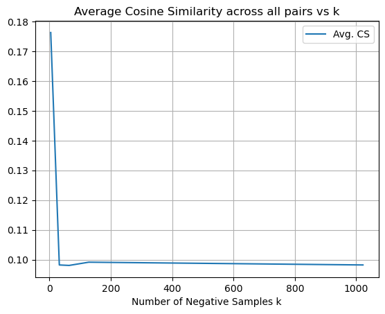
In addition to the results listed in Section 5, we present a few additional observations here. In Table 1 we present the cosine similarities matrix for a run with 5 classes. In Figure 4 we show how the average $\mathsf{CS}$ and $\mathsf{Intra}\text{-}\mathsf{Var}_{c}$ values scale with the number of negative samples for a fixed batch size.

Figure 4: The change in the average cosine similarities is plotted for different values of the number of negative samples $k$. All experiments are done for CIFAR-10 with total number of classes=10.

1.0	-0.156	-0.204	-0.342	-0.3413
-0.156	1.0	-0.373	-0.343	-0.327
-0.204	-0.373	1.0	-0.126	0.06
-0.342	-0.343	-0.126	1.0	-0.173
-0.3413	-0.327	0.06	-0.173	1.0

Table 1: The cosine similarities between the mean representations of different classes. Shown here for contrastive learning run on a subset of 5 classes from CIFAR-10. Diagonal values are always $1.0$. Our theory expects the off diagonal entries to be $-0.25$

Appendix C Improving Theorem 5 of Ash et al. (2022)

In our work, we showed that in the case of uniform latent classes, the NCE optimal representation doesn’t get worse with $k$ in terms of the downstream classification error. However, we could also try to upper bound the $\mathcal{L}_{\mathrm{sup}}(f)$ by some factor $G$ times the $\mathcal{L}_{\mathrm{NCE}}^{(k)}(f)$ for any representation $f$. This is precisely the form of the result obtained by Ash et al. (2022); Saunshi et al. (2019). In both these works the factor $G$ grows exponentially in $k$. We show that in the case of logistic loss, we can improve this to a factor that is non-increasing and in fact becomes a constant for large enough $k$.

We use the vector $\rho$ to denote the class distribution and $\rho_{\max}=\max\rho_{i}$ and $\rho_{\min}=\min\rho_{i}$. Here we first re-state Theorem 5 of (Ash et al., 2022) using our notation and then proceed to show a stronger result for the setting of $k\geq\rho_{\min}$ when we work with the logistic loss. Recall that in this setting, $1/(1-\rho_{\max})^{k}$ from their theorem grows exponentially in $k$ suggesting that for large values of $k$, a small $\mathcal{L}_{\mathrm{NCE}}^{(k)}(f)$ may not correspond to a small $\mathcal{L}_{\mathrm{sup}}(f)$. We will show a drastic improvement on this exponential growth with respect to $k$.

Theorem C.1 (Restatement of Theorem 5 of (Ash et al., 2022)).

For the logistic loss and any representation $f:\mathcal{X}\to\mathbb{S}^{d-1}$,

$$\mathcal{L}_{\mathrm{sup}}(f)\leq\frac{2\max\left(1,\frac{2(1-\rho_{\min})\log C}{k\rho_{\min}}\right)}{(1-\rho_{\max})^{k}}\left(\mathcal{L}_{\mathrm{NCE}}^{(k)}(f)-\tau_{k}\operatorname*{\mathbb{E}}_{c,c_{i}^{-}\sim\rho^{k+1}}\left[\log\left(1+|I|\right)|I\neq\phi\right]\right)\,,$$

where $I$ is the set of collisions among the $k$ negative samples.

We prove an improved version of Theorem C.1 below. Note that we don’t have the $\tau_{k}\operatorname*{\mathbb{E}}_{c,c_{i}^{-}\sim\rho^{k+1}}\left[\log\left(1+|I|\right)|I\neq\phi\right]$ term but the coefficient in front is vastly improved from $\frac{2\max\left(1,\frac{2(1-\rho_{\min})\log C}{k\rho_{\min}}\right)}{(1-\rho_{\max})^{k}}$ to $4\max\left(1,\frac{2(1-\rho_{\min})\log C}{k(1-\rho_{\max})\rho_{\min}}\right)$.

Theorem C.2 (Improved Theorem 5 of (Ash et al., 2022)).

Let $k\geq 1/\rho_{\max}$. For the logistic loss, for any $f:\mathcal{X}\to\mathbb{S}^{d-1}$,

$$\mathcal{L}_{\mathrm{sup}}(f)~{}\leq~{}4\max\left(1,\frac{2(1-\rho_{\min})\log C}{k(1-\rho_{\max})\rho_{\min}}\right)\cdot\mathcal{L}_{\mathrm{NCE}}^{(k)}(f)\,.$$

Proof.

We recall the sub-addivitity property of logistic loss.

Lemma C.3 (Sub-additivity of Logistic Loss (Lemma 1, (Ash et al., 2022))).

Let $v\in\mathbb{R}^{k}$ be a vector. For all $I_{1},I_{2}\subset[k]$, and $S=I_{1}\cup I_{2}$, we have that

$$\ell(\{v_{i}\}_{i\in I_{1}})~{}\leq~{}\ell(\{v_{i}\}_{i\in S})~{}\leq~{}\ell(\{v_{i}\}_{i\in I_{1}})+\ell(\{v_{i}\}_{i\in I_{2}})\,.$$

Following (Ash et al., 2022), we begin with an application of Jensen’s inequality to get

$$\mathcal{L}_{\mathrm{NCE}}^{(k)}(f) ~{}=~{}\operatorname*{\mathbb{E}}_{\mathcal{D}_{\mathrm{NCE}}}\left[\ell\left(\left\langle f(x)^{\top}(f(x^{+})-f(x_{i}^{-}))\right\rangle_{i=1}^{k}\right)\right]\,$$

$$~{}\geq~{}\operatorname*{\mathbb{E}}_{c,c_{i}^{-}\sim\rho^{k+1},x\sim D_{c}}\left[\ell\left(\left\langle f(x)^{\top}(\mu_{c}-\mu_{c_{i}^{-}})\right\rangle_{i=1}^{k}\right)\right]\,,$$ (16)

where $\mu_{c}=\operatorname*{\mathbb{E}}_{x\sim D_{c}}[f(x)]$. Given $k$ negative samples, if the last $k_{1}$ of them are collisions, we have from the sub-additivity of the logistic loss,

$$\ell\left(\left\langle f(x)^{\top}\left(\mu_{c}-\mu_{c_{i}}^{-}\right)\right\rangle_{i=1}^{k}\right) ~{}=~{}\ell\left(\left\langle f(x)^{\top}\left(\mu_{c}-\mu_{c_{i}}^{-}\right)\right\rangle_{i=1}^{k-k_{1}}\circ\left\langle 0\right\rangle_{i=k-k_{1}+1}^{k}\right)~{}\geq~{}\ell\left(\left\langle f(x)^{\top}\left(\mu_{c}-\mu_{c_{i}}^{-}\right)\right\rangle_{i=1}^{k-k_{1}}\right).$$ (17)

Now for any fixed $c$, the probability of a collision for a randomly drawn negative sample is $\rho_{c}$. Given $k$ negative samples, let $I_{c}$ denote the set of collisions among the negative samples. For simplicity, we will assume that $k\rho_{\max}$ is an integer. For the most likely class, $|I_{\max}|$ is distributed as $\mathrm{Bin}(k,\rho_{\max})$ and its median is precisely $k\rho_{\max}$. Therefore, we have that

$$\Pr\left[|I_{\max}|>k\rho_{\max}\right]\leq 1/2\,.$$ (18)

Let $k^{\prime}=k(1-\rho_{\max})$. Now,

$$\mathcal{L}_{\mathrm{NCE}}^{(k)}(f) ~{}\geq~{}\operatorname*{\mathbb{E}}_{c,c_{i}^{-},x\sim D_{c}}\left[\ell\left(\left\langle f(x)^{\top}(\mu_{c}-\mu_{c_{i}^{-}})\right\rangle_{i=1}^{k}\right)\right]$$

$$~{}=~{}\operatorname*{\mathbb{E}}_{c\sim\rho}\left[\Pr\left[|I_{c}|\leq k\rho_{\max}\right]\cdot\operatorname*{\mathbb{E}}_{c_{i}^{-}\sim\rho^{k},x\sim D_{c}}\left[\ell\left(\left\langle f(x)^{\top}(\mu_{c}-\mu_{c_{i}^{-}})\right\rangle_{i=1}^{k}\right)\,\Big{|}\,|I_{c}|\leq k\rho_{\max}\right]\right]$$

$$~{}~{}~{}~{}~{}+\operatorname*{\mathbb{E}}_{c\sim\rho}\left[\Pr\left[|I_{c}|>k\rho_{\max}\right]\cdot\operatorname*{\mathbb{E}}_{c_{i}^{-}\sim\rho^{k},x\sim D_{c}}\left[\ell\left(\left\langle f(x)^{\top}(\mu_{c}-\mu_{c_{i}^{-}})\right\rangle_{i=1}^{k}\right)\,\Big{|}\,|I_{c}|>k\rho_{\max}\right]\right]$$

$$~{}\geq~{}\operatorname*{\mathbb{E}}_{c\sim\rho}\left[\Pr\left[|I_{c}|\leq k\rho_{\max}\right]\cdot\operatorname*{\mathbb{E}}_{c_{i}^{-}\sim\rho_{-c}^{k^{\prime}},x\sim D_{c}}\left[\ell\left(\left\langle f(x)^{\top}(\mu_{c}-\mu_{c_{i}^{-}})\right\rangle_{i=1}^{k^{\prime}}\right)\right]\right]$$ (19)

$$~{}\geq~{}\Pr\left[|I_{\max}|\leq k\rho_{\max}\right]\cdot\operatorname*{\mathbb{E}}_{c\sim\rho,c_{i}^{-}\sim\rho_{-c}^{k^{\prime}},x\sim D_{c}}\left[\ell\left(\left\langle f(x)^{\top}(\mu_{c}-\mu_{c_{i}^{-}})\right\rangle_{i=1}^{k^{\prime}}\right)\right]\,.$$ (20)

Next, we use Lemma 4 from (Ash et al., 2022) which gives that for any $c\in\mathcal{C}$ and any $x$

$$\operatorname*{\mathbb{E}}_{c_{i}^{-}\sim\rho_{-c}^{k^{\prime}}}\left[\ell\left(\left\langle f(x)^{\top}(\mu_{c}-\mu_{c_{i}^{-}})\right\rangle_{i=1}^{k^{\prime}}\right)\right]~{}\geq~{}\frac{1}{2\left\lceil\frac{2(1-\rho(c))\log C}{(k^{\prime})\min_{c^{\prime}\neq c}\rho(c^{\prime})}\right\rceil}\cdot\ell\left(\left\langle f(x)^{\top}(\mu_{c}-\mu_{c^{\prime}})\right\rangle_{c^{\prime}\in\mathcal{C}\backslash\{c\}}\right).$$ (21)

Substituting these above, we get

$$\mathcal{L}_{\mathrm{NCE}}^{(k)}(f) \geq\frac{1}{2}\operatorname*{\mathbb{E}}_{c\sim D,c_{i}^{-}\sim D_{-c}^{k^{\prime}},x\sim D_{c}}\left[\ell\left(\left\langle f(x)^{\top}(\mu_{c}-\mu_{c_{i}^{-}})\right\rangle_{i=1}^{k^{\prime}}\right)\right]$$ (22)

$$\geq\frac{1}{2}\operatorname*{\mathbb{E}}_{c\sim D}\frac{1}{2\left\lceil\frac{2(1-\rho_{\min})\log C}{(k^{\prime})\rho_{\min}}\right\rceil}\cdot\ell\left(\left\langle f(x)^{\top}(\mu_{c}-\mu_{c^{\prime}})\right\rangle_{c^{\prime}\in\mathcal{C}\backslash\{c\}}\right)$$ (23)

$$\geq\frac{1}{4\left\lceil\frac{2(1-\rho_{\min})\log C}{(k^{\prime})\rho_{\min}}\right\rceil}\cdot\mathcal{L}_{\mathrm{sup}}(f,\left\langle\mu_{c}\right\rangle_{c\in\mathcal{C}})$$ (24)

$$\geq\frac{1}{4\left\lceil\frac{2(1-\rho_{\min})\log C}{(k^{\prime})\rho_{\min}}\right\rceil}\cdot\mathcal{L}_{\mathrm{sup}}(f)$$ (25)

which gives us the claimed result. ∎

References

- Ash et al. (2022) Ash, J. T., Goel, S., Krishnamurthy, A., and Misra, D. Investigating the role of negatives in contrastive representation learning. In The 25th International Conference on Artificial Intelligence and Statistics, AISTATS 2022, Proceedings of Machine Learning Research. PMLR, 2022. URL https://arxiv.org/abs/2106.09943.
- Bao et al. (2021) Bao, H., Nagano, Y., and Nozawa, K. Sharp learning bounds for contrastive unsupervised representation learning. arXiv preprint arXiv:2110.02501, 2021.
- Bengio et al. (2013) Bengio, Y., Courville, A., and Vincent, P. Representation learning: A review and new perspectives. IEEE transactions on pattern analysis and machine intelligence, 35(8):1798–1828, 2013.
- Chen & Li (2020) Chen, T. and Li, L. Intriguing properties of contrastive losses. arXiv preprint arXiv:2011.02803, 2020.
- Chen et al. (2020) Chen, T., Kornblith, S., Norouzi, M., and Hinton, G. A simple framework for contrastive learning of visual representations. In International conference on machine learning, pp. 1597–1607. PMLR, 2020.
- Clark et al. (2020) Clark, K. L., Le, M., Manning, Q., and ELECTRA, C. Pre-training text encoders as discriminators rather than generators. Preprint at https://arxiv. org/abs/2003.10555, 2020.
- Coates & Ng (2012) Coates, A. and Ng, A. Y. Learning feature representations with k-means. In Neural networks: Tricks of the trade, pp. 561–580. Springer, 2012.
- Devlin et al. (2018) Devlin, J., Chang, M.-W., Lee, K., and Toutanova, K. Bert: Pre-training of deep bidirectional transformers for language understanding. arXiv preprint arXiv:1810.04805, 2018.
- Grill et al. (2020) Grill, J.-B., Strub, F., Altché, F., Tallec, C., Richemond, P. H., Buchatskaya, E., Doersch, C., Pires, B. A., Guo, Z. D., Azar, M. G., et al. Bootstrap your own latent: A new approach to self-supervised learning. arXiv preprint arXiv:2006.07733, 2020.
- Gutmann & Hyvärinen (2010) Gutmann, M. and Hyvärinen, A. Noise-contrastive estimation: A new estimation principle for unnormalized statistical models. In Proceedings of the thirteenth international conference on artificial intelligence and statistics, pp. 297–304. JMLR Workshop and Conference Proceedings, 2010.
- HaoChen et al. (2021) HaoChen, J. Z., Wei, C., Gaidon, A., and Ma, T. Provable guarantees for self-supervised deep learning with spectral contrastive loss. In Advances in Neural Information Processing Systems, 2021. URL https://openreview.net/forum?id=mjyMGFL8N2.
- He et al. (2016) He, K., Zhang, X., Ren, S., and Sun, J. Deep residual learning for image recognition. In Proceedings of the IEEE conference on computer vision and pattern recognition, pp. 770–778, 2016.
- Higham (2002) Higham, N. J. Computing the nearest correlation matrix—a problem from finance. IMA Journal of Numerical Analysis, 22(3):329–343, 2002. doi: 10.1093/imanum/22.3.329.
- Krizhevsky et al. (2009) Krizhevsky, A., Hinton, G., et al. Learning multiple layers of features from tiny images. 2009.
- Lacoste-Julien et al. (2012) Lacoste-Julien, S., Schmidt, M., and Bach, F. R. A simpler approach to obtaining an o(1/t) convergence rate for the projected stochastic subgradient method. CoRR, abs/1212.2002, 2012. URL http://arxiv.org/abs/1212.2002.
- Lee & Seung (1999) Lee, D. D. and Seung, H. S. Learning the parts of objects by non-negative matrix factorization. Nature, 401(6755):788–791, 1999.
- Mairal et al. (2009) Mairal, J., Bach, F., Ponce, J., and Sapiro, G. Online dictionary learning for sparse coding. In Proceedings of the 26th annual international conference on machine learning, pp. 689–696, 2009.
- Mikolov et al. (2013) Mikolov, T., Chen, K., Corrado, G., and Dean, J. Efficient estimation of word representations in vector space. arXiv preprint arXiv:1301.3781, 2013.
- Mitrovic et al. (2020) Mitrovic, J., McWilliams, B., and Rey, M. Less can be more in contrastive learning. 2020.
- Nozawa & Sato (2021) Nozawa, K. and Sato, I. Understanding negative samples in instance discriminative self-supervised representation learning. Advances in Neural Information Processing Systems, 34, 2021.
- Oord et al. (2018) Oord, A. v. d., Li, Y., and Vinyals, O. Representation learning with contrastive predictive coding. arXiv preprint arXiv:1807.03748, 2018.
- Papyan et al. (2020) Papyan, V., Han, X., and Donoho, D. L. Prevalence of neural collapse during the terminal phase of deep learning training. Proceedings of the National Academy of Sciences, 117(40):24652–24663, 2020.
- Pennington et al. (2014) Pennington, J., Socher, R., and Manning, C. D. Glove: Global vectors for word representation. In Proceedings of the 2014 conference on empirical methods in natural language processing (EMNLP), pp. 1532–1543, 2014.
- Saunshi et al. (2019) Saunshi, N., Plevrakis, O., Arora, S., Khodak, M., and Khandeparkar, H. A theoretical analysis of contrastive unsupervised representation learning. In International Conference on Machine Learning, pp. 5628–5637. PMLR, 2019.
- Saunshi et al. (2022) Saunshi, N., Ash, J. T., Goel, S., Misra, D., Zhang, C., Arora, S., Kakade, S. M., and Krishnamurthy, A. Understanding contrastive learning requires incorporating inductive biases. CoRR, abs/2202.14037, 2022. URL https://arxiv.org/abs/2202.14037.
- Schroff et al. (2015) Schroff, F., Kalenichenko, D., and Philbin, J. Facenet: A unified embedding for face recognition and clustering. In IEEE Conference on Computer Vision and Pattern Recognition (CVPR), pp. 815–823, 2015. doi: 10.1109/CVPR.2015.7298682.
- Smith & Eisner (2005) Smith, N. A. and Eisner, J. Contrastive estimation: Training log-linear models on unlabeled data. In Proceedings of the 43rd Annual Meeting of the Association for Computational Linguistics (ACL’05), pp. 354–362, 2005.
- Tian et al. (2021) Tian, Y., Chen, X., and Ganguli, S. Understanding self-supervised learning dynamics without contrastive pairs. arXiv preprint arXiv:2102.06810, 2021.
- van Lint & Seidel (1966) van Lint, J. H. and Seidel, J. J. Equilateral point sets in elliptic geometry. Indag. Math, 28(3):335–34, 1966.
- von Kügelgen et al. (2021) von Kügelgen, J., Sharma, Y., Gresele, L., Brendel, W., Schölkopf, B., Besserve, M., and Locatello, F. Self-supervised learning with data augmentations provably isolates content from style. arXiv preprint arXiv:2106.04619, 2021.
- Wang & Isola (2020) Wang, T. and Isola, P. Understanding contrastive representation learning through alignment and uniformity on the hypersphere. In International Conference on Machine Learning, pp. 9929–9939. PMLR, 2020.
- Wang et al. (2021) Wang, X., Zhang, R., Shen, C., Kong, T., and Li, L. Dense contrastive learning for self-supervised visual pre-training. In Proceedings of the IEEE/CVF Conference on Computer Vision and Pattern Recognition, pp. 3024–3033, 2021.
- You et al. (2017) You, Y., Gitman, I., and Ginsburg, B. Large batch training of convolutional networks. arXiv preprint arXiv:1708.03888, 2017.
- Zimmermann et al. (2021) Zimmermann, R. S., Sharma, Y., Schneider, S., Bethge, M., and Brendel, W. Contrastive learning inverts the data generating process. arXiv preprint arXiv:2102.08850, 2021.