The time-dependent harmonic oscillator revisited

Abstract

We re-examine the time-dependent harmonic oscillator $\ddot{q}=-\omega^{2}q$ under various regularity assumptions. Where $\omega(t)$ is continuously differentiable we reduce its integration to that of a single first order equation, i.e. the Hamilton equation for the angle variable $\psi$ alone (the action variable ${\cal I}$ does not appear). Reformulating the generic Cauchy problem for $\psi(t)$ as a Volterra-type integral equation and applying the fixed point theorem we obtain a sequence $\{\psi^{(h)}\}_{h\in\mathbb{N}_{0}}$ converging uniformly to $\psi$ in every compact time interval; if $\omega$ varies slowly or little, already $\psi^{(0)}$ approximates $\psi$ well for rather long time lapses. The discontinuities of $\omega$, if any, determine those of $\psi,{\cal I}$. The zeroes of $q,\dot{q}$ are investigated with the help of two Riccati equations. As a demo of the potential of our approach, we briefly argue that it yields good approximations of the solutions (as well as exact bounds on them) and thereby may simplify the study of: the stability of the trivial one; the occurrence of parametric resonance when $\omega(t)$ is periodic; the adiabatic invariance of ${\cal I}$; the asymptotic expansions in a slow time parameter $\varepsilon$; etc.

1 Introduction

The equation of the time-dependent harmonic oscillator

$$\ddot{q}(t)=-\omega^{2}(t)q(t),\qquad\omega(t)>0$$ (1)

(we abbreviate $\dot{f}\equiv df/dt$, etc.) has countless applications in natural sciences. In physics, it arises e.g. in classical and quantum mechanics, optics, electronics, electrodynamics, plasma physics, astronomy, geo- and astro-physics, cosmology (see e.g. [18, 20, 25, 31, 11, 22, 19, 3, 32, 4, 11, 24, 1]), possibly after reduction from more general equations. Moreover, in the equivalent form of Hamilton equations  $\dot{q}=p$,  $\dot{p}=-\omega^{2}q$  associated to the Hamiltonian

$$H(q,p;t):=\frac{1}{2}\left[p^{2}+\omega^{2}(t)q^{2}\right]$$ (2)

it is paradigmatic for investigating general phenomena in non-autonomous Hamiltonian systems, such as: i) the long-time behaviour of the solutions and of the adiabatic invariants under slow or small time-dependences; ii) the characterization of the time-dependences making the trivial solution unstable; in particular, iii) the characterization of the periodic ones leading to periodic solutions or to parametric resonance; iv) the behaviour of solutions under fast or large time-dependences; etc. Moreover, known two independent solutions of (1) we can find the general solution of a linear equation of the form

$$\dot{x}=Ax+a,\qquad A=\left(\!\begin{array}[]{cc}0&1\\ -\omega^{2}&0\end{array}\!\right),\quad a=\left(\!\!\begin{array}[]{l}a^{1}\\ a^{2}\end{array}\!\!\right),\quad x=\left(\!\!\begin{array}[]{l}x^{1}\\ x^{2}\end{array}\!\!\right)$$ (9)

with assigned $a(t)$, $\omega^{2}(t)$ and unknown $x(t)$. In [8] we use a family of equations of this type to describe the evolution of the Jacobian relating the Eulerian to the Lagrangian variables in a family of (1+1)-dimensional models describing the impact of a very short and intense laser pulse into a cold diluted plasma; incidentally, this has given us the initial motivation for the present study. Actually, one can reduce (see section 2) the resolution of (9a) with a more general matrix $A$ to finding two independent solutions (1) with a related $\omega^{2}$.

Here we present a rather general and effective method for approximating the solutions (1), as well as a number of useful bounds or qualitative properties of the latter, that we have not been able to find in the very broad literature (see e.g. the already cited references, the more mathematical ones [7, 28, 16, 23, 21, 34, 32, 27, 30, 35, 10, 29, 17, 2], and the references therein) on the subject. Our key observation is that, passing (section 4.1) from the canonical coordinates $q,p$ to the angle-action variables $\psi,{\cal I}=H/\omega$, via

$$q=\sqrt{\frac{2{\cal I}}{\omega}}\,\sin\psi,\qquad p=\sqrt{2{\cal I}\omega}\,\cos\psi,$$ (10)

the Hamilton equations for $\psi,{\cal I}$

$$\dot{\psi}=\omega+\frac{\dot{\omega}}{2\omega}\sin(2\psi),\qquad\frac{\dot{\cal I}}{{\cal I}}=-\frac{\dot{\omega}}{\omega}\cos(2\psi)$$ (11)

are such that the first is decoupled from the second. This apparently overlooked feature of the harmonic oscillator, among the time-dependent Hamiltonian systems admitting angle-action variables, is at the basis of our approach: we reduce (1) to (11a); afterwards (11b) is solved by quadrature. Reformulating the generic Cauchy problem (11a) with $\psi(t_{*})=\psi_{*}$ as an integral equation and applying the fixed point theorem (section 4.2) we obtain a sequence $\{\psi^{(h)}\}_{h\in\mathbb{N}_{0}}$ such that $|\psi\!-\!\psi^{(h)}|$ - and therefore also the corresponding $|{\cal I}\!-\!{\cal I}^{(h)}|$, $|q\!-\!q^{(h)}|$, $|p\!-\!p^{(h)}|$ - uniformly go to zero in every compact interval containing $t_{*}$. If $\omega(t)$ has slow or small variations, namely if

$$\zeta:=\dot{\omega}/\omega^{2}$$ (12)

($\zeta$ is a dimensionless function measuring the relative variation of $\omega$ in the characteristic time $1/\omega$) fulfills $|\zeta|\ll 1$, then already the 0-th order (in $\zeta$) approximation

$$\begin{array}[]{ll}{\cal I}^{(0)}(t)={\cal I}_{*}:={\cal I}(t_{*}),&\displaystyle\psi^{(0)}(t)=\psi_{*}+\!\int^{t}_{t_{*}}\!\!\!dz\>\omega(z),\\[10.0pt] \displaystyle q^{(0)}=\sqrt{\frac{2{\cal I}_{*}}{\omega}}\,\sin\!\left[\psi^{(0)}\right],&\displaystyle p^{(0)}=\sqrt{2{\cal I}_{*}\omega}\,\cos\!\left[\psi^{(0)}\right]=\dot{q}^{(0)},\end{array}$$ (15)

is pretty good for quite long time intervals containing $t_{*}$, and much better than the one

$$\tilde{q}(t):=\sqrt{\!\frac{2{\cal I}_{*}}{\omega_{*}}}\sin\!\left[\psi_{*}\!+\!\omega(t)(t\!-\!t_{*})\right],\qquad\dot{\tilde{q}}(t)=[\omega(t)\!+\!\dot{\omega}(t)(t\!-\!t_{*})]\sqrt{\!\frac{2{\cal I}_{*}}{\omega_{*}}}\cos\!\left[\psi_{*}\!+\!\omega(t)(t\!-\!t_{*})\right]$$ (16)

obtained from the solution of (1) with constant $\omega\equiv\omega_{*}:=\omega(t_{*})$ by the naive substitution $\omega_{*}\mapsto\omega(t)$; for shorter time lapses (15) gives a reasonable approximation also if $\omega$ varies not so slow nor little, see fig.s 2, 3, for examples. Eq. (11) make sense in intervals where $\omega$ is continuously differentiable (or is so piecewise, while keeping continuous and with bounded derivative); but all solution $\big{(}\psi,{\cal I}\big{)}$ can be extended across the discontinuities of $\omega$ (if any) via related matching conditions.

The plan of the paper, beside section 4, is as follows. In section 2, while fixing the notation, we recall for which $A$, and how, (9) can be reduced to a homogeneous system $\dot{u}=Au$ with $A$ of the form (9b), i.e. (setting $q=u^{1}$) to (1). In section 3 we prove that if $\inf_{t\in\mathbb{R}}\{\omega(t)\}>0$ then each solution $t\in\mathbb{R}\mapsto q(t)\in\mathbb{R}$ admits a sequence $\{t_{h}\}_{h\in\mathbb{Z}}\subset\mathbb{R}$ of interlacing zeroes of $q,\dot{q}$, and we study how these $t_{h}$ depend on the initial condition fulfilled by $q(t)$; rather than via (11), we do this by reducing (1) patch by patch to a Riccati equation, which is well-defined also if $\omega$ is not continuous. In section 5 we sketch how our approach may help for several purposes: proving the adiabatic invariance of ${\cal I}$ (section 5.1) faster; determining the asymptotic expansions of $\psi,{\cal I}$ in a slow time parameter $\varepsilon$ (section 5.2) faster; determining upper/lower bounds on the solutions (section 5.3); studying the stability of the trivial one, or the occurrence of parametric resonance in the case of a periodic $\omega(t)$ (section 5.4). In section 6 we summarize our results, compare them to the literature, list some possible domains of application, point out open problems and directions for further investigations. When possible we have concentrated tedious proofs in the appendix 7.

2 Preliminaries

For generic $a,A$, the solution of the Cauchy problem (9) with $x(t_{*})\!=\!x_{*}$ can be expressed as

$$x(t)={\sf V}(t,t_{*})\left[x_{*}+\int^{t}_{t_{*}}\!dz\>{\sf V}^{-1}(z,t_{*})a(z)\right],$$ (17)

where ${\sf V}(t,t_{*})$ is the (non-degenerate) family (parametrized by $t_{*}$) of $2\!\times\!2$ matrix solutions of $\dot{V}=AV$ fulfilling ${\sf V}(t_{*},t_{*})=I_{2}$ (the unit matrix). This in turn can be expressed as ${\sf V}(t,t_{*})=V(t)V^{-1}(t_{*})$, where $V$ is any nondegenerate matrix solution of $\dot{V}=AV$; this means that its two columns are independent solutions of the vector equation $\dot{u}=Au$. If $A$ has zero trace, as in the case (9b), the Wronskian $W:=\det V$ is a non-zero constant.

Actually, given a non-diagonal $\tilde{A}$ one can transform $\dot{\tilde{x}}=\tilde{A}\tilde{x}\!+\!\tilde{a}$ into (9), with $A$ of the form (9b), but $\omega^{2}$ not necessarily positive; under additional assumptions on $A$ it is $\omega^{2}>0$. In fact, if $\tilde{A}^{1}_{2}\neq 0$ let $\Lambda$ be a solution of the equation  $2\dot{\Lambda}\!+\!\tilde{A}^{1}_{1}\!+\!\tilde{A}^{2}_{2}\!+\!\dot{\tilde{A}^{1}_{2}}/\tilde{A}^{1}_{2}=0$;   the Ansatz

$$x:=e^{\Lambda}B\tilde{x},\qquad a:=e^{\Lambda}B\tilde{a},\qquad B:=\left(\!\begin{array}[]{cc}1&0\\ b&\tilde{A}^{1}_{2}\end{array}\!\right),\quad b:=\dot{\Lambda}\!+\!\tilde{A}^{1}_{1}=\frac{1}{2}\left(\tilde{A}^{1}_{1}\!-\!\tilde{A}^{2}_{2}\!-\!\frac{\dot{\tilde{A}^{1}_{2}}}{\tilde{A}^{1}_{2}}\right)$$

does the job, with  $-\omega^{2}:=\dot{b}+b^{2}+\tilde{A}^{1}_{2}\tilde{A}^{2}_{1}$.  The additional requirement is that this is negative; it can be fulfilled assuming e.g. that $-\tilde{A}^{1}_{2}\tilde{A}^{2}_{1}>0$ is sufficiently large. If $\tilde{A}^{2}_{1}\neq 0$ one can do the transformation with the indices $1,2$ exchanged. One can reduce $\tilde{A}$ to the form (9b) also by a change of the ‘time’ variable.

Let $v_{1},v_{2}$ be the solutions of (1) fulfilling $v_{1}(0)=\dot{v}_{2}(0)=1$, $v_{2}(0)=\dot{v}_{1}(0)=0$. The fundamental matrix solution of $\dot{V}=AV$ and its inverse are given by

$$V=\left(\!\begin{array}[]{cc}v_{1}&v_{2}\\ \dot{v}_{1}&\dot{v}_{2}\end{array}\!\right),\qquad V^{-1}=\left(\!\begin{array}[]{cc}\dot{v}_{2}&-v_{2}\\ -\dot{v}_{1}&v_{1}\end{array}\!\right).$$ (18)

In fact, from $V(0)=I_{2}$ it follows $W=1$, namely

$$v_{1}\dot{v}_{2}-v_{2}\dot{v}_{1}=1.$$ (19)

The solutions ${\sf v}_{1},{\sf v}_{2}$ of (1) appearing in the decomposition of the kernel ${\sf V}(t,t_{*})$ of (17)

$${\sf V}=\left(\!\begin{array}[]{cc}{\sf v}_{1}&{\sf v}_{2}\\ \dot{\sf v}_{1}&\dot{\sf v}_{2}\end{array}\!\right),\qquad{\sf V}(t_{*},t_{*})=I_{2}$$ (20)

are the following combinations of $v_{1},v_{2}$:

$$\begin{array}[]{ll}{\sf v}_{2}(t,t_{*})=v_{2}(t)v_{1}(t_{*})-v_{1}(t)v_{2}(t_{*}),\\[6.0pt] {\sf v}_{1}(t,t_{*})=v_{1}(t)\dot{v}_{2}(t_{*})-v_{2}(t)\dot{v}_{1}(t_{*}).\end{array}$$ (23)

Therefore they fulfill also   $\partial{\sf v}_{1}/\partial t_{*}|_{t=t_{*}}=0$,  $\partial{\sf v}_{2}/\partial t_{*}|_{t=t_{*}}=-1$,  and  $\partial^{2}{\sf v}_{2}/\partial t_{*}^{2}=-\omega^{2}(t_{*}){\sf v}_{2}$ (whereas $\partial^{2}{\sf v}_{1}/\partial t_{*}^{2}$ is more complicated). One can express $v_{2}$ in terms of $v_{1}$ (and viceversa) solving (19), but the expression becomes more and more complicated as $t$ gets far from 0; it is more convenient to look for both $v_{1},v_{2}$ globally in terms of the angle-action variables.

3 Reduction to Riccati equation, and zeroes of $q,\dot{q}$

The first reduction of (1) to a single first order ordinary differential equation (ODE) is based on the well-known relation between linear homogeneous second order ODE’s and Riccati equations, and makes sense also if $\omega(t)$ is not continuous. We use it to study the zeroes of $q$, $p=\dot{q}$. Given a solution $q(t)$ of (1), we define $r$ and its inverse $s$ by

$$r=\frac{\dot{q}}{q},\qquad\qquad s=\frac{q}{\dot{q}}$$ (25)

respectively in an interval $K$ where $q$, $\dot{q}$ does not vanish. There $r$ (resp. $s$) fulfills the Riccati equation

$$\dot{r}=-\omega^{2}-r^{2},\qquad\qquad\mbox{( resp. }\>\>\dot{s}=1+\omega^{2}\,s^{2}\>\>\mbox{ )}$$ (26)

and is strictly decreasing (resp. growing). In each such interval (9) is equivalent to the first order system (25a-26a) in the unknowns $r,q$ [resp. (25b-26b) in the unknowns $s,q$]. Eq. (26) has the only unknown $r(t)$ [resp. $s(t)$]. Once it is solved, solving (25) for $q(t)$ we obtain

$$q(t)=q_{*}\,\exp\left\{\int^{t}_{t_{*}}\!\!\!dz\>r(z)\right\},\qquad\qquad\left(\mbox{resp. }\>\>q(t)=q_{*}\,\exp\left\{\int^{t}_{t_{*}}\!\!\frac{dz}{s(z)}\right\}\>\>\right).$$ (27)

Here we have parametrized the solution through its values at some point $t_{*}\in K$: $q_{*}:=q(t_{*})$ and $r_{*}:=r(t_{*})=q_{*}/p_{*}$ or $s_{*}:=s(t_{*})=p_{*}/q_{*}$ respectively, where $p_{*}:=p(t_{*})=\dot{q}(t_{*})$. Finally, $\dot{q}(t)$ is obtained replacing these results again in (25). Summing up, locally we can reduce the resolution of (9) to that of a single first order equation [(26a) or (26b)] of Riccati type. The associated Cauchy problem is equivalent to the Volterra-type integral equation

$$r(t)=r_{*}-\!\int^{t}_{t_{*}}\!\!\!dz\left[r^{2}\!+\!\omega^{2}\right]\!(z),\qquad\qquad\left(\mbox{resp. }\>\>s(t)=s_{*}+\!\int^{t}_{t_{*}}\!\!\!dz\left[1\!+\!\omega^{2}s^{2}\right]\!(z)\>\>\right).$$ (28)

The zeroes of $q,p$ interlace. More precisely, in the appendix we prove

Proposition 1

If  $\omega_{l}:=\inf_{t\in\mathbb{R}}\{\omega(t)\}>0$, then every nontrivial solution $t\in\mathbb{R}\mapsto q(t)$ of (1) admits a strictly increasing sequence $\{t_{h}\}_{h\in\mathbb{Z}}\subset\mathbb{R}$ such that for all $j\in\mathbb{Z}$:

1. $q$ vanishes, and $p$ has a positive maximum at $t=t_{4j}$;

2. $p$ vanishes, and $q$ has a positive maximum at $t=t_{4j+1}$;

3. $q$ vanishes, and $p$ has a negative minimum at $t=t_{4j+2}$;

4. $p$ vanishes, and $q$ has a negative minimum at $t=t_{4j+3}$;

5. $\big{(}q(t),p(t)\big{)}$ belongs to the first, second, third, fourth quadrant of the $(q,p)$ phase plane for all $t$ respectively in $]t_{4j},t_{4j+1}[$, $]t_{4j+1},t_{4j+2}[$, $]t_{4j+2},t_{4j+3}[$, $]t_{4j+3},t_{4j+4}[$.

More generally, if $\omega(t)\geq\bar{\omega}_{l}$, with some $\bar{\omega}_{l}>0$, holds for all $t$ belonging to an interval $J\subseteq\mathbb{R}$, then there is a subset of consecutive integers $\mathbb{Z}_{J}\subseteq\mathbb{Z}$ such that 1.-5. hold for all $t_{h}$, $h\in\mathbb{Z}_{J}$.

This generalizes the case $\omega\!=$const, with $q(t)=\sin(\omega t)$, $p(t)=\omega\cos(\omega t)$, and $t_{h}=\frac{h\pi}{2\omega}$. The labelling of these special points is defined up to a shift $h\mapsto h+4k$, with a fixed $k\in\mathbb{Z}$.

Under the assumptions of proposition 1 the function $r$ is defined and strictly decreasing in each interval   $]t_{2k},t_{2k+2}[$,  diverges at the extremes and vanishes at the middle point $t_{2k+1}$; in each such interval (1) is equivalent to the first order system (25a-26a) in the unknowns $r,q$. Similarly, $s$ is defined and strictly growing in each interval $]t_{2k-1},t_{2k+1}[$ diverges at the extremes, and vanishes at the middle point $t_{2k}$; in each such interval (1) is equivalent to the first order system (25b-26b) in the unknowns $s,q$.

If $\omega_{\scriptscriptstyle u},\omega_{\scriptscriptstyle d}$ are positive constants such that $\omega_{\scriptscriptstyle d}\leq\omega(t)\leq\omega_{\scriptscriptstyle u}$ for $t\in]t_{h},t_{h+1}[$, then we easily obtain the following rough bounds on the length of this interval:

$$\frac{\pi}{2\omega_{\scriptscriptstyle u}}\leq t_{h+1}-t_{h}\leq\frac{\pi}{2\omega_{\scriptscriptstyle d}}.$$ (29)

These inequalities are most stringent if we adopt

$$\omega_{\scriptscriptstyle u}\equiv\sup_{]t_{h},t_{h+1}[}\left\{\omega(t)\right\},\qquad\omega_{\scriptscriptstyle d}\equiv\inf_{]t_{h},t_{h+1}[}\left\{\omega(t)\right\}.$$

In general we are not able to determine such $\sup,\inf$, because we don’t know the exact locations of $t_{h},t_{h+1}$. However the choice of $\omega_{\scriptscriptstyle u},\omega_{\scriptscriptstyle d}$ can be improved recursively. More stringent bounds on the length of the interval will be determined in section 5.3.

Now let $Q(t;t_{*},q_{*},p_{*})$ be the family of solutions of (1) fulfilling the conditions

$$Q(t_{*};t_{*},q_{*},p_{*})=q_{*},\qquad\dot{Q}(t_{*};t_{*},q_{*},p_{*})=p_{*}.$$ (30)

We ask how the sequence of special points $\{t_{h}\}_{h\in\mathbb{Z}}$ for $Q$ (in the sense of Proposition 1) depends on the parameters $(t_{*},q_{*},p_{*})\in\mathbb{R}^{3}$. Here we partly investigate this question. First we note that, since $Q(t_{*};t_{*},aq_{*},ap_{*})=a\,Q(t_{*};t_{*},q_{*},p_{*})$, then   $s:=Q/\dot{Q}$, $r:=\dot{Q}/Q$ and therefore also the sequence is invariant under all rescalings $\big{(}q_{*},p_{*}\big{)}\mapsto\big{(}a\,q_{*},\,a\,p_{*}\big{)}$, $a\in\mathbb{R}^{+}$; the latter map each quadrant of the $(q,p)$ plane into itself. In the appendix we prove

Proposition 2

For all $(q_{i},p_{i})\in\mathbb{R}^{2}\setminus\{(0,0)\}$, all the special points $t_{h}$ associated to the family of solutions $Q(t;t_{i},q_{i},p_{i})$, seen as functions of $t_{i}$, are strictly growing.

This applies in particular to the $\{t_{h}(t_{i})\}_{h\in\mathbb{Z}}$ of the families of solutions $Q={\sf v}_{1},{\sf v}_{2}$ defined by (23); we can remove the residual ambiguity $h\mapsto h+4k$ in their definitions setting $t_{0}(t_{i})\!=\!t_{i}$ for ${\sf v}_{2}(t,t_{i})$, and $t_{1}(t_{i})\!=\!t_{i}$ for ${\sf v}_{1}(t,t_{i})$. If $\omega\!=$const it is  ${\sf v}_{2}(t,t_{i})=\sin[\omega(t\!-\!t_{i})]$,  $t_{h}(t_{i})=t_{i}+\frac{h\pi}{2\omega}$ and  ${\sf v}_{1}(t,t_{i})=\cos[\omega(t\!-\!t_{i})]$,  $t_{h}(t_{i})=t_{i}+\frac{(h\!-\!1)\pi}{2\omega}$  respectively.

Chosen any compact interval $K_{k}\!\subset\,]t_{k},t_{k+2}[$, applying the fixed point theorem one can recursively build via

$$r_{k}^{(h)}(t):=r_{k}^{*}-\!\int^{t}_{t_{k}}\!\!\!dz\left[\left(r^{(h-1)}\right)^{2}\!+\!\omega^{2}\right]\!(z),\qquad\left(\mbox{resp. }\>\>s_{k}^{(h)}(t):=s_{k}^{*}+\!\int^{t}_{t_{*}}\!\!\!dz\left[1\!+\!\omega^{2}\left(s^{(h-1)}\right)^{2}\right]\!(z)\right)$$ (31)

a sequence $\{r_{k}^{(h)}\}_{h\in\mathbb{N}_{0}}\subset C(K)$ if $k$ is even (resp. a sequence $\{s_{k}^{(h)}\}_{h\in\mathbb{N}_{0}}\subset C(K)$ if $k$ is odd) that converges uniformly to the unique solution $r_{k}$ (resp. $s_{k}$) of (28) in $K_{k}$. Replacing $r$ (resp. $s$) by $\{r_{k}^{(h)}\}$ (resp. $\{s_{k}^{(h)}\}$) in (27) we obtain the associated sequence $\{q_{k}^{(h)}\}_{h\in\mathbb{N}_{0}}\subset C(K)$. Incidentally, we note that such a resolution procedure may be applied also if $\omega$ vanishes at some $t\in K$. To obtain a solution of (1) in all of $\mathbb{R}$ in this way one can choose all two consecutive intervals $K_{k}$ with a non-empty intersection and match the initial values $r_{k}^{*}$ (resp. $s_{k}^{*}$) in $K_{k}$ so that the globally defined $q,\dot{q}$ are continuous. On the contrary, solving the first order ODE (11) yields the global solution $q(t)$ of (1) at once. This is discussed in the next sections.

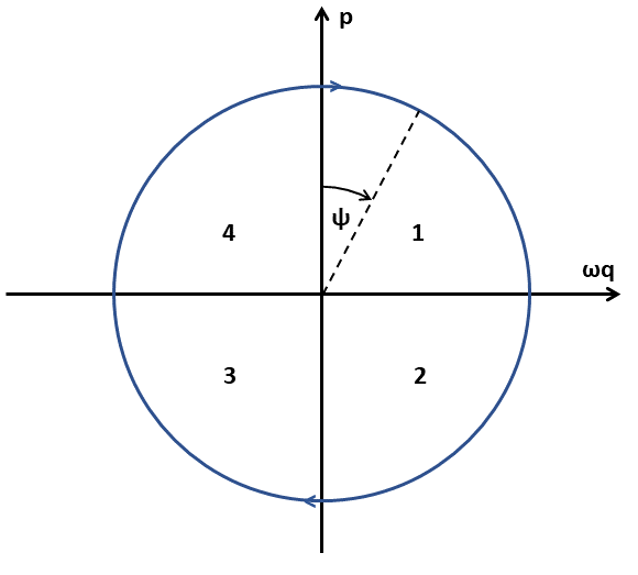
Figure 1: The angle $\psi$. We order the quadrants clockwise, i.e. in the direction of the motion.

4 Solving Hamilton equations for action-angle variables

4.1 Reduction to the Hamilton equation for the angle variable

We recall that the transformation $(q,p)\mapsto({\cal I},\psi)$ to the action, angle variables defined by

$${\cal I}=\frac{H}{\omega}=\frac{p^{2}+\omega^{2}q^{2}}{2\omega},\qquad\qquad\psi\,=\,\arg\,(p,\omega q),$$ (34)

as well as its inverse $({\cal I},\psi)\mapsto(q,p)$ defined by (10), remain canonical also if $\omega$ - and therefore also $H$ and themselves - depend on time. Therefore the evolution of ${\cal I},\psi$ is still ruled by the Hamilton equations, but with the transformed Hamiltonian $K({\cal I},\psi,t)$

$$\dot{\psi}=\frac{\partial K}{\partial{\cal I}},\qquad\dot{\cal I}=-\frac{\partial K}{\partial\psi},\qquad\quad K=\left[\omega+\frac{\dot{\omega}}{2\omega}\sin(2\psi)\right]{\cal I}$$

that can be obtained itself from a generating function of the transformation. More explicitly these equations read (11). The reader may check also by a direct computation that (1) and (11) are equivalent. From (10) it follows that the sequence of special points $\{t_{h}\}_{h\in\mathbb{Z}}$ (in the sense of Proposition 1) of every solution $q(t)$ is characterized, up to a multiple of $2\pi$, by

$$\psi(t_{h})=h\frac{\pi}{2},\qquad h\in\mathbb{Z}.$$ (36)

The Cauchy problem (11a) with $\psi(t_{*})=\psi_{*}$ is equivalent to the Volterra-type integral equation

$$\begin{array}[]{l}\displaystyle\psi(t)=\varphi(t)+\int^{t}_{y_{*}}\!\!dz\>\left[\frac{\dot{\omega}}{2\omega}\sin\left(2\psi\right)\right]\!(z),\\[14.0pt] \displaystyle\mbox{where }\varphi(t):=\psi_{*}+\!\int^{t}_{y_{*}}\!\!dz\>\omega(z)=:\psi^{(0)}(t).\end{array}$$ (39)

Once this is solved, (11b) with initial condition ${\cal I}(t_{*})={\cal I}_{*}$ is solved by

$${\cal I}(t)={\cal I}_{*}\exp\left\{-\!\!\int^{t}_{t_{*}}\!\!dz\left[\frac{\dot{\omega}}{\omega}\cos(2\psi)\right]\!(z)\right\};$$ (40)

the time-dependence of $H,q,p$ is obtained expressing them in terms of $\psi,{\cal I},\omega$. If $|\zeta|\equiv|\dot{\omega}/\omega^{2}|\ll 1$ (slowly/slightly varying $\omega$) then the integral in (39) can be neglected, the variation of ${\cal I}$ over time intervals $[t_{*},t]$ containing many cycles can be approximated replacing $\cos(2\psi)$ by its mean $0$ over a cycle, whence [cf. (15)]

$$\psi(t)\simeq\varphi(t),\qquad{\cal I}(t)\simeq{\cal I}(t_{*}),\qquad H(t)\simeq H(t_{*})\>\omega(t)/\omega(t_{*}).$$ (41)

The same applies if $\dot{\omega}/\omega$ oscillates about zero much faster than $\varphi$; such oscillations almost wash out the integrals in (39), (40). Improved estimates of such integrals lead to the better approximations reported below.

Eq. (11) make sense in intervals where $\omega$ is continuously differentiable, or is so at least piecewise while keeping continuous and with a bounded derivative. If $\omega(t)$ is continuous in $]t_{1},t_{2}[$ except at some point $t_{d}$, then in general so are $\ddot{q}(t),\psi(t),{\cal I}(t),H(t)$,whereas $q(t),p(t),r(t),s(t)$ are continuous in the whole $]t_{1},t_{2}[$. Let

$$\omega_{\pm}\!:=\!\lim\limits_{t\to t_{d}^{\pm}}\omega(t),\qquad\psi_{\pm}\!:=\!\lim\limits_{t\to t_{d}^{\pm}}\psi(t),\qquad{\cal I}_{\pm}\!:=\!\lim\limits_{t\to t_{d}^{\pm}}{\cal I}(t);$$ (42)

note that by their definitions [cf. (34)] both $\psi_{+},\psi_{-}$ must belong to the same quadrant of the $(q,p)$ plane. The continuities of $r,q,p$ at the discontinuity point $t_{d}$ of $\omega(t)$ imply the matching relations

$$\frac{\tan\psi_{+}}{\omega_{+}}=\frac{\tan\psi_{-}}{\omega_{-}},\qquad{\cal I}_{+}={\cal I}_{-}\,\frac{\omega_{-}}{\omega_{+}}\,\frac{1+\left(\frac{\omega_{+}}{\omega_{-}}\tan\psi_{-}\right)^{2}}{1+\tan^{2}\psi_{-}}.$$ (43)

The second determines the ‘sudden’ change of ${\cal I}$ due to the ‘sudden’ change of $\omega$; this depends not only on $\omega_{\pm}$, but also on the value of $\psi_{-}$ (or, equivalently, $\psi_{+}$). If  $t_{d}=t_{h}$, $h\in\mathbb{Z}$, then $\psi$ remains continuous because  $\tan\psi(t_{h})\!=\!0,\pm\infty$,  while

$${\cal I}_{+}\omega_{+}={\cal I}_{-}\omega_{-}\quad\mbox{if $h$ even},\qquad\quad{\cal I}_{+}\omega_{-}={\cal I}_{-}\omega_{+}\quad\mbox{if $h$ odd.}$$

The maximum, minimum possible ratio ${\cal I}_{+}/{\cal I}_{-}$ are therefore the ratios $\omega_{+}/\omega_{-}$, $\omega_{-}/\omega_{+}$, in either order. In general $\psi(t)$ can be extended from  $]t_{1},t_{d}[$  (resp.  $]t_{d},t_{2}[$)  to the whole $]t_{1},t_{2}[$ solving (11a) with (43a) as initial (resp. final) conditions in the complementary part. ${\cal I}(t)$ can be extended from  $]t_{1},t_{d}[$  (resp.  $]t_{d},t_{2}[$)  to the whole $]t_{1},t_{2}[$ applying (40) with (43b) as initial (resp. final) conditions in the complementary part.

4.2 Sequence converging to the solution of (39)

We can reformulate (39) in every compact time interval  $K:=[a,b]\supset t_{*}$   as the fixed point equation  ${\cal T}\psi=\psi$,  where ${\cal T}$ is the linear map ${\cal T}:C(K{})\to C(K{})$ defined by

$$[{\cal T}u](t):=\displaystyle\varphi(t)+\int^{t}_{t_{*}}\!\!dz\>f[z,u(z)],\qquad f(t,u):=\frac{\dot{\omega}(t)}{2\omega(t)}\sin\left(2u\right).$$ (44)

By means of the fixed point theorem one can build sequences $\{\psi^{(h)}\}_{h\in\mathbb{N}_{0}}\subset C(K)$ converging to its unique solution $\psi$. A very convenient one starts with $\psi^{(0)}:=\varphi$ and continues with

$$\psi^{(h)}(t):=[{\cal T}^{h}\varphi](t)=\varphi(t)+\int^{t}_{t_{*}}\!\!dz\>\left[\frac{\dot{\omega}}{2\omega}\sin\left(2\psi^{(h-1)}\right)\right]\!(z).$$ (45)

The corresponding sequence $\{{\cal I}^{(h)}\}_{h\in\mathbb{N}_{0}}$ converging to ${\cal I}$ arises replacing $\psi\mapsto\psi^{(h-1)}$ in (40)

$${\cal I}^{(h)}(t):={\cal I}(t_{*})\exp\left\{-\!\!\int^{t}_{t_{*}}\!\!dz\left[\frac{\dot{\omega}}{\omega}\cos\left(2\psi^{(h-1)}\right)\right]\!(z)\right\},$$ (46)

and the ones of $H,q,p$ are obtained replacing $({\cal I},\psi)\mapsto({\cal I}^{(h)},\psi^{(h)})$ in (34), (10). The ‘errors’ of approximation are conveniently bounded via the total variation of $\log\omega(t)$ between $t_{*},t$

$$g(t):=\int^{t}_{t_{*}}\!\!dz\left|\frac{\dot{\omega}(z)}{\omega(z)}\right|.$$ (47)

This grows with $t$, and $g(t_{*})=0$. If $\omega(t)$ is monotone in $[t_{*},t]$ then $g(t)=|\log\frac{\omega(t)}{\omega(t_{*})}|$; otherwise $g$ is the sum of a term of this kind for each monotonicity interval contained in $[t_{*},t]$.

Proposition 3

If $\omega\in C^{1}(K)$, with $\omega>0$, then for all $h\in\mathbb{N}$

$$\begin{array}[]{l}2\left|\psi(t)-\psi^{(h)}(t)\right|\,\leq\,\displaystyle\frac{|g(t)|^{h+1}}{(h\!+\!1)!}\>,\\[10.0pt] \left|\log{\cal I}(t)-\log{\cal I}^{(h)}(t)\right|\,\leq\,\displaystyle\frac{|g(t)|^{h+1}}{(h\!+\!1)!}\>.\end{array}$$ (50)

Consequently,  $\psi^{(h)}\to\psi$,   ${\cal I}^{(h)}\to{\cal I}$   in the sup norm of $C(K{})$,  $\|u\|_{\infty}:=\sup_{t\in K{}}\left\{|u(t)|\right\}$.

Proof    We start by deriving the following inequalities: for all $\alpha,\delta\in\mathbb{R}$

$$\begin{array}[]{l}|\sin(\alpha\!+\!\delta)\!-\!\sin\alpha|\leq\sqrt{2\left(1\!-\!\cos\delta\right)}\leq|\delta|,\\[6.0pt] |\cos(\alpha\!+\!\delta)\!-\!\cos\alpha|\leq\sqrt{2\left(1\!-\!\cos\delta\right)}\leq|\delta|.\end{array}$$ (51)

We abbreviate $f(\alpha,\delta):=\sin(\alpha\!+\!\delta)\!-\!\sin\alpha=\sin\alpha(\cos\delta\!-\!1)\!+\!\cos\alpha\,\sin\delta$. For fixed $\delta$ the points $\alpha^{\prime}$ of maximum, minimum for $f$ fulfill

$$0=\frac{\partial f}{\partial\alpha}(\alpha^{\prime},\delta)=\cos(\alpha^{\prime}\!+\!\delta)\!-\!\cos\alpha^{\prime}=\cos\alpha^{\prime}(\cos\delta\!-\!1)\!-\!\sin\alpha^{\prime}\sin\delta\quad\Rightarrow\quad\tan\alpha^{\prime}=\frac{\cos\delta\!-\!1}{\sin\delta}$$

$$f(\alpha^{\prime},\delta)=\cos\alpha^{\prime}\left[(\cos\delta\!-\!1)\tan\alpha^{\prime}\!+\!\sin\delta\right]=\frac{\cos\alpha^{\prime}}{\sin\delta}\left[(\cos\delta\!-\!1)^{2}\!+\!\sin^{2}\delta\right]=2\cos\alpha^{\prime}\,\frac{1\!-\!\cos\delta}{\sin\delta}$$

$$\Rightarrow\quad\left|f(\alpha,\delta)\right|\leq\left|f(\alpha^{\prime},\delta)\right|=\frac{2}{\sqrt{1\!+\!\tan^{2}\alpha^{\prime}}}\,\frac{1\!-\!\cos\delta}{\left|\sin\delta\right|}=\frac{2\left(1\!-\!\cos\delta\right)}{\sqrt{\sin^{2}\delta\!+\!\left(1\!-\!\cos\delta\right)^{2}}}=\sqrt{2(1\!-\!\cos\delta)},$$

as claimed; the right inequality in (51a) follows from the left one and the one  $1\!-\!\cos\delta\leq\frac{\delta^{2}}{2}$  (obtained integrating  $\sin x\leq x$ over $[0,\delta]$). Inequalities (51b) follow via the shift $\alpha\mapsto\alpha\!+\!\pi/2$.

By the assumptions it is $\mu:=\max_{K}\big{|}\frac{\dot{\omega}}{\omega}\big{|}<\infty$ and $M:=\max_{K}\{|g(t)|\}=\max\{|g(a)|,g(b)\}<\infty$.  Now abbreviate  $\sigma^{(h+1)}(t):=\psi(t)-\psi^{(h)}(t)$.  Eq. (39) implies

$$2\sigma^{(1)}(t)=\int^{t}_{t_{*}}\!\!dz\left[\sin(2\psi)\frac{\dot{\omega}}{\omega}\right]\!(z),\qquad\quad 2\left|\sigma^{(1)}(t)\right|\leq\int^{t}_{t_{*}}\!\!dz\left|\frac{\dot{\omega}(z)}{\omega(z)}\right|=g(t)\quad\mbox{if }\>t\geq t_{*},$$ (52)

i.e. (50) for $h=0$. If (50) holds for $h\!=\!j\!-\!1\geq 0$ it does also for $h\!=\!j$, since by eq. (39), (45)

$$2\sigma^{(j+1)}(t) \!=\! \int^{t}_{t_{*}}\!\!dz\left\{\frac{\dot{\omega}}{\omega}\left[\sin\left(2\psi\right)-\sin\left(2\psi^{(j-1)}\right)\right]\right\}\!(z),$$ (53)

$$2\left|\sigma^{(j+1)}(t)\right| \!\leq\! \int^{t}_{t_{*}}\!\!dz\left\{\left|\frac{\dot{\omega}}{\omega}\right|\left|\sin\left(2\psi^{(j-1)}\!+\!2\sigma^{(j)}\right)-\sin\left(2\psi^{(j-1)}\right)\right|\right\}\!(z)\leq\int^{t}_{t_{*}}\!\!dz\left|\frac{\dot{\omega}}{\omega}\,2\sigma^{(j)}\right|\!(z)$$

$$\!\leq\! \int^{t}_{t_{*}}\!\!dz\,\left[\left|\frac{\dot{\omega}}{\omega}\right|\frac{g^{j}\!\!}{j!}\right]\!(z)=\int^{t}_{t_{*}}\!\!\frac{dz}{(j\!+\!1)!}\,\frac{d}{dz}g^{j+1}(z)=\frac{[g(t)]^{j+1}}{(j\!+\!1)!}\qquad\mbox{if }\>t\geq t_{*}.$$

Similarly, eq. (40), (46) imply $\log[{\cal I}(t)/{\cal I}^{(j)}(t)]\!=\!\int^{t}_{t_{*}}\!\!dz\left\{\frac{\dot{\omega}}{\omega}\left[\cos\!\left(2\psi^{(j-1)}\right)\!-\!\cos\!\left(2\psi\right)\right]\right\}$, whence

$$\left|\log\frac{{\cal I}(t)}{{\cal I}^{(j)}(t)}\right| \!\leq\! \int^{t}_{t_{*}}\!\!dz\left\{\left|\frac{\dot{\omega}}{\omega}\right|\left|\cos\left(2\psi^{(j-1)}\right)-\cos\left(2\psi^{(j-1)}\!+\!2\sigma^{(j)}\right)\right|\right\}\!(z)\leq\int^{t}_{t_{*}}\!\!dz\left|\frac{\dot{\omega}}{\omega}\,2\sigma^{(j)}\right|\!(z)$$

$$\!\leq\! \int^{t}_{t_{*}}\!\!dz\,\left[\left|\frac{\dot{\omega}}{\omega}\right|\frac{g^{j}\!\!}{(j)!}\right]\!(z)=\int^{t}_{t_{*}}\!\!\frac{dz}{(j\!+\!1)!}\,\frac{d}{dz}g^{j+1}(z)=\frac{[g(t)]^{j+1}}{(j\!+\!1)!}\qquad\mbox{if }\>t\geq t_{*},$$

as claimed. If $t<t_{*}$ the previous inequalities hold if we exchange the extremes of integration $t,t_{*}$, thus proving (50) also in this case. From $|g(t)|\leq M$ we find rhs(50)$\leq M^{h+1}/(h\!+\!1)!$, which goes to zero as $h\!\to\!\infty$; this proves the mentioned convergences  $\psi^{(h)}\!\to\!\psi$, ${\cal I}^{(h)}\!\to\!{\cal I}$. $\sqcap$$\sqcup$

Corollary 1

If $\omega\in C^{1}(\mathbb{R})$, with $\omega>0$, then  $\psi^{(h)}\to\psi$,   ${\cal I}^{(h)}\to{\cal I}$  pointwise in all of $\mathbb{R}$.

Remarks:

1. The rate of the convergence  $\psi^{(h)}\to\psi$  for large $|t\!-\!t_{*}|$ is tipically much better than what the bounds (50) suggest. This makes the approximating sequence $\{\psi^{(h)}\}_{h\in\mathbb{N}_{0}}$ very useful also for practical purposes and numerical computations. In fact, if $|\varphi(t)\!-\!\psi_{*}|\gg\pi$ then the integrand of (52a) changes sign many times in $[t,t_{*}]$, thus reducing the magnitude of the integral and leading to $2\left|\sigma^{(1)}(t)\right|\ll|g(t)|$, unless $\dot{\omega}/\omega$ oscillates in phase with $\sin(2\varphi)$ (resonance). In the latter case, one can show that  lhs $\ll$ rhs   in (50) holds at least for the following corrections (i.e. for $h>1$).

2. Since  $|g(t)|\leq\mu|t\!-\!t_{*}|$,  the bounds (50) hold also replacing the rhs by  $[\mu|t\!-\!t_{*}|]^{h}/h!$.

3. The standard application of the fixed point theorem (see the appendix) also leads to  $\|\psi\!-\!\psi^{(h)}\|_{\infty}\to 0$,  but via the class of pointwise bounds (parametrized by $\lambda>\mu/2$)

   $$\left|\psi^{(h)}(t)\!-\!\psi(t)\right|\><\>e^{\lambda|t-t_{*}|}\>\frac{\nu^{h}}{1\!-\!\nu}\>\left\|\varphi\!-\!\psi^{(1)}\right\|_{\lambda,{\scriptscriptstyle K}}$$ (54)

   where $\nu:=\frac{\mu}{2\lambda}\in]0,1[$, $\|u\|_{\lambda,{\scriptscriptstyle K}}:=\max_{t\in K{}}\left\{|e^{-\lambda|t-t_{*}|}u(t)|\right\}$; the infimum $\sigma_{h,K}$ of the rhs over $\lambda\!\!\in]\mu/2,\infty[$ gives the most stringent bound in the class. Nevertheless, (54) is less manageable and stringent than (50a): as $h\to\infty$ the latter goes faster to zero, also due to the factorial in the denominator.

4. Once $\varphi$ is computed, through it we can readily use the approximation

   $$\hat{q}(t):=\sqrt{\frac{2{\cal I}^{(1)}(t)}{\omega(t)}}\>\sin\psi^{(0)}(t)=\sqrt{\frac{2{\cal I}(t_{*})}{\omega(t)}}\exp\left\{-\!\!\int^{t}_{t_{*}}\!\!dz\left[\frac{\dot{\omega}}{2\omega}\cos\left(2\varphi\right)\right]\!(z)\right\}\>\sin\varphi(t),$$ (55)

   which is an intermediate one between the above defined ones $q^{(0)}$ and $q^{(1)}$.

In the $h$-th approximation the discontinuity relations (43) become

$$\frac{\tan\psi^{(h)}_{+}}{\omega_{+}}=\frac{\tan\psi^{(h)}_{-}}{\omega_{-}},\quad\frac{{\cal I}^{(h)}_{+}}{\omega_{+}}\sin^{2}\!\psi^{(h)}_{+}=\frac{{\cal I}^{(h)}_{-}}{\omega_{-}}\sin^{2}\!\psi^{(h)}_{-},\quad{\cal I}_{+}\omega_{+}\cos^{2}\!\psi^{(h)}_{+}={\cal I}_{-}\omega_{-}\cos^{2}\!\psi^{(h)}_{-}.$$ (56)

Consequently, $\psi^{(h)}(t)$ is given by (45) for $t\in]t_{*},t_{d}[$, while for $t\in]t_{d},t_{f}[$ it is given by

$$\psi^{(h)}(t)=\psi^{(h)}_{+}+\int^{t}_{t_{d}}\!\!dz\>\left[\omega+\frac{\dot{\omega}}{2\omega}\sin\left(2\psi^{h-1}\right)\right]\!(z).$$ (57)

From these formulae one can derive an upper bound for the ‘error’ $\sigma^{(h+1)}_{+}\!:=\!\psi_{+}-\psi^{(h)}_{+}$ from one for the ‘error’ $\sigma^{(h+1)}_{-}\!:=\!\psi_{-}-\psi^{(h)}_{-}$, and conversely.

5 Usefulness of our approach

5.1 Adiabatic invariance of ${\cal I}$

The action variable ${\cal I}=H/\omega$ of the harmonic oscillator is the simplest example of an adiabatic invariant in a Hamiltonian system, in the sense that it remains approximately constant for slowly varying $\omega$s, as heuristic arguments suggest. Fixed a function  $\tilde{\omega}(\tau)$  and a ‘slow time’ parameter $\varepsilon>0$, consider the family of equations (1) with  $\omega(t;\varepsilon)=\tilde{\omega}(\varepsilon t)$. At least two precise senses are ascribed to the property of ‘adiabatic invariance’ of ${\cal I}$:

1. For all $(q_{0},p_{0})\in\mathbb{R}\times\mathbb{R}^{+}$ and $T,\delta>0$ one can choose $\varepsilon>0$ so small that for all   $t\in[0,T/\varepsilon]$  the solution of (1) with initial conditions $\big{(}q(0;\varepsilon),\dot{q}(0;\varepsilon)\big{)}=(q_{0},p_{0})$ satisfies

   $$|{\cal I}(t;\varepsilon)-{\cal I}(0;\varepsilon)|<\delta.$$ (58)

   Namely, if we slow down the rate of variation of $\omega$ proportionally to $\varepsilon$ and simultaneously dilate the time interval proportionally to $1/\varepsilon$, so that the $\tau$-interval $[0,T]$ and thus the variation of $\omega$ in $[0,T/\varepsilon]$ don’t change, the corresponding variation of ${\cal I}$ vanishes with $\varepsilon$. As known (see e.g. [2]), a sufficient condition for this is $\tilde{\omega}\in C^{2}(\mathbb{R}^{+})$.

2. If $\tilde{\omega}\in C^{k+1}(\mathbb{R})$ ($k\!\in\!\mathbb{N}$) and $\frac{d^{h}\tilde{\omega}}{d\tau^{h}}\in L^{1}(\mathbb{R})$ for all $h=1,...,k\!+\!1$ (whence $\tilde{\omega}(\tau)$ has well-defined limits and vanishing derivatives as $\tau\!\to\!\pm\infty$), then every solution of (1) satisfies (see e.g. [17])

   $$|{\cal I}(\infty;\varepsilon)-{\cal I}(-\infty;\varepsilon)|=O(\varepsilon^{k});$$ (59)

   if $\frac{d\tilde{\omega}}{d\tau}\in{\cal S}(\mathbb{R})$, i.e. is a Schwarz function (in particular, with compact support), then (59) holds for all $k\in\mathbb{N}$, namely the lhs goes to zero with $\varepsilon$ faster than any power.

In the appendix we prove both the sufficient condition in 1. and the implications in 2. quite fast via our approach (an example of its usefulness).

In section 6 we briefly mention some applications where these properties are important.

5.2 Asymptotic expansion in the slow-time parameter $\varepsilon$

Similarly, from the sequence $\{\psi^{(h)}\}_{h\in\mathbb{N}_{0}}$ one can obtain the asymptotic expansion of $\psi,{\cal I}$ in the slow time parameter $\varepsilon$ introduced in section 5.1. One can iteratively show that

$$\sigma^{(k)}=O(\varepsilon^{k}),\qquad\chi^{(h)}:=\psi^{(h)}-\psi^{(h-1)}=O(\varepsilon^{h}),\qquad\quad h=1,...,k-1.$$ (60)

Therefore the decomposition of $\psi=\psi^{(k-1)}\!+\!\sigma^{(k)}$ into a sum of $\psi^{(0)}$ and subsequent corrections

$$\psi=\psi^{(0)}+\chi^{(1)}+...+\chi^{(k-1)}+\sigma^{(k)}$$ (61)

is automatically a decomposition into terms $O(1),O(\varepsilon),...,O(\varepsilon^{k})$. Replacing in (40) one obtains the expansion for ${\cal I}$ via the Taylor formula for the exponential. Integrating by parts one can iteratively extract from each integral $\chi^{(h)}=\int^{t}_{t_{*}}\!\!dz\left\{\frac{\dot{\omega}}{\omega}\!\left[\sin\!\left(2\psi^{(h-1)}\right)\!-\!\sin\!\left(2\psi^{(h-2)}\right)\right]\!\right\}\!(z)$ the leading contribution as a more explicit function times $\varepsilon^{h}$, putting the rest in the remainder. In particular, for $k=2$ we obtain (choosing $t_{*}=0$ and abbreviating $\psi_{0}=\psi(0)$, $\tilde{\zeta}:=\frac{1}{\tilde{\omega}^{2}}\frac{d\tilde{\omega}}{d\tau}$)

$$\psi(t)=\varphi(t)-\frac{\varepsilon}{4}\left\{\cos\big{[}2\varphi(t)\big{]}\,\tilde{\zeta}(\varepsilon t)-\cos(2\psi_{0})\,\tilde{\zeta}(0)\right\}\!+O(\varepsilon^{2}),$$ (62)

$${\cal I}(t)={\cal I}_{0}\left\{1-\frac{\varepsilon}{2}\left[\sin\big{[}2\varphi(t)\big{]}\,\tilde{\zeta}(\varepsilon t)-\sin(2\psi_{0})\,\tilde{\zeta}(0)\right]\right\}+O(\varepsilon^{2}).$$ (63)

5.3 Upper and lower bounds on the solutions

We can easily bound $\psi(t),{\cal I}(t),H(t),...$ in an interval $[t_{h},t_{h+1}]$ where $\omega(t)$ is monotone.

If either $\dot{\omega}\geq 0$ and $h$ is even, or $\dot{\omega}\leq 0$ and $h$ is odd, then  $\dot{\omega}\sin(2\psi)\geq 0$ and by eq (11) $0\leq\dot{\psi}\!-\!\omega\leq(-1)^{h}\dot{\omega}/2\omega$; integrating in $[t_{h},t]$ with the initial condition $\varphi(t_{h})=\psi(t_{h})$ we find

$$\varphi(t)\leq\psi(t)\leq\varphi(t)+(-1)^{h}\log\sqrt{\frac{\omega(t)}{\omega(t_{h})}}=:\varphi^{(1)}(t)$$ (64)

for all $t\in[t_{h},t_{h+1}]$. In particular, choosing $t=t_{h+1}$ we find

$$0\leq\frac{\pi}{2}-\int^{t_{h+1}}_{t_{h}}\!\!\!\!\!\!dz\>\omega(z)\leq(-1)^{h}\log\sqrt{\frac{\omega(t_{h+1})}{\omega(t_{h})}}$$ (65)

which implicitly yield bounds on the length  $t_{h+1}\!-\!t_{h}$  of the interval $[t_{h},t_{h+1}]$ that are more stringent than (29). Moreover, let $\bar{t}_{h}\in[t_{h},t_{h+1}]$ be defined by the condition $\varphi^{(1)}(\bar{t}_{h+1})=(h\!+\!1)\pi/2$. By (36), $\cos(2w)$ decreases, grows with $w\in[\psi(t_{h}),\psi(t_{h+1})]=\left[\frac{h\pi}{2},\frac{(h\!+\!1)\pi}{2}\right]$ if $h$ is even, odd respectively. This and (64) imply in either case

$$-\frac{\dot{\omega}}{\omega}\cos(2\varphi)\leq-\frac{\dot{\omega}}{\omega}\cos(2\psi)\leq-\frac{\dot{\omega}}{\omega}\cos\left(2\varphi^{(1)}\right),$$ (66)

which replaced in (40) give

$$\exp\left\{-\!\!\int^{t}_{t_{h}}\!\!dz\left[\frac{\dot{\omega}}{\omega}\cos(2\varphi)\right]\!(z)\right\}\leq\frac{{\cal I}(t)}{{\cal I}(t_{h})}\leq\exp\left\{-\!\!\int^{t}_{t_{h}}\!\!dz\left[\frac{\dot{\omega}}{\omega}\cos\left(2\varphi^{(1)}\right)\right]\!(z)\right\};$$ (67)

the left bounds in (66-67) hold for all $t\in[t_{h},t_{h+1}]$, while the right ones only for $t\in[t_{h},\bar{t}_{h+1}]$.

Similarly, if $\dot{\omega}\!\leq\!0$ and $h$ is even, or $\dot{\omega}\!\geq\!0$ and $h$ is odd, then  $\dot{\omega}\sin(2\psi)\!\leq\!0$ and by eq. (11) $(-1)^{h}\dot{\omega}/2\omega\leq\dot{\psi}\!-\!\omega\leq 0$; integrating in $[t_{h},t]$ with the initial condition $\varphi(t_{h})=\psi(t_{h})$ we find

$$\varphi^{(1)}(t):=\varphi(t)+(-1)^{h}\log\sqrt{\frac{\omega(t)}{\omega(t_{h})}}\leq\psi(t)\leq\varphi(t)$$ (68)

for all $t\in[t_{h},t_{h+1}]$. In particular, choosing $t=t_{h+1}$ we find

$$(-1)^{h}\log\sqrt{\frac{\omega(t_{h+1})}{\omega(t_{h})}}\leq\frac{\pi}{2}-\int^{t_{h+1}}_{t_{h}}\!\!\!\!\!\!dz\>\omega(z)\leq 0$$ (69)

which implicitly yield more stringent bounds on  $t_{h+1}\!-\!t_{h}$  than (29). Moreover, let $\bar{t}_{h+1}^{\prime}\in[t_{h},t_{h+1}]$ be defined by the condition $\varphi(\bar{t}_{h+1}^{\prime})=(h\!+\!1)\pi/2$. Eq. (68) implies in either case again (66) and (67); the only difference is that now the right bounds hold for all $t\in[t_{h},t_{h+1}]$, while the left ones only for $t\in[t_{h},\bar{t}_{h+1}^{\prime}]$.

From (10), (67) and (64) or (68) one can now easily derive bounds on $q,p$.

If $\omega(t)$ is monotone in a larger interval $[t_{h},t_{h+k}]$ one can obtain there upper and lower bounds for $\psi(t)\!-\!\psi(t_{h})$ and the ratio ${\cal I}(t)/{\cal I}(t_{h})$ by using (64), (67) recursively in adjacent intervals. From the previous formulae and (34), (10) one obtains corresponding bounds for $H(t),q(t),p(t)$. The derivative  $\dot{H}=\dot{\omega}\omega q^{2}=2\dot{\omega}{\cal I}\sin^{2}\psi$  of $H$ along the solutions of (1) has the same sign of $\dot{\omega}$; therefore $H(t)$ grows, decreases where $\omega(t)$ does.

One could obtain upper and lower bounds also applying Liapunov’s direct method to the family of Liapunov functions  $V(t,\bar{\omega}):=\dot{q}{}^{2}(t)+\bar{\omega}^{2}q^{2}(t)$  parametrized by a positive constant $\bar{\omega}$. In each candidate interval $]t_{h},t_{h+1}[$ one makes two choices of $\bar{\omega}$, so as to make the derivative  $\dot{V}=2\dot{q}q(\bar{\omega}^{2}\!-\!\omega^{2})$  of $V$ along a solution $q(t)$ once positive and the other negative. Thus one determines upper and lower bounds first for $V$, then also for $q,\dot{q}$. However, it turns out that these bounds are rather less stringent and manageable than the ones found above.

5.4 Parametric resonance, beats, damping

Let us apply the previous results to the Hill equation, i.e. (1) with a periodic $\omega$,  $\omega(t+T)=\omega(t)$.  We recall that, by Floquet theorem, the fundamental matrix solution (18) of $\dot{V}=AV$ fulfills

$$V(t+nT)=V(t)M^{n},\qquad M:=V(T)$$ (70)

for all $t\in[0,T]$ and $n\in\mathbb{N}$, so it suffices to determine $V$ in $\in[0,T]$. As $\det M=1$, the eigenvalues of the monodromy matrix $M$ are $\lambda_{\pm}=\mu\pm\sqrt{\mu^{2}\!-\!1}$, where $2\mu:=\mbox{Tr}(M)$, hence fulfill $\lambda_{+}\lambda_{-}=1$. Consequently the two eigenvalues must do one of the following: i) be complex conjugate and of modulus 1 if $|\mu|<1$; coincide if $|\mu|=1$; be both real one larger, and one smaller than 1, if $|\mu|>1$. The trivial solution of (1) is stable if $|\mu|<1$, unstable if $|\mu|>1$ (most initial conditions near the trivial one yield parametrically resonant solutions), see e.g. [2, 17]. In terms of the solutions $\psi_{a}$ of (11a) fulfilling $\psi_{1}(0)=\frac{\pi}{2}$, $\psi_{2}(0)=0$, we find

$$2\mu=e^{-\Psi_{1}(T)}\sin[\psi_{1}(T)]+e^{-\Psi_{2}(T)}\cos[\psi_{2}(T)],$$ (71)

where $\Psi_{a}(t):=\!\!\int^{t}_{0}\!\!dz\left[\frac{\dot{\omega}}{2\omega}\cos(2\psi_{a})\right]\!(z)$,  $a=1,2$. If $\omega$ depends on a parameter $\eta$ so that  $\dot{\omega}/\omega=O(\eta)$,  then at leading order in $\eta$ (i.e., up to corrections of order 1,2,4) we find

$$\psi_{2}(t)=\psi_{1}(t)\!-\!\frac{\pi}{2}=\bar{\omega}t,$$

$$\Psi_{2}(t)=-\Psi_{1}(t)=\chi(t)$$

$$\mu=\cos(\bar{\omega}T)\,\cosh\left[\chi(T)\right],$$ (72)

where the characteristic (i.e. average) angular frequency $\bar{\omega}$ and $\chi(t)$ are defined by

$$\bar{\omega}:=\frac{\varphi(T)}{T},\qquad\chi(t)\!:=\!\!\int^{t}_{0}\!dz\left[\frac{\dot{\omega}}{2\omega}\cos(2\bar{\omega}t)\right]\!(z).$$

Clearly $\chi(T)=O(\eta)$. We recover parametric resonance if the period $T$ of variation of $\omega$ is one half of the characteristic time $2\pi/\bar{\omega}$, or a multiple thereof, namely if for some $j\in\mathbb{N}$

$$\bar{\omega}=j\,\frac{\pi}{T},$$ (73)

because then $\cos(\bar{\omega}T)=\pm 1$, and $|\mu|\simeq\cosh\left[\chi(T)\right]>1$, unless $\chi(T)=0$. Evaluating (71) one can determine the region in parameter space $(\bar{\omega},\eta)$ in the vicinity of a special value (73) leading to stable or unstable solutions. At lowest order in the small parameters  $\eta$ and  $b:=\bar{\omega}T\!-\!j\pi$  this amounts to evaluating (72). It is $\cos(\bar{\omega}T)=(-1)^{j}\cos b$, so that  $2|\mu|-2=\left[\chi(T)\right]^{2}-b^{2}+O(\eta^{4},b^{4})$;  therefore for sufficiently small $\eta,b$ the trivial solution will be stable if $|\chi(T)|<|b|$, parametrically resonant (hence unstable) if $|\chi(T)|>|b|$.

As an illustration, we determine at leading order in $|\eta|<1$ the solutions of (11) and $\mu$ if

$$\omega(t)=\bar{\omega}\sqrt{1+\eta\sin(\alpha t)},$$ (74)

with some constant $\alpha,\bar{\omega}>0$; the corresponding (1) is the well-known Mathieu equation (which rules many different phenomena, e.g. the forced motion of a swing, the stability of ships, the behaviour of parametric amplifiers based on electronic [13] or superconducting devices [22], parametrically excited oscillations in microelectromechanical systems; see e.g. [33] and references therein), and

$$T=\frac{2\pi}{\alpha},\qquad\frac{\dot{\omega}}{\omega}=\frac{\eta\alpha\cos(\alpha t)}{2[1\!+\!\eta\sin(\alpha t)]}$$

Denoting $\psi(0)=\psi_{*}$, ${\cal I}(0)={\cal I}_{*}$, we find  $\psi(t)=\psi^{(0)}(t)\!+\!O(\eta)=\psi_{*}\!+\!\bar{\omega}t\!+\!O(\eta)$, whence

$$\left[\frac{\dot{\omega}}{\omega}\cos\left(2\psi\right)\right]\!(t) = \frac{\eta\alpha}{2}\cos(\alpha t)\cos(2\psi_{*}\!+\!2\bar{\omega}t)+O(\eta^{2})$$

$$= \frac{\eta\alpha}{4}\big{\{}\cos[2\psi_{*}\!+\!(2\bar{\omega}\!-\!\alpha)t]+\cos[2\psi_{*}\!+\!(2\bar{\omega}\!+\!\alpha)t]\big{\}}+O(\eta^{2})$$

Replacing in (40) we find up to $O(\eta^{2})$  $\log[{\cal I}_{*}/{\cal I}(t)]=2\chi(t)$,  with

$$\chi(t)=\left\{\!\!\begin{array}[]{ll}\displaystyle\frac{\eta}{4}\bar{\omega}\left\{\cos(2\psi_{*})\,t+\frac{\sin(2\psi_{*}\!+\!4\bar{\omega}t)-\sin(2\psi_{*})}{4\bar{\omega}}\right\}&\mbox{if }\alpha=2\bar{\omega},\\[12.0pt] \displaystyle\frac{\eta\alpha}{8}\left\{\!\frac{\sin[2\psi_{*}\!+\!(2\bar{\omega}\!-\!\alpha)t]}{2\bar{\omega}\!-\!\alpha}+\frac{\sin[2\psi_{*}\!+\!(2\bar{\omega}\!+\!\alpha)t]}{2\bar{\omega}\!+\!\alpha}-\frac{4\bar{\omega}\sin(2\psi_{*})}{4\bar{\omega}^{2}\!-\!\alpha^{2}}\!\right\}&\mbox{if }\alpha\neq 2\bar{\omega}.\end{array}\right.$$ (77)

This leads to the following long-time behaviour. If $\alpha=2\bar{\omega}$ we find  ${\cal I}(t)\sim\exp[\eta\bar{\omega}\cos(2\psi_{*})t/2]$,  which exponentially vanishes with $t$ if $\eta\cos(2\psi_{*})<0$ (damping) or diverges with $t$ if $\eta\cos(2\psi_{*})>0$ (parametric resonance), respectively. Otherwise $\log{\cal I}(t)$ is the superposition of two sinusoids. In particular, for $\alpha\simeq 2\bar{\omega}$ the behaviour of $\log{\cal I}(t)$ is a typical beat: $\log[{\cal I}(t)/{\cal I}(0)]$ oscillates approximately between $\pm|\eta|\alpha/4|2\bar{\omega}\!-\!\alpha|$ with a period $T=2\pi/(2\bar{\omega}\!-\!\alpha)$. In fig.s 2, 3 we have plotted (in a short interval starting from $t=0$) the exact fundamental solutions $v_{a}$ introduced in section 2 and the corresponding action variables ${\cal I}_{a}$ ($a=1,2$), as well as their lowest approximations [in the sense of (16), (55)] $\tilde{v}_{a},\tilde{\cal I}_{a}$, $\hat{v}_{a},\hat{\cal I}_{a}$ for a non-resonant and a resonant choice of the parameters $\eta,\alpha$. As evident, our approximations $\hat{v}_{a},\hat{\cal I}_{a}$ fit the exact solutions much better than the ones $\tilde{v}_{a},\tilde{\cal I}_{a}$.

$\chi(T)$ is obtained setting  $\psi_{*}=0$, $t=T$.  At leading order in $\eta$ we find

$$\chi(T)=\left\{\!\!\begin{array}[]{ll}\displaystyle\eta\,\frac{\pi}{4}&\mbox{if }\alpha=2\bar{\omega},\\[8.0pt] \displaystyle\frac{\eta\alpha\bar{\omega}}{2[4\bar{\omega}^{2}\!-\!\alpha^{2}]}\sin\left(\!\frac{4\pi\bar{\omega}}{\alpha}\!\right)&\mbox{if }\alpha\neq 2\bar{\omega}.\end{array}\right.$$ (80)

Near the resonance point $T=\pi/\bar{\omega}$, i.e. for small  $b=\bar{\omega}T\!-\!\pi\equiv\pi(2\bar{\omega}/\alpha\!-\!1)$,  we find  $\chi(T)=\eta[\pi/4\!+\!O(b)]$  at lowest order in $b,\eta$. Therefore near $(\bar{\omega},\eta)=(\alpha/2,0)$ the regions fulfilling the inequalities  $\pi|\eta|<4|b|$  and  $\pi|\eta|>4|b|$,  or equivalently

$$|\eta|<4\left|\frac{2\bar{\omega}}{\alpha}\!-\!1\right|\qquad\mbox{and}\qquad|\eta|>4\left|\frac{2\bar{\omega}}{\alpha}\!-\!1\right|,$$

are respectively inside the stability and instability region, as known (see e.g. [17]). Near the resonance points  $T=j\,\frac{\pi}{\bar{\omega}}$ ($j>1$)  one can determine the (in)stability regions by a more precise evaluation of (71), which is out of the scope of this work.

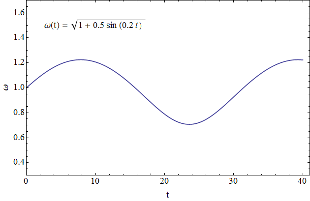
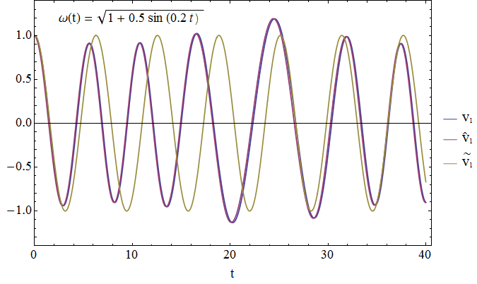
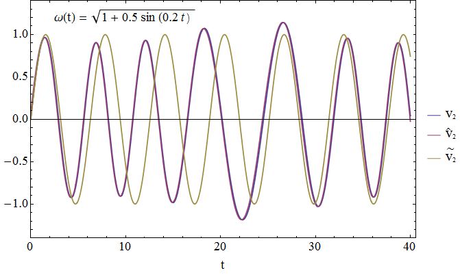
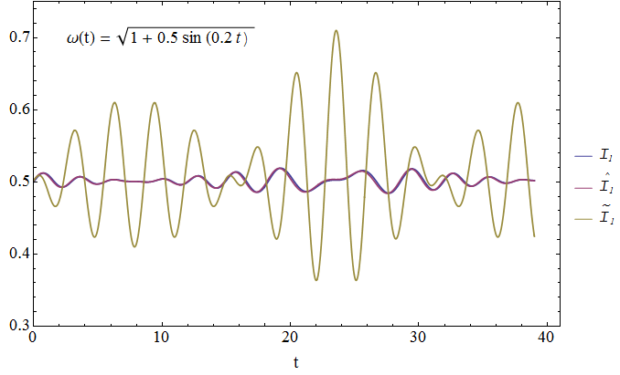
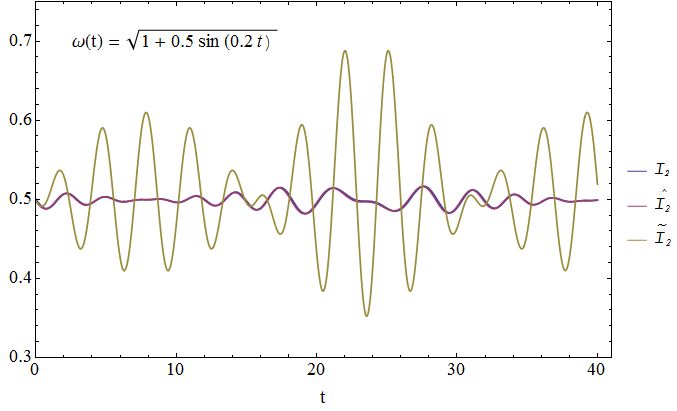
Figure 2: Mathieu equation with $\omega(t)=\bar{\omega}\sqrt{1+0.5\,\sin(0.2t)}$ (this is a non-resonant case). Up: graph of $\omega$; center: graphs of the two solutions $v_{a}$ ($a=1,2$) of (1) fulfilling $v_{1}(0)=\dot{v}_{2}(0)=1$, $v_{2}(0)=\dot{v}_{1}(0)=0$ (see section 2) and of their approximations $\hat{v}_{a},\tilde{v}_{a}$, with $a=1$ on the left, $a=2$ on the right; down: graphs of the corresponding action variable ${\cal I}_{a}$ and of their approximations $\hat{\cal I}_{a},\tilde{\cal I}_{a}$. As we can see, $\hat{v}_{a}\simeq v_{a}$, $\hat{\cal I}_{a}\simeq{\cal I}_{a}$, namely the approximation (55) is rather good, and much better than the one (16).

.       

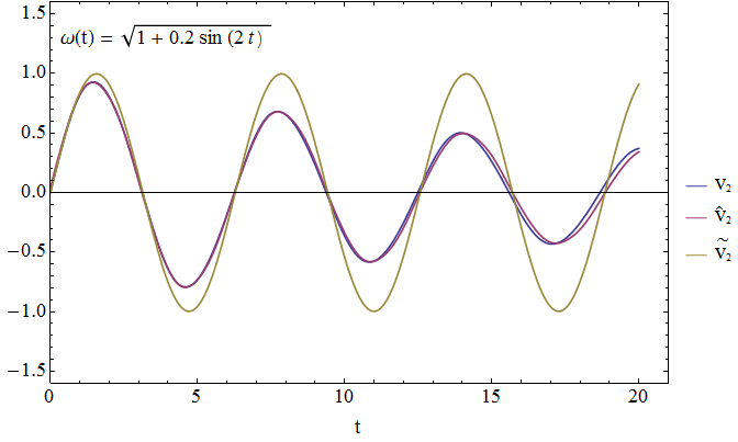
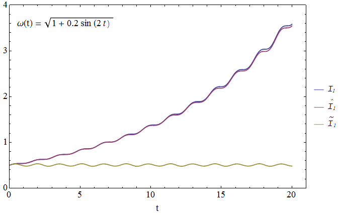
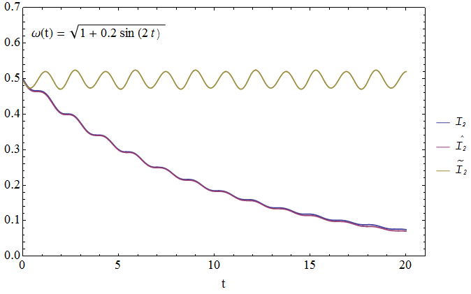
Figure 3: Mathieu equation with $\omega(t)=\bar{\omega}\sqrt{1+0.2\,\sin(2t)}$ (this is a resonant case). Up: graph of $\omega$; center: graphs of the two solutions $v_{a}$ ($a=1,2$) of (1) fulfilling $v_{1}(0)=\dot{v}_{2}(0)=1$, $v_{2}(0)=\dot{v}_{1}(0)=0$ (see section 2) and of their approximations $\hat{v}_{a},\tilde{v}_{a}$, with $a=1$ on the left, $a=2$ on the right; down: graphs of the corresponding action variable ${\cal I}_{a}$ and of their approximations $\hat{\cal I}_{a},\tilde{\cal I}_{a}$. Again, as we can see, $\hat{v}_{a}\simeq v_{a}$, $\hat{\cal I}_{a}\simeq{\cal I}_{a}$, namely the approximation (55) is rather good, and much better than the one (16).

6 Discussion and outlook

Solving equation (1) with $\omega(t)$ as general as possible, with high degrees of accuracy and/or for long times is paramount both for a deeper understanding of many natural phenomena and for developing sophisticated technological applications. For instance, the boundedness and stability of the solutions, or the knowledge of the tiny evolution of the adiabatic invariants under slowly varying $\omega$’s after millions or even billions of cycles $T=2\pi/\omega$, are crucial for many phenomena and problems in electrodynamics (in vacuum and plasmas) applied to geo- and astro-physics [24], accelerator physics [3, 32, 4], plasma confinement in nuclear fusion reactors [11]; in particular, rigorous mathematical results [16, 15, 23, 14, 34, 26] on the adiabatic invariance of ${\cal I}=H/\omega$ have allowed to dramatically increase the predictive power for these and other phenomena. A number of important classical and quantum control problems (like the stability of atomic clocks [31], the behaviour of parametric amplifiers based on electronic [13] or superconducting devices [22], or of parametrically excited oscillations in microelectromechanical systems [33]) are ruled by linear oscillator equations reducible to (1) (as sketched in section 2), where the interplay between time-dependent driving (parametric and/or external) and/or damping plays a crucial role [35]. In the quantum framework (1) arises e.g. as the evolution equation of the observable $q$ (a Hilbert space operator) in the Heisenberg picture (with imporant applications e.g. in quantum optics ), but also as the time-independent Schroedinger equation of a particle on $\mathbb{R}$ in a bounded potential $U(t)$ and with energy $E$, if we interpret $t$ as a space coordinate, $q(t)$ as the wave-function (which is again valued in numbers, but complex) and set $\omega^{2}\equiv 2m(E-U)/\hbar^{2}$; in particular, $E>0$ and a periodic $U(t)$, leading to periodic $\omega^{2}(t)$, determine (via Bloch theorem, an application of the Floquet one) the electronic bands structure of a crystal in solid state physics.

Here we have reduced (section 4) the integration of (1), or of more general linear systems (9) (section 2), to that of the first order ODE (11a), or equivalently the integral equation (39), in the globally defined unknown phase $\psi$ and adopted the iterative resolution procedure (45) to obtain sequences $\{\psi^{(h)}\}_{h\in\mathbb{N}_{0}}$ converging uniformly (and quite rapidly) to the solutions $\psi(t)$ in every compact interval where $\omega$ is differentiable; $\psi(t)$ can be extended beyond discontinuity points of $\omega(t)$, if any, by suitable matching conditions. As a preliminary step we have studied (section 3) the instants $t_{h}$ where $\psi$ is a multiple of $\pi/2$ (these are the interlacing zeroes of $q(t),\dot{q}(t)$). The applications sketched in the previous section 5 illustrate hopefully in a convincing way that our approach is economical and effective, and that its interplay with the existing wisdom and alternative approaches is rather promising for improving (both analitically and numerically) our knowledge of the solutions of (1) and of various delicate aspects of theirs. To that end, a comparison in particular with the Ermakov reformulation [7] seems appropriate now.

Looking for $q$ in the form of the product of an amplitude $\rho(t)$ and the sine of a phase $\theta(t)$,

$$q(t)=\rho(t)\sin[\theta(t)],$$ (81)

one easily finds that a sufficient condition for this to be a solution of (1) is that $\rho,\theta$ fulfill the ODEs

$$\rho\ddot{\theta}+2\dot{\rho}\dot{\theta}=0,\qquad\qquad\ddot{\rho}=-\omega^{2}\rho+\rho\dot{\theta}^{2},$$ (82)

which make the coefficients of $\sin\theta,\cos\theta$ vanish separately. By (82a), $\rho^{2}\dot{\theta}$ has zero derivative and hence is a constant $L$. Replacing $\rho^{2}\dot{\theta}\equiv L$ in (82b) we arrive at the Ermakov equation [7] in the unknown $\rho$

$$\ddot{\rho}=-\omega^{2}\rho+\frac{L^{2}}{\rho^{3}}.$$ (83)

Note that: i) the last term prevents $\rho$ to vanish anywhere; ii) the equation makes sense and yields solutions having continuous $\rho(t),\dot{\rho}(t)$ even if $\omega(t)$ is not. Given $L\neq 0$ and a particular solution $\rho(t)$ of (83), the corresponding $\theta(t)$ is found integrating $\dot{\theta}=L/\rho^{2}$. Actually the fulfillment of (82), or equivalently of (83) and $\theta(t)=\int^{t}\!\!d\tau L/\rho^{2}(\tau)$, is a sufficient condition for

$$q_{A,\alpha}(t):=A\,\rho(t)\sin[\theta(t)+\alpha],\qquad A,\alpha\in\mathbb{R}$$ (84)

to be the general solution of (1). In fact, fixed any conditions $\big{(}q(t_{*}),\dot{q}(t_{*})\big{)}=(q_{*},p_{*})$, if we set $\alpha=\left\{\cot^{-1}\!\left[(p_{*}\rho^{2}/q_{*}\!-\!\dot{\rho}\rho)/L\right]\!-\!\theta\right\}\!(t_{*})$, $A=q_{*}/[\rho\sin(\theta\!+\!\alpha)](t_{*})$ then $q_{A,\alpha}$ satisfies them. Conversely, assume $q,\rho$ solve (1), (83) with some constant $L\neq 0$. Then [7]

$$2I:=\left(q\dot{\rho}-\dot{q}\rho\right)^{2}+L^{2}\!\left(\frac{q}{\rho}\right)^{2},$$ (85)

is a constant because $\dot{I}=0$.   Of course, this exact invariant $I$ (usually dubbed after the names of Ermakov, Pinney, Courant, Snyder, Lewis, Riesenfeld, in various combinations) must not be confused with the adiabatic one ${\cal I}$. Only when $\omega=$const eq. (82) admits the constant solution $\rho=\sqrt{L/\omega}$, which, replaced in (85), gives $I=L{\cal I}$, namely coinciding $I,{\cal I}$, up to normalization. In general, the value of $I$ can be determined replacing in (85) the initial conditions fulfilled by $q,\rho$. In principle (85) allows to determine $\rho$ from $q$, and conversely, but not in closed form. A solution $\rho$ of (83) can be expressed explicitly [28] in terms of two independent solutions $u,v$ of (1) as follows:

$$\rho(t)=\sqrt{u^{2}(t)+\frac{L^{2}}{w^{2}}v^{2}(t)}\equiv\sqrt{q_{1}^{2}(t)+q_{2}^{2}(t)};$$ (86)

here $w=u\dot{v}-\dot{u}v=$const$\neq 0$ is the Wronskian of $u,v$, and in the last expression we have renamed $q_{1}:=u$, $q_{2}:=vL/w$. A nice way [6] to derive and interpret these results is to note that the vector ${\bm{\rho}}\equiv(q_{1},q_{2})$ satisfies again (1) regarded as a vector equation:

$$\ddot{\bm{\rho}}=-\omega^{2}(t){\bm{\rho}};$$ (87)

this is the equation of motion of a particle in a plane under the action of a time-dependent, but central elastic force (${\bm{\rho}}$ is its position vector with respect to the center $O$). Therefore the angular momentum $L:={\bm{\rho}}\times\dot{\bm{\rho}}=q_{1}\dot{q}_{2}\!-\!q_{2}\dot{q}_{1}$ (which coincides with the Wronskian of $q_{1},q_{2}$) is conserved. Decomposing ${\bm{\rho}}=(\rho\cos\theta,\rho\sin\theta)$, it is immediate to check that (82) amount to (87) written in the polar coordinates $\rho,\theta$,  and $L=\rho^{2}\dot{\theta}$. Replacing $q\mapsto q_{1}=\rho\cos\theta$ or $q\mapsto q_{2}=\rho\sin\theta$ in (85) one immediately finds that $2I=L^{2}$. If $q_{1},q_{2}$ are proportional then $L\!=\!0$, $\theta\!=$const, and the particle oscillates along a straight line passing through $O$; otherwise $L\neq 0$, and the particle goes around $O$. Finally, the invariant (85) is related also to the symmetries of the equation (1) (see [29, 35] and references therein). Probably it is worth underlining that in general $\rho\neq\sqrt{2{\cal I}/\omega}$, $\theta\neq\psi$ and, as already noted, ${\cal I}\neq I$, albeit (10a), (81) look similar, and both $\sqrt{2{\cal I}/\omega},\rho(t)$ - contrary to $q(t)$ - keep their sign, so that they can play the role of modulating amplitudes (envelopes) for the solutions of (1) resp. in (10), (81).

The exact invariant (85) is theoretically remarkable both in classical and quantum physics [however, in the latter case $q,p$ are operators, while $\rho$ remains a numerical solution of (83)]. For instance, in accelerator physics $I$ is a powerful constraint used to characterize the motion of a charged particle in alternating-gradient field configurations [3, 4]. In quantum mechanics the eigenvectors of the operator $I$ have time-independent eigenvalues, make up an orthonormal basis of the Hilbert space of states and may be normalized so as to be solutions of the Schroedinger equation; they can be built using ladder operators $a,a^{\dagger}$ as in the $\omega=$const case, and $I=a^{\dagger}a$ [18, 21, 20] (see e.g. also [25, 9]). However, the concrete use of $I$ is based on the knowledge of a solution of (83) for the specific problem at hand, but solving the second order ODE (83) is not easier than solving the one (1), except for special cases, and in general is more difficult than solving the first order ODE (11a). Therefore our iterative resolution method (45) could be used also for constructing solutions $\rho$ of (83) via (86).

Finding the most general conditions for the asymptotic stability of the trivial solution when there are no external forces and only the damping depends on time is also of interest [10].

Using our approach to determine the parametric resonance regions of (1) for specific classes of $\omega(t)$ (see e.g. [27]) is certainly also worth investigation.

7 Appendix

7.1 Proof of Proposition 1

For all $t_{*}\!\in\!\mathbb{R}$ it is $(q_{*},p_{*})\neq(0,0)$, because $q(t)$ is a nontrivial solution. If $q_{*}=0$ then respectively set $t_{0}:=t_{*}$ if $p_{*}>0$, $t_{2}:=t_{*}$ if $p_{*}<0$. If $q_{*}\neq 0$ then $r_{*}\in\mathbb{R}$; in the largest interval containing $t_{*}$ where $q(t)$ keeps its sign we find $-\dot{r}\geq\omega_{l}^{2}+r^{2}$, whence

$$\frac{-\dot{r}/\omega_{l}}{1+(r/\omega_{l})^{2}}=\frac{d}{dt}\cot^{-1}\!\left(\!\frac{r}{\omega_{l}}\!\right)\geq\omega_{l}\quad\Rightarrow\quad\cot^{-1}\!\left[\frac{r(t)}{\omega_{l}}\right]\geq\beta_{*}\!+\!\omega_{l}(t\!-\!t_{*})=:\varphi_{l}(t).$$ (88)

where $\beta_{*}\equiv\cot^{-1}\!\left(\frac{r_{*}}{\omega_{l}}\right)\!\in\,]0,\pi[$. Let $\bar{t}_{\pm}$ be defined by the conditions $\varphi_{l}(\bar{t}_{-})=0$, $\varphi_{l}(\bar{t}_{+})=\pi$; by construction $t_{*}\in]\bar{t}_{-},\bar{t}_{+}[$. The last inequality implies $r(t)/\omega_{l}\leq\cot\left[\varphi_{l}(t)\right]$; since the rhs goes to $-\infty$ as $t\uparrow\bar{t}_{+}$, there must exist a $t_{+}\!\in\,]t_{*},\bar{t}_{+}[$ such that $r(t)\to-\infty$ as $t\uparrow t_{+}$. If $p(t)>0$, $q(t)<0$ (resp. $p(t)<0$, $q(t)>0$) in a left neighbourhood of $t_{+}$ then the point $t_{0}:=t_{+}$ (resp. $t_{2}:=t_{+}$) has indeed the property mentioned in the claim.

In either case, now set $t_{*}\equiv t_{0}$ (resp. $t_{*}\equiv t_{2}$), $u\equiv\omega_{l}s$. In the largest interval $]t_{*},t_{+}^{\prime}[$ where $p(t)$ keeps its sign we find $\dot{s}\geq 1+u^{2}$, whence, integrating over $[t_{*},t]$,

$$\frac{\dot{u}}{1\!+\!u^{2}}=\frac{d}{dt}\tan^{-1}\!u\geq\omega_{l}\quad\Rightarrow\quad\tan^{-1}\!\left[u(t)\right]\geq\omega_{l}(t\!-\!t_{*})\quad\Rightarrow\quad\omega_{l}s(t)\geq\tan[\omega_{l}(t\!-\!t_{*})]$$ (89)

Since the rhs diverges as $t\uparrow t_{*}\!+\!\pi/2\omega_{l}$, it must be $t_{+}^{\prime}\!\in\,]t_{*},t_{*}\!+\!\pi/2\omega_{l}[$ and $s(t)\to+\infty$ as $t\uparrow t_{+}^{\prime}$; the point $t_{1}:=t_{+}^{\prime}$ (resp. $t_{3}:=t_{+}^{\prime}$) has indeed the property mentioned in the claim.

Setting $t_{*}=t_{1}$ (resp. $t_{*}=t_{3}$) and using again (88), with $\beta_{*}=\pi/2$, we prove the existence of $t_{2}$ (resp. $t_{4}$); setting $t_{*}=t_{2}$ (resp. $t_{*}=t_{4}$) and using again (89) we prove the existence of $t_{3}$ (resp. $t_{5}$); and so on. Replacing $t\mapsto-t$ in the equation and using the previous results one iteratively proves the existence of the $t_{h}$ for $h\!\in\!\mathbb{Z}$ going to $-\infty$.

Finally, if $\omega(t)\geq\bar{\omega}_{l}>0$ for all $t\in J\subset\mathbb{R}$ the claim follows from the previous case after extending $\omega(t)$ so that $\omega(t)\geq\bar{\omega}_{l}$ for all $t\in\mathbb{R}$.

7.2 Proof of Proposition 2

Lemma 1

Let $q_{1},q_{2}$ be two independent solutions of (1) having initial data at $t_{*}$ in the same quadrant of the $(q,p)$ plane, and let $\hat{t}_{1}>t_{*}$, $\hat{t}_{2}>t_{*}$ be the points where $q_{1},q_{2}$ change quadrant, respectively. Then $\hat{t}_{1}<\hat{t}_{2}$ provided the initial data of both $q_{1},q_{2}$ at $t_{*}$ fulfill either  $\dot{q}_{1*}q_{2*}<\dot{q}_{2*}q_{1*}\leq 0$,  or  $0\leq\dot{q}_{1*}q_{2*}<\dot{q}_{2*}q_{1*}$.

Proof    The difference of (26a) for the corresponding ratios $r_{1}=\dot{q}_{1}/q_{1},r_{2}=\dot{q}_{2}/q_{2}$ yields $\dot{r}_{1}\!-\!\dot{r}_{2}=-(r_{1}\!+\!r_{2})(r_{1}\!-\!r_{2})$. If the initial data of $q_{1},q_{2}$ at $t_{*}$ fulfill $\dot{q}_{1*}q_{2*}<\dot{q}_{2*}q_{1*}\leq 0$ (so that they both belong either to the first or to the third quadrant), then $r_{1}(t_{*})<r_{2}(t_{*})\leq 0$, $\dot{r}_{1}\!-\!\dot{r}_{2}$ is negative at $t=t_{*}$, keeps negative for all $t\in[t_{*},t^{\prime\prime}[$, and so does $r_{1}\!-\!r_{2}$; here $t^{\prime\prime}\!\equiv\!\min\{\hat{t}_{1},\hat{t}_{2}\}$. Hence $r_{2}$ cannot diverge before $r_{1}$, i.e. $t^{\prime\prime}=\hat{t}_{1}\leq\hat{t}_{2}$. Dividing by $(r_{1}\!-\!r_{2})$ we find that

$$\frac{d}{dy}\log(r_{2}-r_{1})=-(r_{1}\!+\!r_{2})\stackrel{{\scriptstyle t\to\hat{t}_{1}}}{{-\!\!\!-\!\!\!\longrightarrow}}+\infty$$

and this excludes that $r_{2}$ diverges together with $r_{1}$, i.e. we find $\hat{t}_{1}<\hat{t}_{2}$, as claimed.

Similarly, the difference of (26b) for the ratios $s_{1}=q_{1}/\dot{q}_{1},s_{2}=q_{2}/\dot{q}_{2}$ yields $\dot{s}_{1}\!-\!\dot{s}_{2}=\omega^{2}(s_{1}\!+\!s_{2})(s_{1}\!-\!s_{2})$. If the initial data of $q_{1},q_{2}$ at $t_{*}$ fulfill $0\leq\dot{q}_{1*}q_{2*}<\dot{q}_{2*}q_{1*}$ (so that they both belong either to the second or to the fourth quadrant) then $s_{1}(t_{*})>s_{2}(t_{*})\geq 0$, whence, arguing as before, $\hat{t}_{1}<\hat{t}_{2}$. $\sqcap$$\sqcup$

To show that $t_{i}^{\prime}>t_{i}$ implies $t_{h}(t_{i}^{\prime})>t_{h}(t_{i})$ for all $h\in\mathbb{Z}$ we apply the lemma setting  $q_{1}(t)\!\equiv\!Q(t;t_{i},q_{i},p_{i})$, $q_{2}(t)\!\equiv\!Q(t;t_{i}^{\prime},q_{i},p_{i})$.

We first consider the case that $q_{i}\leq 0$, $\dot{q}_{i}>0$ (fourth quadrant). Let us denote by $t_{0}(t_{i})$ the smallest $t\geq t_{i}$ such that $q_{1}(t)=0$ and by $t_{0}(t_{i}^{\prime})$ the smallest $t\geq t_{i}^{\prime}$ such that $q_{2}(t)=0$. In particular, if $q_{i}=0$, then $t_{0}(t_{i})=t_{i}>t_{i}^{\prime}=t_{0}(t_{i}^{\prime})$. If $q_{i}<0$ and $t_{i}^{\prime}\geq t_{0}(t_{i})$, then a fortiori $t_{0}(t_{i}^{\prime})>t_{i}^{\prime}\geq t_{0}(t_{i})$;  if $q_{i}<0$ and $t_{i}^{\prime}\in]t_{i},t_{0}(t_{i})[$, setting $t_{*}\equiv t_{0}(t_{i})$, we find $0=\dot{q}_{2*}q_{1*}>\dot{q}_{1*}q_{2*}$ and, applying the previous lemma, $t_{0}(t_{i})=\hat{t}_{1}<\hat{t}_{2}=t_{0}(t_{i}^{\prime})$. Namely, in all cases we find $t_{0}(t_{i}^{\prime})>t_{0}(t_{i})$, as claimed.

If $t_{0}(t_{i}^{\prime})\geq t_{1}(t_{i})$ then a fortiori $t_{1}(t_{i}^{\prime})>t_{1}(t_{i})$;  if $t_{0}(t_{i}^{\prime})\in]t_{0}(t_{i}),t_{1}(t_{i})[$, then setting $t_{*}\equiv t_{0}(t_{i}^{\prime})$ we find $0=\dot{q}_{1*}q_{2*}<\dot{q}_{2*}q_{1*}$ and, by the previous lemma, $t_{1}(t_{i})=\hat{t}_{1}<\hat{t}_{2}=t_{1}(t_{i}^{\prime})$; namely, in both cases we find $t_{1}(t_{i}^{\prime})>t_{1}(t_{i})$, as claimed.

If $t_{1}(t_{i}^{\prime})\geq t_{2}(t_{i})$ then a fortiori $t_{2}(t_{i}^{\prime})>t_{2}(t_{i})$;  if $t_{1}(t_{i}^{\prime})\in]t_{1}(t_{i}),t_{2}(t_{i})[$, then setting $t_{*}\equiv t_{1}(t_{i}^{\prime})$ we find $\dot{q}_{1*}q_{2*}<\dot{q}_{2*}q_{1*}=0$ and, by the previous lemma, $t_{2}(t_{i})=\hat{t}_{1}<\hat{t}_{2}=t_{2}(t_{i}^{\prime})$; namely, in both cases we find $t_{2}(t_{i}^{\prime})>t_{2}(t_{i})$, as claimed.

If $t_{2}(t_{i}^{\prime})\geq t_{3}(t_{i})$, then a fortiori $t_{3}(t_{i}^{\prime})>t_{3}(t_{i})$;  if $t_{2}(t_{i}^{\prime})\in]t_{2}(t_{i}),t_{3}(t_{i})[$, then setting $t_{*}\equiv t_{2}(t_{i}^{\prime})$, we find again $\dot{q}_{2*}q_{1*}>\dot{q}_{1*}q_{2*}=0$ and, by the previous lemma, $t_{3}(t_{i})=\hat{t}_{1}<\hat{t}_{2}=t_{3}(t_{i}^{\prime})$; namely, in both cases we find $t_{3}(t_{i}^{\prime})>t_{3}(t_{i})$, as claimed. And so on, for all nonnegative $h$. The claim for negative $h$ follows after replacing $t\mapsto-t$.

In the case that $q_{i}>0$, $\dot{q}_{i}\geq 0$ (first quadrant) we denote by $t_{1}(t_{i})$ the smallest $t\geq t_{i}$ such that $\dot{q}_{1}(t)=0$ and by $t_{1}(t_{i}^{\prime})$ the smallest $t\geq t_{i}^{\prime}$ such that $\dot{q}_{2}(t)=0$. In particular, if $\dot{q}_{i}=0$, then $t_{1}(t_{i})=t_{i}>t_{i}^{\prime}=t_{1}(t_{i}^{\prime})$. If $\dot{q}_{i}>0$ and $t_{i}^{\prime}\geq t_{1}(t_{i})$, then a fortiori $t_{1}(t_{i}^{\prime})>t_{i}^{\prime}\geq t_{1}(t_{i})$;  if $\dot{q}_{i}>0$ and $t_{i}^{\prime}\in]t_{i},t_{1}(t_{i})[$, setting $t_{*}\equiv t_{1}(t_{i})$, we find $0=\dot{q}_{1*}q_{2*}<\dot{q}_{2*}q_{1*}$ and, applying the previous lemma, $t_{1}(t_{i})=\hat{t}_{1}<\hat{t}_{2}=t_{1}(t_{i}^{\prime})$. Namely, in all cases we find $t_{1}(t_{i}^{\prime})>t_{1}(t_{i})$, as claimed. The rest of the proof goes as above.

In the case that $q_{i}\geq 0$, $\dot{q}_{i}<0$ (second quadrant) we denote by $t_{2}(t_{i})$ the smallest $t\geq t_{i}$ such that $q_{1}(t)=0$ and by $t_{2}(t_{i}^{\prime})$ the smallest $t\geq t_{i}^{\prime}$ such that $q_{2}(t)=0$. In particular, if $q_{i}=0$, then $t_{2}(t_{i})=t_{i}>t_{i}^{\prime}=t_{2}(t_{i}^{\prime})$. If $q_{i}<0$ and $t_{i}^{\prime}\geq t_{2}(t_{i})$, then a fortiori $t_{2}(t_{i}^{\prime})>t_{i}^{\prime}\geq t_{2}(t_{i})$;  if $q_{i}<0$ and $t_{i}^{\prime}\in]t_{i},t_{2}(t_{i})[$, setting $t_{*}\equiv t_{2}(t_{i})$, we find $\dot{q}_{1*}q_{2*}<\dot{q}_{2*}q_{1*}=0$ and, applying the previous lemma, $t_{2}(t_{i})=\hat{t}_{1}<\hat{t}_{2}=t_{2}(t_{i}^{\prime})$. Namely, in all cases we find $t_{2}(t_{i}^{\prime})>t_{2}(t_{i})$, as claimed. The rest of the proof goes as above.

In the case that $q_{i}<0$, $\dot{q}_{i}\leq 0$ (third quadrant) we denote by $t_{3}(t_{i})$ the smallest $t\geq t_{i}$ such that $\dot{q}_{1}(t)=0$ and by $t_{3}(t_{i}^{\prime})$ the smallest $t\geq t_{i}^{\prime}$ such that $\dot{q}_{2}(t)=0$. In particular, if $\dot{q}_{i}=0$, then $t_{3}(t_{i})=t_{i}>t_{i}^{\prime}=t_{3}(t_{i}^{\prime})$. If $\dot{q}_{i}<0$ and $t_{i}^{\prime}\geq t_{3}(t_{i})$, then a fortiori $t_{3}(t_{i}^{\prime})>t_{i}^{\prime}\geq t_{3}(t_{i})$;  if $\dot{q}_{i}<0$ and $t_{i}^{\prime}\in]t_{i},t_{3}(t_{i})[$, setting $t_{*}\equiv t_{3}(t_{i})$, we find $\dot{q}_{2*}q_{1*}>\dot{q}_{1*}q_{2*}=0$ and, applying the previous lemma, $t_{3}(t_{i})=\hat{t}_{1}<\hat{t}_{2}=t_{3}(t_{i}^{\prime})$. Namely, in all cases we find $t_{3}(t_{i}^{\prime})>t_{3}(t_{i})$, as claimed. The rest of the proof goes as above.

7.3 Proof of the bounds (54)

First note that $f(t,u)$ is continuous in $t$ and uniformly Lipschitz continuous in $u$, since

$$|f(t,u_{1})-f(t,u_{2})|\leq\frac{\mu}{2}|u_{1}\!-\!u_{2}|,\qquad\mu:=\sup_{K}\Big{|}\frac{\dot{\omega}}{\omega}\Big{|}<\infty.$$ (90)

For all $\lambda\in\mathbb{R}^{+}$ $C(K{})$ is a Banach space w.r.t. the norm $\|\>\|_{\lambda,{\scriptscriptstyle K}}$, which is equivalent to the one $\|\>\|_{\infty}$.  Eq. (90) implies  $\left|f[t,u_{1}(t)]-f[t,u_{2}(t)]\right|e^{-\lambda|t-t_{*}|}\leq(\mu/2)\|u_{1}\!-\!u_{2}\|_{\lambda,{\scriptscriptstyle K}}$, whence

$$\qquad\qquad\|{\cal T}u_{1}\!-\!{\cal T}u_{2}\|_{\lambda,{\scriptscriptstyle K}}\><\>\frac{\mu}{2\lambda}\>\|u_{1}\!-\!u_{2}\|_{\lambda,{\scriptscriptstyle K}}$$

for all $u_{1},u_{2}\in C(K{})$. This follows from the inequalities

$$\big{|}[{\cal T}\!u_{1}\!-\!{\cal T}\!u_{2}](t)\big{|}e^{\lambda(t_{*}-t)}\leq\int^{t}_{t_{*}}\!\!dz\>\big{|}f[z,\!u_{1}\!(z)]\!-\!f[z,\!u_{2}\!(z)]\big{|}e^{\lambda(t_{*}-t)}$$

$$\leq\frac{\mu}{2}\|u_{1}\!-\!u_{2}\|_{\lambda,{\scriptscriptstyle K}}\!\!\int^{t}_{t_{*}}\!\!dz\>e^{\lambda(t_{*}-z)}<\frac{\mu}{2\lambda}\>\|u_{1}\!-\!u_{2}\|_{\lambda,{\scriptscriptstyle K}}$$

if $t>t_{*}$, and from the ones with $t,t_{*}$ exchanged if $t<t_{*}$. Hence ${\cal T}$ is a contraction of $C(K{})$ provided we choose $2\lambda\!>\!\mu$; the fixed point theorem can be applied. Eq. (54) follows from the byproduct of that theorem

$$\left\|\psi^{(h)}\!-\!\psi\right\|_{\lambda,{\scriptscriptstyle K}}\><\>\frac{\nu^{h}}{1\!-\!\nu}\>\left\|\varphi\!-\!\psi^{(1)}\right\|_{\lambda,{\scriptscriptstyle K}},\qquad\quad\mbox{where }\>\nu:=\frac{\mu}{2\lambda}\in]0,1[.$$ (91)

7.4 Proof of the adiabatic invariance properties (58), (59)

If we adopt $\tau=\varepsilon t$ as the ‘time’ variable eq. (11a) takes the form

$$\frac{d\psi}{d\tau}=\frac{\tilde{\omega}}{\varepsilon}+\frac{1}{2\tilde{\omega}}\frac{d\tilde{\omega}}{d\tau}\sin(2\psi).$$ (92)

The function  $\varphi(\tau):=\varphi_{0}\!+\!\int^{\tau}_{0}\!\!d\tau^{\prime}\,\tilde{\omega}(\tau^{\prime})$ is strictly growing (here $\varphi_{0}\!\equiv\!\psi(0)$); to shorten the proof we make the further change of independent variable $\tau\mapsto\varphi$. We denote a transformed function putting a hat above its symbol, abbreviate $\hat{u}^{\prime}(\varphi)\equiv d\hat{u}/d\varphi$ and more generally $\hat{u}^{[h]}\equiv d^{h}\hat{u}/d\varphi^{h}$. As $\varphi$ is dimensionless, not only $\hat{\zeta}=\hat{\omega}^{\prime}/\hat{\omega}$, but also all derivatives $\hat{\zeta}^{\prime},\hat{\zeta}^{\prime\prime},...$ are; moreover, $\hat{\omega}(\varphi)$ fulfills the same conditions as $\tilde{\omega}(\tau)$, namely

$$\begin{array}[]{ll}\sup\limits_{\tau\in[0,T]}\left|\frac{d^{j}\tilde{\omega}}{d\tau^{j}}\right|<\infty,\quad c_{h}:=\sup\limits_{\alpha\in[\psi_{0},\varphi(T)]}\left|\hat{\zeta}^{[h]}(\alpha)\right|<\infty,\quad j=0,1,2,\quad h=0,1,&\mbox{in case 1},\\[12.0pt] \sup\limits_{\tau\in\mathbb{R}}\!\left|\frac{d^{j}\tilde{\omega}}{d\tau^{j}}\right|<\infty,\quad\sup\limits_{\mathbb{R}}\!\left|\hat{\zeta}^{[h]}\right|<\infty,\quad\hat{\zeta}^{[h]}\!\in\!L^{1}\!(\mathbb{R}),\quad j\!=\!0,\!...,k\!+\!1,\>\>h\!=\!0,\!...,k&\mbox{in case 2}.\end{array}$$ (95)

Eq. (92), (40) take the form

$$\hat{\psi}^{\prime}=\frac{f}{\varepsilon},\qquad f:=1+\varepsilon\frac{\hat{\zeta}}{2}\sin(2\hat{\psi})$$ (96)

$$-\log\frac{\hat{{\cal I}}(\varphi)}{\hat{{\cal I}}(\varphi_{*})}=\!\!\int^{\varphi}_{\varphi_{*}}\!\!d\beta\left[\hat{\zeta}\,\cos\left(2\hat{\psi}\right)\right]\!(\beta);$$ (97)

If $\tilde{\omega}\in C^{k+1}(\mathbb{R})$ then $\hat{\zeta}\in C^{k}(\mathbb{R})$, and the integral at the rhs of (97) can be transformed integrating by parts $k$ times. The result can be extracted as the real part of

$$\int^{\varphi}_{\varphi_{*}}\!\!d\beta\left[\hat{\zeta}\,e^{i2\hat{\psi}}\right]\!(\beta) = \int^{\varphi}_{\varphi_{*}}\!\!d\beta\>\frac{\varepsilon\hat{\zeta}(\beta)}{i2f(\beta)}\frac{d}{d\beta}e^{i2\hat{\psi}(\beta)}$$ (98)

$$= \left[e^{i2\hat{\psi}}\>\frac{\varepsilon\hat{\zeta}}{i2f}\right]^{\beta=\varphi}_{\beta=\varphi_{*}}\!\!+\int^{\varphi}_{\varphi_{*}}\!\!d\beta\left[e^{i2\hat{\psi}}\>\frac{d}{d\beta}\!\left(\frac{i\varepsilon\hat{\zeta}}{2f}\right)\!\right]\!(\beta)=...$$

$$= \left\{e^{i2\hat{\psi}}\sum_{h=0}^{k-1}\left(\!\frac{i\varepsilon}{2f}\frac{d}{d\beta}\!\right)^{h}\!\frac{\varepsilon\hat{\zeta}}{i2f}\!\right\}^{\beta=\varphi}_{\beta=\varphi_{*}}\!\!+\varepsilon^{k}\int\limits^{\varphi}_{\varphi_{*}}\!\!d\beta\left[e^{i2\hat{\psi}}\left(\!\frac{d}{d\beta}\frac{i}{2f}\!\right)^{k}\!\!v\right]\!\!(\beta).$$

In particular, if $\tilde{\omega}\in C^{2}(\mathbb{R})$ then

$$-\log\frac{\hat{{\cal I}}(\varphi)}{\hat{{\cal I}}(\varphi_{0})} = \varepsilon\left[\sin(2\hat{\psi})\>\frac{\hat{\zeta}}{2f}\right]^{\varphi}_{\varphi_{0}}\!\!-\frac{\varepsilon}{2}\int^{\varphi}_{\varphi_{0}}\!\!\!d\beta\left[\sin(2\hat{\psi})\>\frac{d}{d\beta}\!\left(\!\frac{\hat{\zeta}}{f}\!\right)\!\right]\!(\beta)$$

$$= \varepsilon\left[\sin(2\hat{\psi})\>\frac{\hat{\zeta}}{2f}\right]^{\varphi}_{\varphi_{0}}\!\!-\frac{\varepsilon}{2}\int^{\varphi}_{\varphi_{0}}\!\!\!d\beta\left[\sin(2\hat{\psi})\left(\frac{\hat{\zeta}^{\prime}}{f^{2}}\!-\!\frac{\hat{\zeta}^{2}}{f}\cos(2\hat{\psi})\!\right)\!\right]\!(\beta),$$

whence, noting that   $f>1\!-\!\varepsilon c_{0}/2$,

$$\left|\log\frac{\hat{{\cal I}}(\varphi)}{\hat{{\cal I}}(\varphi_{0})}\right|\leq\varepsilon\frac{\hat{\zeta}(\varphi)\!+\!\hat{\zeta}(0)}{2}+\frac{\varepsilon}{2}\int^{\varphi}_{0}\!\!\!d\beta\left(\left|\frac{\hat{\zeta}^{\prime}}{f^{2}}\right|\!+\!\left|\frac{\hat{\zeta}^{2}}{f}\right|\right)\!(\beta)\leq\varepsilon\left\{c_{0}\!+\!\frac{\varphi\!-\!0}{2(1\!-\!\varepsilon\frac{c_{0}}{2})}\left[\frac{c_{1}}{1\!-\!\varepsilon\frac{c_{0}}{2}}\!+\!c_{0}^{2}\right]\right\},$$

or, using again the time as the independent variable,

$$\left|\log\frac{{\cal I}(t)}{{\cal I}(0)}\right|\leq\varepsilon\left\{c_{0}\!+\!\frac{T\omega_{\scriptscriptstyle u}}{2\!-\!\varepsilon c_{0}}\left[\frac{c_{1}}{1\!-\!\varepsilon\frac{c_{0}}{2}}\!+\!c_{0}^{2}\right]\!\right\}=:M(\varepsilon),\quad\Rightarrow\quad|{\cal I}(t)-{\cal I}(0)|<{\cal I}(0)\left[e^{M(\varepsilon)}\!-\!1\right].$$

Clearly $M(\varepsilon)\to 0$ as $\varepsilon\!\to\!0$. Since $0\!<\!x\!\leq\!1$ implies $e^{x}\!-\!1\!<\!2x$, choosing $\varepsilon$ so small that $M(\varepsilon)\!<\!\min\big{\{}1,\delta/2{\cal I}(0)\big{\}}$ it follows $e^{M(\varepsilon)}\!-\!1\!<\!2M(\varepsilon)\!<\!\delta/{\cal I}(0)$, and (58) is fulfilled, as claimed. In case 2, by (95b) the terms in (98) outside the integral go to zero in the limits $\varphi_{*}\!\to\!-\infty$, $\varphi\!\to\!\infty$ because $\hat{\zeta}$ does, while the integral itself is bounded, so that $\left|\log\frac{\hat{{\cal I}}(\infty;\varepsilon)}{\hat{{\cal I}}(-\infty;\varepsilon)}\right|<N\varepsilon^{k}$ for some constant $N>0$. Arguing as above we conclude the proof of (59).

References

• [1] K. Andrzejewski and S. Prencel, Niederer’s transformation, time-dependent oscillators and polarized gravitational waves, Class. Quantum Grav. 36 (2019), 155008
• [2] V. I. Arnold, Mathematical methods of classical mechanics, Springer-Verlag, 1978.
• [3] E.D. Courant, H.S. Snyder, Theory of the alternating-gradient synchrotron, Ann. Phys. 3, 1-48 (1958).
• [4] R. C. Davidson and H. Qin, Physics of Intense Charged Particle Beams in High Energy Accelerators, World Scientific, Singapore, 2001.
• [5] A. Einstein, Inst. Intern. Phys. Solvay, Rapports et discussions 1, 450 (1911).
• [6] C. J. Eliezer and A. Gray, A Note on the Time-Dependent Harmonic Oscillator, SIAM J. Appl. Math., Vol. 30 (1976), pp. 463-468
• [7] V. P. Ermakov, Second-order differential equations: conditions of complete integrability, Univ. Izv. Kiev, vol. 20, p. 1 (1880). Translated in English: Appl. Anal. Discrete Math. 2 (2008), 123–145; available online at http://pefmath.etf.bg.ac.yu
• [8] G. Fiore, et al., On the impact of short laser pulses on cold diluted plasmas, in preparation.
• [9] G. Fiore, L. Gouba, Class of invariants for the two-dimensional time-dependent Landau problem and harmonic oscillator in a magnetic field, J. Math. Phys. 52 (2011), 103509.
• [10] L. Hatvani, On the Damped Harmonic Oscillator with Time Dependent Damping Coefficient, J. Dyn. Diff. Equat . 30 (2018), 25-37.
• [11] R. D. Hazeltine, J. D. Meiss, Plasma Confinement, Dover Publications, 2013.
• [12] J. Henrard, The Adiabatic Invariant in Classical Mechanics. In Dynamics Reported, Vol. 2, Springer, Berlin, 1993, p. 117-235.
• [13] Howson, D. P., Smith, R. B., Parametric Amplifiers, McGraw-Hill, New York, 1970.
• [14] G. Knorr, G. D. Pfirsch, The variation of the adiabatic invariant of the harmonic oscillator, Z. Naturforschung 21, 688 (1966)
• [15] M. Kruskal, Asymptotic Theory of Hamiltonian and other Systems with all Solutions Nearly Periodic, J. Math. Phys. 3, 806 (1962).
• [16] R. M. Kulsrud, Adiabatic Invariant of the Harmonic Oscillator, Phys. Rev. 106, 205 (1957).
• [17] L. D. Landau, E. M. Lifshitz, Mechanics, Butterworth-Heineman, Oxford, 1996.
• [18] H. R. Lewis , Classical and quantum systems with time-dependent harmonic-oscillator-type Hamiltonians, Phys. Rev. Lett. 18 (1967), 510; Erratum, Phys. Rev. Lett. 18, 636 (1967).
• [19] H. R. Lewis, Motion of a Time-Dependent Harmonic Oscillator, and of a Charged Particle in a Class of Time-Dependent, Axially Symmetric Electromagnetic Fields Phys. Rev. 172 (1968), 1313.
• [20] H. R. Lewis, W. B. Riesenfeld, An Exact Quantum Theory of the Time-Dependent Harmonic Oscillator and of a Charged Particle in a Time-Dependent Electromagnetic Field, J. Math. Phys. 10 (1969), 1458.
• [21] H. R. Lewis, Class of Exact Invariants for Classical and Quantum Time-Dependent Harmonic Oscillators, J. Math. Phys. 9 (1968), 1976.
• [22] Likharev, K. K., Dynamics of Josephson Junctions and Circuits, Gordon & Breach Science, Philadelphia, 1986.
• [23] J. E. Littlewood, Lorentz’s Pendulum Problem, Ann. Phys. 21, 233-242 (1963); Adiabatic invariance IV: Note on a New Method for Lorentz’s Pendulum Problem, Ann. Phys. 29, 13-18 (1964).
• [24] M. S. Longair, High Energy Astrophysics, Cambridge University Press, 2010.
• [25] V. I. Man’ko, Introduction to quantum optics, AIP Conf. Proc. 365 (1996), 337.
• [26] R.E. Meyer, Adiabatic variation part I. Exponential property for the simple oscillator, Z. angew. Math. Phys. 24, 293 (1973); Adiabatic variation part II. Action change for the simple oscillator, Z. angew. Math. Phys. 24, 517 (1973).
• [27] P. Nesterov, Appearance of New Parametric Resonances in Time-Dependent Harmonic Oscillator, Results. Math. 64 (2013), 229-251.
• [28] E. Pinney, The nonlinear differential equation $t"+p(x)y+cy^{-3}=0$, Proc. Am. Math. Soc., vol. 1, p. 681 (1950).
• [29] H. Qin, R. C. Davidson, Symmetries and invariants of the oscillator and envelope equations with time-dependent frequency, Phys. Rev. ST Accel. Beams 9, 054001 (2006)
• [30] Robnik, M., Recent results on time-dependent Hamiltonian oscillators, Eur. Phys. J. Spec. Top. 225, 1087–1101 (2016). https://doi.org/10.1140/epjst/e2016-02656-1
• [31] G M Saxena, Bikash Ghosal, Rubidium Atomic Clock: The Workhorse Of Satellite Navigation, (World Scientific, 2020).
• [32] K. Takayama, Dynamical invariant for forced time-dependent harmonic oscillator, Phys. Lett. A 88, Issue 2, 22 February 1982, Pages 57-59; Exact study of adiabaticity, Phys. Rev. A 45, 2618 (1992).
• [33] Turner, K.L., Miller, S.A., Hartwell, P.G., MacDonald, N.C., Strogatz, S.H., Adams, S.G.: Five parametric resonances in a microelectromechanical system, Nature 396, 149-152 (1998)
• [34] W. Wasow, Adiabatic Invariance of a Simple Oscillator, SIAM J. Math. Anal., 4 (1973), 78-88.
• [35] L. Zhang, W. Zhang, Lie transformation method on quantum state evolution of a general time-dependent driven and damped parametric oscillator, Ann. Phys. 373, 424-455 (2016).