Causal Regularization
On the trade-off between in-sample risk and out-of-sample risk guarantees

Lucas Kania lucaskania@cmu.edu Carnegie Mellon University Ernst Wit ernst.jan.camiel.wit@usi.ch Universitá della Svizzera italiana

Abstract

In recent decades, several data analytic ways of dealing with causality have been introduced, such as propensity score matching, the PC algorithm and invariant causal prediction. Although originally hailed for their interpretational appeal, here we study the identification of causal-like models from in-sample data that provide out-of-sample risk guarantees when predicting a target variable from a set of covariates.

Whereas ordinary least squares provides the best in-sample risk with limited out-of-sample guarantees, causal models have the best out-of-sample guarantees by sacrificing in-sample risk performance. We introduce causal regularization, by defining a trade-off between these properties. As the regularization increases, causal regularization provides estimators whose risk is more stable at the cost of increasing their overall in-sample risk. The increased risk stability is shown to result in out-of-sample risk guarantees. We provide finite sample risk bounds for all models and prove the adequacy of cross-validation for attaining these bounds.

1 Introduction

In many settings, the goal is to obtain models from in-sample data that are highly predictive for out-of-sample data. Heterogeneous in-sample data is oftentimes detrimental to discovering models that do not overfit (Hernan and Robins, 2010). However, when the heterogeneity in the sample can be attributed to a covariate shift that does not affect the functional relationship between the target and the covariates, the invariance of that structure implies that the causal model provides predictions that are robust to other future covariate shifts. Hence, the functional causal model is an interesting inferential goal also from a purely predictive point of view.

If the source of the covariate shift is known, instrumental variables (Didelez et al., 2010; Imbens, 2014) can be constructed. Alternatively, if the sample can be split into sub-samples that isolate different instances of the covariate shift, the causal model provides invariant predictions regardless of the sub-sample. Under linearity and non-confounding assumptions, Peters et al. (2016) noted that regressing the target on its direct causes returns a model that is invariant to the covariate shift across the sub-samples. They proposed an algorithm that regresses the target and all possible subsets of covariates in each sub-sample and tests which regression returns the same model regardless of the sub-sample. Under several heterogeneity sources, the authors proved that the algorithm identifies the causal model. Unfortunately, their search algorithm suffers from a combinatorial explosion and does not allow for confounding.

Arjovsky et al. (2019) resolves some of these issues by approximating the search algorithm, which results in more restricted guarantees regarding the identification of the causal model under linearity (Rosenfeld et al., 2020). Rothenhäusler et al. (2019) avoids the combinatorial search by limiting the source of heterogeneity. They model the covariate shift as a system of structural equations (SEM) being shifted by an instrument. In that scenario, the covariance between the covariates and the residuals under the causal model remains invariant across datasets. Given access to two datasets with different shifts, the difference between these invariant covariances provides a moment condition that uniquely identifies the causal model as long as the covariate shifts affect enough variables in the SEM. Estimating the moment condition gives rise to the causal Dantzig estimator. If the solution is not unique, the authors proposed an $L_{1}$ penalty to select a sparse approximation of the causal model. Under some stringent assumptions on the regularization parameter, finite sample bounds can be obtained for the distance between the causal model and the regularized estimator, but no risk guarantees were given for it.

Rojas-Carulla et al. (2018) showed that the prediction invariance of the causal model implies that it minimizes the maximum risk over all possible covariate shifts. Rothenhäusler et al. (2021) generalized that notion under the assumption that the covariate shift originates from an instrumental variable. Their key result is that the out-of-sample risk depends on the correlation between the residuals and the instrument. The more uncorrelated they are, the stronger the out-of-sample risk guarantees under unseen covariate shifts, whereby the causal model provides the best guarantees. Assuming access to the instrumental variable that generates the covariate shift, the authors propose to build a regularized estimator, called anchor regression, that regulates the amount of correlation between the residuals and the instrumental variable. From that correlation, the out-of-sample guarantees and finite sample bounds of all regularized models follow. Ideally, a regularized model should be chosen based on subject matter knowledge about the maximum future shift of the data. If it is not known, cross-validation is recommended, albeit no proof was provided regarding its adequacy for the proposed loss. Follow-up work extended the method to noisy instrumental variables (Oberst et al., 2021) and discrete and censored outcomes (Kook et al., 2021).

In this work, we consider the multiple datasets setting used in Rothenhäusler et al. (2019), but one in which there is no access to instrumental variables. We propose causal regularization for obtaining estimators that progressively decrease the risk bound on shifted out-of-sample datasets, akin to anchor regression. Unlike it, the instrument can be unknown, and the estimators are identifiable even when the unknown instrument does not shift all covariates. We provide finite sample risk bounds for all regularized models and prove the adequacy of cross-validation and data splitting for attaining these bounds.

It is worth remarking that the search for models that provide out-of-sample guarantees as a consequence of in-sample invariance parallels the idea of algorithmic stability (Villa et al., 2013). The main difference is that the latter studies out-of-sample risk bounds under the assumption that the training and test data come from the same distribution. Algorithmic stability requires model stability (Devroye and Wagner, 1979). This means that under sample perturbation (usually by leaving one observation out) the algorithm returns models that are similar, in the sense that their predictions do not differ much on average. Kearns and Ron (1999) and Bousquet and Elisseeff (2002) relaxed the stringent requirement of model stability to the requirement of risk stability, i.e., an algorithm returns models that have similar risk given perturbed samples. The work of Peters et al. (2016) follows the model stability approach, where they look for a model that has similar predictions under perturbed sub-samples, while Rothenhäusler et al. (2021), when using a categorical instrument that indicates the sub-samples, looks for a model that provides similar risk across sub-samples. Although the connection with risk stability is not immediate from their results, our work makes the requirement explicit and helps to elucidate the relationship between the two sub-fields.

2 Structural equation model with shifts

In this paper, we assume that the data generating process is given by a system of linear structural equations (SEM) and that the covariate shift across different datasets is produced by an exogenous random variable.

Definition 1 (Structural equation model).

A $\operatorname{SEM}(\operatorname{B},\operatorname{A})$ is defined as the stochastic solution $(X,Y)$ of

$$\begin{bmatrix}Y\\ X\end{bmatrix}=\underbrace{\operatorname{B}}_{\begin{subarray}{c}\text{constant}\\ \text{structure}\end{subarray}}\cdot\ \begin{bmatrix}Y\\ X\end{bmatrix}\ +\ \underbrace{\epsilon}_{\text{noise}}\ +\underbrace{\begin{bmatrix}0\\ \operatorname{A}\end{bmatrix}}_{\begin{subarray}{c}\text{covariate}\\ \text{shift}\end{subarray}}\operatorname{\text{ s.t. }}\operatorname{B}\mathrel{\vbox{\hbox{\scriptsize.}\hbox{\scriptsize.}}}=\begin{bmatrix}0&\operatorname{\beta_{PA}}^{T}\\ \operatorname{\beta_{CH}}&\operatorname{B_{X}}\end{bmatrix}\operatorname{\text{ and }}\epsilon\mathrel{\vbox{\hbox{\scriptsize.}\hbox{\scriptsize.}}}=\begin{bmatrix}\epsilon_{Y}\\ \epsilon_{X}\end{bmatrix}$$ (1)

where $X,\epsilon_{X},\operatorname{A}\in\operatorname{\mathbb{R}^{p}}$ and $Y,\epsilon_{Y}\in\operatorname{\mathbb{R}}$ are random vectors and variables, respectively. The matrix $\operatorname{B_{X}}\in\operatorname{\mathbb{R}^{p\times p}}$ consists of the interactions among the covariates $X$, the vector $\operatorname{\beta_{PA}}\in\operatorname{\mathbb{R}^{p}}$ describes the causal effects of $X$ on the target $Y$, and the vector $\operatorname{\beta_{CH}}\in\operatorname{\mathbb{R}^{p}}$ are the downstream effects of $Y$ on $X$.

The noise is identically distributed irrespective of the shift, i.e., for all $\operatorname{A}$ we have $\epsilon\sim{L}(0,\Sigma)$, some distribution with zero first moment and a finite second moment. Additionally, the shift $\operatorname{A}$ is assumed to be uncorrelated with the noise, i.e., $\operatorname{\mathbb{C}}[\operatorname{A},\epsilon]=0$. Finally, $I-\operatorname{B}$ is required to be non-singular in order for $\operatorname{SEM}(\operatorname{B},\operatorname{A})$ to be uniquely defined.

Let $\operatorname{{A}}$ be the set of all distributions that have a finite second moment, then $\operatorname{SEM}(\operatorname{B})\mathrel{\vbox{\hbox{\scriptsize.}\hbox{\scriptsize.}}}=\cup_{\operatorname{\operatorname{\tilde{A}}\in\operatorname{{A}}}}\operatorname{SEM}(\operatorname{B},\operatorname{\tilde{A}})$ is the set of all the possible realizations of the SEM for a constant structure $\operatorname{B}$ with noise distributed as ${L}(0,\Sigma)$. As our focus is on providing risk guarantees when predicting $Y$ from $X$, the SEM definition does not allow for a target shift. This is known as the exclusion restriction in the potential outcomes framework (Rubin, 1974). This assumption cannot be easily relaxed since a direct target shift affects the identifiability of the SEM. Conversely, all proved results in this work can be generalized to the case where the shift and noise variables are correlated and have a constant covariance over all possible shifts, i.e., $\operatorname{\mathbb{C}}[\operatorname{A},\epsilon]=\operatorname{\mathbb{C}}[\operatorname{\tilde{A}},\epsilon]\ \forall\operatorname{A},\operatorname{\tilde{A}}\in\operatorname{{A}}$.

Since the target is never directly shifted and the noise is identically distributed regardless of the shifted distribution, the residuals under the causal model $\operatorname{\beta_{PA}}$ are identically distributed for any shift distribution, i.e., $\forall\operatorname{A}\in\operatorname{{A}}$

$$\operatorname{Y^{\operatorname{{A}}}}-\operatorname{\beta_{PA}}^{T}\operatorname{X^{\operatorname{{A}}}}\quad=\quad\epsilon_{Y}\sim{L}_{Y}(0,\sigma^{2})~{}~{}\mbox{ independent of }\operatorname{A}.$$ (2)

Denote the risk of the using the model $\beta$ for $(\operatorname{X^{\operatorname{{A}}}},\operatorname{Y^{\operatorname{{A}}}})\mathrel{\vbox{\hbox{\scriptsize.}\hbox{\scriptsize.}}}=\operatorname{SEM}(\operatorname{B},\operatorname{A})$ as

$$\operatorname{R_{\operatorname{{A}}}}(\beta)=\operatorname{\mathbb{E}}[(\operatorname{Y^{\operatorname{{A}}}}-\beta^{T}\operatorname{X^{\operatorname{{A}}}})^{2}]$$ (3)

then due to (2) the risk using the causal parameters $\operatorname{R_{\operatorname{{A}}}}(\operatorname{\beta_{PA}})$ is invariant over ${A}$. In other words, the risk of the causal model is invariant to all shifts $A\in{A}$. Other models do not have this property since for $\beta\not=\operatorname{\beta_{PA}}$, there exists always a sequence of shifts such that the risk under $\beta$ is arbitrarily bad, i.e., $\exists\{\operatorname{A_{k}}\}_{k=1}^{\infty}\operatorname{\text{ s.t. }}\lim_{k\to\infty}\operatorname{R_{A_{k}}}(\beta)=\infty$. Hence, if the causal model were able to be estimated from in-sample data, then under that model the out-of-sample risk would be constant, which would be the best possible guarantee for the out-of-sample risk.

3 Causal regularization

Studies with data from well-designed randomized interventions are able to extract causal parameters (Fısher, 1935). In this paper, we assume we have much more unstructured data. We consider the setting, in which data from two distributions are available, for example from two separate studies. In particular, we assume that data is available from the observational distribution, i.e. $(\operatorname{X^{\operatorname{{0}}}},\operatorname{Y^{\operatorname{{0}}}})=\operatorname{SEM}(\operatorname{B},0)$, and a shifted distribution, i.e. $(\operatorname{X^{\operatorname{{A}}}},\operatorname{Y^{\operatorname{{A}}}})=\operatorname{SEM}(\operatorname{B},\operatorname{A})\operatorname{\text{ s.t. }}\operatorname{A}\not\equiv 0$. There is no direct access to the instrumental variable, i.e., the intervention, that generated the covariate shift $\operatorname{A}$.

3.1 Causal Dantzig

Rothenhäusler et al. (2019) noted that as the noise and shift are uncorrelated, the correlation between the predictors and the residual distribution under the causal model is invariant, i.e., the covariance $\operatorname{\mathbb{C}}[X,Y-\operatorname{\beta_{PA}}^{T}X]$ is constant for all $(X,Y)\in\operatorname{SEM}(\operatorname{B})$. Consequently, the difference in this quantity for two arbitrary distributions in $\operatorname{SEM}(\operatorname{B})$ is zero. This insight characterizes the causal parameter $\operatorname{\beta_{PA}}$, i.e.,

$$\operatorname{G_{\Delta}}\operatorname{\beta_{PA}}-\operatorname{Z_{\Delta}}=0$$ (4)

where $\operatorname{G_{\Delta}}\mathrel{\vbox{\hbox{\scriptsize.}\hbox{\scriptsize.}}}=\operatorname{\mathbb{E}}[\operatorname{X^{\operatorname{{A}}}}\operatorname{X^{\operatorname{{A}}}}^{T}]-\operatorname{\mathbb{E}}[\operatorname{X^{\operatorname{{0}}}}\operatorname{X^{\operatorname{{0}}}}^{t}]$ captures the shift in the covariates, and $\operatorname{Z_{\Delta}}\mathrel{\vbox{\hbox{\scriptsize.}\hbox{\scriptsize.}}}=\operatorname{\mathbb{E}}[\operatorname{X^{\operatorname{{A}}}}\operatorname{Y^{\operatorname{{A}}}}]-\operatorname{\mathbb{E}}[\operatorname{X^{\operatorname{{0}}}}\operatorname{Y^{\operatorname{{0}}}}]$ captures the shift of the target due to the covariate shift. The causal Dantzig estimator (Rothenhäusler et al., 2019) is defined as the solution of

$$\operatorname{\beta_{CD}}\mathrel{\vbox{\hbox{\scriptsize.}\hbox{\scriptsize.}}}=\operatorname*{arg\,min}_{\beta\in\operatorname{\mathbb{R}^{p}}}\left\lVert\operatorname{G_{\Delta}}\beta-\operatorname{Z_{\Delta}}\right\rVert_{2}$$ (5)

It is identifiable and unique, if and only if $\operatorname{G_{\Delta}}$ is full-rank, which happens if and only if $\operatorname{\mathbb{C}}[\operatorname{A}]$ is full-rank (see proposition 3 in appendix A). In this case $\operatorname{\beta_{CD}}=\operatorname{G_{\Delta}}^{-1}\operatorname{Z_{\Delta}}=\operatorname{\beta_{PA}}$. The authors use the infinity norm instead of the $L_{2}$ norm but the solutions are equivalent insofar $\operatorname{G_{\Delta}}$ is not singular.

If random samples $(\operatorname{\mathbb{X}^{\operatorname{{0}}}},\operatorname{\mathbb{Y}^{\operatorname{{0}}}})\in\operatorname{\mathbb{R}}^{\operatorname{n_{\operatorname{{0}}}}\times(p+1)}$ and $(\operatorname{\mathbb{X}^{\operatorname{{A}}}},\operatorname{\mathbb{Y}^{\operatorname{{A}}}})\in\operatorname{\mathbb{R}}^{\operatorname{n_{\operatorname{{A}}}}\times(p+1)}$ from the observational and shifted distributions are available, then the plug-in causal Dantzig estimator can be defined as

$$\operatorname{\hat{\beta}_{CD}}\mathrel{\vbox{\hbox{\scriptsize.}\hbox{\scriptsize.}}}=\operatorname*{arg\,min}_{\beta\in\operatorname{\mathbb{R}^{p}}}\left\lVert\operatorname{\mathbb{G}_{\Delta}}\beta-\operatorname{\mathbb{Z}_{\Delta}}\right\rVert_{2}$$ (6)

where $\operatorname{\mathbb{G}_{\Delta}}=\operatorname{\mathbb{X}^{\operatorname{{A}}}}^{T}\operatorname{\mathbb{X}^{\operatorname{{A}}}}/\operatorname{n_{\operatorname{{A}}}}-\operatorname{\mathbb{X}^{\operatorname{{0}}}}\operatorname{\mathbb{X}^{\operatorname{{0}}}}/\operatorname{n_{\operatorname{{0}}}}$ and $\operatorname{\mathbb{Z}_{\Delta}}=\operatorname{\mathbb{X}^{\operatorname{{A}}}}^{T}\operatorname{\mathbb{Y}^{\operatorname{{A}}}}/\operatorname{n_{\operatorname{{A}}}}-\operatorname{\mathbb{X}^{\operatorname{{0}}}}^{T}\operatorname{\mathbb{Y}^{\operatorname{{0}}}}/\operatorname{n_{\operatorname{{0}}}}$ are the plug-in estimators of $\operatorname{G_{\Delta}}$ and $\operatorname{Z_{\Delta}}$. If $\operatorname{\mathbb{G}_{\Delta}}$ or $\operatorname{G_{\Delta}}$ are rank deficient, the authors add an $L_{1}$ penalty, but no out-of-sample risk guarantees are given for the regularized estimators.

3.2 Causal regularization with risk guarantees

The aim of this work is to define a regularized version of the causal Dantzig estimator that (1) does not require the existence of a shift variable with a full-rank second moment and (2) has explicit risk guarantees over certain subsets of out-of-sample distributions. In other words, given data from $\operatorname{SEM}(\operatorname{B},0)$ and $\operatorname{SEM}(\operatorname{B},\operatorname{A})$, we want explicit guarantees for our performance on $\operatorname{SEM}(\operatorname{B},\operatorname{\tilde{A}})$, where $\operatorname{\tilde{A}}$ is larger than $\operatorname{A}$, in some precise sense. Hence, we consider the out-of-sample risk over the set $C_{\gamma}$ of shifts $\operatorname{\tilde{A}}$ that are at most $\gamma$-times stronger than $\operatorname{A}$, introduced in Rothenhäusler et al. (2021).

Definition 2 (Set of $\gamma$-times stronger shifts).

For a fixed shift-distribution $\operatorname{A}\in\operatorname{{A}}$, let $C_{\gamma}$ be the set of shifts that are $\gamma$-times stronger than $\operatorname{A}$, i.e.,

$$C_{\gamma}\mathrel{\vbox{\hbox{\scriptsize.}\hbox{\scriptsize.}}}=\left\{\operatorname{\operatorname{\tilde{A}}\in\operatorname{{A}}}~{}\left|~{}\begin{cases}\operatorname{\mathbb{E}}[\operatorname{\tilde{A}}\operatorname{\tilde{A}}^{T}]\preceq\gamma\operatorname{\mathbb{E}}[\operatorname{A}\operatorname{A}^{T}]&\operatorname{\text{if }}\gamma\in\operatorname{[0,\infty)}\\ \operatorname{supp}(\operatorname{\tilde{A}})=\operatorname{supp}(\operatorname{A})&\operatorname{\text{if }}\gamma=\infty\end{cases}\right.\right\}$$ (7)

where $M\preceq N$ if $M-N$ is positive semi-definite.

It is possible to decompose the worst out-of-sample risk over shifts in $\operatorname{C_{1+\tau}}$ into a weighted sum of the pooled risk and the risk difference without requiring the second moment of the shift variables to be full-rank. This is formalized in the following lemma.

Lemma 1 (Worst risk decomposition).

$$\forall\beta\in\operatorname{\mathbb{R}^{p}}\quad\operatorname{\sup_{\operatorname{\tilde{A}}\in\operatorname{C_{1+\tau}}}}\operatorname{R_{\operatorname{{\tilde{A}}}}}(\beta)=\frac{1}{2}\operatorname{\operatorname{R_{+}}}(\beta)+\frac{1+2\tau}{2}\operatorname{R_{\Delta}}(\beta),$$ (8)

$$\operatorname{\text{ where }}\quad\operatorname{\operatorname{R_{+}}}(\beta) \mathrel{\vbox{\hbox{\scriptsize.}\hbox{\scriptsize.}}}=\operatorname{R_{\operatorname{{A}}}}(\beta)+\operatorname{R_{\operatorname{{0}}}}(\beta)\mbox{ is the pooled risk}$$ (9)

$$\operatorname{R_{\Delta}}(\beta) \mathrel{\vbox{\hbox{\scriptsize.}\hbox{\scriptsize.}}}=\operatorname{R_{\operatorname{{A}}}}(\beta)-\operatorname{R_{\operatorname{{0}}}}(\beta)\mbox{ is the risk difference}$$ (10)

The risk difference directly measures the risk stability of the model across distributions, and it is related to the covariance invariance exploited by the causal Dantzig in the following sense: the smaller the risk difference, the more uncorrelated the residuals are of the model with the covariate shift generated by $\operatorname{A}$. This worst risk decomposition motivates the definition of causal regularization.

Definition 3 (causal regularization).

For $\lambda\in\operatorname{[0,\infty)}$, the causal regularizer $\operatorname{\beta_{\lambda}}$ is defined as the minimizer of the worst risk over $C_{(1+\lambda)/2}$,

$$\operatorname{\beta_{\lambda}}\mathrel{\vbox{\hbox{\scriptsize.}\hbox{\scriptsize.}}}=\operatorname*{arg\,min}_{\beta\in\operatorname{\mathbb{R}^{p}}}\frac{1}{2}\operatorname{R_{+}}(\beta)+\frac{\lambda}{2}\operatorname{R_{\Delta}}(\beta)$$ (11)

By increasing $\lambda$, causal regularization increases the pooled risk and reduces its risk difference across distributions, thereby increasing its risk stability. It is easy to check with the help of lemma 1 that, by definition, $\beta_{1+2\tau}$ optimizes the worst risk over $C_{1+\tau}$ where $\tau\in\operatorname{[0,\infty)}$. Letting the set of shifts $\operatorname{C_{1+\tau}}$ increase in magnitude towards the limit set $\operatorname{C_{\infty}}$, we recover that the normalized worst risk is equal to the risk difference,

$$\forall\beta\in\operatorname{\mathbb{R}^{p}}\quad\lim_{\tau\to\infty}\frac{\operatorname{\sup_{\operatorname{\tilde{A}}\in\operatorname{C_{1+\tau}}}}\operatorname{R_{\operatorname{{\tilde{A}}}}}(\beta)}{\tau}=\operatorname{R_{\Delta}}(\beta)$$ (12)

which means that the pooled risk under $\operatorname{\beta_{\lambda}}$ increases and the normalized worst out-of-sample risk decreases as $\lambda$ increases. In other words, the set of shifts, $\operatorname{C_{1+\tau}}$, for which $\operatorname{\beta_{\lambda}}$ provides risk guarantees increases as $\lambda$ increases.

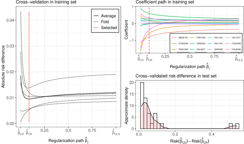
Figure 1: Causal regularization on gene knock-out experiments. (Left) $\hat{\beta}_{\text{CR}}$ denotes the model selected by 5-fold cross-validation. (Upper right) Coefficient path generated by causal regularization. (Lower right) Cross-validated risk difference on test set between the causal Dantzig and causal regularization. Observe that in all cases causal regularization achieves a smaller risk as evidence by $\text{Risk}(\hat{\beta}_{\text{CD}})-\text{Risk}(\hat{\beta}_{\text{CR}})$ being always positive.

Equation (12) also asserts that the regularizer $\operatorname{R_{\Delta}}(\beta)$ is non-negative for $\beta\in\operatorname{\mathbb{R}^{p}}$. This fact is elucidated by noting that it can be rewritten as a quadratic form centred at $\operatorname{\beta_{PA}}$, i.e.,

$$\operatorname{R_{\Delta}}(\beta)=(\beta-\operatorname{\beta_{PA}})^{T}\operatorname{G_{\Delta}}(\beta-\operatorname{\beta_{PA}})$$ (13)

as shown in proposition 4 in the appendix, which together with the positive semi-definiteness of $\operatorname{G_{\Delta}}$ imply the non-negativity of $\operatorname{R_{\Delta}}(\beta)$.

Based on the quadratic form, we can rewrite the regularizer in a way that clarifies the connection between causal Dantzig and causal regularization. The regularizer corresponds to the causal Dantzig objective multiplied by a pre-conditioner. Hence, by increasing the regularization, causal regularization approaches the causal Dantzig.

Proposition 1 (Convex regularizer).

$$\operatorname{R_{\Delta}}(\beta)=\operatorname{R_{||\cdot||}}(\beta)\operatorname{\text{ s.t. }}\operatorname{R_{||\cdot||}}(\beta)\mathrel{\vbox{\hbox{\scriptsize.}\hbox{\scriptsize.}}}=\left\lVert(G^{g/2}_{\Delta})^{T}(\operatorname{G_{\Delta}}\beta-\operatorname{Z_{\Delta}})\right\rVert_{2}^{2}$$ (14)

where $G^{g/2}_{\Delta}$ is the Moore–Penrose pseudoinverse of the square root of $\operatorname{G_{\Delta}}$, i.e., the matrix that satisfies $\operatorname{G_{\Delta}}=(G^{g/2}_{\Delta})^{T}G^{g/2}_{\Delta}$.

It follows that causal regularization interpolates between the causal Dantzig and ordinary least squares applied to both the observational and shifted distributions. The following corollary formalizes this notion.

Corollary 1 (Interpolation by causal regularization).

Let $\lambda\in\operatorname{[0,\infty)}$ and $\operatorname{G_{+}}\mathrel{\vbox{\hbox{\scriptsize.}\hbox{\scriptsize.}}}=\operatorname{\mathbb{E}}(\operatorname{X^{\operatorname{{A}}}}\operatorname{X^{\operatorname{{A}}}}^{T})+\operatorname{\mathbb{E}}(\operatorname{X^{\operatorname{{0}}}}\operatorname{X^{\operatorname{{0}}}}^{T})$, if $\operatorname{G_{+}}$ is non-singular, then

$$\beta_{\lambda}=\operatorname*{arg\,min}_{\beta\in\operatorname{\mathbb{R}^{p}}}\frac{1}{2}\operatorname{\operatorname{R_{+}}}(\beta)+\frac{\lambda}{2}\operatorname{R_{\Delta}}(\beta)=\operatorname*{arg\,min}_{\beta\in\operatorname{\mathbb{R}^{p}}}\left\lVert\operatorname{G_{\lambda}}\beta-\operatorname{Z_{\lambda}}\right\rVert_{2}^{2}=\operatorname{G_{\lambda}^{-1}}\operatorname{Z_{\lambda}}$$ (15)

where $\operatorname{G_{\lambda}}\mathrel{\vbox{\hbox{\scriptsize.}\hbox{\scriptsize.}}}=\operatorname{G_{+}}+\lambda\operatorname{G_{\Delta}}$ and $\operatorname{Z_{\lambda}}\mathrel{\vbox{\hbox{\scriptsize.}\hbox{\scriptsize.}}}=\operatorname{Z_{+}}+\lambda\operatorname{Z_{\Delta}}$. In particular, $\beta_{0}=\operatorname{G_{+}^{-1}}\operatorname{Z_{+}}$ is the population ordinary least squares. Additionally, if $\operatorname{G_{\Delta}}$ is non-singular, then $\beta_{\infty}\mathrel{\vbox{\hbox{\scriptsize.}\hbox{\scriptsize.}}}=\lim_{\lambda\to\infty}\beta_{\lambda}=\operatorname{G_{\Delta}^{-1}}\operatorname{Z_{\Delta}}$ is the causal Dantzig.

3.3 Empirical causal regularization

Consider the plugin estimates $\operatorname{\mathbb{Z}_{+}}\mathrel{\vbox{\hbox{\scriptsize.}\hbox{\scriptsize.}}}=\operatorname{\mathbb{X}^{\operatorname{{A}}}}^{T}\operatorname{\mathbb{Y}^{\operatorname{{A}}}}/\operatorname{n_{\operatorname{{A}}}}+\operatorname{\mathbb{X}^{\operatorname{{0}}}}^{T}\operatorname{\mathbb{Y}^{\operatorname{{0}}}}/\operatorname{n_{\operatorname{{0}}}}$, $\operatorname{\mathbb{G}_{+}}\mathrel{\vbox{\hbox{\scriptsize.}\hbox{\scriptsize.}}}=\operatorname{\mathbb{X}^{\operatorname{{A}}}}^{T}\operatorname{\mathbb{X}^{\operatorname{{A}}}}/\operatorname{n_{\operatorname{{A}}}}+\operatorname{\mathbb{X}^{\operatorname{{0}}}}^{T}\operatorname{\mathbb{X}^{\operatorname{{0}}}}/\operatorname{n_{\operatorname{{0}}}}$, $\operatorname{\mathbb{G}_{\lambda}}\mathrel{\vbox{\hbox{\scriptsize.}\hbox{\scriptsize.}}}=\operatorname{\mathbb{G}_{+}}+\lambda\operatorname{\operatorname{\mathbb{G}_{\Delta}}}$ and $\operatorname{\mathbb{Z}_{\lambda}}\mathrel{\vbox{\hbox{\scriptsize.}\hbox{\scriptsize.}}}=\operatorname{\mathbb{Z}_{+}}+\lambda\operatorname{\operatorname{\mathbb{Z}_{\Delta}}}$. Furthermore, let the empirical risk of $\beta$ on $(\operatorname{\mathbb{X}^{\operatorname{{A}}}},\operatorname{\mathbb{Y}^{\operatorname{{A}}}})$ be $\operatorname{\operatorname{\hat{R}_{\operatorname{{A}}}}}(\beta)=\left\lVert\operatorname{\mathbb{Y}^{\operatorname{{A}}}}-\operatorname{\mathbb{X}^{\operatorname{{A}}}}\beta\right\rVert_{2}^{2}/\operatorname{n_{\operatorname{{A}}}}$, and define the empirical pooled risk and risk difference as

$$\operatorname{\hat{R}_{+}}(\beta)\mathrel{\vbox{\hbox{\scriptsize.}\hbox{\scriptsize.}}}=\operatorname{\operatorname{\hat{R}_{\operatorname{{A}}}}}(\beta)+\operatorname{\hat{R}_{\operatorname{{0}}}}(\beta)\operatorname{\text{ and }}\operatorname{\hat{R}_{\Delta}}(\beta)\mathrel{\vbox{\hbox{\scriptsize.}\hbox{\scriptsize.}}}=\operatorname{\operatorname{\hat{R}_{\operatorname{{A}}}}}(\beta)-\operatorname{\hat{R}_{\operatorname{{0}}}}(\beta)$$ (16)

Every minimizer of $\frac{1}{2}\operatorname{\hat{R}_{+}}(\beta)+\frac{\lambda}{2}\operatorname{\hat{R}_{\Delta}}(\beta)$ satisfies the optimality condition $\operatorname{\mathbb{G}_{\lambda}}\beta=\operatorname{\mathbb{Z}_{\lambda}}$; hence, we define the causal regularization estimator $\operatorname{\hat{\beta}_{\lambda}}$ as the minimum norm least squares solution of the optimality condition, i.e., $\operatorname{\hat{\beta}_{\lambda}}=\operatorname{\mathbb{G}_{\lambda}^{g}}\operatorname{\mathbb{Z}_{\lambda}}$ where $\operatorname{\mathbb{G}_{\lambda}^{g}}$ denote the pseudoinverse of $\operatorname{\mathbb{G}_{\lambda}}$.

Definition 4 (Empirical causal regularization).

Given data from an observational and shifted environment, the empirical causal regularizer for $\lambda\in\operatorname{[0,\infty)}$ is defined as

$$\operatorname{\hat{\beta}_{\lambda}}\mathrel{\vbox{\hbox{\scriptsize.}\hbox{\scriptsize.}}}=\operatorname*{arg\,min}_{\beta\in M}\left\lVert\beta\right\rVert_{2}\operatorname{\text{ s.t. }}M\mathrel{\vbox{\hbox{\scriptsize.}\hbox{\scriptsize.}}}=\operatorname*{arg\,min}_{\beta\in\operatorname{\mathbb{R}^{p}}}\frac{1}{2}\operatorname{\hat{R}_{+}}(\beta)+\frac{\lambda}{2}\operatorname{\hat{R}_{\Delta}}(\beta)$$ (17)

or equivalently $\operatorname{\hat{\beta}_{\lambda}}=\operatorname{\mathbb{G}_{\lambda}^{g}}\operatorname{\mathbb{Z}_{\lambda}}$.

Its uniqueness is always guaranteed by the minimum norm condition (Planitz, 1979). Furthermore, if $\operatorname{\operatorname{\mathbb{G}_{\Delta}}}$ is full rank, the empirical causal regularization interpolates between the OLS estimator on all the data and the causal Dantzig estimator. Its consistency depends only on whether the population matrix $\operatorname{G_{+}}=\operatorname{\mathbb{E}}(\operatorname{X^{\operatorname{{A}}}}\operatorname{X^{\operatorname{{A}}}}^{T})+\operatorname{\mathbb{E}}(\operatorname{X^{\operatorname{{0}}}}\operatorname{X^{\operatorname{{0}}}}^{T})$ is full rank, while the consistency of $\operatorname{\hat{\beta}_{\infty}}$, the causal Dantzig estimator, depends on the non-singularity of $\operatorname{G_{\Delta}}$.

Proposition 2.

If $\operatorname{G_{+}}$ is positive definite, then $\operatorname{\hat{\beta}_{\lambda}}\operatorname{\overset{p}{\to}}\operatorname{\beta_{\lambda}}$ for $\lambda\in\operatorname{[0,\infty)}$

4 Finite sample bound for out-of-sample risk

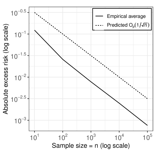
Figure 2: Absolute excess risk of $\operatorname{\beta_{PA}}$ as the sample size is increased. Note that both lines have approximately the same slope, indicating that the convergence rate matches the predicted one.

We derive a finite sample bound for the out-of-sample risk that can be used for any $\beta\in\operatorname{\mathbb{R}^{p}}$, and in particular for $\operatorname{\hat{\beta}_{\lambda}}$. The crux of the proof is to decompose the out-of-sample risk using lemma 1, and exploit the concentration of $\operatorname{\operatorname{\hat{R}_{\operatorname{{A}}}}}(\beta)$ and $\operatorname{\hat{R}_{\operatorname{{0}}}}(\beta)$ around $\operatorname{R_{\operatorname{{A}}}}(\beta)$ and $\operatorname{R_{\operatorname{{0}}}}(\beta)$, respectively (see proposition 5 in the appendix). The lemma assumes that covariates are normally distributed to avoid boundedness assumptions. The condition can be relaxed to sub-gaussian variables, and a distribution-free bound can be recovered by assuming bounded variables.

Lemma 2 (Finite sample bound for worst population risk).

If $\operatorname{\mathbb{X}^{\operatorname{{0}}}}$, $\operatorname{\mathbb{Y}^{\operatorname{{0}}}}$, $\operatorname{\mathbb{X}^{\operatorname{{A}}}}$ and $\operatorname{\mathbb{Y}^{\operatorname{{A}}}}$ are multivariate centred Gaussian variables

$$\forall\beta\in\operatorname{\mathbb{R}^{p}}:\quad\operatorname{\sup_{\operatorname{\tilde{A}}\in\operatorname{C_{1+\tau}}}}\operatorname{R_{\operatorname{{\tilde{A}}}}}(\beta)\leq\frac{1}{2}\operatorname{\hat{R}_{+}}(\beta)+\frac{1+2\tau}{2}\operatorname{\hat{R}_{\Delta}}(\beta)+\eta(\mathbf{n})$$ (18)

with probability exceeding $1-2e^{-q}$ for $q>0$, where

$$\eta(\mathbf{n}) \mathrel{\vbox{\hbox{\scriptsize.}\hbox{\scriptsize.}}}=(1+\tau)(\left\lVert\beta\right\rVert_{1}^{2}+1)\operatorname{\varphi}_{+}(p,\mathbf{n})$$ (19)

$$\operatorname{\varphi}_{+}(p,\mathbf{n}) \mathrel{\vbox{\hbox{\scriptsize.}\hbox{\scriptsize.}}}=\operatorname{\varphi}(p,\operatorname{n_{\operatorname{{A}}}})+\operatorname{\varphi}(p,\operatorname{n_{\operatorname{{0}}}})\quad\operatorname{\text{ and }}$$ (20)

$$\operatorname{\varphi}(p,\operatorname{n_{\operatorname{{U}}}}) \mathrel{\vbox{\hbox{\scriptsize.}\hbox{\scriptsize.}}}=\operatorname{\mathbb{V}}[\operatorname{Y^{\operatorname{{U}}}}]\left(\max_{1\leq k\leq p}\operatorname{\mathbb{V}}[\operatorname{X^{\operatorname{{U}}}_{k}}]\right)\left(\sqrt{\frac{4q+8\log(p)}{n_{\operatorname{{U}}}}}+\frac{4q+8\log(p)}{n_{\operatorname{{U}}}}\right)$$ (21)

Hence $\eta(\mathbf{n})=o_{p}\left(1/\sqrt{\min(\operatorname{n_{\operatorname{{A}}}},\operatorname{n_{\operatorname{{0}}}})}\right)$

We remark that due to the decomposition given in lemma 1, the inequality becomes an equality in the limit. Furthermore, $\hat{\beta}_{1+2\tau}$ can be motivated as the model that minimizes the first two terms of the RHS in equation (18) while controlling the norm $\left\lVert\hat{\beta}_{1+2\tau}\right\rVert_{2}$ which in turns controls $\eta(n)$.

Generally, the maximum future shift $\tau$ for which one wants guarantees is unknown. Thus, lemma 2 is mostly useful for controlling the normalized excess risk, i.e.,

$$\bar{\varphi}(\beta)\mathrel{\vbox{\hbox{\scriptsize.}\hbox{\scriptsize.}}}=\frac{\left(\frac{1}{2}\operatorname{\hat{R}_{+}}(\beta)+\frac{1+2\tau}{2}|\operatorname{\hat{R}_{\Delta}}(\beta)|\right)-\left(\operatorname{\sup_{\operatorname{\tilde{A}}\in\operatorname{C_{1+\tau}}}}\operatorname{R_{\operatorname{{\tilde{A}}}}}(\beta)\right)}{(1+\tau)(\left\lVert\beta\right\rVert_{1}^{2}+1)}\leq o_{p}\left(1/\sqrt{\min(\operatorname{n_{\operatorname{{A}}}},\operatorname{n_{\operatorname{{0}}}})}\right)$$ (22)

which is composed by the normalized excess pooled risk and the normalized excess risk difference

$$\bar{\varphi}(\beta)=\frac{1}{2}\ \left(\frac{\operatorname{\operatorname{\hat{R}_{+}}}(\beta)-\operatorname{\operatorname{R_{+}}}(\beta)}{(1+\tau)(\left\lVert\beta\right\rVert_{1}^{2}+1)}\right)\ +\ \frac{1+2\tau}{2}\ \left(\frac{|\operatorname{\hat{R}_{\Delta}}(\beta)|-\operatorname{R_{\Delta}}(\beta)}{(1+\tau)(\left\lVert\beta\right\rVert_{1}^{2}+1)}\right)$$ (23)

Figure 2 displays the empirical and predicted normalized excess risk as the sample sizes grow for the example shown in figure 4. The experiment details are deferred to section 7.1. Finally, the bound can be modified to provide guarantees for out-of-sample datasets.

Corollary 2 (Finite sample bound for worst sample risk).

If $\operatorname{\mathbb{X}^{\operatorname{{0}}}}$, $\operatorname{\mathbb{Y}^{\operatorname{{0}}}}$, $\operatorname{\mathbb{X}^{\operatorname{{A}}}}$, $\operatorname{\mathbb{Y}^{\operatorname{{A}}}}$, $\operatorname{\mathbb{X}^{\operatorname{{\tilde{A}}}}}$, and $\operatorname{\mathbb{Y}^{\operatorname{{\tilde{A}}}}}$ are multivariate centred Gaussian variables, and $\operatorname{{\tilde{A}}}\in C_{1+\tau}$

$$\forall\beta\in\operatorname{\mathbb{R}^{p}}:\quad\operatorname{\hat{R}_{\operatorname{{\tilde{A}}}}}(\beta)\leq\frac{1}{2}\operatorname{\hat{R}_{+}}(\beta)+\frac{1+2\tau}{2}|\operatorname{\hat{R}_{\Delta}}(\beta)|+\eta(\mathbf{n})$$ (24)

with probability exceeding $1-2e^{-q}$ for $q>0$, where

$$\eta(\mathbf{n})\mathrel{\vbox{\hbox{\scriptsize.}\hbox{\scriptsize.}}}=(\left\lVert\beta\right\rVert_{1}^{2}+1)\left((1+\tau)\operatorname{\varphi}_{+}(p,\operatorname{n_{\operatorname{{A}}}},\operatorname{n_{\operatorname{{0}}}})+\varphi(p,\operatorname{n_{\operatorname{{\tilde{A}}}}})\right)$$ (25)

The proof follows from upper-bounding $\operatorname{\hat{R}_{\operatorname{{\tilde{A}}}}}$ by $\operatorname{R_{\operatorname{{\tilde{A}}}}}$ via a concentration argument. Then, since $\operatorname{R_{\operatorname{{\tilde{A}}}}}(\beta)\leq\operatorname{\sup_{\operatorname{\tilde{A}}\in\operatorname{C_{1+\tau}}}}\operatorname{R_{\operatorname{{\tilde{A}}}}}(\beta)$, the corollary follows by applying lemma 2.

5 Model selection

So far, we have only considered out-of-sample risk evaluations for a fixed value of the regularization parameter $\lambda$. In this section, we consider selecting the regularization parameter based on resampling. The main idea is to design a model selection procedure that asymptotically chooses the same model as an oracle would with access to the unknown distributions $(\operatorname{X^{\operatorname{{0}}}},\operatorname{Y^{\operatorname{{0}}}})$ and $(\operatorname{X^{\operatorname{{A}}}},\operatorname{Y^{\operatorname{{A}}}})$.

Given a set of models $\{\hat{\beta}_{\lambda_{1}},\dots,\hat{\beta}_{\lambda_{K}}\}$ fitted on the in-sample data, a selector $\lambda$ is a choice of one of the models, i.e., $\lambda\in\Lambda\mathrel{\vbox{\hbox{\scriptsize.}\hbox{\scriptsize.}}}=\{\lambda_{1},\dots,\lambda_{K}\}$. Two selectors $\hat{\lambda}$ and $\lambda$ are asymptotically equivalent under some loss $\ell$, if their difference vanishes in probability asymptotically,

$$\ell(\hat{\lambda})-\ell(\lambda)\operatorname{\overset{p}{\to}}0.$$ (26)

Dudoit and van der Laan (2005) showed the asymptotic equivalence of the sample and population cross-validation selectors (defined for our situation in equations (34) and (33) below) under boundedness assumptions of both the target and covariates. Under further stringent conditions, they prove that the population cross-validation risk of the sample cross-validation selector is equivalent to the risk of the optimal selector, defined in equation (38) below. However, they did not prove that the optimal selector, which has access to models fitted with the full sample rather than a sub-sample, and the sample cross-validation selector are asymptotically equivalent. van der Vaart et al. (2006) relaxed the assumptions required for the asymptotic equivalence of the sample and population cross-validation selectors, replacing boundedness with pairs of Bernstein numbers. Nevertheless, they also did not prove their asymptotic equivalence with the optimal selector.

In this section, we prove, for a particular loss, that (i) the optimal selector, (ii) the sample cross-validation selector, and (iii) the population cross-validation selector are all asymptotically equivalent under normal covariates, i.e., without boundedness assumptions. The results follow from the concentration inequality described in lemma 2 (see proposition 5 in the appendix). The result can be generalized to sub-gaussian covariates. As before, distribution-free results can be recovered by assuming bounded covariates.

If the maximum future shift is unknown, one may want to choose a model that will perform well under arbitrarily strong shifts. Corollary 2 states that for arbitrary out-of-sample datasets, $\operatorname{\sup_{\operatorname{\tilde{A}}\in\operatorname{C_{1+\tau}}}}\operatorname{\hat{R}_{\operatorname{{\tilde{A}}}}}(\beta)$ concentrates around $\operatorname{\sup_{\operatorname{\tilde{A}}\in\operatorname{C_{1+\tau}}}}\operatorname{R_{\operatorname{{\tilde{A}}}}}(\beta)$. Thus, the bound given in lemma 2 can be used to perform model selection. Equation (12) tells us that the normalized worst out-of-sample risk is controlled by the population risk difference corresponding to the in-sample datasets, i.e., $\operatorname{R_{\Delta}}(\beta)$. Hence, minimizing $\operatorname{R_{\Delta}}(\beta)$ provides out-of-sample guarantees. Given that we only have access to random samples, performing sample-splitting or cross-validation on the absolute in-sample risk difference $|\operatorname{\hat{R}_{\Delta}}(\beta)|$ provides a useful surrogate loss. In the following, we show the validity of this idea.

We formally define data resampling in order to later recover the cross-validation and sample-splitting losses. Let $S^{\operatorname{{\tilde{A}}}}=(S^{\operatorname{{\tilde{A}}}}_{1},\dots,S^{\operatorname{{\tilde{A}}}}_{\operatorname{n_{\operatorname{{\tilde{A}}}}}})\in\{0,1\}^{n_{\operatorname{{\tilde{A}}}}}$ be a random variable that indicates if an observation from the dataset $(\operatorname{\mathbb{X}^{\operatorname{{\tilde{A}}}}},\operatorname{\mathbb{Y}^{\operatorname{{\tilde{A}}}}})$ is in the train or test set. That is, $S^{\operatorname{{\tilde{A}}}}_{i}=0$ means that $(x_{i}^{\operatorname{{\tilde{A}}}},y_{i}^{\operatorname{{\tilde{A}}}})$ is in the training set, while $S^{\operatorname{{\tilde{A}}}}_{i}=1$ indicates that it belongs to the test set. The distribution of $S^{\operatorname{{\tilde{A}}}}$ determines the methodology. For instance, if its distribution is a point mass at a unique binary string, i.e.,

$$\exists s\in\{0,1\}^{\operatorname{n_{\operatorname{{\tilde{A}}}}}}\operatorname{\text{ s.t. }}P(S^{\operatorname{{\tilde{A}}}}=s)=1$$ (27)

we recover sample-splitting. Alternatively, if there are $V$ binary strings among which the probability mass is homogeneously distributed, i.e.,

$$\exists s^{1},\dots,s^{V}\in\{0,1\}^{\operatorname{n_{\operatorname{{\tilde{A}}}}}}\operatorname{\text{ s.t. }}P(S^{\operatorname{{\tilde{A}}}}=s^{j})=1/V\operatorname{\text{ for }}j=1,\dots,V$$ (28)

where $\sum_{j=1}^{V}s_{i}^{j}=1\operatorname{\text{ and }}\sum_{i=1}^{\operatorname{n_{\operatorname{{\tilde{A}}}}}}s_{i}^{j}=n_{\operatorname{{\tilde{A}}}}/V$, we recover $V$-fold cross-validation. Note that $S^{\operatorname{{\tilde{A}}}}$ need not to be random but it must be stochastically independent from all observations, including those of other datasets. The notion can be formalized using extended conditional independence across the set ${S}$ of values that $S^{\operatorname{{\tilde{A}}}}$ can assume (Constantinou and Dawid, 2017), defined as

$$\forall s,\tilde{s}\in{S}\quad(\operatorname{\mathbb{X}^{\operatorname{{U}}}},\operatorname{\mathbb{Y}^{\operatorname{{U}}}})|S^{\operatorname{{\tilde{A}}}}=s\quad\sim\quad(\operatorname{\mathbb{X}^{\operatorname{{U}}}},\operatorname{\mathbb{Y}^{\operatorname{{U}}}})|S^{\operatorname{{\tilde{A}}}}=\tilde{s}\ \operatorname{\text{ for }}\operatorname{\tilde{A}},\operatorname{U}\in\{\operatorname{A},\operatorname{0}\}$$ (29)

The sub-empirical distributions $\mathbb{P}_{S,1}^{\operatorname{{\tilde{A}}}}$ and $\mathbb{P}_{S,0}^{\operatorname{{\tilde{A}}}}$ are defined by restricting the empirical distribution $\operatorname{\mathbb{P}_{\operatorname{n_{\operatorname{{\tilde{A}}}}}}^{\operatorname{{\tilde{A}}}}}$ to the corresponding set,

$$\operatorname{\mathbb{P}_{S^{\operatorname{{\tilde{A}}}},j}^{\operatorname{{\tilde{A}}}}}\mathrel{\vbox{\hbox{\scriptsize.}\hbox{\scriptsize.}}}=\frac{1}{\operatorname{n_{\operatorname{{\tilde{A}}}}(S^{\operatorname{{\tilde{A}}}},j)}}\sum_{i:\operatorname{S^{\operatorname{{\tilde{A}}}}_{i}}=j}^{\operatorname{n_{\operatorname{{\tilde{A}}}}(S^{\operatorname{{\tilde{A}}}},j)}}\delta_{i}^{\operatorname{{\tilde{A}}}}\operatorname{\text{ where }}\operatorname{n_{\operatorname{{\tilde{A}}}}(S^{\operatorname{{\tilde{A}}}},j)}\mathrel{\vbox{\hbox{\scriptsize.}\hbox{\scriptsize.}}}=\#\{1\leq i\leq\operatorname{n_{\operatorname{{\tilde{A}}}}}:\operatorname{S^{\operatorname{{\tilde{A}}}}_{i}}=j\}\operatorname{\text{ for }}j\in\{0,1\}\quad,$$ (30)

Let $S=(S^{\operatorname{{\tilde{A}}}},S^{\operatorname{{0}}})$ be the pair of indicators for each sample, and $(\operatorname{\mathbb{X}^{\operatorname{{\tilde{A}}}}_{S^{\operatorname{{\tilde{A}}}},j}},\operatorname{\mathbb{Y}^{\operatorname{{\tilde{A}}}}_{S^{\operatorname{{\tilde{A}}}},j}})\in\operatorname{\mathbb{R}}^{\operatorname{n_{\operatorname{{\tilde{A}}}}(S^{\operatorname{{\tilde{A}}}},j)}\times(p+1)}$ for $j\in{0,1}$ denote the design matrix and target vector corresponding to the previous sub-empirical distributions, then the in-sample risk on the test set is

$$\operatorname{\hat{R}_{\operatorname{{\tilde{A}}}}^{S,1}}(\beta)=\operatorname{\hat{R}_{\operatorname{{\tilde{A}}}}}(\beta,\operatorname{\mathbb{P}_{S^{\operatorname{{\tilde{A}}}},1}^{\operatorname{{\tilde{A}}}}})=\left\lVert\operatorname{\mathbb{Y}^{\operatorname{{\tilde{A}}}}_{S^{\operatorname{{\tilde{A}}}},1}}-\operatorname{\mathbb{X}^{\operatorname{{\tilde{A}}}}_{S^{\operatorname{{\tilde{A}}}},1}}\beta\right\rVert/\operatorname{n_{\operatorname{{\tilde{A}}}}(S^{\operatorname{{\tilde{A}}}},j)}$$ (31)

and the estimator fitted in the in-sample training set is given by equation (17), where $\operatorname{\mathbb{G}_{\lambda}}$ and $\operatorname{\mathbb{Z}_{\lambda}}$ are computed on the sub-sambples $\{(\operatorname{\mathbb{X}^{\operatorname{{\tilde{A}}}}_{S^{\operatorname{{\tilde{A}}}},0}},\operatorname{\mathbb{X}^{\operatorname{{\tilde{A}}}}_{S^{\operatorname{{\tilde{A}}}},0}})\}_{\operatorname{\operatorname{\tilde{A}}\in\{\operatorname{A},\operatorname{0}\}}}$ rather than the full samples $\{(\operatorname{\mathbb{X}^{\operatorname{{\tilde{A}}}}},\operatorname{\mathbb{Y}^{\operatorname{{\tilde{A}}}}})\}_{\operatorname{\operatorname{\tilde{A}}\in\{\operatorname{A},\operatorname{0}\}}}$

$$\operatorname{\hat{\beta}_{\lambda}^{S,0}}=\operatorname{\hat{\beta}_{\lambda}}(\operatorname{\mathbb{P}_{S^{\operatorname{{A}}},0}^{\operatorname{{A}}}},\operatorname{\mathbb{P}_{S^{\operatorname{{0}}},0}^{\operatorname{{0}}}})$$ (32)

We define the population and sample selectors as

$$\operatorname{\tilde{\lambda}_{S}} \mathrel{\vbox{\hbox{\scriptsize.}\hbox{\scriptsize.}}}=\operatorname*{arg\,min}_{\lambda\in\Lambda}\operatorname{\tilde{\theta}_{S}}(\lambda)\quad\operatorname{\text{ s.t. }}\quad \operatorname{\tilde{\theta}_{S}}(\lambda) \mathrel{\vbox{\hbox{\scriptsize.}\hbox{\scriptsize.}}}=\operatorname{\mathbb{E}}_{S}\operatorname{R_{\Delta}}(\operatorname{\hat{\beta}_{\lambda}^{S,0}})\qquad\text{Population selector}$$ (33)

$$\operatorname{\hat{\lambda}_{S}} \mathrel{\vbox{\hbox{\scriptsize.}\hbox{\scriptsize.}}}=\operatorname*{arg\,min}_{\lambda\in\Lambda}\operatorname{\hat{\theta}_{S}}(\lambda)\quad\operatorname{\text{ s.t. }}\quad \operatorname{\hat{\theta}_{S}}(\lambda) \mathrel{\vbox{\hbox{\scriptsize.}\hbox{\scriptsize.}}}=\operatorname{\mathbb{E}}_{S}|\operatorname{\hat{R}_{\Delta}^{S,1}}(\operatorname{\hat{\beta}_{\lambda}^{S,0}})|\qquad\text{Sample selector}$$ (34)

where the expectation is with respect to the sub-sampling distribution $S$ and where $\operatorname{\hat{R}_{\Delta}^{S,1}}(\beta)\mathrel{\vbox{\hbox{\scriptsize.}\hbox{\scriptsize.}}}=\operatorname{\hat{R}_{\operatorname{{A}}}^{S,1}}(\beta)-\operatorname{\hat{R}_{\operatorname{{0}}}^{S,1}}(\beta)$ is in-sample risk difference on the test set. It holds that the sample selector is asymptotically equivalent to the population selector

Lemma 3 (Asymptotic equivalence of sample and population selectors).

If $\operatorname{\mathbb{X}^{\operatorname{{0}}}}$, $\operatorname{\mathbb{Y}^{\operatorname{{0}}}}$, $\operatorname{\mathbb{X}^{\operatorname{{A}}}}$ and $\operatorname{\mathbb{Y}^{\operatorname{{A}}}}$ are multivariate centred Gaussian variables

$$|\operatorname{\tilde{\theta}_{S}}(\operatorname{\hat{\lambda}_{S}})-\operatorname{\tilde{\theta}_{S}}(\operatorname{\tilde{\lambda}_{S}})|\operatorname{\overset{p}{\to}}0$$ (35)

The result can be interpreted as follows. Define the optimal selector for a particular realization of $\{S^{\operatorname{{\tilde{A}}}}\}_{\operatorname{\operatorname{\tilde{A}}\in\{\operatorname{A},\operatorname{0}\}}}$, called the $S$-optimal selector, as

$$\operatorname{\tilde{\lambda}_{S,0}}=\operatorname*{arg\,min}_{\lambda\in\Lambda}\operatorname{\tilde{\theta}_{S,0}}(\lambda)\quad\operatorname{\text{ s.t. }}\quad\operatorname{\tilde{\theta}_{S,0}}(\lambda)\mathrel{\vbox{\hbox{\scriptsize.}\hbox{\scriptsize.}}}=\operatorname{R_{\Delta}}(\operatorname{\hat{\beta}_{\lambda}^{S,0}})\qquad\text{$S$-optimal selector}$$ (36)

The sample selector is asymptotically equivalent to the $S$-optimal selector for the average train-test split, as shown in the following corollary.

Corollary 3 (Asymptotic equivalence of sample and $S$-optimal selectors).

If $\operatorname{\mathbb{X}^{\operatorname{{0}}}}$, $\operatorname{\mathbb{Y}^{\operatorname{{0}}}}$, $\operatorname{\mathbb{X}^{\operatorname{{A}}}}$ and $\operatorname{\mathbb{Y}^{\operatorname{{A}}}}$ are multivariate centred Gaussian variables

$$|\operatorname{\mathbb{E}}_{S}[\operatorname{\tilde{\theta}_{S,0}}(\operatorname{\hat{\lambda}_{S}})-\operatorname{\tilde{\theta}_{S,0}}(\operatorname{\tilde{\lambda}_{S,0}})]|\operatorname{\overset{p}{\to}}0$$ (37)

Consequently, if the model selection methodology is such that the sub-empirical distributions $\{\mathbb{P}_{S,0}^{\operatorname{{\tilde{A}}}}\}_{\operatorname{\operatorname{\tilde{A}}\in\{\operatorname{A},\operatorname{0}\}}}$ converge in law to the empirical distributions $\{\mathbb{P}_{\operatorname{n_{\operatorname{{\tilde{A}}}}}}^{\operatorname{{\tilde{A}}}}\}_{\operatorname{\operatorname{\tilde{A}}\in\{\operatorname{A},\operatorname{0}\}}}$ as $\operatorname{n_{\operatorname{{A}}}}$ and $\operatorname{n_{\operatorname{{0}}}}$ grow to infinity, then $\operatorname{\hat{\beta}_{\lambda}^{S,0}}$ converges to $\operatorname{\hat{\beta}_{\lambda}}(\mathbb{P}_{\operatorname{n_{\operatorname{{A}}}}}^{\operatorname{{A}}},\mathbb{P}_{\operatorname{n_{\operatorname{{0}}}}}^{\operatorname{{0}}})$ due to the continuity of the estimator, and the sample selector is on average asymptotically equivalent to the optimal selector, defined as

$$\operatorname{\tilde{\lambda}}\mathrel{\vbox{\hbox{\scriptsize.}\hbox{\scriptsize.}}}=\operatorname*{arg\,min}_{\lambda\in\Lambda}\tilde{\theta}(\lambda)\quad\operatorname{\text{ s.t. }}\quad\tilde{\theta}(\lambda)\mathrel{\vbox{\hbox{\scriptsize.}\hbox{\scriptsize.}}}=\operatorname{R_{\Delta}}(\operatorname{\beta_{\lambda}}(\operatorname{\mathbb{P}_{\operatorname{n_{\operatorname{{A}}}}}^{\operatorname{{A}}}},\operatorname{\mathbb{P}_{\operatorname{n_{\operatorname{{0}}}}}^{\operatorname{{0}}}}))\qquad\text{Optimal}$$ (38)

This is the case for sample splitting, leave-one-out cross-validation, and V-fold cross-validation insofar as the number of folds grows towards infinity as the sample sizes increase to infinity.

In other words, under a reasonable model selection strategy the selected estimator from the causal regularization path will be asymptotically equivalent to the optimal selector.

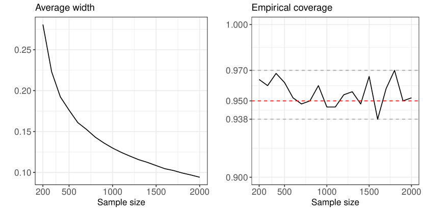
Figure 3: Empirical average width and coverage of the 95% bootstrap confidence interval for the normalized worst risk of $\hat{\beta}_{0.3}$.

6 Normalized worst risk confidence interval via Bootstrap

Equation (12) states that the normalized worst risk of a model $\lim_{\tau\to\infty}\operatorname{\sup_{\operatorname{\tilde{A}}\in\operatorname{C_{1+\tau}}}}\operatorname{R_{\operatorname{{\tilde{A}}}}}(\operatorname{\hat{\beta}_{\lambda}})/\tau$ is equal to its risk stability $\operatorname{R_{\Delta}}(\beta)$. Thus, a confidence interval for the later is a confidence interval for the former. In this section, we construct a bootstrap pivotal confidence interval for $\operatorname{R_{\Delta}}(\beta)$ (Wasserman, 2006).

In order to simplify the notation, let $\hat{\lambda}_{*}$ denote the selected model and assume that we have a fresh sample that is independent from the one used for model selection. Such condition can always be satisfied via sample splitting. Henceforth, let $(\operatorname{\mathbb{X}^{\operatorname{{\tilde{A}}}}},\operatorname{\mathbb{Y}^{\operatorname{{\tilde{A}}}}})$ for $\operatorname{\operatorname{\tilde{A}}\in\{\operatorname{A},\operatorname{0}\}}$ denote the fresh sample, and $(\mathbb{P}^{\operatorname{{0}}},\mathbb{P}^{\operatorname{{A}}})$ the corresponding empirical distributions.

Given a distribution $\mathbb{P}$, let $\mathbb{P}_{b}$ denote a bootstrap resample of $\mathbb{P}$ for $b\in\{1,\dots,B\}$. Then, $\hat{\beta}_{\hat{\lambda}_{*}}^{b}\mathrel{\vbox{\hbox{\scriptsize.}\hbox{\scriptsize.}}}=\hat{\beta}_{\hat{\lambda}_{*}}(\mathbb{P}^{\operatorname{{A}}}_{b},\mathbb{P}^{\operatorname{{0}}}_{b})$ is the selected model refitted in the $b$-bootstrap resample, and $\hat{\beta}_{\hat{\lambda}_{*}}\mathrel{\vbox{\hbox{\scriptsize.}\hbox{\scriptsize.}}}=\hat{\beta}_{\hat{\lambda}_{*}}(\mathbb{P}^{\operatorname{{A}}},\mathbb{P}^{\operatorname{{0}}})$ is the same model refitted in the whole sample. Let $\operatorname{\hat{R}}(\beta,\mathbb{P})$ denote the squared prediction error of the model $\beta$ on the distribution $\mathbb{P}$, we define the risk difference in the $b$-bootstrap resample and the whole sample as

$$\Delta^{b}\mathrel{\vbox{\hbox{\scriptsize.}\hbox{\scriptsize.}}}=\operatorname{\hat{R}}(\hat{\beta}_{\hat{\lambda}_{*}}^{b},\mathbb{P}^{\operatorname{{A}}}_{b})-\operatorname{\hat{R}}(\hat{\beta}_{\hat{\lambda}_{*}}^{b},\mathbb{P}^{\operatorname{{0}}}_{b})\quad\Delta_{n}\mathrel{\vbox{\hbox{\scriptsize.}\hbox{\scriptsize.}}}=\operatorname{\hat{R}}(\hat{\beta}_{\hat{\lambda}_{*}},\mathbb{P}^{\operatorname{{A}}})-\operatorname{\hat{R}}(\hat{\beta}_{\hat{\lambda}_{*}},\mathbb{P}^{\operatorname{{0}}})$$ (39)

An asymptotic $(1-\alpha)$ confidence interval for the normalized work risk is given by the $1-\alpha$ bootstrap pivotal confidence interval of $\Delta$ restricted to the positive real line, that is

$$[0,\infty)\cap(\ 2\Delta_{n}-\Delta_{1-\alpha/2}^{B}\ ,\ 2\Delta_{n}-\Delta_{\alpha/2}^{B}\ )$$ (40)

where $\Delta_{\alpha}^{B}$ is the $\alpha$-quantile of the set $\{\Delta^{b}\}_{b=1}^{B}$. Figure 3 displays the empirical width and coverage of the confidence interval as the sample size is increased. The details of this example are deferred to section 7.2.

7 Simulation studies

In this section, we empirically study causal regularization, and compare it to the causal Dantzig estimator. For all the simulations, the structural matrix $B$ of the structural equation model is displayed in figure 4. In all cases the noise is sampled from a multivariate standard normal. The shift random variable is specified in the following subsections. Moreover, when we mention a sample size $n$, we mean that both the observational and shifted distribution are sampled $n$ times. The code for reproducing the results presented in section 7 and 8 can be found at github.com/lkania/causal-regularization

$$\operatorname{B}=\begin{bmatrix}0&\operatorname{\beta_{PA}}^{T}\\ \operatorname{\beta_{CH}}&\operatorname{B_{X}}\end{bmatrix} \operatorname{\text{ where }}\operatorname{\beta_{PA}}=\begin{bmatrix}0\\ 1\\ 1\\ 0\\ 0\\ 0\\ \end{bmatrix},\ \operatorname{\beta_{CH}}=\begin{bmatrix}0\\ 0\\ 0\\ 1\\ 1\\ 0\\ \end{bmatrix}$$ (41)

$$\operatorname{\text{ and }}\operatorname{B_{X}}=\begin{bmatrix}0&0&0&0&0&0\\ 1&0&0&0&0&0\\ 1&1&0&0&0&0\\ 0&0&0&0&0&0\\ 0&0&0&0&0&0\\ 0&0&0&0&1&0\\ \end{bmatrix}$$ (42)

Figure 4: $\operatorname{SEM}(B,A)$ used for the simulation study.

7.1 Convergence of out-of-sample risk at $O_{p}(1/\sqrt{n})$

Figure 2 displays the empirical and predicted normalized excess risk for $\operatorname{\beta_{PA}}$ (see equation (22)) as the sample size is increased. For every sample size, 1000 experiments are realized and their resulting empirical normalized excess risk averaged. The shifted random variable is chosen as $A\sim\operatorname{{N}}(0,I)$. The computation of the population worst case risk is detailed in appendix B. The fact that the slope of both theoretical and empirical excess risk are the same means that the convergence rate of the empirical risk matches the predicted one.

7.2 Bootstrap confidence interval

Figure 3 presents the empirical width and coverage of the bootstrap confidence intervals for $\hat{\beta}_{0.3}$, proposed in section 6, as the sample size is increased. The shift is taken to be standard normal, $A\sim\operatorname{{N}}(0,I)$, and the corresponding population worst risk computation is detailed in section B of the appendix. For every sample size, 500 repetitions are conducted in order to compute the empirical coverage, and for each experiment 1000 bootstrap resamples were used to compute the confidence interval. We observe that even for small sample sizes, the confidence interval possesses, approximately, the desired coverage.

7.3 Causal regularization vs causal Dantzig

Recall that the causal Dantzig is an extreme point in the regularized path generated by causal regularization. In section 5, we saw that causal regularization coupled with cross-validation will be asymptotically equivalent to the optimal selector. Since by definition, the causal Dantzig minimizes the population worst out-of-sample risk, cross-validation will converge to the causal Dantzig for large sample sizes. Nevertheless, for smaller samples the variance of the causal Dantzig might be so high that its actual out-of-sample risk is less than optimal, whereas other estimators in the causal regularization path perform much better. Figure 5 exemplifies such behaviour. It displays the median normalized out-of-sample risk for out-of-sample datasets that are shifted 10, 100 and 1000 times more than the in-sample datasets. The data is generated from the SEM structure shown in figure 4, and the in-sample shift is given by $A\sim\operatorname{{N}}(0,I)$, while the out-of-sample shifts are chosen as $A\sim\operatorname{{N}}(0,\lambda I)$ such that $\lambda\in\{10,100,1000\}$. The size of both in-sample datasets $n$ are $250$ and $1000$ while the out-of-sample datasets always have sample size $10^{6}$. It is clear that for moderate sample sizes the causal Dantzig estimator can be dramatically improved by causal regularization.

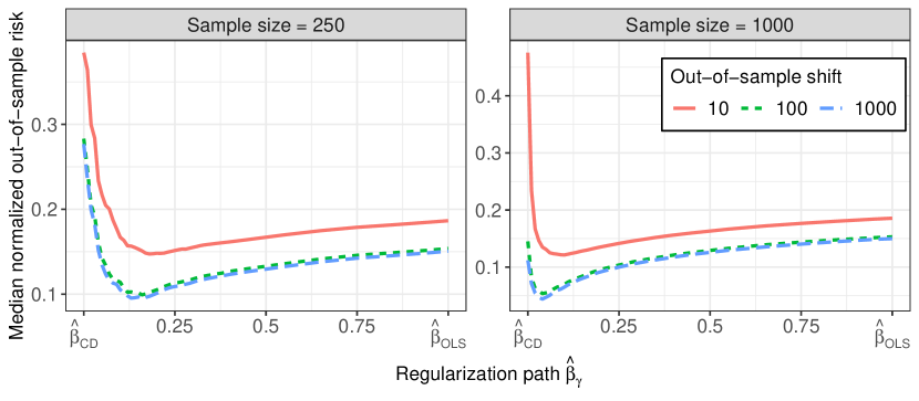
Figure 5: Median normalized risk of the regularization path produced by causal regularization as the out-of-sample datasets are 10, 100 and 1000 times more than the in-sample datasets. Models on the left panel were trained on in-sample datasets consisting of 250 observations while on the right 1000 observation were used. The median was chosen rather than the mean due to the high variance of the causal Dantzig estimator.

Consider the out-of-sample risk of the causal Dantzig and causal regularization as we increase separation between the in-sample distributions, that is, as the magnitude of the in-sample shift is enlarged. Figure 6 compares the in-sample and out-of-sample risk for models obtained via causal regularization and causal Dantzig. All shifted in-sample datasets consist of $n$ examples where the shift was normally distributed i.e., $A\sim\operatorname{{N}}(0,\lambda I)$ such that $\lambda\in\{0.5,1,1.5\}$. Model selection for causal regularization was done by 3-fold cross-validation. As expected, in all cases the out-of-sample risk corresponding to causal regularization is lower than causal Dantzig.

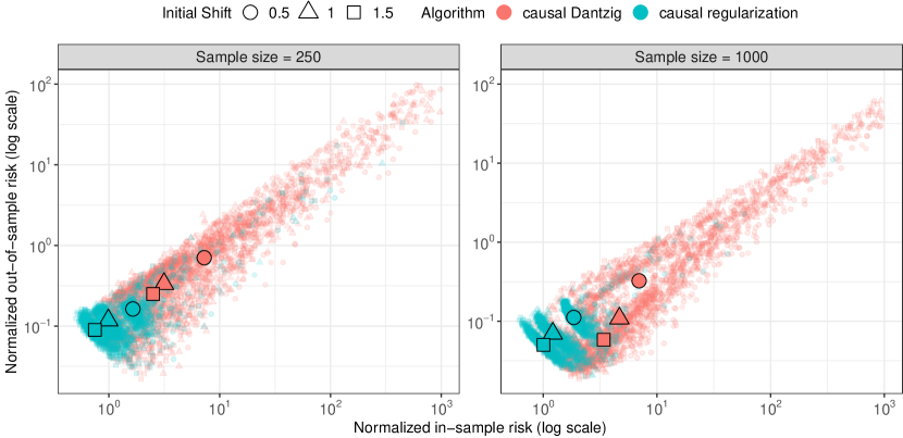
Figure 6: Comparison between causal regularization and the causal Dantzig as the training datasets are progressively shifted. Each faded point is the normalized in-sample and out-of-sample risk achieved by the models. The solid points are medians. The median rather than the mean was chosen due to the high variance of the causal Dantzig estimator.

8 Applications

Below we describe two illustrations of causal regularization in more or less realistic settings. This involves both appropriate transformations of variables, the definition of environments, as well as the definition of the system under consideration.

8.1 Fulton fish market

We apply our methodology to predict the demand in a fish market from the price (Graddy, 1995; Imbens, 2014). In equilibrium, it has been hypothesized that

$$\log(\text{quantity})=\beta_{0}+\beta_{1}\log(\text{price})+\epsilon$$ (43)

where quantity is the daily total quantity of fish in pounds, and price is the average daily price in cents.

We are interested in measuring the prediction quality of the causal regularization and causal Dantzig across the week (Mondays, Tuesdays, Wednesdays and Thursdays). Hence, we split the dataset in a training dataset consisting of Mondays, Tuesdays and Thursdays, and a test dataset composed by Wednesdays. We further divide the training dataset into two datasets: one for stormy days and one for fair days. Stormy days are those when the wind speed is greater than 18 knots and wave height is higher than 4.5 feats. Figure 7 visualizes the covariate and response for each one of the datasets.

We fit causal regularization and the causal Dantzig on the training dataset. Model selection is done by cross-validation with 3 folds. Then, we proceed to compute their risk on 1000 resamples of the test dataset. Figure 8 shows that in each each resample causal regularization obtains a smaller out-of-sample risk than the causal Dantzig.

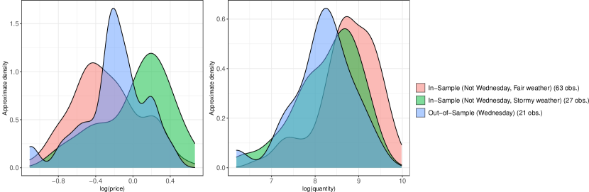
Figure 7: Estimated densities for the amount of fish and its price for each dataset in the Fulton fish market example. This shows that for the covariate, log(price), the observational, fair weather, distribution is indeed different from the shifted, stormy weather, distribution.

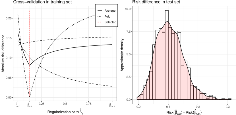
Figure 8: Fulton fish market. (Left) 3-fold cross-validation for causal regularization. The red dashed line indicates the chosen model. (Right) Out-of-sample risk difference between the causal Dantzig and causal regularization. In all cases, the risk achieved by causal regularization is smaller as evidenced by $\text{Risk}(\hat{\beta}_{\text{CD}})-\text{Risk}(\hat{\beta}_{\text{CR}})$ always being positive.

8.2 Gene knockout experiments

Next, we consider a dataset of gene expression in yeast under deletion of single genes (Kemmeren et al., 2014; Meinshausen et al., 2016). There are 262 non-interventional observations, which consists of no gene deletions, and 1479 observations where in each one a different gene is perturbed. In all cases, 6170 genes are measures. The goal is predict the gene expression of one of the genes based on the others. We take as the target the gene that was not directly intervened and whose mean was most shifted between the observation and interventional datasets. Analogously, we choose 10 intervened genes whose mean was most shifted between the interventional and observation datasets as the predictors.

We analyze the performance of causal regularization and the causal Dantzig by nested cross-validation. The interventional data was split in 25 folds; of those 24 were used as a training set, and the remaining as a test set. On the training set, model selection was done via 5-fold cross-validation. Finally, the risk of the estimator was evaluated in the test set. Figure 1 displays the cross-validation selection and the corresponding point in the coefficient path for one of the iterations. The process was repeated leaving one of the 25 folds out at a time. The right-lower pane of figure 1 shows that in all cases, causal regularization achieved a smaller risk than the causal Dantzig.

9 Conclusion

In this paper, we have introduced causal regularization, a technique for trading off in-sample and out-of-sample risk guarantees by exploiting the heterogeneity across in-sample datasets. The method provides out-of-sample guarantees, for any regularization parameter, against specific covariates shifts in the same sense as the causal Dantzig estimator while being identifiable in a broader set of circumstances. Furthermore, we showed theoretically and empirically that cross-validation and sample-splitting can be used to do model selection for causal regularization, and obtain estimators with better out-of-sample performance than the causal Dantzig estimator.

The ideas developed in this work can be extended to some generalized linear models by appropriately defining the risk so that we have risk stability under the causal model. For instance, consider the Poisson regression analogue of definition 1: $\operatorname{Y^{\operatorname{{A}}}}|\operatorname{X^{\operatorname{{A}}}}\sim\text{Poisson}(m(\beta))$ where $m(\beta)\mathrel{\vbox{\hbox{\scriptsize.}\hbox{\scriptsize.}}}=\exp(\beta^{T}\operatorname{X^{\operatorname{{A}}}})$, and consider the Pearson $\chi^{2}$-risk: $\operatorname{R_{\operatorname{{A}}}}(\beta)\mathrel{\vbox{\hbox{\scriptsize.}\hbox{\scriptsize.}}}=\operatorname{\mathbb{E}}\left[(\operatorname{Y^{\operatorname{{A}}}}-m(\beta))^{2}/m(\beta)\right]$. It follows that $\operatorname{R_{\operatorname{{A}}}}(\operatorname{\beta_{PA}})$ is constant w.r.t. A, thus we can use causal regularization, as in equation (3), to trade-off overall in-sample fit for risk stability across sub-samples. The out-of-sample risk guarantees are, however, not trivial to derive due to the non-linearity and require further assumptions.

Causal regularization is effective against additive covariate shifts, as specified in definition 1. If the shift between datasets does not follow this pattern, then causal regularization only protects against the projection of the shift to the set of additive shifts.

Acknowledgement

The authors acknowledge funding from the Swiss National Science Foundation (SNSF 188534).

Appendix A Proofs

A.1 Population statements

See 1

Proof.

Let $\operatorname{\operatorname{\tilde{A}}}\in C_{1+\tau}$, by the SEM definition 1, it holds that

$$\begin{bmatrix}\operatorname{Y^{\operatorname{{\tilde{A}}}}}\\ \operatorname{X^{\operatorname{{\tilde{A}}}}}\end{bmatrix}=(I-B)^{-1}\left(\epsilon+\begin{bmatrix}0\\ \operatorname{\operatorname{\tilde{A}}}\end{bmatrix}\right)$$ (44)

Let $\operatorname{P_{X}}\in\operatorname{\mathbb{R}}^{p\times(p+1)}$ and $\operatorname{P_{Y}}\in\operatorname{\mathbb{R}}^{1\times(p+1)}$ be the projections of the $X$ and $Y$ coordinates, i.e., $\operatorname{P_{X}}=\begin{bmatrix}\operatorname{\mathbb{0}}_{p\times 1}&I_{p\times p}\end{bmatrix}$ and $\operatorname{P_{Y}}=\begin{bmatrix}1&\operatorname{\mathbb{0}}_{1\times p}\end{bmatrix}$, the population residuals can be rewritten as a projection of equation (44)

$$\operatorname{Y^{\operatorname{{\tilde{A}}}}}-\beta^{T}\operatorname{X^{\operatorname{{\tilde{A}}}}}=u\left(\epsilon+\begin{bmatrix}0\\ \operatorname{\operatorname{\tilde{A}}}\end{bmatrix}\right)\quad\operatorname{\text{ where }}u\mathrel{\vbox{\hbox{\scriptsize.}\hbox{\scriptsize.}}}=(\operatorname{P_{Y}}-\beta^{T}\operatorname{P_{X}})(I-B)^{-1}$$ (45)

It follows that the residuals under the shift $\operatorname{\operatorname{\tilde{A}}}$ are

$$\operatorname{R_{\operatorname{{\tilde{A}}}}}(\beta)=\operatorname{\mathbb{E}}[(\operatorname{Y^{\operatorname{{\tilde{A}}}}}-\beta^{T}\operatorname{X^{\operatorname{{\tilde{A}}}}})^{2}]=u\left(\operatorname{\mathbb{C}}[\epsilon]+\begin{bmatrix}0&\operatorname{\mathbb{0}}^{T}\\ \operatorname{\mathbb{0}}&\operatorname{\operatorname{\mathbb{E}}[\operatorname{\operatorname{\tilde{A}}}\operatorname{\operatorname{\tilde{A}}}^{T}]}\end{bmatrix}\right)u^{T}$$ (46)

where we have exploited the fact that the shift variable and the noise are uncorrelated, i.e., $\operatorname{\mathbb{C}}[\operatorname{\tilde{A}},\epsilon]=0$. Taking the supremum over $C_{1+\tau}$, we obtain

$$\operatorname{\sup_{\operatorname{\tilde{A}}\in\operatorname{C_{1+\tau}}}}\operatorname{R_{\operatorname{{\tilde{A}}}}}(\beta)=u\left(\operatorname{\mathbb{C}}[\epsilon]+(1+\tau)\begin{bmatrix}0&\operatorname{\mathbb{0}}^{T}\\ \operatorname{\mathbb{0}}&\operatorname{\operatorname{\mathbb{E}}[\operatorname{\operatorname{A}}\operatorname{\operatorname{A}}^{T}]}\end{bmatrix}\right)u^{T}$$ (47)

Noting that equation (46) implies that

$$\operatorname{R_{\Delta}}(\beta)=u\left(\begin{bmatrix}0&\operatorname{\mathbb{0}}^{T}\\ \operatorname{\mathbb{0}}&\operatorname{\operatorname{\mathbb{E}}[\operatorname{\operatorname{A}}\operatorname{\operatorname{A}}^{T}]}\end{bmatrix}\right)u^{T}$$ (48)

and replacing it back into equation (47), we get

$$\operatorname{\sup_{\operatorname{\tilde{A}}\in\operatorname{C_{1+\tau}}}}\operatorname{R_{\operatorname{{\tilde{A}}}}}(\beta)=\operatorname{R_{\operatorname{{A}}}}(\beta)+\tau\operatorname{R_{\Delta}}(\beta)=\frac{1}{2}\operatorname{\operatorname{R_{+}}}(\beta)+\frac{1+2\tau}{2}\operatorname{R_{\Delta}}(\beta)$$ (49)

∎

Proposition 3.

$\operatorname{G_{\Delta}}$ is positive semi-definite and $\operatorname{rank}\operatorname{G_{\Delta}}=\operatorname{rank}\operatorname{\operatorname{\mathbb{E}}[\operatorname{\operatorname{A}}\operatorname{\operatorname{A}}^{T}]}$

Proof.

By definition

$$\operatorname{G_{\Delta}}=\operatorname{\operatorname{\mathbb{E}}[\operatorname{X^{\operatorname{{A}}}}\operatorname{{X^{\operatorname{{A}}}}^{T}}]}-\operatorname{\operatorname{\mathbb{E}}[\operatorname{X^{\operatorname{{0}}}}\operatorname{{X^{\operatorname{{0}}}}^{T}}]}$$ (50)

Let $\operatorname{P_{X}}\in\operatorname{\mathbb{R}}^{p\times(p+1)}$ be the projection of the $X$ coordinates, i.e., $\operatorname{P_{X}}=\begin{bmatrix}\operatorname{\mathbb{0}}_{p\times 1}&I_{p\times p}\end{bmatrix}$, then for $\operatorname{\operatorname{\tilde{A}}\in\{\operatorname{A},\operatorname{0}\}}$

$$\operatorname{\operatorname{\mathbb{E}}[\operatorname{X^{\operatorname{{\tilde{A}}}}}\operatorname{{X^{\operatorname{{\tilde{A}}}}}^{T}}]}=u\left(\operatorname{\mathbb{C}}[\epsilon]+\begin{bmatrix}0&\operatorname{\mathbb{0}}^{T}\\ \operatorname{\mathbb{0}}&\operatorname{\operatorname{\mathbb{E}}[\operatorname{\operatorname{\tilde{A}}}\operatorname{\operatorname{\tilde{A}}}^{T}]}\end{bmatrix}\right)u^{T}\operatorname{\text{ where }}u=\operatorname{P_{X}}(I-B)^{-1}$$ (51)

since $\operatorname{\mathbb{C}}[\operatorname{\tilde{A}},\epsilon]=0$. Let $(I-B)^{-1}\mathrel{\vbox{\hbox{\scriptsize.}\hbox{\scriptsize.}}}=\begin{bmatrix}1&v^{T}\\ w&M\\ \end{bmatrix}$, then $u=\operatorname{P_{X}}(I-B)^{-1}=\begin{bmatrix}w&M\end{bmatrix}$ and

$$\operatorname{\operatorname{\mathbb{E}}[\operatorname{X^{\operatorname{{\tilde{A}}}}}\operatorname{{X^{\operatorname{{\tilde{A}}}}}^{T}}]}=u\operatorname{\mathbb{C}}[\epsilon]u^{T}+M\operatorname{\operatorname{\mathbb{E}}[\operatorname{\operatorname{\tilde{A}}}\operatorname{\operatorname{\tilde{A}}}^{T}]}M^{T}$$ (52)

Thus, $\operatorname{G_{\Delta}}=M\operatorname{\operatorname{\mathbb{E}}[\operatorname{\operatorname{A}}\operatorname{\operatorname{A}}^{T}]}M^{T}$. We can explicitly write the inverse of $M$ by noting that

$$(I-B)^{-1}(I-B)=I_{(p+1)\times(p+1)} \implies\begin{cases}-w\operatorname{\beta_{PA}}^{T}+M(I-B_{X})&=I_{p\times p}\\ w-M\operatorname{\beta_{CH}}&=\operatorname{\mathbb{0}}\end{cases}$$ (53)

$$\implies M\left((I-\operatorname{B_{X}})-\operatorname{\beta_{CH}}\operatorname{\beta_{PA}}^{T}\right)=I_{p\times p}$$ (54)

Thus, $M$ is square and has a right-inverse, hence $M$ is invertible. In other words, $M$ is a product of elementary matrices and doens’t modify the column-rank or the row-rank of any conformal matrix. Ergo,

$$\operatorname{rank}\operatorname{G_{\Delta}} =\operatorname{rank}M\operatorname{\operatorname{\mathbb{E}}[\operatorname{\operatorname{A}}\operatorname{\operatorname{A}}^{T}]}M^{T}=\operatorname{rank}\operatorname{\operatorname{\mathbb{E}}[\operatorname{\operatorname{A}}\operatorname{\operatorname{A}}^{T}]}$$ (55)

Finally, note that under the assumption that $\operatorname{\operatorname{\mathbb{E}}[\operatorname{\operatorname{A}}\operatorname{\operatorname{A}}^{T}]}$ is positive semi-definite, it follows that $\operatorname{G_{\Delta}}$ is positive semi-definite since

$$\forall\beta\in\operatorname{\mathbb{R}^{p}}\beta^{T}\operatorname{G_{\Delta}}\beta=(M^{T}\beta)^{T}\operatorname{\operatorname{\mathbb{E}}[\operatorname{\operatorname{A}}\operatorname{\operatorname{A}}^{T}]}(M^{T}\beta)\geq 0$$ (56)

∎

Proposition 4 (The risk difference is a centred quadratic form).

$$\forall\beta\in\operatorname{\mathbb{R}^{p}}\ \operatorname{R_{\Delta}}(\beta)=(\beta-\operatorname{\beta_{PA}})^{T}\operatorname{G_{\Delta}}(\beta-\operatorname{\beta_{PA}})$$ (57)

Proof.

For $\operatorname{\operatorname{\tilde{A}}\in\{\operatorname{A},\operatorname{0}\}}$

$$\operatorname{R_{\operatorname{{\tilde{A}}}}}(\beta)=\operatorname{\mathbb{E}}[(\operatorname{Y^{\operatorname{{\tilde{A}}}}}-\beta^{T}\operatorname{X^{\operatorname{{\tilde{A}}}}})^{2}]=\beta^{T}\operatorname{\operatorname{\mathbb{E}}[\operatorname{X^{\operatorname{{\tilde{A}}}}}\operatorname{{X^{\operatorname{{\tilde{A}}}}}^{T}}]}\beta-2\beta^{T}\operatorname{\operatorname{\mathbb{E}}[\operatorname{X^{\operatorname{{\tilde{A}}}}}\operatorname{Y^{\operatorname{{\tilde{A}}}}}]}+\operatorname{\operatorname{\mathbb{E}}[\operatorname{(Y^{\operatorname{{\tilde{A}}}})^{2}}]}$$ (58)

Recalling the definitions

$$\operatorname{G_{\Delta}} =\operatorname{\operatorname{\mathbb{E}}[\operatorname{X^{\operatorname{{A}}}}\operatorname{{X^{\operatorname{{A}}}}^{T}}]}-\operatorname{\operatorname{\mathbb{E}}[\operatorname{X^{\operatorname{{0}}}}\operatorname{{X^{\operatorname{{0}}}}^{T}}]}$$ (59)

$$\operatorname{Z_{\Delta}} =\operatorname{\operatorname{\mathbb{E}}[\operatorname{X^{\operatorname{{A}}}}\operatorname{Y^{\operatorname{{A}}}}]}-\operatorname{\operatorname{\mathbb{E}}[\operatorname{X^{\operatorname{{0}}}}\operatorname{Y^{\operatorname{{0}}}}]}=\operatorname{G_{\Delta}}\operatorname{\beta_{PA}}$$ By equation (4)

It holds that

$$\operatorname{R_{\Delta}}(\beta) =\operatorname{R_{\operatorname{{A}}}}(\beta)-\operatorname{R_{\operatorname{{0}}}}(\beta)$$ (60)

$$=\beta^{T}\operatorname{G_{\Delta}}\beta-2\beta^{T}\operatorname{G_{\Delta}}\operatorname{\beta_{PA}}+\operatorname{\operatorname{\mathbb{E}}[(\operatorname{Y^{\operatorname{{A}}}})^{2}]}-\operatorname{\operatorname{\mathbb{E}}[(\operatorname{Y^{\operatorname{{0}}}})^{2}]}$$ (61)

Notice that for $\operatorname{\operatorname{\tilde{A}}\in\{\operatorname{A},\operatorname{0}\}}$, $\operatorname{\operatorname{\mathbb{E}}[\operatorname{(Y^{\operatorname{{\tilde{A}}}})^{2}}]}$ can be expanded as follows

$$\operatorname{\operatorname{\mathbb{E}}[\operatorname{(Y^{\operatorname{{\tilde{A}}}})^{2}}]} =\operatorname{\mathbb{E}}[(\operatorname{\beta_{PA}^{T}}\operatorname{X^{\operatorname{{\tilde{A}}}}}+\epsilon_{Y})^{2}]$$ (62)

$$=\operatorname{\beta_{PA}^{T}}\operatorname{\operatorname{\mathbb{E}}[\operatorname{X^{\operatorname{{\tilde{A}}}}}\operatorname{{X^{\operatorname{{\tilde{A}}}}}^{T}}]}\operatorname{\beta_{PA}}+\operatorname{\mathbb{E}}[\epsilon_{Y}^{2}]+\operatorname{\beta_{PA}^{T}}\operatorname{\mathbb{E}}[\operatorname{X^{\operatorname{{\tilde{A}}}}}\epsilon_{Y}]$$ (63)

$$=\operatorname{\beta_{PA}^{T}}\operatorname{\operatorname{\mathbb{E}}[\operatorname{X^{\operatorname{{\tilde{A}}}}}\operatorname{{X^{\operatorname{{\tilde{A}}}}}^{T}}]}\operatorname{\beta_{PA}}+\operatorname{\mathbb{E}}[\epsilon_{Y}^{2}]+\operatorname{\beta_{PA}^{T}}u\operatorname{\mathbb{E}}[(\epsilon+\operatorname{\tilde{A}})\epsilon_{Y}]$$ (64)

$$=\operatorname{\beta_{PA}^{T}}\operatorname{\operatorname{\mathbb{E}}[\operatorname{X^{\operatorname{{\tilde{A}}}}}\operatorname{{X^{\operatorname{{\tilde{A}}}}}^{T}}]}\operatorname{\beta_{PA}}+\operatorname{\mathbb{E}}[\epsilon_{Y}^{2}]+\operatorname{\beta_{PA}^{T}}u\operatorname{\mathbb{C}}[\epsilon,\epsilon_{Y}] \operatorname{\mathbb{E}}[\operatorname{\tilde{A}}\epsilon_{Y}]=0$$ since

hence

$$\operatorname{\operatorname{\mathbb{E}}[(\operatorname{Y^{\operatorname{{A}}}})^{2}]}-\operatorname{\operatorname{\mathbb{E}}[(\operatorname{Y^{\operatorname{{0}}}})^{2}]}=\operatorname{\beta_{PA}^{T}}\operatorname{G_{\Delta}}\operatorname{\beta_{PA}}$$ (66)

plugging the result back into equation (61), we get

$$\operatorname{R_{\Delta}}(\beta) =\beta^{T}\operatorname{G_{\Delta}}\beta+\beta^{T}\operatorname{G_{\Delta}}\operatorname{\beta_{PA}}+\operatorname{\beta_{PA}^{T}}\operatorname{G_{\Delta}}\operatorname{\beta_{PA}}$$ (67)

$$=(\beta-\operatorname{\beta_{PA}})^{T}\operatorname{G_{\Delta}}(\beta-\operatorname{\beta_{PA}})$$ (68)

∎

Theorem 1 (Moore–Penrose inverse).

Given a $A\in\operatorname{\mathbb{R}}^{p\times p}$, the Moore–Penrose inverse $A$ is defined as the unique matrix $A^{g}\in\operatorname{\mathbb{R}}^{p\times p}$ that satisfies the following properties

$$A^{g}AA^{g} =A$$ (1)

$$AA^{g}A =A$$ (2)

$$(AA^{g})^{T} =AA^{g}$$ (3)

$$(A^{g}A)^{T} =A^{g}A$$ (4)

See 1

Proof.

Note that

$$\operatorname{R_{\Delta}}(\beta)=(\beta-\operatorname{\beta_{PA}})^{T}\operatorname{G_{\Delta}}(\beta-\operatorname{\beta_{PA}})=\left\lVert\operatorname{G_{\Delta}^{1/2}}(\beta-\operatorname{\beta_{PA}})\right\rVert_{2}^{2}$$ (69)

where the first equality holds by proposition 4, and in the last equality we applied the square root definition. The existence of $\operatorname{G_{\Delta}^{1/2}}$ positive semi-definite is guaranteed by the positive semi-definiteness of $\operatorname{G_{\Delta}}$, see proposition 3. Let $\operatorname{G_{\Delta}^{g/2}}$ be the pseudoinverse of $\operatorname{G_{\Delta}^{1/2}}$, we rewrite the regularizer as follows,

$$\operatorname{G_{\Delta}^{1/2}} =\operatorname{G_{\Delta}^{1/2}}\operatorname{G_{\Delta}^{g/2}}\operatorname{G_{\Delta}^{1/2}}$$ by theorem 1.2

$$=(\operatorname{G_{\Delta}^{1/2}}\operatorname{G_{\Delta}^{g/2}})^{T}\operatorname{G_{\Delta}^{1/2}}$$ by theorem 1.3

$$=(\operatorname{G_{\Delta}^{g/2}})^{T}(\operatorname{G_{\Delta}^{1/2}})^{T}\operatorname{G_{\Delta}^{1/2}}$$ (70)

$$=(\operatorname{G_{\Delta}^{g/2}})^{T}\operatorname{G_{\Delta}}$$ by square root def.

plugging the result back into equation (69), and using equation (4) in the last equality, we get

$$\operatorname{R_{\Delta}}(\beta)=\left\lVert(\operatorname{G_{\Delta}^{g/2}})^{T}(\operatorname{G_{\Delta}}\beta-\operatorname{G_{\Delta}}\operatorname{\beta_{PA}})\right\rVert_{2}^{2}=\left\lVert(\operatorname{G_{\Delta}^{g/2}})^{T}(\operatorname{G_{\Delta}}\beta-\operatorname{Z_{\Delta}})\right\rVert_{2}^{2}$$ (71)

∎

See 1

Proof.

For $\lambda\in\operatorname{[0,\infty)}$

$$\operatorname{\beta_{\lambda}} \mathrel{\vbox{\hbox{\scriptsize.}\hbox{\scriptsize.}}}=\operatorname*{arg\,min}_{\beta\in\operatorname{\mathbb{R}^{p}}}\frac{1}{2}\operatorname{R_{+}}(\beta)+\frac{\lambda}{2}\operatorname{R_{\Delta}}(\beta)$$ (72)

$$=\operatorname*{arg\,min}_{\beta\in\operatorname{\mathbb{R}^{p}}}\frac{1}{2}\beta^{T}\operatorname{G_{\lambda}}\beta-\beta^{T}(\operatorname{Z_{+}}+\lambda\operatorname{G_{\Delta}}\operatorname{\beta_{PA}})$$ by proposition 4

$$=\operatorname*{arg\,min}_{\beta\in\operatorname{\mathbb{R}^{p}}}\frac{1}{2}\beta^{T}\operatorname{G_{\lambda}}\beta-\beta^{T}(\operatorname{Z_{+}}+\lambda\operatorname{Z_{\Delta}})$$ by equation 4

$$=\operatorname{G_{\lambda}^{-1}}\operatorname{Z_{\lambda}}$$ (73)

Note that $\operatorname{G_{\lambda}^{-1}}$ always exists since $\operatorname{G_{\lambda}}$ is positive definite because $\operatorname{G_{+}}$ is assumed non-singular, and therefore positive definite, and $\operatorname{G_{\Delta}}$ is positive semi-definite by proposition 3. Given the uniqueness of the solution, we can express $\operatorname{\beta_{\lambda}}$ as the least squares solution of $\operatorname{G_{\lambda}}\beta=\operatorname{Z_{\lambda}}$, i.e. $\operatorname{\beta_{\lambda}}\mathrel{\vbox{\hbox{\scriptsize.}\hbox{\scriptsize.}}}=\operatorname*{arg\,min}_{\beta\in\operatorname{\mathbb{R}^{p}}}\left\lVert\operatorname{G_{\lambda}}\beta-\operatorname{Z_{\lambda}}\right\rVert_{2}$. Finally, if $\operatorname{G_{\Delta}}$ is full rank, $\beta_{\infty}=\operatorname*{arg\,min}_{\beta\in\operatorname{\mathbb{R}^{p}}}\left\lVert\operatorname{G_{\Delta}}\beta-\operatorname{Z_{\Delta}}\right\rVert_{2}$, that is, causal regularization at $\gamma=\infty$ and the causal Dantzig have the same solution, see equation (5).

∎

A.2 Consistency

Definition 5.

Let $A\in\operatorname{\mathbb{R}}^{p\times p}$ be a symmetric matrix, its operator norm can be defined as

$$\left\lVert A\right\rVert_{2}\mathrel{\vbox{\hbox{\scriptsize.}\hbox{\scriptsize.}}}=\max_{x\in\operatorname{\mathbb{R}^{p}}\operatorname{\text{ s.t. }}\left\lVert x\right\rVert_{2}\leq 1}|x^{T}Ax|$$ (74)

and it holds that

$$\left\lVert A\right\rVert_{2}=\max_{1\leq i\leq p}|\gamma_{i}(A)|$$ (75)

where $\gamma_{i}(A)$ is the $i$-th eigenvalue of $A$.

Theorem 2 (Stewart [1977], Theorem 3.3).

Let $A\in\operatorname{\mathbb{R}}^{p\times p}$ and $B\in\operatorname{\mathbb{R}}^{p\times p}$, then

$$\left\lVert A^{g}-B^{g}\right\rVert_{2}\leq C\cdot\max\{\left\lVert A^{g}\right\rVert_{2}^{2},\left\lVert B^{g}\right\rVert_{2}^{2}\}\cdot\left\lVert A-B\right\rVert_{2}^{2}$$ (76)

where $A$, $\left\lVert\cdot\right\rVert_{2}$ denotes the opetor norm, and $C$ is a positive universal constant.

Lemma 4.

Let $A\in\operatorname{\mathbb{R}}^{p\times p}$ be a positive symmetric define matrix, and $\{B_{n}\}_{n=1}^{\infty}\in\operatorname{\mathbb{R}}^{p\times p}$ a sequence of symmetric matrices such that $\left\lVert A-B_{n}\right\rVert_{2}\operatorname{\overset{p}{\to}}0$, then $\left\lVert A^{g}-B_{n}^{g}\right\rVert_{2}\operatorname{\overset{p}{\to}}0$

Proof.

By theorem 2, it holds that

$$\left\lVert A^{g}-B_{n}^{g}\right\rVert_{2}\leq C\cdot\max\{\left\lVert A^{g}\right\rVert_{2}^{2},\left\lVert B_{n}^{g}\right\rVert_{2}^{2}\}\cdot\left\lVert A-B_{n}\right\rVert_{2}^{2}$$ (77)

Since $A$ is a positive symmetric definite matrix, it has an inverse, and it follows that

$$\left\lVert A^{g}\right\rVert_{2}=\left\lVert A^{-1}\right\rVert_{2}=\gamma_{\min}(A)^{-1}$$ (78)

where $\gamma_{\min}(A)$ is the smallest positive eigenvalue of $A$. Let $UDV^{T}$ be the SVD decomposition of $B_{n}$, it holds that

$$B_{n}^{g}=UD^{g}V^{T}\operatorname{\text{ where }}\gamma_{i}(D^{g})=\begin{cases}0&\text{ if }\gamma_{i}(B_{n})=0\\ |\gamma_{i}(B_{n})|^{-1}&\text{ otherwise }\end{cases}$$ (79)

and we rewrite the operator norm of $B_{n}$ as

$$\left\lVert B_{n}^{g}\right\rVert_{2}=\left\lVert UD^{g}V^{T}\right\rVert_{2}=\left\lVert D^{g}\right\rVert_{2}=\begin{cases}0&\text{ if }\gamma_{i}(B_{n})=0\ \forall 1\leq i\leq p\\ \max\{\ |\gamma_{i}(B_{n})|^{-1}\operatorname{\text{ s.t. }}|\gamma_{i}(B_{n})|>0\ \}\ &\text{otherwise}\end{cases}$$ (80)

where the second equality is due to the operator norm being unitarily invariant.

Weyl’s inequality says that if $B_{n}$ converges to $A$ in operator norm, then their eigenvalues converge uniformly,

$$|\ \gamma_{i}(A)-|\gamma_{i}(B_{n})|\ |\leq|\gamma_{i}(A)-\gamma_{i}(B_{n})|\leq\left\lVert A-B_{n}\right\rVert_{2}\quad\operatorname{\text{ for }}1\leq i\leq p$$ (81)

Thus, a lowerbound for $|\gamma_{i}(B)|$ is

$$\gamma_{\min}(A)-\left\lVert A-B_{n}\right\rVert_{2}\leq\gamma_{i}(A)-\left\lVert A-B_{n}\right\rVert_{2}\leq|\gamma_{i}(B_{n})|\quad\operatorname{\text{ for }}1\leq i\leq p$$ (82)

Define the event $E_{n}$ as

$$E_{n}\ \mathrel{\vbox{\hbox{\scriptsize.}\hbox{\scriptsize.}}}=\ \{\gamma_{\min}(A)-\left\lVert A-B_{n}\right\rVert_{2}>0\}$$ (83)

it follows that on the event $E_{n}$,

$$\left\lVert B_{n}^{g}\right\rVert_{2}\leq\frac{1}{\gamma_{\min}(A)-\left\lVert A-B_{n}\right\rVert_{2}}$$ (84)

Hence, if the event $E_{n}$ happens, it holds that

$$\left\lVert A^{g}-B_{n}^{g}\right\rVert_{2} \leq C\cdot\max\{\frac{1}{\gamma_{\min}(A)^{2}},\frac{1}{(\gamma_{\min}(A)-\left\lVert A-B_{n}\right\rVert_{2})^{2}}\}\cdot\left\lVert A-B_{n}\right\rVert_{2}^{2}$$ (85)

$$\leq g(\left\lVert A-B_{n}\right\rVert_{2})\quad\operatorname{\text{ where }}g(x)\mathrel{\vbox{\hbox{\scriptsize.}\hbox{\scriptsize.}}}=\frac{x^{2}}{(\gamma_{\min}(A)-x)^{2}}$$ (86)

Putting all together we get that for $\epsilon>0\operatorname{\text{ and }}\delta>0$

$$P(\left\lVert A^{g}-B_{n}^{g}\right\rVert_{2}\geq\epsilon) =P(\ \left\lVert A^{g}-B_{n}^{g}\right\rVert_{2}\geq\epsilon\land E_{n}\ )+P(\ \left\lVert A^{g}-B_{n}^{g}\right\rVert_{2}\geq\epsilon\land E_{n}^{c}\ )$$ (87)

$$\leq P(\ g(\left\lVert A-B_{n}\right\rVert_{2})>\epsilon\ )+P(\ E_{n}^{c}\ )$$ (88)

$$=P(\ g(\left\lVert A-B_{n}\right\rVert_{2})>\epsilon\ )+P(\ \left\lVert A-B_{n}\right\rVert_{2}\geq\gamma_{\min}(A)\ )$$ (89)

Where the inequality is due to equation (86). Note that $g$ is continuous for $x\not=\gamma_{\min}(A)$ and $g(0)=0$. Since $\left\lVert A-B_{n}\right\rVert_{2}\operatorname{\overset{p}{\to}}0$ and $\gamma_{\min}(A)>0$, by the continuous mapping theorem $g(\left\lVert A-B_{n}\right\rVert_{2})\operatorname{\overset{p}{\to}}0$. Hence, we can choose $N\mathrel{\vbox{\hbox{\scriptsize.}\hbox{\scriptsize.}}}=N(\epsilon,\gamma_{\min}(A),\delta)\in\mathbb{N}$ such that $P(\ g(\left\lVert A-B_{n}\right\rVert_{2})>\epsilon\ )<\frac{\delta}{2}$ and $P(\ \left\lVert A-B_{n}\right\rVert_{2}\geq\gamma_{\min}(A)\ )<\frac{\delta}{2}$ for all $n\geq N$, which implies that $P(\left\lVert A^{g}-B_{n}^{g}\right\rVert_{2}\geq\epsilon)<\delta$ for all $n\geq N$ and consequently $\left\lVert A^{g}-B_{n}^{g}\right\rVert_{2}\operatorname{\overset{p}{\to}}0$

∎

See 2

Proof.

By the weak law of large numbers and continuity, $\operatorname{\mathbb{G}_{+}}$, $\operatorname{\mathbb{G}_{\Delta}}$, $\operatorname{\mathbb{Z}_{+}}$, and $\operatorname{\mathbb{Z}_{\Delta}}$ converge in probability to $\operatorname{G_{+}}$, $\operatorname{G_{\Delta}}$, $\operatorname{Z_{+}}$, and $\operatorname{Z_{\Delta}}$ correspondingly. Hence, by continuity, $\operatorname{\mathbb{G}_{\lambda}}\mathrel{\vbox{\hbox{\scriptsize.}\hbox{\scriptsize.}}}=\operatorname{\mathbb{G}_{+}}+\lambda\operatorname{\operatorname{\mathbb{G}_{\Delta}}}$ and $\operatorname{\mathbb{Z}_{\lambda}}\mathrel{\vbox{\hbox{\scriptsize.}\hbox{\scriptsize.}}}=\operatorname{\mathbb{Z}_{+}}+\lambda\operatorname{\operatorname{\mathbb{Z}_{\Delta}}}$ converge in probability to $\operatorname{G_{\lambda}}$ and $\operatorname{Z_{\lambda}}$.

Since $p$ is finite, $\operatorname{\mathbb{G}_{\lambda}}\operatorname{\overset{p}{\to}}\operatorname{G_{\lambda}}$ implies $\left\lVert\operatorname{G_{\lambda}}-\operatorname{\mathbb{G}_{\lambda}}\right\rVert_{2}\operatorname{\overset{p}{\to}}0$. Then, theorem 2 implies that $\left\lVert\operatorname{G_{\lambda}^{g}}-\operatorname{\mathbb{G}_{\lambda}^{g}}\right\rVert_{2}\operatorname{\overset{p}{\to}}0$, and consequently $\operatorname{\mathbb{G}_{\lambda}^{g}}\operatorname{\overset{p}{\to}}\operatorname{G_{\lambda}^{g}}$. It follows that

$$\operatorname{\hat{\beta}_{\lambda}}\mathrel{\vbox{\hbox{\scriptsize.}\hbox{\scriptsize.}}}=\operatorname{\mathbb{G}_{\lambda}^{g}}\operatorname{\mathbb{Z}_{\lambda}}\operatorname{\overset{p}{\to}}\operatorname{G_{\lambda}^{g}}\operatorname{Z_{\lambda}}=\operatorname{G_{\lambda}^{-1}}\operatorname{Z_{\lambda}}=\operatorname{\beta_{\lambda}}$$ (90)

where the convergence in probability is due to continuity, and the penultimate equality is due to $\operatorname{G_{\lambda}}$ being positive definite since $\operatorname{G_{+}}$ is assumed positive definite, and $\operatorname{G_{\Delta}}$ is positive semi-definite by proposition 3.

∎

A.3 Finite sample bounds

Proposition 5.

For $\operatorname{\operatorname{\tilde{A}}\in\operatorname{{A}}}$,

$$|\operatorname{R_{\operatorname{{\tilde{A}}}}}(\beta)-\operatorname{\hat{R}_{\operatorname{{\tilde{A}}}}}(\beta)|\leq(\left\lVert\beta\right\rVert_{1}^{2}+1)\operatorname{\mathbb{V}}[\operatorname{Y^{\operatorname{{\tilde{A}}}}}]\left(\max_{1\leq k\leq p}\operatorname{\mathbb{V}}[\operatorname{X^{\operatorname{{\tilde{A}}}}_{k}}]\right)\left(\sqrt{\frac{4q+8\log(p)}{n_{\operatorname{{\tilde{A}}}}}}+\frac{4q+8\log(p)}{n_{\operatorname{{\tilde{A}}}}}\right)$$ (91)

with probability exceeding $1-2e^{-q}$ for $q>0$, hence $|\operatorname{R_{\operatorname{{\tilde{A}}}}}(\beta)-\operatorname{\hat{R}_{\operatorname{{\tilde{A}}}}}(\beta)|=o_{p}\left(\frac{1}{\sqrt{n_{\operatorname{{\tilde{A}}}}}}\right)$

Proof.

Let $\operatorname{V^{\operatorname{{\tilde{A}}}}}\mathrel{\vbox{\hbox{\scriptsize.}\hbox{\scriptsize.}}}=\begin{bmatrix}\operatorname{Y^{\operatorname{{\tilde{A}}}}}\\ \operatorname{X^{\operatorname{{\tilde{A}}}}}\end{bmatrix}$, $\operatorname{S^{\operatorname{{\tilde{A}}}}}=\operatorname{\mathbb{E}}[\operatorname{V^{\operatorname{{\tilde{A}}}}}\operatorname{V^{\operatorname{{\tilde{A}}}}}^{T}]$, and $\upsilon\mathrel{\vbox{\hbox{\scriptsize.}\hbox{\scriptsize.}}}=\begin{bmatrix}-1\\ \beta\end{bmatrix}$ then

$$|\operatorname{R_{+}}(\beta)-\operatorname{\hat{R}_{+}}(\beta)|=|\upsilon^{T}(\operatorname{\hat{S}^{\operatorname{{\tilde{A}}}}}-\operatorname{S^{\operatorname{{\tilde{A}}}}})\upsilon|\leq\left\lVert\upsilon\right\rVert_{1}^{2}\left\lVert\operatorname{\hat{S}^{\operatorname{{\tilde{A}}}}}-\operatorname{S^{\operatorname{{\tilde{A}}}}}\right\rVert_{\infty}\leq(\left\lVert\beta\right\rVert_{1}^{2}+1)\left\lVert\operatorname{\hat{S}^{\operatorname{{\tilde{A}}}}}-\operatorname{S^{\operatorname{{\tilde{A}}}}}\right\rVert_{\infty}$$ (92)

where $\left\lVert\operatorname{\hat{S}^{\operatorname{{\tilde{A}}}}}-\operatorname{S^{\operatorname{{\tilde{A}}}}}\right\rVert_{\infty}=\max_{i,j\in\{1,\dots,p+1\}}|\hat{S}^{\operatorname{{\tilde{A}}}}_{ij}-S^{\operatorname{{\tilde{A}}}}_{ij}|$. Note that due to their block structure, it follows that

$$\operatorname{\text{ where }}\left\lVert\operatorname{\hat{S}^{\operatorname{{\tilde{A}}}}}-\operatorname{S^{\operatorname{{\tilde{A}}}}}\right\rVert_{\infty}=\max(m_{1},m_{2},m_{3})\lx@algorithmicx@@item\operatorname{\text{ s.t. }}\begin{aligned} m_{1}&\mathrel{\vbox{\hbox{\scriptsize.}\hbox{\scriptsize.}}}=\left\lVert\operatorname{\frac{1}{\operatorname{n_{\operatorname{{\tilde{A}}}}}}\operatorname{{\mathbb{X}^{\operatorname{{\tilde{A}}}}}^{T}}\operatorname{\mathbb{X}^{\operatorname{{\tilde{A}}}}}}-\operatorname{\operatorname{\mathbb{E}}[\operatorname{X^{\operatorname{{\tilde{A}}}}}\operatorname{{X^{\operatorname{{\tilde{A}}}}}^{T}}]}\right\rVert_{\infty}\\ m_{2}&\mathrel{\vbox{\hbox{\scriptsize.}\hbox{\scriptsize.}}}=\left\lVert\operatorname{\frac{1}{\operatorname{n_{\operatorname{{\tilde{A}}}}}}\operatorname{{\mathbb{X}^{\operatorname{{\tilde{A}}}}}^{T}}\operatorname{\mathbb{Y}^{\operatorname{{\tilde{A}}}}}}-\operatorname{\operatorname{\mathbb{E}}[\operatorname{X^{\operatorname{{\tilde{A}}}}}\operatorname{Y^{\operatorname{{\tilde{A}}}}}]}\right\rVert_{\infty}\\ m_{3}&\mathrel{\vbox{\hbox{\scriptsize.}\hbox{\scriptsize.}}}=\left\lVert\operatorname{\frac{1}{\operatorname{n_{\operatorname{{\tilde{A}}}}}}\operatorname{{\mathbb{Y}^{\operatorname{{\tilde{A}}}}}^{T}}\operatorname{\mathbb{Y}^{\operatorname{{\tilde{A}}}}}}-\operatorname{\operatorname{\mathbb{E}}[\operatorname{(Y^{\operatorname{{\tilde{A}}}})^{2}}]}\right\rVert_{\infty}\end{aligned}$$ (93)

If $\operatorname{X^{\operatorname{{\tilde{A}}}}}$ is a multivariate centred Gaussian random variable, it holds that [Van De Geer and Bühlmann, 2009]

$$m_{1}=\left\lVert\operatorname{\frac{1}{\operatorname{n_{\operatorname{{\tilde{A}}}}}}\operatorname{{\mathbb{X}^{\operatorname{{\tilde{A}}}}}^{T}}\operatorname{\mathbb{X}^{\operatorname{{\tilde{A}}}}}}-\operatorname{\operatorname{\mathbb{E}}[\operatorname{X^{\operatorname{{\tilde{A}}}}}\operatorname{{X^{\operatorname{{\tilde{A}}}}}^{T}}]}\right\rVert_{\infty}\leq\max_{k}\operatorname{\mathbb{V}}[\operatorname{X^{\operatorname{{\tilde{A}}}}}_{k}]\left(\sqrt{\frac{4q+8\log(p)}{n_{\operatorname{{\tilde{A}}}}}}+\frac{4q+8\log(p)}{n_{\operatorname{{\tilde{A}}}}}\right)$$ (94)

with probability exceeding $1-4e^{-q}$ for $q>0$. Analogously, if $\operatorname{Y^{\operatorname{{\tilde{A}}}}}$ is a multivariate centred Gaussian random variable

$$m_{3}=\left\lVert\operatorname{\frac{1}{\operatorname{n_{\operatorname{{\tilde{A}}}}}}\operatorname{{\mathbb{Y}^{\operatorname{{\tilde{A}}}}}^{T}}\operatorname{\mathbb{Y}^{\operatorname{{\tilde{A}}}}}}-\operatorname{\operatorname{\mathbb{E}}[\operatorname{(Y^{\operatorname{{\tilde{A}}}})^{2}}]}\right\rVert_{\infty}\leq\operatorname{\mathbb{V}}[\operatorname{Y^{\operatorname{{\tilde{A}}}}}]\left(\sqrt{\frac{4q}{n_{\operatorname{{\tilde{A}}}}}}+\frac{4q}{n_{\operatorname{{\tilde{A}}}}}\right)$$ (95)

with probability exceeding $1-2e^{-q}$ for $q>0$, and

$$m_{2}=\left\lVert\operatorname{\frac{1}{\operatorname{n_{\operatorname{{\tilde{A}}}}}}\operatorname{{\mathbb{X}^{\operatorname{{\tilde{A}}}}}^{T}}\operatorname{\mathbb{Y}^{\operatorname{{\tilde{A}}}}}}-\operatorname{\operatorname{\mathbb{E}}[\operatorname{X^{\operatorname{{\tilde{A}}}}}\operatorname{Y^{\operatorname{{\tilde{A}}}}}]}\right\rVert_{\infty}\lx@algorithmicx@@item\leq\operatorname{\mathbb{V}}[\operatorname{Y^{\operatorname{{\tilde{A}}}}}]\max_{k}\operatorname{\mathbb{V}}[\operatorname{X^{\operatorname{{\tilde{A}}}}}_{k}]\left(\sqrt{\frac{4q+4\log(p)}{n_{\operatorname{{\tilde{A}}}}}}+\frac{4q+4\log(p)}{n_{\operatorname{{\tilde{A}}}}}\right)$$ (96)

with probability exceeding $1-2e^{-q}$ for $q>0$. Therefore,

$$\left\lVert\operatorname{\hat{S}^{\operatorname{{\tilde{A}}}}}-\operatorname{S^{\operatorname{{\tilde{A}}}}}\right\rVert_{\infty}\leq\operatorname{\mathbb{V}}[\operatorname{Y^{\operatorname{{\tilde{A}}}}}]\max_{k}\operatorname{\mathbb{V}}[\operatorname{X^{\operatorname{{\tilde{A}}}}}_{k}]\left(\sqrt{\frac{4q+8\log(p)}{n_{\operatorname{{\tilde{A}}}}}}+\frac{4q+8\log(p)}{n_{\operatorname{{\tilde{A}}}}}\right)$$ (97)

with probability exceeding $1-2e^{-q}$ for $q>0$, and

$$\left\lVert\operatorname{\hat{S}^{\operatorname{{\tilde{A}}}}}-\operatorname{S^{\operatorname{{\tilde{A}}}}}\right\rVert_{\infty}=o_{p}\left(1/\sqrt{n_{\operatorname{{\tilde{A}}}}}\right)$$ (98)

∎

Proposition 6.

$$|\operatorname{R_{\Delta}}(\beta)-\operatorname{\hat{R}_{\Delta}}(\beta)| \leq(\left\lVert\beta\right\rVert_{1}^{2}+1)\operatorname{\varphi}(p,\operatorname{n_{\operatorname{{A}}}},\operatorname{n_{\operatorname{{0}}}})$$ (99)

$$|\operatorname{R_{+}}(\beta)-\operatorname{\hat{R}_{+}}(\beta)| \leq(\left\lVert\beta\right\rVert_{1}^{2}+1)\operatorname{\varphi}(p,\operatorname{n_{\operatorname{{A}}}},\operatorname{n_{\operatorname{{0}}}})$$ (100)

with probability exceeding $1-2e^{-q}$ for $q>0$, where

$$\operatorname{\varphi}(p,\operatorname{n_{\operatorname{{A}}}},\operatorname{n_{\operatorname{{0}}}})\mathrel{\vbox{\hbox{\scriptsize.}\hbox{\scriptsize.}}}=\sum_{\operatorname{\operatorname{\tilde{A}}\in\{\operatorname{A},\operatorname{0}\}}}\operatorname{\mathbb{V}}[\operatorname{Y^{\operatorname{{\tilde{A}}}}}]\max_{k}\operatorname{\mathbb{V}}[\operatorname{X^{\operatorname{{\tilde{A}}}}}_{k}]\left(\sqrt{\frac{4q+8\log(p)}{n_{\operatorname{{\tilde{A}}}}}}+\frac{4q+8\log(p)}{n_{\operatorname{{\tilde{A}}}}}\right)$$ (101)

hence $\operatorname{\varphi}(p,\operatorname{n_{\operatorname{{A}}}},\operatorname{n_{\operatorname{{0}}}})=o_{p}\left(1/\sqrt{\min(\operatorname{n_{\operatorname{{A}}}},\operatorname{n_{\operatorname{{0}}}})}\right)$

Proof.

$$|\operatorname{R_{\Delta}}(\beta)-\operatorname{\hat{R}_{\Delta}}(\beta)|\leq|\operatorname{R_{\operatorname{{A}}}}(\beta)-\operatorname{\operatorname{\hat{R}_{\operatorname{{A}}}}}(\beta)|+|\operatorname{R_{\operatorname{{0}}}}(\beta)-\operatorname{\hat{R}_{\operatorname{{0}}}}(\beta)|\leq(\left\lVert\beta\right\rVert_{1}^{2}+1)\operatorname{\varphi}(p,\operatorname{n_{\operatorname{{A}}}},\operatorname{n_{\operatorname{{0}}}})$$ (102)

where in the last inequality we used proposition 5. The proof for $|\operatorname{R_{+}}(\beta)-\operatorname{\hat{R}_{+}}(\beta)|$ is analogous. ∎

See 2

Proof.

$$\operatorname{\sup_{\operatorname{\tilde{A}}\in\operatorname{C_{1+\tau}}}}\operatorname{R_{\operatorname{{\tilde{A}}}}}(\beta)$$ (103)

$$=\frac{1}{2}\operatorname{R_{+}}(\beta)+\frac{1+2\tau}{2}\operatorname{R_{\Delta}}(\beta)$$ by lemma 1

$$\leq\frac{1}{2}\operatorname{\hat{R}_{+}}(\beta)+\frac{1+2\tau}{2}\operatorname{\hat{R}_{\Delta}}(\beta)+(1+\tau)\operatorname{\varphi}(\beta)$$ by proposition 6

∎

A.4 Model selection

Corollary 4 (Loss concentration).

$$\forall\lambda\in\Lambda\quad|\operatorname{\tilde{\theta}_{S}}(\lambda)-\operatorname{\hat{\theta}_{S}}(\lambda)|\leq\operatorname{\mathbb{E}}_{S}\tilde{\varphi}(\lambda)$$ (104)

with probability exceeding $1-2e^{-q}$ for $q>0$,

$$\operatorname{\text{ where }}\tilde{\varphi}(\lambda)\mathrel{\vbox{\hbox{\scriptsize.}\hbox{\scriptsize.}}}=(\left\lVert\operatorname{\hat{\beta}_{\lambda}^{S,0}}\right\rVert_{1}^{2}+1)\varphi(p,\operatorname{n_{\operatorname{{A}}}(S^{\operatorname{{A}}},1)},\operatorname{n_{\operatorname{{0}}}(S^{\operatorname{{0}}},1)})$$ (105)

Proof.

$$\operatorname{\tilde{\theta}_{S}}(\lambda) =\operatorname{\mathbb{E}}_{S}\operatorname{R_{\Delta}}(\operatorname{\hat{\beta}_{\lambda}^{S,0}})$$ by definition

$$\leq\operatorname{\mathbb{E}}_{S}\operatorname{\hat{R}_{\Delta}}(\operatorname{\hat{\beta}_{\lambda}^{S,0}})+\operatorname{\mathbb{E}}_{S}\tilde{\varphi}(\lambda)$$ by proposition 6

$$\leq\operatorname{\mathbb{E}}_{S}|\operatorname{\hat{R}_{\Delta}}(\operatorname{\hat{\beta}_{\lambda}^{S,0}})|+\operatorname{\mathbb{E}}_{S}\tilde{\varphi}(\lambda)$$ (106)

$$=\operatorname{\hat{\theta}_{S}}(\lambda)+\operatorname{\mathbb{E}}_{S}\tilde{\varphi}(\lambda)$$ by definition

Noting that

$$|\operatorname{R_{\Delta}}(\beta)-|\operatorname{\hat{R}_{\Delta}}(\beta)||=||\operatorname{R_{\Delta}}(\beta)|-|\operatorname{\hat{R}_{\Delta}}(\beta)||\leq|\operatorname{R_{\Delta}}(\beta)-\operatorname{\hat{R}_{\Delta}}(\beta)|$$ (107)

by the reverse triangle inequality. An analogous proof can be constructed showing that $\operatorname{\hat{\theta}_{S}}(\lambda)\leq\operatorname{\tilde{\theta}_{S}}(\lambda)+\operatorname{\mathbb{E}}_{S}\tilde{\varphi}(\lambda)$ which concludes the proof.

∎

See 3

Proof.

$$\operatorname{\tilde{\theta}_{S}}(\operatorname{\tilde{\lambda}_{S}}) \leq\operatorname{\tilde{\theta}_{S}}(\operatorname{\hat{\lambda}_{S}}) \operatorname{\tilde{\theta}_{S}}(\operatorname{\tilde{\lambda}_{S}})\leq\operatorname{\tilde{\theta}_{S}}(\lambda)\forall\lambda\in\Lambda$$ since

$$\leq\operatorname{\hat{\theta}_{S}}(\operatorname{\hat{\lambda}_{S}})+\operatorname{\mathbb{E}}_{S}\tilde{\varphi}(\operatorname{\hat{\lambda}_{S}})$$ by corollary 4

$$\leq\operatorname{\hat{\theta}_{S}}(\operatorname{\tilde{\lambda}_{S}})+\operatorname{\mathbb{E}}_{S}\tilde{\varphi}(\operatorname{\hat{\lambda}_{S}}) \operatorname{\hat{\theta}_{S}}(\operatorname{\hat{\lambda}_{S}})\leq\operatorname{\hat{\theta}_{S}}(\lambda)\forall\lambda\in\Lambda$$ since

$$\leq\operatorname{\tilde{\theta}_{S}}(\operatorname{\tilde{\lambda}_{S}})+\operatorname{\mathbb{E}}_{S}[\tilde{\varphi}(\operatorname{\hat{\lambda}_{S}})+\tilde{\varphi}(\operatorname{\tilde{\lambda}_{S}})]$$ by corollary 4

Thus,

$$0\leq\operatorname{\tilde{\theta}_{S}}(\operatorname{\hat{\lambda}_{S}})-\operatorname{\tilde{\theta}_{S}}(\operatorname{\tilde{\lambda}_{S}})\leq\operatorname{\mathbb{E}}_{S}[\tilde{\varphi}(\operatorname{\hat{\lambda}_{S}})+\tilde{\varphi}(\operatorname{\tilde{\lambda}_{S}})]=o_{p}\left(1/\sqrt{\min(\operatorname{n_{\operatorname{{A}}}},\operatorname{n_{\operatorname{{0}}}})}\right)$$ (108)

which implies the stated lemma. ∎

See 3

Proof.

$$\operatorname{\mathbb{E}}_{S}\operatorname{\tilde{\theta}_{S,0}}(\operatorname{\hat{\lambda}_{S}}) =\operatorname{\tilde{\theta}_{S}}(\operatorname{\hat{\lambda}_{S}})$$ by definition

$$\leq\operatorname{\tilde{\theta}_{S}}(\operatorname{\tilde{\lambda}_{S}})+\operatorname{\mathbb{E}}_{S}[\tilde{\varphi}(\operatorname{\hat{\lambda}_{S}})+\tilde{\varphi}(\operatorname{\tilde{\lambda}_{S}})]$$ by eq. (108)

$$\leq\operatorname{\tilde{\theta}_{S}}(\operatorname{\tilde{\lambda}_{S,0}})+\operatorname{\mathbb{E}}_{S}[\tilde{\varphi}(\operatorname{\hat{\lambda}_{S}})+\tilde{\varphi}(\operatorname{\tilde{\lambda}_{S}})] \operatorname{\tilde{\theta}_{S}}(\operatorname{\tilde{\lambda}_{S}})\leq\operatorname{\tilde{\theta}_{S}}(\lambda)\forall\lambda\in\Lambda$$ since

$$=\operatorname{\mathbb{E}}_{S}\operatorname{\tilde{\theta}_{S,0}}(\operatorname{\tilde{\lambda}_{S,0}})+\operatorname{\mathbb{E}}_{S}[\tilde{\varphi}(\operatorname{\hat{\lambda}_{S}})+\tilde{\varphi}(\operatorname{\tilde{\lambda}_{S}})]$$ by definition

Thus,

$$0\leq\operatorname{\mathbb{E}}_{S}[\operatorname{\tilde{\theta}_{S,0}}(\operatorname{\hat{\lambda}_{S}})-\operatorname{\tilde{\theta}_{S,0}}(\operatorname{\tilde{\lambda}_{S,0}})]\leq\operatorname{\mathbb{E}}_{S}[\tilde{\varphi}(\operatorname{\hat{\lambda}_{S}})+\tilde{\varphi}(\operatorname{\tilde{\lambda}_{S}})]=o_{p}\left(1/\sqrt{\min(\operatorname{n_{\operatorname{{A}}}},\operatorname{n_{\operatorname{{0}}}})}\right)$$ (109)

∎

Appendix B Population worst risk computation

Using lemma 1, we want to compute the worst risk at the population level. Henceforth, we generate $(\operatorname{X^{\operatorname{{\tilde{A}}}}},\operatorname{Y^{\operatorname{{\tilde{A}}}}})=\operatorname{SEM}(\operatorname{B},\operatorname{\tilde{A}})\operatorname{\text{ for }}\operatorname{\operatorname{\tilde{A}}\in\{\operatorname{A},\operatorname{0}\}}$ such that $\operatorname{\mathbb{E}}[\epsilon]=0$, $\operatorname{\mathbb{E}}[\operatorname{A}]=0$, $\operatorname{\mathbb{C}}[\operatorname{A}]=I_{p\times p}$ and $\operatorname{\mathbb{C}}[\epsilon]=I_{(p+1)\times(p+1)}$. For all $\beta\in\operatorname{\mathbb{R}^{p}}$, we have that

$$\operatorname{\sup_{\operatorname{\tilde{A}}\in\operatorname{C_{1+\tau}}}}\operatorname{R_{\operatorname{{\tilde{A}}}}}(\beta) =\frac{1}{2}\operatorname{\operatorname{R_{+}}}(\beta)+\frac{1+2\tau}{2}\operatorname{R_{\Delta}}(\beta)$$ by lemma 1

$$\operatorname{\text{ s.t. }}\operatorname{\operatorname{R_{+}}}(\beta) =(\beta-\operatorname{\beta_{OLS}})^{T}\operatorname{\operatorname{G_{+}}}(\beta-\operatorname{\beta_{OLS}})$$ (110)

$$\operatorname{\text{ and }}\operatorname{R_{\Delta}}(\beta) =(\beta-\operatorname{\beta_{PA}})^{T}\operatorname{G_{\Delta}}(\beta-\operatorname{\beta_{PA}})$$ (111)

where $\operatorname{\beta_{OLS}}\mathrel{\vbox{\hbox{\scriptsize.}\hbox{\scriptsize.}}}=\operatorname{G^{-1}_{+}}\operatorname{Z_{+}}$. We proceed to compute both $\operatorname{\operatorname{R_{+}}}(\beta)$ and $\operatorname{R_{\Delta}}(\beta)$. Consider the definitions

$$\operatorname{G_{\Delta}} =\operatorname{\mathbb{C}}[\operatorname{X^{\operatorname{{A}}}}]-\operatorname{\mathbb{C}}[\operatorname{X^{\operatorname{{0}}}}]$$ (112)

$$\operatorname{\operatorname{G_{+}}} =\operatorname{\mathbb{C}}[\operatorname{X^{\operatorname{{A}}}}]+\operatorname{\mathbb{C}}[\operatorname{X^{\operatorname{{0}}}}]$$ (113)

and the following expansion for $\operatorname{\operatorname{\tilde{A}}\in\{\operatorname{A},\operatorname{0}\}}$

$$\operatorname{\mathbb{C}}[\operatorname{X^{\operatorname{{\tilde{A}}}}}] =u(\operatorname{\mathbb{C}}[\epsilon]+\begin{bmatrix}0&\operatorname{\mathbb{0}}^{T}\\ \operatorname{\mathbb{0}}&\operatorname{\mathbb{C}}[\operatorname{\tilde{A}}]\end{bmatrix})u^{T}\operatorname{\text{ where }}u=\begin{bmatrix}w&M\end{bmatrix}$$ from eq. (51)

$$=ww^{T}+MM^{T}+M\operatorname{\mathbb{C}}[\operatorname{\tilde{A}}]M^{T} \operatorname{\mathbb{C}}[\epsilon]=I_{p\times p}$$ since

$$=M\left(\operatorname{\beta_{CH}}\operatorname{\beta_{CH}^{T}}+I+\operatorname{\mathbb{C}}[\operatorname{\tilde{A}}]\right)M^{T} M\operatorname{\beta_{CH}}=w$$ since by eq. (53)

hence by replacing $\operatorname{\mathbb{C}}[\operatorname{X^{\operatorname{{A}}}}]$ and $\operatorname{\mathbb{C}}[\operatorname{X^{\operatorname{{0}}}}]$ in equations (112) and (113), we get

$$\operatorname{G_{\Delta}} =M\operatorname{\mathbb{C}}[\operatorname{{A}}]M^{T}=MM^{T}$$ (114)

$$\operatorname{\operatorname{G_{+}}} =M\left(2\operatorname{\beta_{CH}}\operatorname{\beta_{CH}}^{T}+3I\right)M^{T}$$ (115)

then plugging the last two equations into equations (111) and (110), we obtain

$$\operatorname{\operatorname{R_{+}}}(\beta) =2\left\lVert\operatorname{\beta_{CH}^{T}}M^{T}(\beta-\operatorname{\beta_{OLS}})\right\rVert_{2}^{2}+3\left\lVert M^{T}(\beta-\operatorname{\beta_{OLS}})\right\rVert_{2}^{2}$$ (116)

$$\operatorname{R_{\Delta}}(\beta) =\left\lVert M^{T}(\beta-\operatorname{\beta_{PA}})\right\rVert_{2}^{2}$$ (117)

We compute $M^{T}\operatorname{\beta_{OLS}}$ to simplify the computation of $\operatorname{\operatorname{R_{+}}}(\beta)$

$$\operatorname{\beta_{OLS}}\mathrel{\vbox{\hbox{\scriptsize.}\hbox{\scriptsize.}}}=\operatorname{G^{-1}_{+}}\operatorname{Z_{+}}=\operatorname{G^{-1}_{+}}\left(\operatorname{\mathbb{C}}[\operatorname{X^{\operatorname{{A}}}},\operatorname{Y^{\operatorname{{A}}}}]+\operatorname{\mathbb{C}}[\operatorname{X^{\operatorname{{0}}}},\operatorname{Y^{\operatorname{{0}}}}]\right)$$ (118)

where for $\operatorname{\operatorname{\tilde{A}}\in\{\operatorname{A},\operatorname{0}\}}$

$$\operatorname{\mathbb{C}}[\operatorname{X^{\operatorname{{\tilde{A}}}}},\operatorname{Y^{\operatorname{{\tilde{A}}}}}] =\operatorname{\mathbb{C}}[\operatorname{X^{\operatorname{{\tilde{A}}}}},\operatorname{\beta_{PA}^{T}}\operatorname{X^{\operatorname{{\tilde{A}}}}}+\epsilon_{Y}]$$ (119)

$$=\operatorname{\mathbb{C}}[\operatorname{X^{\operatorname{{\tilde{A}}}}}]\operatorname{\beta_{PA}}+\operatorname{\mathbb{C}}[\operatorname{X^{\operatorname{{\tilde{A}}}}},\epsilon_{Y}]$$ (120)

$$=\operatorname{\mathbb{C}}[\operatorname{X^{\operatorname{{\tilde{A}}}}}]\operatorname{\beta_{PA}}+u\operatorname{\mathbb{C}}[\epsilon+{{\begin{bmatrix}0\\ \operatorname{{\tilde{A}}}\end{bmatrix}}},\epsilon_{Y}]$$ (121)

$$=\operatorname{\mathbb{C}}[\operatorname{X^{\operatorname{{\tilde{A}}}}}]\operatorname{\beta_{PA}}+w\operatorname{\mathbb{V}}[\epsilon_{Y}] \operatorname{\mathbb{C}}[\operatorname{\tilde{A}},\epsilon_{Y}]=0\operatorname{\text{ and }}\operatorname{\mathbb{C}}[\epsilon_{X},\epsilon_{Y}]=0$$ since

$$=\operatorname{\mathbb{C}}[\operatorname{X^{\operatorname{{\tilde{A}}}}}]\operatorname{\beta_{PA}}+w$$ (122)

$$=\operatorname{\mathbb{C}}[\operatorname{X^{\operatorname{{\tilde{A}}}}}]\operatorname{\beta_{PA}}+M\operatorname{\beta_{CH}}$$ by eq. (53)

Thus,

$$\operatorname{\beta_{OLS}}\mathrel{\vbox{\hbox{\scriptsize.}\hbox{\scriptsize.}}}=\operatorname{G_{+}^{-1}}\operatorname{Z_{+}}=\operatorname{G^{-1}_{+}}\left(\operatorname{\operatorname{G_{+}}}\operatorname{\beta_{PA}}+2M\operatorname{\beta_{CH}}\right)=\operatorname{\beta_{PA}}+2\operatorname{G^{-1}_{+}}M\operatorname{\beta_{CH}}$$ (123)

and

$$M^{T}\operatorname{\beta_{OLS}} =M^{T}\operatorname{\beta_{PA}}+2M^{T}\operatorname{G^{-1}_{+}}M\operatorname{\beta_{CH}}$$ (124)

$$=M^{T}\operatorname{\beta_{PA}}+2\left(2\operatorname{\beta_{CH}}\operatorname{\beta_{CH}}^{T}+3I\right)^{-1}\operatorname{\beta_{CH}}$$ by eq. (115)

$$=M^{T}\operatorname{\beta_{PA}}+\left(\operatorname{\beta_{CH}}\operatorname{\beta_{CH}}^{T}+\frac{3}{2}I\right)^{-1}\operatorname{\beta_{CH}}$$ (125)

In summary, an algorithm for computing $\operatorname{\sup_{\operatorname{\tilde{A}}\in\operatorname{C_{1+\tau}}}}\operatorname{R_{\operatorname{{\tilde{A}}}}}(\beta)$ is

Algorithm 1 Computation of population worst risk for $\beta$

1$M\leftarrow\left((I-\operatorname{B_{X}})-\operatorname{\beta_{CH}}\operatorname{\beta_{PA}}^{T}\right)^{-1}$ $\triangleright$ By eq. (54)

2$h\leftarrow M\operatorname{\beta_{PA}}$

3$m\leftarrow M^{T}\operatorname{\beta_{OLS}}=h+\left(\operatorname{\beta_{CH}}\operatorname{\beta_{CH}}^{T}+\frac{3}{2}I\right)^{-1}\operatorname{\beta_{CH}}$$\triangleright$ By eq. (125)

4$b\leftarrow M^{T}\beta$

5$\delta\leftarrow M^{T}(\beta-\operatorname{\beta_{OLS}})=b-m$

6$\operatorname{\operatorname{R_{+}}}(\beta)\leftarrow 2\left\lVert\operatorname{\beta_{CH}^{T}}\delta\right\rVert_{2}^{2}+3\left\lVert\delta\right\rVert_{2}^{2}$$\triangleright$ By eq. (116)

7$\operatorname{R_{\Delta}}(\beta)\leftarrow\left\lVert b-h\right\rVert_{2}^{2}$$\triangleright$ By eq. (117)

8$\operatorname{\sup_{\operatorname{\tilde{A}}\in\operatorname{C_{1+\tau}}}}\operatorname{R_{\operatorname{{\tilde{A}}}}}(\beta)\leftarrow\frac{1}{2}\operatorname{\operatorname{R_{+}}}(\beta)+\frac{1+2\tau}{2}\operatorname{R_{\Delta}}(\beta)$

References

• Arjovsky et al. [2019] Martin Arjovsky, Léon Bottou, Ishaan Gulrajani, and David Lopez-Paz. Invariant risk minimization. arXiv:1907.02893, 2019.
• Bousquet and Elisseeff [2002] Olivier Bousquet and André Elisseeff. Stability and generalization. The Journal of Machine Learning Research, 2:499–526, 2002.
• Constantinou and Dawid [2017] Panayiota Constantinou and A. Philip Dawid. Extended conditional independence and applications in causal inference. The Annals of Statistics, 45(6):2618 – 2653, 2017. doi: 10.1214/16-AOS1537.
• Devroye and Wagner [1979] L. Devroye and T. Wagner. Distribution-free performance bounds for potential function rules. IEEE Transactions on Information Theory, 25(5):601–604, 1979. doi: 10.1109/TIT.1979.1056087.
• Didelez et al. [2010] Vanessa Didelez, Sha Meng, and Nuala A. Sheehan. Assumptions of iv methods for observational epidemiology. Statist. Sci., 25(1):22–40, 02 2010. doi: 10.1214/09-STS316.