A dynamic mass transport method for Poisson-Nernst-Planck equations
Abstract.
A dynamic mass-transport method is proposed for approximately solving the Poisson–Nernst–Planck (PNP) equations. The semi-discrete scheme based on the JKO type variational formulation naturally enforces solution positivity and the energy law as for the continuous PNP system. The fully discrete scheme is further formulated as a constrained minimization problem, shown to be solvable, and satisfy all three solution properties (mass conservation, positivity and energy dissipation) independent of time step size or the spatial mesh size. Numerical experiments are conducted to validate convergence of the computed solutions and verify the structure preserving property of the proposed scheme.
Key words and phrases:
PNP equations, Optimal transport, Wasserstein distance, Positivity, Energy dissipation1991 Mathematics Subject Classification:
35Q92, 65N08, 65N121. Introduction
In this paper, we consider a time-dependent system of Poisson-Nernst-Planck (PNP) equations. Such system has been widely used to describe charge transport in diverse applications such as biological membrane channels [37, 6, 9], electrochemical systems [2], and semiconductor devices [29, 34].
PNP equations consist of Nernst–Planck (NP) equations that describe the drift and diffusion of ion species, and the Poisson equation that describes the electrostatic interaction. Such mean field approximation of diffusive ions admits several variants, and in non-dimensional form we consider the following
| (1.1a) | ||||
| (1.1b) | ||||
subject to initial data () and appropriate boundary conditions to be specified in section 2. The equations are valid in a bounded domain with boundary and for time . Here is the charge carrier density for the -th species, and the electrostatic potential. is the diffusion coefficient, is the rescaled charge. In the Poisson equation, is the permittivity, is the permanent (fixed) charge density of the system, is the number of species.
Due to the wide variety of devices modeled by the PNP equations, computer simulation for this system of differential equations is of great interest. However, the PNP system is a strongly coupled system of nonlinear equations, also, the PNP system as a gradient flow can take very long time evolution to reach steady states. Hence, designing efficient and stable numerical methods for the PNP system remains an active area of research (see, e.g., [22, 28, 25, 35, 36, 8]).
PNP system possesses two immediate properties: it preserves the non-negativity of and conserves total mass. Therefore, we can consider non-negative initial data with mass one, so that the density is in the set of probability measures on . The third property is the dissipation of the total energy, which can be expressed as follows. Given energy
| (1.2) |
with boundary correction term , the NP equation (1.1a) can be written as the gradient flow
Differentiating the energy along solutions of the PNP system, one formally obtains the energy dissipation along the gradient flow
which indicates that the solution evolves in the direction of steepest descent of the energy. This property entails a characterization of the set of stationary states, and provides a useful tool to study its stability. Numerical methods for (1.1) are desired to attain all three properties at the discrete level, which are rather challenging.
1.1. Related work
The most common numerical approach is the direct discretization of (1.1) using classical finite difference, finite volume, finite element, or discontinuous Galerkin methods [10, 23, 13, 31, 11, 24, 12, 21, 22, 14, 7, 15, 28, 25, 35, 36, 8]. Such methods are explicit or semi-implicit in time, so the per time computation is cheap. But it is often challenging to ensure both unconditional positivity and discrete energy decay simultaneously. The nonlinearity also complicates the way to obtain solutions when applying implicit or semi-implicit solvers.
For the gradient flow
with the gradient with respect to the quadratic Wasserstein metric , the minimizing movement approximation (see [1] and the references therein)
| (1.3) |
also named Jordan-Kinderlehrer-Otto (JKO) scheme (Jordan et al. [19]), defines a sequence in the probability space to approximate the solution , where is the time step. Since is in the probability space, thus method (1.3) is positivity and mass preserving. The fact ensures the energy dissipation for any . We refer the interested reader to [26, 5, 30] for some JKO-type schemes for gradient flows in the probability space.
The authors in [20] constructed the JKO scheme for a two species PNP system with constant coefficient and . The existence of the unique minimizer to the JKO scheme and convergence of the minimizer to the weak solution of the PNP system have been established in [20]. However, the fully discrete JKO-type scheme for the multi-species variable coefficient PNP system on a bounded domain has not been studied yet. This is what we aim to accomplish in this paper.
1.2. Our contributions
In the present work, we will extend Benamou-Brenier’s dynamic formulation [3] for the Wasserstein distance to the present setting that resolve the aforementioned issues.
-
•
In a general setting with mixed types of boundary conditions, we identify the total energy functional which is dissipating along the solution trajectories, we also establish (Theorem 2.2) lower energy bounds with coercivity for such a functional.
-
•
We construct a Wasserstein-type distance and formulate a corresponding variational scheme. The update at each step reduces to solving a constrained minimization problem, for which we prove unique solvability (Theorem 2.3). Three solution properties: mass conservation, positivity, and energy dissipation are shown to be preserved in time (Theorem 2.4).
-
•
We further convert the variational scheme into a dynamic formulation, which for variable diffusion coefficients extends the classical Bennamou-Breiner formulation. To reduce computational cost, we use a local approximation for the artificial time in the constraint transport equation by a one step difference and the integral in time by a one term quadrature. The resulting minimization problem is shown to be a first order time consistent scheme for the PNP system (Theorem 2.5).
-
•
We present a fully discrete scheme, and prove its unique solvability (Theorem 3.1).
- •
-
•
The fully-discrete minimization problem reduces to a convex optimization problem with linear constraints, and can be solved by some efficient optimization solvers. Our numerical tests are conducted with a simple projected gradient algorithm.
-
•
Numerical results are provided to demonstrate the superior performance of the proposed method.
1.3. Organization
The paper is organized as follows. In the next section, we provide necessary background on the dynamical formulation of the PNP system, main solution properties and its relation with Wasserstein gradient flows. We then derive the semi-discrete scheme. In Section 3, we introduce a fully discrete scheme and study the properties of this scheme. Numerical algorithms are given in Section 4. Numerical results are provided in Section 5, and the paper is concluded in Section 6.
Notation. We use to denote for any integer . For vector (fully discrete case), its amplitude is denoted by . For function , is its norm.
2. Model background and semi-discretization
In this section we briefly review the model setup and the corresponding Wasserstein gradient flow.
2.1. Boundary conditions
Boundary conditions are a critical component of the PNP model and determine important qualitative behaviors of the solution. Let be a bounded domain with Lipschitz boundary . We use the no-flux boundary condition for the NP equations, i.e.,
| (2.1) |
Here, is the outer unit normal at the boundary point
The external electrostatic potential is influenced by applied potential, which can be modeled by prescribing a boundary condition. Here we consider a general form of boundary conditions:
| (2.2) |
Here are physical parameters such that , and is a given function. With such setup, we are to solve the following initial-boundary value problem:
| (2.3) |
Remark 2.1.
(2.2) includes three typical forms: (i) the Robin boundary condition () models a capacitor [10], (ii) the Dirichlet boundary condition () models an applied voltage, and (iii) the Neumann boundary condition () models surface changes. The case of pure Neumann boundary conditions requires the compatibility condition
| (2.4) |
and an additional constraint such as so that is uniquely defined.
Any combination of these three types can be applied to on a disjoint partition of the boundary. In what follows, we set
and on each part, one type of boundary condition is imposed, i.e.,
The existence and uniqueness of the solution for the nonlinear PNP boundary value problems with different boundary conditions have been studied in [18, 27, 33] for the 1D case and in [4, 17] for multi-dimensions.
2.2. Energy functional: dissipation and coercivity
In the presence of homogeneous boundary conditions on , i.e., , the PNP system is energetically closed in the sense that the free energy functional associated to (1.1) is of form
| (2.5) |
which along solution trajectories is dissipating in time. For general boundary conditions with , we need to modify the energy so that it is still dissipating along the solution of the PNP system. To this end, we differentiate (2.5) along the solution of (1.1), with integration by parts using (2.1), we have
Assume that does not depend on time, then on , this allows us to express the last term as
Thus the modified total energy functional can be taken as
| (2.6) |
Using the Poisson equation, the total energy can be rewritten as
| (2.7) |
Proposition 2.1.
Recall that on , the usual strategy for analysis is to transform it to the case with zero boundary value for . This way the modified energy would include an additional term called the external potential energy. For simplicity, we take , so that we have the following result.
Theorem 2.2.
(Lower bound and coercivity of ) Let be an open, bounded Lipschitz domain, and be independent of time with , , and . Then the energy of form
| (2.9) |
is bounded from below. Moreover, there exist constants such that
| (2.10) |
Proof.
For , we have . For the -dependent part in , we argue for all possible cases. For we have ; for purely Neumann’s condition we have the additional condition , in either case we can apply the Poincaré inequality or the Poincaré–Wirtinger inequality to conclude
with constant depending on the geometry of , hence
For the case with , we have
with . We claim that
which can be proved with a contradiction argument. Since otherwise we can assume . Set , then with
By the Rellich-Kondrachov theorem, we can extract a subsequence weakly converging to in with weakly in . This allows us to conclude , and . From and
we obtain on . Hence a.e., this is a contradiction. We complete this case by taking . ∎
2.3. Wasserstein distance and JKO scheme for multi-density
In order to derive a variational scheme for the PNP system with multi-density, we need to introduce a Wasserstein-type distance. Motivated by the well-known characterization of the Wasserstein distance in a one-component fluid obtained by Benamou-Brenier [3], we consider to minimize a joint functional over the set
| (2.11) | ||||
For the PNP system of two species with and considered in [20], the distance inherited from the 2-Wasserstein distance is defined by
This is equivalent to the minimization of the joint functional:
| (2.12) |
Here is an artificial time and serves to characterize the optimal curve in the density space. Following [19], the authors in [20] constructed the following JKO scheme: Given a time step , the scheme defines a sequence as
| (2.13) |
Here is the total free energy, is the (squared) distance on the product space as defined in (2.12). One of the challenges in this program lies in handling the coupling terms, some intrinsic difficulties arise due to both the specific Poisson kernel and the system setting. Note that in [20] with , the electrostatic potential in is replaced by
so that . Here the kernel serves as a counterpart of the Green’s function for the Newton potential in . Even with this treatment derivation of the corresponding Euler–Lagrange equations is quite delicate. We refer to [20] for further details.
In order to extend the above JKO-type scheme to the present setting, we face two new difficulties: (i) is no longer a constant, the kinetic energy corresponding to the squared distance cost needs to be modified; (ii) is a general non-negative function, cannot be expressed explicitly in terms of . As for (i), we follow [16] and consider a modified functional
| (2.14) |
As for (ii), the Poisson equation is treated as a constraint in the resulting minimization problem. For ease of presentation we define
| (2.15) |
For fixed , and time step we set
| (2.16) |
In order to define a discrete sequence of approximate solutions using the minimizing scheme, we present a result on the existence of minimizers of . To establish the uniqueness, we now prepare a technical lemma, with (iii) to be used later in the proof of Theorem 3.1.
Lemma 2.1.
Given , let for any .
(i) If are vectors, then
| (2.17) |
(ii) If are scalars, then
| (2.18) |
for some positive function depending on and .
(iii) If , are scalars, then
| (2.19) |
Proof.
We only prove (ii); for (i) and (iii) can be verified by a direct calculation. Note that
| (2.20) |
Taylor’s expansion of at and , respectively, gives
where in between and , and
where in between and . Substituting these into the right hand side of (2.20) leads to
this completes the proof of (ii) by defining . ∎
Theorem 2.3.
(Existence of minimizers) Fix , and . Then the functional admits a unique minimizer on .
Proof.
By Theorem 2.2, is bounded from below on , hence there is a minimizing sequence and is tight and uniformly integrable. By the Dunford–Pettis Theorem one may extract a subsequence such that in , which together with ensure that . In addition, is also coercive in because of (2.10), i.e.,
Hence one may extract a subsequence such that weakly in . The weak lower semi-continuity (l.s.c.) of the squared Wasserstein distance can be easily adapted to the present case. The lower semicontinuity of with respect to weak convergence can be seen from the following inequality
Putting all these together we claim that the limit is a minimizer.
Finally, the uniqueness comes from the fact that the admissible set is convex w.r.t. linear interpolation and that the total free energy is jointly strictly convex in on . More precisely, we argue as follows. Let , then is a convex linear combination for and . Let and be obtained from the Possion equation, corresponding to and , respectively. Then must be the solution to the Poisson equation corresponding to . For the energy of form (2.9), we evaluate term by term to determine whether it is strictly convex. Using (2.18) for and (2.17) for in , and (2.17) for on , respectively, we obtain
with
Convexity of follows from . Actually this inequality is strict, unless , which can be derived from letting . Hence is strictly convex under two linear constraints. ∎
We are now ready to present a variational scheme formulation – a JKO-type scheme for (2.3): given time step , recursively we define a sequence by
| (2.21) |
Theorem 2.4.
(Solution properties of scheme (2.21) )
(i) (Probability-preserving) If , so is ;
(ii) (Unconditionally energy stability) the inequality
holds for any . Furthermore,
| (2.22) |
Proof.
(i) The constraint ensures that which is inherited from initial data; namely the method is both positivity and mass preserving.
(ii) From the definition of the minimizer, it follows
Here we used for any . Finally, summation over yields (2.22). ∎
2.4. Semi-discrete JKO scheme
We proceed to obtain a computable formulation. Let , the dynamic formulation of the distance in (2.21) can be expressed as: given , we have
| (2.23) | ||||
Here is an artificial time, and
The use of has enhanced the functional convexity in and made the transport constraint linear (see Breiner [3]), yet causing difficulties for solutions near . We shall prove for the fully discrete case positivity of is preserved for all . Another computational overhead with (2.23) is dealing with the artificial time which is induced by the optimal transport flow. To overcome this issue, we follow [26] with a local approximation in the artificial time : approximate the derivative in in the constraint transport equation by a one step difference and the integral in time in the objective function by a one term quadrature. We thus obtain the following scheme:
| (2.24) | ||||
Theorem 2.5.
The positive minimizer of the variational problem (2.24) is a first-order time consistent scheme for the PNP system.
Proof.
Let (2.24) admit a minimizer with . We can derive optimal conditions by the Lagrange multiplier method. Define the Lagrangian as
The optimality conditions for are
| implies | |||||
| implies | |||||
| implies | |||||
| implies | |||||
| implies | |||||
For , we thus have
and
On , from integrating by parts in calculating there remain the following boundary terms
where the last term vanishes due to the constraint In addition, we need also consider terms arising from
Upon careful regrouping, we have two cases to distinguish:
(i) for , the correction term in the energy (1.2) is given by
We obtain
(ii) For ,
The correction term in the energy (1.2) is given by
from which we have
These ensure that we always have
Take we have
By the uniqueness of the Poisson problem we conclude or if , i.e.,
Combing the above we have the following update
This says scheme (2.24) is a first order time discretization of the PNP system (2.3). ∎
Remark 2.2.
A natural question arises: is the discrete transport still preserves positivity of . We shall address this issue for the fully discrete scheme, for which positivity propagation is rigorously established in Theorem 3.2.
3. Numerical method
In this section, we detail the spatial discretization. The underlying principle for spatial discretization is to preserve the structure of Wasserstein metric tensor in the discrete sense.
3.1. Spatial discretization
We only consider the discretization in one dimensional setting. Let be the computational domain partitioned into cells , with mesh size and cell center at , Let numerical solution be , , and on two grids and , respectively. We define the difference operator by
and average operator by
We also use , , and .
The transport constraint is discretized with central difference in space as follows:
| (3.1) |
and the zero boundary conditions are applied.
For the Possion equation, we consider the Robin boundary condition at both ends, other types of boundary conditions can be handled in same fashion. We introduce two ghost values and for conveniently approximating the boundary condition (2.2) with center differences:
| (3.2) |
This together with the center difference approximation of the Poisson equation gives a coupled linear system:
| (3.3) | ||||
We denote such linear constraint by . The objective function then writes as
| (3.4) | ||||
which is a second order spatial approximation of the objective functional in (2.24).
To formulate an admissible set for the discrete minimization problem, let the discrete probability distribution set be: for
Then the constraint set for becomes
Thus the admissible set for all collectively can be written as
with . Thus we have
The one time update with the fully discrete scheme is to find
| (3.5) |
Theorem 3.1.
(Unique solvability) Fix and for some . Then the function admits a unique minimizer in .
Proof.
The proof proceeds in two steps:
Step 1 (Admissible set is non-empty and convex) The conservative form of the transport constraint ensures that we always have
For fixed , take , we can uniquely determine by
| (3.6) |
for . From the linear system we obtain a unique in terms of and , since its coefficient matrix is tridiagonal, and diagonally dominated. Hence the admissible set is non-empty. The fact that both the transport constraint and are linear implies that the set is convex in .
Step 2 (Objective function is strictly convex under constraints)
With , for any and , is a convex linear combination of and . In addition, as argued in the proof of Theorem 2.3,
we have . We now show the convexity of by directly calculating
where applying Lemma 2.1 to each term , we have
Convexity of follows from . To establish strictly convexity we only need to show must lead to . We argue as follows.
Clearly the equality holds only when . From it follows . This when combined with implies , which together with yields . Finally we show must also hold. Set for then corresponds to the system of linear equations and , for . This obviously admits non-zero solutions. From the constraint for near the boundary we have
this implies . Using also , we can conclude , therefore Hence is strictly convex on . ∎
The last issue is to find a threshold for so to ensure that solution positivity for the PNP system is propagated at all time steps.
Theorem 3.2.
(Positivity propagation) There exists such that the minimizer does not touch the boundary of for all . This implies that for all as long as .
Proof.
We use a contradiction argument: suppose there exists a minimizer to the optimization problem (3.5) touching the boundary of at some grid points with for , that is
From , we see that . Since is convex and differentiable, we only need to find such that
| (3.7) |
Note that both and can be uniquely determined by from the constraints, it suffices to first choose and then express all components of in terms of . Let be the maximum component in vector , using we thus have
| (3.8) |
Without loss of generality, we assume , and
| (3.9) |
where and for small. This can be justified by approximation for sufficiently small . Fix , we take for ,
Hence can be determined by
Using and formula (3.6) for both and , we have
| (3.10) |
for . Hence
For , using (3.3) for both and , we obtain , where the coefficient matrix is non-singular, more precisely, solves
The solution of this linear system can be expressed as
for some depending on the coefficients in the above system. The above preparation yields
In order to estimate we also need to bound in terms of . From (3.6) and (3.8) we have
For satisfying , we have
We proceed as follows: from the definition of the objective function
given in (3.4) we have
Next, we estimate :
Take so that , we have
Note that
this together with derivatives involving boundary terms allows us to estimate :
For , we can take such that still holds. Hence
provided with
This gives (3.7) as we intended to show. Such contradiction allows us to conclude that a minimizer at nth step can only occur in the interior of for some . In order to show such solution positivity can propagate, we start from . Based on the above conclusion we recursively have
This completes the proof. ∎
4. Optimization algorithms
In this section, we discuss numerical techniques for solving the constrained optimization problem (3.5). Let , (3.5) can be written as
| (4.1) |
Where is defined in (3.4), is the linear system corresponding to the constraints (3.1) and (3.3), and is the selection matrix that only selects component in .
A simple method to solve (4.1) is to do the following update:
with the matrix
so that if . One then applies the projection
so that .
-
•
Compute the update direction by
-
•
Use backtracking to determine step size ;
Update to get
Projection ;
The positivity propagation property stated in Theorem 3.2 ensures that will be fulfilled by the scheme as long as for suitably small. Hence in our numerical tests the projection step is not enforced, where we select
In summary, the numerical solutions and are updated with the algorithm:
Remark 4.1.
One may also apply the Primal-Dual Interior-Point algorithm (PDIP) [32, Chapter 19]) to solve the minimization problem in Algorithm 2, which helps to enforce the positive lower bound for densities, but it is much more expensive than the PG method, see a comparison in Table 3.
5. Numerical tests
In this section, we present a selected set of numerical tests to demonstrate the convergence and properties of the proposed scheme. In all tests, the tolerance for PG method is set as
Errors are measured in the following discrete norm:
Here and denotes the numerical solutions and reference solutions at . In what follows we take ,or at time
5.1. 1D multiple species
We apply our scheme to solve the 1D two-species PNP system (1.1) and verify the proven properties.
Example 5.1.
(Accuracy test) We consider the following PNP system
| (5.1) | ||||
in and . This is (1.1) with , , , and The initial and boundary conditions are chosen as
| (5.2) | ||||
In the accuracy test, we consider the numerical solutions obtained by and as the reference solution. We use the time step and to compute numerical solutions. The errors and orders at are listed in Table 1 and Table 2.
| h | error | order | error | order | error | order |
|---|---|---|---|---|---|---|
| 1/10 | 2.67958E-02 | - | 9.80117E-03 | - | 1.17890E-03 | - |
| 1/20 | 1.27689E-02 | 1.06937 | 4.12484E-03 | 1.24862 | 5.46161E-04 | 1.11004 |
| 1/40 | 6.20098E-03 | 1.04207 | 1.91422E-03 | 1.10758 | 3.18396E-04 | 0.77850 |
| 1/80 | 3.04165E-03 | 1.02764 | 9.21957E-04 | 1.05399 | 1.74525E-04 | 0.86739 |
| h | error | order | error | order | error | order |
|---|---|---|---|---|---|---|
| 1/10 | 9.00817E-03 | - | 3.13854E-03 | - | 1.42932E-03 | - |
| 1/20 | 2.22285E-03 | 2.01882 | 7.47122E-04 | 2.07068 | 3.62387E-04 | 1.97973 |
| 1/40 | 5.36781E-04 | 2.05001 | 1.78121E-04 | 2.06849 | 9.15204E-05 | 1.98537 |
| 1/80 | 1.15944E-04 | 2.21091 | 3.79348E-05 | 2.23126 | 2.35563E-05 | 1.95798 |
We see from Table 1 and Table 2 that the scheme is first order in time and second order in space.
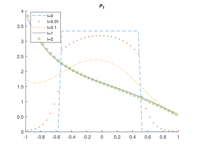
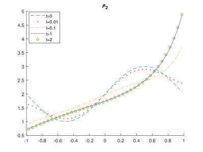
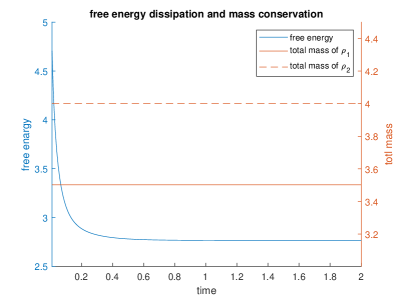
Example 5.2.
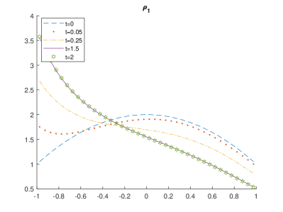
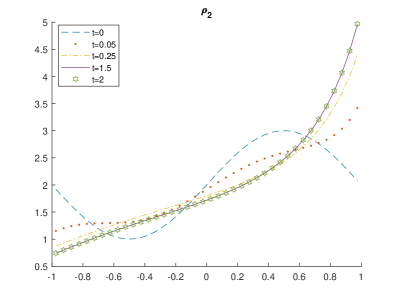
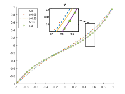
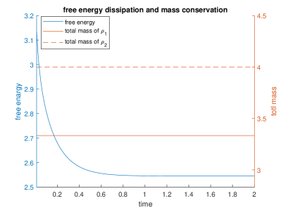
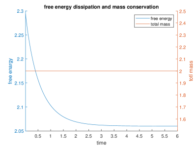
In this test, still with the initial boundary value problem (5.1)-(5.2), we show the proven solution properties. We take to compute the numerical solutions up to . Solutions at are given in Figure 1. In Figure 2 are total mass of and , and free energy profile. We see from Figure 1 and Figure 2 that the scheme is positivity preserving, mass conservative, and energy dissipating.
Example 5.3.
(Positivity propagation) In this test, we consider the PNP system (5.1) with following initial and boundary conditions
| (5.3) | ||||
We take to compute the numerical solutions up to . Solutions at are displayed in Figure 3. In Figure 4 are total mass of , , and free energy profile. From these results we see that the scheme is positivity preserving, mass conservative, and energy dissipating. We also observe that steady state solutions are identical to those in Example 5.2; this suggests that steady state solutions of the PNP systems with Dirichlet boundary condition only depends on the total mass and the Dirichlet boundary condition, but not sensitive to the profile of the initial data.
In Table 3 we compare CPU times (in seconds) for the PDIP method and the PG method. Here we set and choose different number of sub-intervals.
| h | 1/10 | 1/50 | 1/100 | 1/150 | 1/200 | 1/20 | 1/300 |
|---|---|---|---|---|---|---|---|
| PDIP | 1.22 | 2.37 | 8.38 | 17.73 | 31.32 | 48.97 | 74.71 |
| PG | 0.19 | 0.39 | 1.15 | 2.02 | 3.12 | 4.56 | 6.38 |
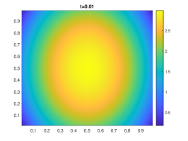
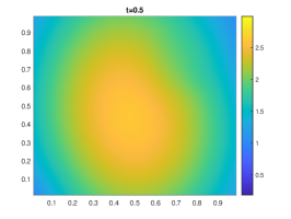
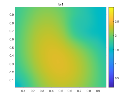
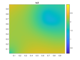
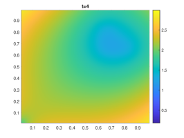
Example 5.4.
2D single species (Neumann boundary condition). We now apply our scheme to solve the 2D single-species PNP system
on domain . We consider the initial boundary conditions
The permanent charge is
| (5.4) |
This problem satisfies the compatibility condition (2.4). We take to compute the numerical solutions up to . Color plot of the solutions at are given in Figure 5. In Figure 6 are total mass of and free energy profile

6. Concluding remarks
In this paper, a dynamic mass transport method for the PNP system is established by drawing ideas from both the JKO-type scheme [19, 20] and the classical Bennamou-Breiner formulation [3]. The energy estimate resembles the physical energy law that governs the PNP system in the continuous case, where the JKO type formulation is an essential component for preserving intrinsic solution properties. Both mass conservation and the energy stability are shown to hold, irrespective of the size of time steps. To reduce computational cost, we use a local approximation for the artificial time in the constraint transport equation by a one step difference and the integral in time by a one term quadrature.
Furthermore, by imposing a centered finite difference discretization in spatial variables, we establish the solvability of the constrained optimization problem. This also leads to a remarkable result: for any fixed time step and spatial meth size, density positivity will be propagating over all time steps, which is desired for any discrete version of the PNP system.
In the previous section, some numerical experiments were carried out to demonstrate the proven properties of a computed solution. The first experiment numerically verified that the variational scheme yields convergence to the solution of the nonlinear PDE with desired accuracy. Secondly, with further examples the computed solutions are also shown to satisfy the energy law for the PNP system, mass conservation, and positivity propagation. It is a matter of future work to prove an error estimate for these numerical solutions. This is not a standard error analysis due to the nonlinearities in these problems, as well as the reformulation as a constrained optimization problem.
Acknowledgments
This research was partially supported by the National Science Foundation under Grant DMS1812666.
References
- [1] L. Ambrosio, N. Gigli, and G. Savaré. Gradient flows in metric spaces and in the space of probability measures. Lect. Math., ETH Zürich. Birkhäuser Verlag, Basel., 2005.
- [2] M.Z. Bazant, K. Thornton, and A. Ajdari. Diffuse-charge dynamics in electrochemical systems. Phys. Rev. E., 70: 021506, 2004.
- [3] J.-D. Benamou and Y. Brenier. A computational fluid mechanics solution to the Monge-Kantorovich mass transfer problem. Numer. Math., 84: 375–393, 2000.
- [4] M. Burger, B. Schlake, and M.-T. Wolfram. Nonlinear Poisson-Nernst-Planck equations for ion flux through confined geometries. Nonlinearity., 25: 961–990, 2012.
- [5] J. A. Carrillo, K. Craig, L. Wang, and C. Wei. Primal dual methods for Wasserstein gradient flows. Found. Comput. Math., 22:389–443, 2022.
- [6] D. Chen and R. Eisenberg. Poisson-Nernst-Planck (PNP) theory of open ionic channels. Biophys. J., 64: A22, 1993.
- [7] J. Ding, Z. Wang, and S. Zhou. Positivity preserving finite difference methods for Poisson-Nernst-Planck equations with steric interactions: Application to slit-shaped nanopore conductance. J. Comput. Phys., 397: 108864, 2019.
- [8] J. Ding, C. Wang, and S. Zhou. Convergence analysis of structure-preserving numerical methods based on Slotboom transformation for the Poisson–Nernst–Planck equations. arXiv:2202.10931, 2022.
- [9] B. Eisenberg. Ionic channels in biological membranes - electrostatic analysis of a natural nanotube. Contemp. Phys., 39 (6): 447–466, 1998.
- [10] A. Flavell, M. Machen, R. Eisenberg, J. Kabre, C. Liu, and X. Li. A conservative finite difference scheme for Poisson-Nernst-Planck equations. J. Comput. Electron., 15: 1–15, 2013.
- [11] A. Flavell, J. Kabre, and X. Li. An energy-preserving discretization for the Poisson-Nernst-Planck equations. J. Comput. Electron., 16: 431–441, 2017.
- [12] H. Gao and D. He. Linearized conservative finite element methods for the Nernst-Planck-Poisson equations. J. Sci. Comput., 72: 1269–1289, 2017.
- [13] D. He and K. Pan. An energy preserving finite difference scheme for the Poisson-Nernst-Planck system. Appl. Math. Comput., 287: 214–223, 2016.
- [14] D. He, K. Pan, and X. Yue. A positivity preserving and free energy dissipative difference scheme for the Poisson-Nernst-Planck system. J. Sci. Comput., 81: 436–458, 2019.
- [15] J.W. Hu and X.D. Huang. A fully discrete positivity-preserving and energy-dissipative finite difference scheme for Poisson-Nernst-Planck equations Numer. Math., 145: 77–115, 2020.
- [16] X. Huo, H. Liu, A. E. Tzavaras, and S. Wang. An Energy Stable and Positivity-Preserving Scheme for the Maxwell-Stefan Diffusion System. SIAM J. Numer. Anal., 59(5): 2321–2345, 2021.
- [17] J.W. Jerome. Consistency of semiconductor modeling: an existence/stability analysis for the sationary Van Roosbroeck system. SIAM J. Appl. Math., 45 (4): 565–590, 1985.
- [18] S. Ji and W. Liu. Poisson-Nernst-Planck systems for ion flow with density functional theory for hard-sphere potential: I-V relations and critical potentials. Part I: analysis. J. Dyn. Diff. Equat., 24: 955–983, 2012.
- [19] R. Jordan, D. Kinderlehrer, and F. Otto. The variational formulation of the Fokker- Plank equation. SIAM. J. Math. Anal., 29(1):1–17, 1998.
- [20] D. Kinderlehrer, L. Monsaingeon, and X. Xu. A Wasserstein gradient flow approach to Poisson-Nernst-Planck equations. ESAIM: Control Optim. Calc. Var., 23(1):137–164, 2017.
- [21] H. Liu and W. Maimaitiyiming. Energy stable and unconditional positive schemes for a reduced Poisson-Nernst- Plank system. Comm. Comput. Phys., 7(5): 1505–1529, 2020.
- [22] H. Liu and W. Maimaitiyiming. Efficient, positive, and energy stable schemes for multi-D Poisson–Nernst–Planck Systems. J. of Sci Comput, 87(3):1–36, 2021.
- [23] H. Liu and Z. Wang. A free energy satisfying finite difference method for Poisson-Nernst-Planck equations. J. Comput. Phys., 268: 363–376, 2014.
- [24] H. Liu and Z. Wang. A free energy satisfying discontinues Galerkin method for one-dimensional Poisson-Nernst-Planck systems. J. Comput. Phys., 328: 413–437, 2017.
- [25] H. Liu, Z. Wang, P. Yin, and H. Yu. Positivity-preserving third order DG schemes for Poisson–Nernst–Planck equations. J. Comput. Phys., 452: 110777, 2022.
- [26] W.-C. Li, J.-F. Lu, and L. Wang. Fisher information regularization schemes for Wasserstein gradient flows. J. Comput. Phys., 416:109449, 2020.
- [27] W. Liu. Geometric singular perturbation approach to steady state Poisson-Nernst-Planck systems. SIAM J. Appl. Math., 65 (3): 754–766, 2005.
- [28] C. Liu, C. Wang, S. M. Wise, X. Yue, and S. Zhou. A positivity-preserving, energy stable and convergent numerical scheme for the Poisson-Nernst-Planck system. Math. Comp., 90(331), 2071–2106, 2021.
- [29] P.A. Markowich, C.A. Ringhofer, and C. Schmeiser. Semiconductor Equations. Springer- Verlag, 1990.
- [30] D. Matthes and S. Plazotta. A variational formulation of the BDF2 method for metric gradient flows. ESAIM: M2AN, 53: 145–172, 2019 .
- [31] M.S. Metti, J. Xu, and C. Liu. Energetically stable discretizations for charge transport and electrokinetic models. J. Comput. Phys., 306: 1–18, 2016 .
- [32] J. Nocedal, S. J. Wright. Numerical Optimization. Springer, 2006.
- [33] J.-H. Park and J. Jerome. Qualitative properties of steady-state Poisson-Nernst-Planck systems: Mathematical study. SIAM J. Appl. Math., 57 (3): 609–630, 1997.
- [34] S. Selberherr. Analysis and Simulation of Semiconductor Devices. Springer-Verlag/Wien,New York, 1984.
- [35] J. Shen, J. Xu. Unconditionally positivity preserving and energy dissipative schemes for Poisson-Nernst-Planck equations. Numer. Math., 148(3): 671–697, 2021.
- [36] R. Shen, Q. Zhang, ang B. Lu. An inverse averaging finite element method for solving the size-modified Poisson-Nernst-Planck equations in ion channel simulations. arXiv:2112.01692, 2021.
- [37] T. Teorell. Transport processes and electrical phenomena in ionic membranes. Progress Biophysics, 3: 305, 1953.