Water wave problem with inclined walls

Abstract

We study free surface water waves in a 2-D symmetric triangular channel with sides that have a $45^{o}$ slope. We develop models for small amplitude nonlinear waves, extending earlier studies that have considered the linearized problem. We see that a combination of heuristic small amplitude expansions lead to a relatively simple system that we then use to study interactions of low frequency modes. The formalism relies on an explicit construction of the normal modes of the linear problem and a new way to represent the free surface. We argue that the construction can be applied to more general geometries. We also examine the structure and some dynamical features of spectral truncations for the lowest even modes.

Keywords: gravity water waves; free surface potential flow; fluid domains with slopping walls; low Mode interactions in a triangular domain; wave run-up.

1 Introduction

We propose a simplified nonlinear model for free surface potential flow in 2-D domains with slopping lateral rigid wall boundaries. i.e. “beach geometries”. The paper is partially motivated by classical studies of the linearized system, especially works on special geometries where the linear normal modes can be found in explicit or semi-explicit ways, such as isosceles triangles with sides inclined at $45^{o}$ and $60^{o}$ to the vertical, see [K79, KH80, G87, M93, L32, P80, G94, G95, VMMP19], and semicircular channels [EL93]. The theory extends to 3-D channels with constant cross sections given by the above shapes [M93, G94, G95]. The suitability of the potential flow model for problems in such geometries may be questioned on physical grounds, and there are alternative models currently in use that incorporate other effects, see e.g. [HN81, LL89, KMT91, BB08, TFPP13]. On the other hand the potential flow theory has made considerable advances into the related problem of waves in variable depth [CGNS05, L13, AP17, AN18], and the present work considers some of the geometrical problems involved in approximating the potential flow system in inclined wall geometries. Our main goal is to obtain a simple weakly nonlinear model that can be also generalized to other geometries. Our strategy is to work almost exclusively with the $45^{o}$ isosceles triangle domain [K79, KH80, G87, L32]. We see that the derivation of a weakly nonlinear system points to possible extensions to more general domains, although workable models for general domains involve nontrivial additional ingredients that are left for future work.

The main feature of our approach is a new description of the free surface as the image of the flat surface under the flow of a vector field that is the gradient of a harmonic function with vanishing normal derivative at the rigid walls. The dynamical variables of the problem are then the usual velocity potential, and this second harmonic function used to compute the free surface. We show that this description of the system, together with the Euler equations for potential flow, can be used to derive a simpler approximate model equation for weakly nonlinear waves. The derivation also relies on an explicit small amplitude approximation of the free surface and uses expansions in the normal modes of the linear problem. The goal of the paper is to show how this formulation can be used to compute dynamical quantities of special interest such as wave run-up on a beach.

The proposed representation of the free surface is motivated by limitations of the simpler graph description in domains with inclined domains and is described in section 2, where we also discuss its main properties, advantages, and disadvantages. Our definition implies that the free surface satisfies automatically some desirable geometrical properties, such as area conservation, and non self-intersection. Also, the end points of the free surface are always on the rigid wall. Such properties should follow from the dynamics of the fluid, but are here imposed by the representation of the free surface. This allows for more drastic approximations of the dynamical equations. A drawback of the proposed representation is that in general there is no explicit exact expression of the free surface in terms of the auxiliary potential. Despite this fact, the existence and properties of the curve representing free surface can be deduced using basic facts from the theory of ordinary differential equations, see e.g. [P91]. Most importantly, the free surface can be expressed explicitly in terms of the auxiliary potential using approximate formulas that can be interpreted as small amplitude (surface deformation) expansions. We show that the geometrical properties of the exact curves are also satisfied by such approximations, either exactly or approximately, with errors that we can quantify. We also point out a simple approximation, related to Euler’s formula for numerical integration, that is especially useful for domains with constant slope.

We then show that the proposed description of the free surface, its small deformation approximation by Euler’s formula, and the equations for free surface potential flow can be combined to derive an approximate equation for weakly nonlinear waves. The first step of this derivation leads to the linear evolution equations appearing in the classical results on normal modes cited above. The results on the linear problem are then used to derive a lowest order (quadratic) nonlinear model for the interactions of the normal modes of the linearized problem. The construction of the spectral equation uses the results of [K79, KH80, G87, L32] on linear normal modes of the $45^{o}$ triangular domain. The normal modes form a set of functions that are harmonic in the domain that can be occupied by the fluid and also satisfy the rigid wall boundary conditions. Similar functions are known in simpler geometries, e.g. the constant depth channel, and are also used in the computation of the Dirichlet-Neumann operator and the derivation of approximate models [CS93], see also [WV15] for comparison of different methods. The paper shows that the tools used to analyze the Dirichlet-Neumann operator can be used to describe the free surface in domains with inclined walls.

We also argue that the derivation of the nonlinear model equation can be meaningful for general domains with slopping beaches. This equation is potentially interesting for its structure, but in the absence of explicit expressions for the normal modes its numerical study will require alternative discretizations. The model also involves the Dirichlet-Neumann operator for the flat surface domain and related regularity questions that require some care [MW16]. These questions are more tractable in the special geometry we consider as we work with linear combinations of functions that are harmonic in domains that include the fluid domain. We note that quadratic water wave models with full dispersion (e.g. “Whitham-Boussinesq” systems) [AMP13, MKD15, H17, HT18] can capture several effects of more involved models see e.g. [VP16, C18, VMS21], especially in the long wave regime.

We apply the quadratic model to study mode interactions in the $45^{o}$ triangular domain. We examine the evolution on the invariant subspace of even modes and present numerical experiments of nonlinear mode interactions, and the computation of the corresponding wave amplitudes and run-up. We focus on near-monochromatic initial conditions, and we gradually increase the amplitude to see nonlinear mode interactions leading to amplitude and phase modulation of the dominant mode. Some solutions with two modes of comparable amplitude are also presented. In all cases larger initial conditions lead to rapid growth of the amplitude and we focus on results suggesting long time existence for small amplitudes. Nonlinear mode interactions lead to marked effects on wave run-up at the beach. The long time dynamics of the truncated mode interactions can be examined in more detail in future work and we comment on some relevant issues in the discussion section. The construction of the mode interaction systems involves the computation of mode interaction coefficients, details are presented in a Supplement.

In section 2 we present the general formalism, the derivation of an approximate model for the $45^{o}$ domain and discuss generalizations. In section 3 we present some computations with the quadratic spectral equations on the invariant space of even modes. In section 4 we discuss some limitations of the present study and possible further work. Computations of mode interaction coefficients are detailed in a Supplement.

2 Free surface formulation and weakly nonlinear model

In this section we introduce the description of the free surface by a potential in its exact and approximate form. We use the equations of free surface potential flow to show how this description leads to the well known problem of linear modes. We further use the approximate description of the free surface and the analysis of the linearized problem to derive an approximate weakly nonlinear model and write it in spectral form. We discuss generalizations and further properties and limitations of the proposed description of the free surface.

We consider free surface potential flow in two dimensional domain with rigid walls at

$$\partial{\cal W}=\{[x,y]\in\mathbb{R}^{2}:y=|x|\}.$$ (2.1)

The fluid will occupy a time-dependent domain $D_{t}$ contained in the set ${\cal W}=\{[x,y]\in\mathbb{R}^{2}:y\geq|x|\}$. The fluid surface at rest is at $y=B>0$.

The free surface at time $t$ can be parametrized by a curve $[X(s,t),Y(s,t)]$, $s\in[-h,h]$. Such a curve is assumed to not self-intersect, to intersect the boundary $\partial{\cal W}$ only at $s=\pm h$, and to satisfy boundary conditions $-X(-h,t)=Y(-h,t)$ and $X(h,t)=Y(h,t)$. By conservation of fluid volume it should also satisfy

$$\frac{1}{2}\int_{-h}^{h}(Y(s,t)\;dX-X(s,t)\;dY)=B^{2}.$$ (2.2)

We expect that the evolution preserves these conditions.

2.1 Description of the free surface

We propose a more restricted but less explicit way to parametrize the free surface as

$$[X(s,t),Y(s,t)]={\cal G}^{\epsilon}(s,t)\in\mathbb{R}^{2},\quad s\in[-h,h],$$ (2.3)

$\epsilon>0$ a constant, where ${\cal G}^{\epsilon}(s,t)$ is the image of the set $\{[x,y]\in\mathbb{R}^{2}:x\in[-h,h],y=B\}$, the free surface at rest, under the “time$-\epsilon$ flow” (see next paragraph for this terminology) of a vector field of the form $\nabla V(\cdot,t)$ in ${\cal W}$ with $V(\cdot,t)$ a function that is harmonic in ${\cal W}$ and satisfies the Neumann condition ${\hat{n}}\cdot\nabla V(\cdot,t)=0$ at $\partial{\cal W}$, $\hat{n}$ the normal vector at $\partial{\cal W}$, for all times $t$.

The above definition uses some basic facts and terminology from the theory of ordinary differential equations, and we provide some additional details. Specifically, for each time $t$, fix $t$ and consider the ordinary differential equation

$$\frac{dr}{d\tau}=\nabla V(r,t),\quad r\in{\cal W}.$$ (2.4)

The variable $\tau$ is not the physical time but rather the variable used to parametrize the integral curves of the vector field $\nabla V(\cdot,t)$ at each fixed time $t$, also $r=[x,y]$ are coordinates of points in $\cal W$. To construct ${\cal G}^{\epsilon}(\cdot,t)$ we integrate (2.4) in $\tau$, then ${\cal G}^{\epsilon}(s,t)$ is the unique solution $r(\tau,s;t)$ of (2.4) at $\tau=\epsilon$ that satisfies $r(\tau)=[s,B]$ at $\tau=0$. (The “time$-\epsilon$ map” of (2.4) is the map from the $r(0)=[s,B]$ to the $r(\epsilon,s;t)$, with $s\in[-h,h]$.) The existence and uniqueness of such $r(\tau,s;t)$ for all $s\in[-h,h]$ at any given $t$ follows from the theory of existence and uniqueness for ordinary differential equations under certain (continuity, differentiabilty, etc.) assumptions on the vector field $\nabla V(\cdot,t)$, see e.g. [P91], ch. 2, and [L07], ch. 5. We assume that these conditions are satisfied for all $t$. This can be checked once we have $V(\cdot,t)$, see Remark 2.1 for some details. Figure 1 shows a schematic diagram of map ${\cal G}^{\epsilon}(s,t)$ at time $t$ with $s\in[-h,h].$

Thus the dynamical variable behind this representation the free surface is $V(\cdot,t)$, i.e. $V(\cdot,t)$ determines ${\cal G}^{\epsilon}(s,t)$ uniquely, for all $s\in[-h,h]$ and $t$. The dynamical equation for $V$ are derived in the next subsections. Note that the definition of ${\cal G}^{\epsilon}(\cdot,t)$ is abstract, in that we do not have an explicit expression for ${\cal G}^{\epsilon}(\cdot,t)$ in terms of $V(\cdot,t)$. We emphasize however that for $\epsilon$ small, the solution of (2.4) can be approximated by explicit formulas, i.e. expressions that are given in terms of $V$. (Such formulas are used in numerical integrators, see e.g. [L07].) One such approximation, Euler’s formula, is defined in subsection 2.4 below, and used in the derivation of approximate equations for $V$ in subsections 2.5-2.7.

The representation of the free surface by ${\cal G}^{\epsilon}$ implies that the curve representing the free surface satisfies a number of desirable properties. First, (2.3), (2.4) imply area conservation, and (2.2), at all times $t$. This follows by $V$ harmonic in ${\cal W}$, then the divergence of $\nabla V$ vanishes, and we have volume conservation by a standard argument, see also [P91], ch. 2. Furthermore, ${\cal G}^{\epsilon}$ maps the points $s=\pm h$ to points on $\partial{\cal W}$ at all times $t$, i.e. these two points are always on the wall. This follows from the fact that $\nabla V$ is tangent to $\partial{\cal W}$, at all times. Then the integral curves of (2.4) passing from any point on $\partial{\cal W}$ stay on $\partial{\cal W}$. Note that ${\cal G}^{\epsilon}(\pm h,t)$ are the points where the free surface intersects the rigid wall. We also check that these are the only points where the free surface ${\cal G}^{\epsilon}(s,t)$, $s\in[-h,h]$, can intersect the rigid wall: any point of ${\cal G}^{\epsilon}(s_{*},t)$, $s\in(-h,h)$, in $\partial{\cal W}$, must satisfy ${\cal G}^{0}(s_{*},t)=s_{*}\in\partial{\cal W}$ by the invariance of $\partial{\cal W}$ under the flow of $\nabla V(\cdot,t)$. That would imply $s_{*}\in\{-h,h\}$, a contradiction. Also, by the theory of existence and uniqueness of the initial value problem for (2.4), the function $[s,B]\mapsto{\cal G}^{\epsilon}(s,t)$, $s\in[-h,h]$, defining the free surface is invertible [P91]. This fact implies that the free surface can not self-intersect, i.e. there are no $-h<s_{1}<s_{2}<h$ and $t$ for which ${\cal G}^{\epsilon}(s_{1},t)={\cal G}^{\epsilon}(s_{2},t)$.

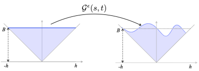
Figure 1: The free surface at time $t$ is represented by a map ${\cal G}^{\epsilon}(s,t)$, $s\in[-h,h]$, of the blue line on the left to the blue curve on the right. ${\cal G}^{\epsilon}$ is constructed by fixing $t$ and integrating (2.4) in $\tau$ from $\tau=0$ to $\tau=\epsilon$ with initial conditions the points on the blue curve on the left (the flat surface). The map ${\cal G}^{\epsilon}$ can be approximated by explicit expressions.

The proposed description of the free surface is motivated by the difficulty in using the usual simpler definition of the free surface as a graph, i.e. as the set of points with cartesian coordinates $[x,\eta(x,t)]$. The problem in a fluid domain with inclined walls is that the domain of the horizontal coordinate $x$ will generally vary in time. Many works, including the cited literature on linear normal modes, do not address this issue, but still obtain meaningful results, see e.g. [L32]. However the point where the free surface intersects the rigid wall is defined in an ad-hoc way, e.g. the normal mode equation is defined for $x$ is in a fixed domain, the free surface at rest, and the domain of $\eta$ is extended to a larger set. This allows us to determine the intersection of the graph of this extended $\eta$ and the rigid wall. More importantly, the absence of a clear definition of the free surface in the classical linear literature is an obstacle to deriving weakly nonlinear equations.

The use of systems of coordinates where the rigid wall is the vertical direction is possible, but this approach requires different systems for each domain. Also the height of fluid at rest is not constant. The work of [C17] discusses more general parametrizations in two dimensions that can be also used for domains with inclined walls, especially parametrization by arc length. These parametrizations do not satisfy automatically the geometrical properties of ${\cal G^{\epsilon}}$ discussed above, e.g. area conservation and permanence of the end points on the wall relies on the dynamics. The proposed method can be also applied to three dimensional domains, e.g. using the classical normal mode results for some three dimensional channels with constant cross section [G94, G95]. An alternative more general description of the free surface that uses level sets has been implemented numerically and used extensively in coastal engineering, using Navier-Stokes (and versions with turbulent Reynolds stress terms) [HN81, LL89, KMT91, BB08, TFPP13]. These equations can not be reduced to equations for surface quantities. Independently of this fact, the level set approach is more complicated as it adds a partial differential equation for the evolution of the fluid domain, and may not easily lead to the kind of more quantitative analysis that seems possible with our model. Further comments on the advantages and disadvantages of the proposed description of the free surface at the end of this section, and in the discussion section.

We now discuss the dynamics of the free surface system. We show that we can combine the description of the free surface above, an approximation of ${\cal G}^{\epsilon}$ defined below, and the equations of motion for free surface potential flow to obtain approximate equations for the evolution of the free surface and the velocity inside the fluid.

2.2 Dynamical variables of the system

A preliminary step is to identify the dynamical variables of the problem. These will be the potential $V(\cdot,t)$ used to define the free surface via (2.4), and the hydrodynamic potential $\phi(\cdot,t)$. Both quantities will be also represented by an expansion in a set of harmonic functions $\Phi_{n}$ that will be given explicitly below. They appear in the analysis of the linearized system below.

First, the set of possible harmonic functions $V(\cdot,t)$ will be written as

$$V(\cdot,t)=\sum_{n=1}^{\infty}b_{n}(t)\Phi_{n}(\cdot),$$ (2.5)

where the functions $\Phi_{n}$, to be specified below, are harmonic in ${\cal W}$ and satisfy $\partial_{\hat{n}}\Phi_{n}=0$ at $\partial{\cal W}$.

In free surface potential flow, the Eulerian velocity $u$ in the fluid domain will be $u=\nabla\phi$, with $\phi$ harmonic in $\cal W$ with vanishing normal derivative at $\partial{\cal W}$. We will expand $\phi(\cdot,t)$ as

$$\phi(\cdot,t)=\sum_{n=1}^{\infty}a_{n}(t)\Phi_{n}(\cdot).$$ (2.6)

By the properties of the $\Phi_{n}$, $\phi(\cdot,t)$ is harmonic in ${\cal W}$ and satisfies $\partial_{\hat{n}}\phi=0$ at $\partial{\cal W}$.

Remark 2.1

(i) One of the ideas implicit on the above expansions is that the descriptions of $V$ (hence the free surface), and $\phi$ involve similar tools. (ii) We see below that the functions $\Phi_{n}$ used in the $45^{0}$ slope domain are analytic on the whole plain. The properties of $V$ needed to guarantee the existence of ${\cal G}^{\epsilon}$, e.g. the size of the derivative of $\nabla V$ in a neighborhood of the triangle bounded by $\cal W$ and points with height $y<B$, see e.g. [L07], ch. 5, are controlled by the size of the $b_{n}$. The nontrivial information is the evolution of the $b_{n}$. Truncations to finite sums used in the next section again make these technicalities much more tractable as long at the $b_{n}$ remain bounded.

To derive equations for the evolution of $V$, $\phi$ we use Euler’s equations for free surface potential flow.

2.3 Equations of motion

In what follows we denote the horizontal and vertical components of ${\cal G}^{\epsilon}$ by ${\cal G}_{1}^{\epsilon}$, ${\cal G}_{2}^{\epsilon}$ respectively.

Then the equations of motion for gravity water waves are

$$\partial_{t}{\cal G}^{\epsilon}(s,t)=\nabla\phi\left({\cal G}^{\epsilon}(s,t),t\right),$$ (2.7)

$$\partial_{t}\phi(z,t)+\frac{1}{2}|\nabla\phi(z,t)|^{2}+g(y-B)=0,\quad\hbox{at}\quad z=[x,y]={\cal G}^{\epsilon}(s,t),\quad s\in[-h,h].$$ (2.8)

The first equation states that the free surface is transported by the flow. The second equation is the Bernoulli equation at the free surface, assuming a constant vertical gravitational field of magnitude $g$ and vanishing pressure at the surface.

The general idea is that (2.7), (2.8) should imply an evolution equation for the variables $V$, $\phi$, equivalently the coefficients $a_{n}$, $b_{n}$ above. This is not obvious since $V$ appears implicitly in equations (2.7), (2.8). To obtain these evolution equations we use a small amplitude approximation of ${\cal G}^{\epsilon}$ in terms of $V$. The $\Phi_{n}$ will be determined in the process.

2.4 Explicit approximate representations of the free surface

The free surface ${\cal G}^{\epsilon}$ can be approximated by its Taylor series at $\epsilon=0$, under standard regularity assumptions on $\nabla V$. In what follows we will use the lowest order nontrivial approximation

$${\cal G}^{\epsilon}(s,t)=[s,B]+\epsilon[\partial_{x}V([s,B],t),\partial_{y}V([s,B],t)]+O(\epsilon^{2}).$$ (2.9)

Truncating to $O(\epsilon^{2})$ we have approximate integration of (2.4) by Euler’s rule. We denote this approximation by ${\cal G}^{\epsilon}_{E}$, and we have

$${\cal G}^{\epsilon}_{E}(s,t) = [s+\epsilon\partial_{x}V([s,B],t),B+\epsilon\partial_{y}V([s,B],t)]$$ (2.10)

$$= [s+\epsilon\sum_{n=1}^{\infty}b_{n}(t)\partial_{x}\Phi_{n}([s,B]),B+\epsilon\sum_{n=1}^{\infty}b_{n}(t)\partial_{y}\Phi_{n}([s,B])],$$ (2.11)

by (2.5).

We may interpret ${\cal G}^{\epsilon}_{E}$ as a small amplitude approximation of ${\cal G}^{\epsilon}$. By the assumption ${\hat{n}}\cdot{\nabla V}(\cdot,t)=0$ at $\partial W$, $\nabla V$ at the endpoints $[\pm h,B]$ is parallel to the boundary, and the points $[\pm h,B]$ are mapped to points in $\partial W$ by ${\cal G}^{\epsilon}_{E}$. The approximation of the surface by Euler’s rule is therefore quite appropriate for inclined walls of constant slope (assuming that the triple interface moves in the regions of constant slope at all times). On the other hand, ${\cal G}^{\epsilon}_{E}$ preserves volume automatically, i.e. independently of the dynamics, up to $O(\epsilon^{2})$, see Proposition 2.5 and the discussion at the end of this section.

As an example of the use of this approximation for ${\cal G}^{\epsilon}$, the velocity at the free surface is

$$\nabla\phi\left({\cal G}^{\epsilon}(s,t),t\right)=\sum_{n=1}^{\infty}a_{n}(t)[\partial_{x}\Phi_{n}\left({\cal G}^{\epsilon}(s,t),t\right),\partial_{y}\Phi_{n}\left({\cal G}^{\epsilon}(s,t),t\right)]$$ (2.12)

by (2.6). By (2.9) we have to lowest order

$$\nabla\phi\left({\cal G}^{\epsilon}(s,t),t\right)=\nabla\phi\left([s,B]+O(\epsilon)\right)=\nabla\phi([s,B],t)+O(\epsilon).$$ (2.13)

The derivation of approximate models for the dynamical variables proceeds in two steps. In the first step we show that the lowest order approximations for ${\cal G}^{\epsilon}$ and $\phi$, and a scaling argument, lead to the well-known linear system for inclined wall domains.

2.5 Derivation and analysis of linearized system

We shall use ${\cal G}^{\epsilon}={\cal G}^{\epsilon}_{E}$, and $\phi=\epsilon{\tilde{\phi}}$. Then (2.7) becomes

$$\epsilon\partial_{t}[\partial_{x}V([s,B],t),\partial_{y}V([s,B],t)]=\epsilon[\partial_{x}{\tilde{\phi}}([s,B],t),\partial_{y}{\tilde{\phi}}([s,B],t)]+O(\epsilon^{2}),$$ (2.14)

while (2.8) becomes

$$\epsilon\partial_{t}{\tilde{\phi}}([s,B],t)+g\epsilon\partial_{y}V([s,B],t)+O(\epsilon^{2})=0,$$ (2.15)

i.e. the nonlinear part is $O(\epsilon^{2})$. To $O(\epsilon^{2})$, the second component of the first equation and the second equation lead to

$$\partial_{tt}{\tilde{\phi}}([s,B],t)+g\partial_{y}{\tilde{\phi}}([s,B],t)=0.$$ (2.16)

Equation (2.16), and

$$\Delta{\tilde{\phi}}=0\quad\hbox{in}\quad{\cal W},\quad{\hat{n}}\cdot{\tilde{\phi}}=0\quad\hbox{at}\quad\partial{\cal W},$$ (2.17)

form a linear evolution system for ${\tilde{\phi}}$. The first component of (2.14) can be used to obtain $V([s,B],t)$ from $\phi([s,B],t)$, and determine the free surface.

The $\Phi_{n}$ will be the normal modes of the linearized problem for $\tilde{\phi}$, that is solutions of (2.16), (2.17) of the form

$${\tilde{\phi}}([x,y],t)=\psi([x,y])e^{i\omega t}.$$ (2.18)

Then $\psi$ must satisfy

$$\omega^{2}\psi([s,B],t)=g\partial_{y}\psi([s,B],t),$$ (2.19)

and

$$\Delta{\psi}=0\quad\hbox{in}\quad{\cal W},\quad{\hat{n}}\cdot\nabla\psi=0\quad\hbox{at}\quad\partial{\cal W}.$$ (2.20)

Semi-explicit solutions were obtained by Kirchhoff [K79], see also Lamb [L32], Art. 261. We summarize the results.

The symmetric modes are $\psi=\Psi_{S}$, where

$$\Psi_{S}(x,y;\alpha)={\cal C}_{S}(\alpha)[\cosh(\alpha x)\cos(\alpha y)+\cos(\alpha x)\cosh(\alpha y)],$$ (2.21)

with ${\cal C}_{S}(\alpha)$ an arbitrary real. The $\Psi_{S}$ are harmonic in $\mathbb{R}^{2}$, satisfy the Neumann boundary condition at $\partial{\cal W}$, and are even in $x$, $\forall y\in\mathbb{R}$, for all real $\alpha$. By (2.19) $\alpha$ must satisfy

$$\tanh(\alpha B)=-\tan(\alpha B),$$ (2.22)

and $\omega=\omega(\alpha)$ are given by

$$\omega^{2}=g\alpha\tanh(\alpha B).$$ (2.23)

The antisymmetric modes are $\psi=\Psi_{A}$, where

$$\Psi_{A}(x,y;\alpha)={\cal C}_{A}(\alpha)[\sinh(\alpha x)\sin(\alpha y)+\sin(\alpha x)\sinh(\alpha y)],$$ (2.24)

with ${\cal C}_{A}$ an arbitrary real. The $\Psi_{A}$ are harmonic in $\mathbb{R}^{2}$, satisfy the Neumann boundary condition at $\partial{\cal W}$, and are odd in $x$, $\forall y\in\mathbb{R}$, for all real $\alpha$. By (2.19) $\alpha$ must satisfy

$$\tanh(\alpha B)=\tan(\alpha B),$$ (2.25)

and $\omega=\omega(\alpha)$ are given by

$$\omega^{2}=g\alpha\coth(\alpha B).$$ (2.26)

The constants ${\cal C}_{S}(\alpha)$, ${\cal C}_{A}(\alpha_{n})$ are arbitrary, they will be chosen below to normalize the modes.

There is an additional antisymmetric solution of (2.19), see [K79, L32], that does have the form (2.24), and that we denote by $\Phi_{1}$, it is given by

$$\Phi_{1}(x,y)=\sqrt{\frac{3}{2\pi^{5}}}xy.$$ (2.27)

By (2.19) the corresponding frequency $\omega_{1}$ is given by $\omega^{2}_{1}=g/B$. We do not consider the zero eigenvalue of (2.19), it corresponds to the constant harmonic function and does not contribute to the expansions for $V$, $\phi$.

The solutions of (2.23) (even mode wavenumbers) are denoted by $\alpha_{2j+2}$, $j\in\mathbb{N}\cup\{0\}$, and satisfy

$$\alpha_{2j+2}B\in(\pi/2+j\pi,\pi+j\pi),\quad j=0,1,2,\ldots.$$ (2.28)

In the limit $j\rightarrow\infty$ we have $\alpha_{2j+2}B\rightarrow j\pi+3\pi/4$, the solutions of $-\tan\alpha B=1$.

The solutions of (2.26) (odd mode wavenumbers) are denoted by $\alpha_{2k+1}$, $k\in\mathbb{Z}^{+}$, and satisfy

$$\alpha_{2k+1}B\in(k\pi,{\pi}/2+k\pi),\quad k=1,2,\ldots.$$ (2.29)

In the limit $k\rightarrow\infty$ we have $\alpha_{2k+1}B\rightarrow k\pi+\pi/4$, the solutions of $\tan\alpha B=1$.

Combining with (2.23), (2.26), the dispersion relation is

$$\omega^{2}_{1}=\frac{g}{B},\quad\omega_{n}^{2}=\begin{cases}g\alpha_{n}\tanh{\alpha}_{n}B,\quad n=2,4,6,\ldots;\\ g\alpha_{n}\coth{\alpha}_{n}B,\quad n=3,5,7,\ldots.\end{cases}$$ (2.30)

Proposition 2.2

The dispersion relation $\omega_{n}$, $n\in\mathbb{N}$ of (2.30) is strictly increasing.

A proof is given in the Appendix. We examine the dispersion relation in some more detail in the next section. The $\Phi_{n}$ of (2.5), (2.6) are then defined by

$$\Phi_{1}(x,y)=\Psi_{1}(x,y),\quad\Phi_{n}(x,y)=\begin{cases}\Psi_{S}(x,y;\alpha_{n}),\quad n=2,4,6,\ldots;\\ \Psi_{A}(x,y;\alpha_{n}),\quad n=3,5,7,\ldots.\end{cases}$$ (2.31)

We also let

$$\xi_{n}(x)=\Phi_{n}(x,B),\quad n\in\mathbb{N},$$ (2.32)

The real numbers ${\cal C}_{S}(\alpha)$, ${\cal C}_{A}(\alpha)$, defined for $\alpha=\alpha_{n}$, $n$ odd and even positive integers respectively are still arbitrary. We use the notation ${\cal C}_{S}(n)={\cal C}_{S}(\alpha_{n})$ for $n$ even, and ${\cal C}_{A}(n)={\cal C}_{A}(\alpha_{n})$ for $n\geq 3$ odd. In what follows we choose them so that $\int_{-h}^{h}|\xi_{n}|^{2}=1$, $\forall n\mathbb{N}$. $\xi_{1}$ is already normalized for $h=\pi$.

By (2.19), (2.20) the $\xi_{n}$ are eigenfunctions of the flat surface Dirichlet-Neumann operator ${\hat{\partial}}_{y}$, defined by

$${\hat{\partial}}_{y}\xi_{n}(s)=\partial_{y}\Phi_{n}(s,B)=g^{-1}\omega^{2}_{n}\Phi_{n}(s,B)=g^{-1}\omega^{2}_{n}\xi_{n}(s),$$ (2.33)

for all $s\in[-h,h]$, and $n\in\mathbb{Z}^{+}$.

Let $X=L^{2}([-h,h];\mathbb{R})$ with the standard inner product $\langle f,g\rangle=\int_{-h}^{h}f(s)g(s)\;ds$. The operator ${\hat{\partial}}_{y}$ is a symmetric operator in $X$ with dense domain, moreover the $\{\xi_{n}\}_{n=1}^{\infty}$ form a orthonormal set in $X$. Orthogonality follows by Proposition 2.2 and Green’s identity. Also, (2.33), $\omega_{n}\neq 0$, implies that the $\xi_{n}$ have zero average, $\forall n\geq 1$. Some related spectral theory is presented in [G94] for the related problem on channels with constant cross section.

2.6 Derivation of weakly nonlinear model

In the second step of deriving approximate equations for the dynamical variables we use the approximation of ${\cal G}^{\epsilon}$ by ${\cal G}^{\epsilon}_{E}$ to write an approximate evolution equation that includes the linearized equation above and a lowest order nonlinear part.

We use ${\cal G}^{\epsilon}={\cal G}^{\epsilon}_{E}$, ${\cal G}^{\epsilon}_{E}$ as in (2.10), and $\phi=\epsilon\psi$, then the first equation (2.7) is

$$\epsilon\partial_{t}\partial_{x}V([s,B],t) = \epsilon\partial_{x}\psi(s+\epsilon\partial_{x}V([s,B],t),B+\epsilon\partial_{y}V([s,B],t),t),$$ (2.34)

$$\epsilon\partial_{t}\partial_{y}V([s,B],t) = \epsilon\partial_{y}\psi(s+\epsilon\partial_{x}V([s,B],t),B+\epsilon\partial_{y}V([s,B],t),t).$$ (2.35)

Expanding the right-hand side we have

$$\partial_{t}\partial_{x}V([s,B],t) = \partial_{x}\psi([s,B],t)+\epsilon\Big{[}(\partial^{2}_{x}\psi([s,B],t))\partial_{x}V([s,B],t)+$$ (2.36)

$$+ (\partial_{y}\partial_{x}\psi([s,B],t))\partial_{y}V([s,B],t)\Big{]}+O(\epsilon^{2}),$$

$$\partial_{t}\partial_{y}V([s,B],t) = \partial_{y}\psi([s,B],t)+\epsilon\Big{[}(\partial_{x}\partial_{y}\psi([s,B],t))\partial_{x}V([s,B],t))+$$

$$+ (\partial^{2}_{y}\psi([s,B],t)))\partial_{y}V([s,B],t))\Big{]}+O(\epsilon^{2}).$$ (2.37)

The $\epsilon-$term can be abbreviated as $(\nabla V([s,B],t))\cdot\nabla\partial_{y}\psi([s,B],t)$.

Similarly, the Bernoulli equation (2.8) becomes

$$\epsilon\partial_{t}\psi([s,B] + \epsilon(\nabla\partial_{t}\psi([s,B],t)))\cdot\nabla V([s,B],t),t)+$$ (2.38)

$$+ \frac{1}{2}\epsilon^{2}|\nabla\psi([s,B]+\epsilon\nabla V([s,B],t),t)|^{2}+g\epsilon\partial_{y}V([s,B],t)=0,$$

therefore

$$\partial_{t}\psi([s,B],t) + g\partial_{y}V([s,B],t)+\epsilon\Big{[}\nabla\partial_{t}\psi([s,B],t))\cdot\nabla V([s,B],t)+$$ (2.39)

$$+ \frac{1}{2}|\nabla\psi([s,B],t)|^{2}\Big{]}=O(\epsilon^{2}).$$

The first approximate nonlinear model is obtained by omitting the $O(\epsilon^{2})$ terms in (2.36), (2.37), (2.39).

The dynamical variables are $\psi(\cdot,t)$ and $V(\cdot,t)$, equivalently the coefficients $a_{n}(t)$, $b_{n}(t)$, $n\in\mathbb{N}$, of (2.6), (2.5) respectively. To obtain the approximate evolution equations for $a_{n}$, $b_{n}$, we will consider a system of two equations, one of the approximate transport equations (2.36), (2.37), and the approximate Bernoulli (2.39).

Note that (2.39) is implicit for $\partial_{t}\psi$. We have a term

$$\partial_{t}\psi+\epsilon(\partial_{t}\nabla\psi)\cdot\nabla V=\sum_{n=1}^{\infty}{\dot{a}}_{n}(t)\left(\Phi_{n}(s,B)+\epsilon\nabla\Phi_{n}(s,B)\cdot\nabla V([s,B]),t)\right).$$ (2.40)

We also need to expand $\nabla V$, so that we will have sums of terms ${\dot{a}}_{n}b_{m}$, and we need to invert an operator to write the equation for the ${\dot{a}}_{n}$ and $\partial_{t}\psi$.

One way to avoid this complication is to write $\partial_{t}\nabla\psi=\nabla\partial_{t}\psi$, and use

$$\partial_{t}\psi([s,B],t)=-g\partial_{y}V([s,B],t)+O(\epsilon)$$

from (2.39). Then the approximate Bernoulli equation is, up to $O(\epsilon^{2})$,

$$\partial_{t}\psi([s,B],t) = -g\partial_{y}V([s,B],t)+$$ (2.41)

$$+ \epsilon\Big{[}g(\nabla\partial_{y}V([s,B],t))\cdot\nabla V([s,B],t)-\frac{1}{2}|\nabla\psi([s,B],t)|^{2}\Big{]}.$$

Using the vertical component of the approximate transport equation (2.37) to $O(\epsilon^{2})$, and the approximate Bernoulli equation (2.41) we obtain the approximate model

$$\partial_{t}\partial_{y}V([s,B],t) = \partial_{y}\psi([s,B],t)+\epsilon\Big{[}(\partial_{x}\partial_{y}\psi([s,B],t))\partial_{x}V([s,B],t)+$$ (2.42)

$$+ (\partial^{2}_{y}\psi([s,B],t))\partial_{y}V([s,B],t)\Big{]},$$

$$\partial_{t}\psi([s,B],t) = -g\partial_{y}V([s,B],t)+\epsilon\Big{[}g(\nabla\partial_{y}V([s,B],t))\cdot\nabla V([s,B],t)+$$ (2.43)

$$- \frac{1}{2}|\nabla\psi([s,B],t)|^{2}\Big{]}.$$

Remark 2.3

Using $\partial_{t}\nabla\psi=\nabla\partial_{t}\psi$, the left-hand side of (2.40)is

$$(1+\epsilon(\nabla V([s,B],t))\cdot\nabla)\partial_{t}\psi({\color[rgb]{0,0.88,0}[}s,B{\color[rgb]{0,0.88,0}]},t).$$

We can make the equation explicit using the formal inverse

$$(1+\epsilon(\nabla V([s,B],t))\cdot\nabla)^{-1}=1-\epsilon(\nabla V([s,B],t))\cdot\nabla+O(\epsilon^{2}).$$

The result is again (2.41). The inversion should make sense provided we have fast decay of the coefficients $b_{n}$. A similar inversion appears in the Haut-Ablowitz method for computing the Dirichlet-Neumann operator [AH08, WV15]; this step therefore reflects some issues related to the Dirichlet-Neumann operator.

An alternative model is obtained using the horizontal component (2.36) of the approximate transport equation to $O(\epsilon^{2})$, and (2.41). The main reason for choosing to continue using the equation for the vertical component is the analogy of the variable $\partial_{y}V$ with a wave height. Otherwise, both models should be considered as equivalent necessary conditions, and their relation should be examined in more detail.

2.7 Spectral representation of model equation and generalizations

We now write the spectral form of equations (2.42), (2.43). We insert expansions (2.5), (2.6) into (2.42), (2.43). The equations involve compositions of partial derivatives of $V$, $\psi$, evaluated at $[x,y]=[s,B]$. By linearity, the partial derivatives are applied to functions $\Phi_{n}(x,y)$, and evaluated at $[x,y]=[s,B]$. Clearly $\partial_{x}$, $\partial_{y}$ commute, and all partial derivatives are continuous at $[s,B]$, $s\in[-h,h]$.

Definitions (2.31), (2.32) for $\Phi_{n}$, $\xi_{n}$, respectively, $n\geq 2$, imply

$$\partial_{x}\Phi_{n}(s,B) = \xi^{\prime}_{n}(s),$$

$$\partial_{y}\Phi_{n}(s,B) = g^{-1}\omega_{n}^{2}\Phi_{n}(s,B)=g^{-1}\omega_{n}^{2}\xi_{n}(s),$$

$$\partial^{2}_{x}\Phi_{n}(s,B) = \xi^{\prime\prime}_{n}(s),$$

$$\partial_{y}\partial_{x}\Phi_{n}(s,B) = \partial_{x}\partial_{y}\Phi_{n}(s,B)=g^{-1}\omega^{2}_{n}\partial_{x}\Phi_{n}(s,B)=g^{-1}\omega^{2}_{n}\xi^{\prime}_{n}(s)$$

$$\partial^{2}_{y}\Phi_{n}(s,B) = -\partial^{2}_{x}\Phi_{n}(s,B)=-\xi^{\prime\prime}_{n}(s).$$ (2.44)

The above also hold for $\Phi_{1}$.

We then multiply (2.42), (2.43) by $\xi_{m}$, integrate over $s\in[-h,h]$, and use the orthogonality of the $\xi_{n}$. We also use the fact that the $\xi_{n}$ are normalized.

Then equation (2.42) leads to

$${\dot{b}}_{m}={a}_{m}+\epsilon\omega_{m}^{-2}\sum_{n_{1},n_{2}=1}^{\infty}\left(\omega^{2}_{n_{1}}I_{n^{\prime}_{1},n^{\prime}_{2},m}-\omega^{2}_{n_{2}}I_{n^{\prime\prime}_{1},n_{2},m}\right)a_{n_{1}}b_{n_{2}},\quad m\in\mathbb{N},$$ (2.45)

with

$$I_{n^{\prime}_{1},n^{\prime}_{2},m}=\int_{-h}^{h}\xi^{\prime}_{n_{1}}(s)\xi^{\prime}_{n_{2}}(s)\xi_{m}(s)\;ds,\quad I_{n^{\prime\prime}_{1},n_{2},m}=\int_{-h}^{h}\xi^{\prime\prime}_{n_{1}}(s)\xi_{n_{2}}(s)\xi_{m}(s)\;ds.$$ (2.46)

Similarly, equation (2.43) leads to

$${\dot{a}}_{m} = -\omega_{m}^{2}{b}_{m}+\epsilon\sum_{n_{1},n_{2}=1}^{\infty}\left(\omega^{2}_{n_{1}}I_{n^{\prime}_{1},n^{\prime}_{2},m}-\omega^{2}_{n_{2}}I_{n^{\prime\prime}_{1},n_{2},m}\right)b_{n_{1}}b_{n_{2}}$$ (2.47)

$$-\frac{\epsilon}{2}\sum_{n_{1},n_{2}=1}^{\infty}\left(I_{n^{\prime}_{1},n^{\prime}_{2},m}+g^{-2}\omega^{2}_{n_{1}}\omega^{2}_{n_{2}}I_{n_{1},n_{2},m}\right)a_{n_{1}}a_{n_{2}},\quad m\in\mathbb{N},$$

with $I_{n^{\prime}_{1},n^{\prime}_{2},m}$, $I_{n_{1},n_{2},m}$ as in (2.46), and

$$I_{n_{1},n_{2},m}=\int_{-h}^{h}\xi_{n_{1}}(s)\xi_{n_{2}}(s)\xi_{m}(s)\;ds.$$ (2.48)

The coefficients $I_{n_{1}^{\prime\prime},n_{2},n_{3}}$, $I_{n^{\prime}_{1},n^{\prime}_{2},m}$, $I_{n_{1},n_{2},m}$ can be computed explicitly since the $\xi_{n}$ and their derivatives are trigonometric and hyperbolic functions. We discuss their computation and structure in the next section.

Remark 2.4

We observe that $\psi$, $V$ even imply that the right hand sides of (2.42), (2.43) are even. We use the fact that ${\hat{\partial}}_{y}$ preserves parity. Therefore the subspace of $\psi$, and $V$ both even is invariant and we may study the expansion with even integer indices. These observations also follow by examining the coefficients $I_{n_{1}^{\prime\prime},n_{2}}$, $I_{n^{\prime}_{1},n^{\prime}_{2},m}$, $I_{n_{1},n_{2},m}$, e.g. they vanish for $m$ even and odd $n_{1}$, $n_{2}$. Other combinations of parities for $\psi$, $V$ do not lead to invariant subspaces.

The computation of the spectral equations from (2.42), (2.43) suggests writing system (2.42), (2.43) as an evolution equation for quantities on the interval $[-h,h]$. Formulas (2.44) and generalizations for derivatives of arbitrary order map of expressions partial derivatives $\partial_{x}$, $\partial_{y}$ of harmonic functions, evaluated at points $[x,y]=[s,B]$, $s\in[-h,h]$, to expressions involving the horizontal derivative $\partial_{s}$ and the operator ${\hat{\partial}}_{y}$ defined in (2.33). The map is extended linear combinations of the $\Phi_{n}$ by linearity. Letting

$$\zeta(s,t)=\psi(s,B,t),\quad\beta(s,t)=V(s,B,t),$$

(2.42), (2.43), and (2.44), (2.33) are written as

$$\partial_{t}{\hat{\partial}_{y}}\beta = {\hat{\partial}}_{y}\zeta+\epsilon\Big{[}(\partial_{s}{\hat{\partial}}_{y}\zeta)\partial_{s}\beta-(\partial^{2}_{s}\psi){\hat{\partial}}_{y}\beta\Big{]},$$ (2.49)

$$\partial_{t}\zeta = -g{\hat{\partial}}_{y}\beta+\epsilon\Big{[}g\left((\partial_{s}{\hat{\partial}}_{y}\beta)\partial_{s}\beta-(\partial^{2}_{s}\beta){\hat{\partial}}_{y}\beta\right)+\frac{1}{2}\left((\partial_{s}\zeta)^{2}+({\hat{\partial}}_{y}\zeta)^{2}\right)\Big{]}.$$ (2.50)

Note that $\beta$, $\zeta$ satisfy $(\pm\partial_{s}-{\hat{\partial}}_{y})\beta=0$ at $s=\pm h$, and $(\pm\partial_{s}-{\hat{\partial}}_{y})\zeta=0$ at $s=\pm h$, at all times $t$. We expect that these conditions at the boundary are implied by the definition of ${\hat{\partial}}_{y}$. The free surface at time $t$ is (defined as) the set of points

$$[s+\epsilon\partial_{s}\beta(s,t),B+\epsilon{\hat{\partial}}_{y}\beta(s,t)],\quad s\in[-h,h].$$ (2.51)

This definition is analogous to (2.10), but we may alternatively use an expression obtained from a higher order Taylor expansion of ${\cal G}^{\epsilon}$ with horizontal and vertical partial derivative operators replaced by suitably ordered operators $\partial_{s}$, ${\hat{\partial}}_{y}$. The ordering is obtained by a generalization of the correspondence (2.44) to higher derivatives. The general formula is easily obtained and is omitted.

System (2.49), (2.50) may be useful in alternative numerical discretizations and approximations of the operators $\partial_{s}$, ${\hat{\partial}}_{y}$. Also we may consider (2.49), (2.50) in more general domains. Elliptic equations on domains with Lipschitz boundary have been studied extensively [G11], and the continuity of the normal derivative at corners, e.g. the endpoints of the free surface, is not guaranteed even for smooth Dirichlet data. The results of [MW16] suggest that the solution of Laplace’s equations in domains such as polygons can have an $H^{2}$ component that is localized at the edges and whose regularity can not be improved by considering smoother Dirichlet data at the free surface. This issue is not apparent in our construction. The first ingredient of our approach is a family of functions that satisfy the boundary condition and are harmonic in a larger domain. The computation of the Dirichlet-Neumann operator for linear combinations of such functions involves computation of the coefficients of the series for a given Dirichlet boundary condition, and term-wise application of $\partial_{\hat{n}}$ to the sum [AH08]. The first step is more challenging, see [WV15]) and Remark 2.3, but the procedure also suggests ways to control the regularity of the normal derivative. A second ingredient of our approach are expansions in eigenfunctions of the Dirichlet-Neumann operator. These functions can have additional regularity and the normal derivative can be controlled by the expansion coefficients of the boundary condition. Both ingredients are here related and we also expect that they are available in more general domains. For instance, we can produce a large class of harmonic functions in a bounded domain $\cal W$ that satisfy the Neumann condition at a subset $\Gamma_{1}\subset{\partial{\cal W}}$ by considering a larger domain ${\tilde{\cal W}}\supset{\cal W}$, and solving Laplace’s equation in $\tilde{\cal W}$ with Neumann condition in ${\tilde{\Gamma}}_{1}\subset{\partial{\cal W}}$, ${\tilde{\Gamma}}_{1}\supset\Gamma_{1}$, and Dirichlet conditions in $\partial{\cal W}\setminus{\tilde{\Gamma}}_{1}$. Even in the case where $\tilde{\cal W}$ has corners at the intersection of the Dirichlet and Neumann boundaries, the normal derivative at the free surface, assumed to lie in $\cal W$, is applied at points where the regularity of the solution can be made arbitrarily high, i.e. the free surface of $\cal W$ consists of points that are either in the interior of $\cal W$ or the smooth part of $\partial W$, see [MW16], Prop. 5.19. The interpretation of (2.49), (2.50) as a reasonable model for general domains will require further development of the expansion ideas and comparison with the elliptic theory. The next section suggests that while expansions may make (2.49), (2.50) meaningful for more general domains, effective computation requires alternative schemes to approximate the Dirichlet-Neumann operator.

2.8 Further remarks on surface parametrization

We conclude this section with some further remarks on the proposed representation of the free surface, and the derivation of the approximate model.

The fact that ${\nabla V}$ is parallel to $\partial W$ allows us to use the expression defining ${\cal G}^{\epsilon}_{E}$ as an alternative exact representation of the free surface, see (2.51). This alternative representation can be used only for constant slope beaches. Also the expression defining ${\cal G}^{\epsilon}_{E}$ leads to automatic mass conservation, i.e. independently of the dynamics, only up to an $O(\epsilon^{2})$. Analogous results are expected for higher order Taylor approximations of ${\cal G}^{\epsilon}$.

Proposition 2.5

Let

$$[X(s),Y(s)]=[s+\epsilon\partial_{x}V(s,B),B+\epsilon\partial_{y}V(s,B)],$$

$s\in[-h,h]$, $\epsilon\in\mathbb{R}$, with $V$ harmonic in $\cal W$, and ${\hat{n}}\cdot\nabla V=0$ at $\partial{\cal W}$. Assume also that the image of $[X,Y]$ intersects $\partial{\cal W}$ only at the endpoints $s=\pm h$. Then

$$\frac{1}{2}\int_{-h}^{h}(Y(s)\;dX-X(s)\;dY)=B^{2}+O(\epsilon^{2}).$$ (2.52)

The proof is in the Appendix.

Remark 2.6

The coefficients $b_{n}(t)$ of $V$ obtained using the approximate system (2.45), (2.47), can be used to calculate the free surface by integrating (2.4) in $\tau$ at each $t$. More generally we may use approximations of different order of ${\cal G}^{\epsilon}$ in approximating the evolution equations and in computing of the free surface at each time.

We have not examined however the use of higher order expansions of ${\cal G}^{\epsilon}$ in deriving model equations. Such expansions may have several drawbacks, e.g. they will involve more derivatives. As we see in the next section and the Supplement there are also practical limitations, e.g. computations of mode interactions.

Remark 2.7

The description of the free surface by ${\cal G}^{\epsilon}$, or by approximations such as ${\cal G}_{E}^{\epsilon}$ is that we can have criteria for the surface to be the graph of a function. Clearly, if the map $x\mapsto X$ defined by $X(x,t)$, $x\in[-h,h]$, is invertible, then we may use the inverse $x(X,t)$ to write the vertical component $Y$ as $Y(x,t)=Y(x(X,t),t)$, i.e. a function of the horizontal component $X$, $X\in[X(-h,t),X(h,t)]$. For instance, invertibility of $X(x,t)=x+\epsilon\partial_{x}V(x,t)$ would follow from $||\partial_{x}V(\cdot,t)||_{C^{1}}\leq M$ and $|\epsilon|$ sufficiently small.

In the case where $[X(\cdot,t),Y(\cdot,t)]$ is a graph but is given by an approximation of ${\cal G}^{\epsilon}$ we may also want to prove a lower bound on $Y(X(\cdot,t),t)$ that implies that the surface does not intersect $\partial{\cal W}$. (A bound on the derivative on $dY/dX$ would be sufficient.)

A limitation of the theory is that the generality of the curves obtained by the proposed potential description (2.4), (2.5) of the free surface is not known at the moment. The fact that the surface is described by an infinite set of parameters, the coefficients $b_{n}$, and the recovery of the linear theory suggest sufficient generality, but a more conclusive statement is left for further work.

3 Numerical study of low mode interactions

We consider now some truncations of the spectral equations and their numerical integration. The goal is to examine some simple models involving the lowest modes and indicate some computations with the simplified model. Before presenting the simulations we discuss the dispersion relation and some basic features of spectral system (2.45), (2.47) and finite mode truncations. Writing these systems involves the computation of mode interaction coefficients. These computations are lengthy and we present some details in a Supplement. We restrict our attention to the subspace of symmetric modes.

		$B\alpha_{n}$	$\sqrt{\frac{B}{g}}\omega_{n}$	$\sqrt{B\alpha_{n}}$
mode 1	odd 1	NA	1	NA
mode 2	even 1	2.365020372431352	1.5243483044999009	1.5378622735574703
mode 3	odd 2	3.926602312047919	1.9823356191069623	1.9815656214336983
mode 4	even 2	5.497803919000836	2.3447002939328567	2.3447396271229852
mode 5	odd 3	7.068582745628732	2.658682567428893	2.658680640022177
mode 6	even 3	8.63937982869974	2.939282104084953	2.9392821961662237
mode 7	odd 4	10.210176122813031	3.1953366255307207	3.195336621204882
mode 8	even 4	11.780972451020228	3.4323421230468543	3.432342123247656

Table 1: The first column is the mode index: even for symmetric modes, and odd for antisymmetric modes. The second column shows $B\alpha_{n}$, $n\geq 2$, the solutions of (2.22), (2.25) for $n$ odd, even respectively. The third column shows the scaled frequencies $\sqrt{B/g}\omega_{n}=\sqrt{B\alpha_{n}\tanh B\alpha_{n}}$ for $n\geq 2$ even, and $\sqrt{B/g}\omega_{n}=\sqrt{B\alpha_{n}\coth B\alpha_{n}}$ for $n\geq 3$ odd. The fourth column shows $\sqrt{B\alpha_{n}}$, $n\geq 2$, the large$-n$ limit.

3.1 Dispersion relation and mode interaction coefficients

We first compute the frequencies $\omega_{n}$, $n\geq 2$, of the linear part. Numerical values of $\alpha_{n}$, see (2.23), (2.26), and the resulting $\omega_{n}$, see (2.30), are shown in Table 1. Equations (2.23), (2.26) for the $\alpha_{n}$ are solved by Newton’s method [R68, Z86]. The iteration for each $n$ is started from the large$-n$ asymptotic value $\frac{\pi}{2}(n-\frac{1}{2})$, $n\geq 2$. These values are already good approximations from the smallest $n$, and it can be shown that the Newton iteration converges for all $n\geq 2$. The dispersion relation also approaches rapidly the deep water limit $\sqrt{B\alpha_{n}}$, $B\alpha_{n}\sim\frac{\pi}{2}(n-\frac{1}{2})$ and we can also show that the error decays exponentially in the mode index. (The analysis of the Newton iteration will be presented elsewhere.) The fact that the dispersion relation is monotonic, Proposition 2.2, follows from a simpler argument, see Appendix.

In the numerical simulations below we consider small truncations in the symmetric mode subspace, see Remark 2.4, using the lowest frequency modes. The spectral equations involve the coefficients

$${\cal A}(n_{1},n_{2},n_{3}) = \omega^{2}_{n_{1}}I_{n^{\prime}_{1},n^{\prime}_{2},n_{3}}-\omega^{2}_{n_{2}}I_{n^{\prime\prime}_{1},n_{2},n_{3}},$$

$${\cal B}(n_{1},n_{2},n_{3}) = I_{n^{\prime}_{1},n^{\prime}_{2},n_{3}}+g^{-2}\omega^{2}_{n_{1}}\omega^{2}_{n_{2}}I_{n_{1},n_{2},n_{3}},$$ (3.1)

with $I_{n_{1}^{\prime\prime},n_{2},n_{3}}$, $I_{n^{\prime}_{1},n^{\prime}_{2},n_{3}}$, $I_{n_{1},n_{2},n_{3}}$ defined by (2.46), (2.48). The $\xi_{n}$, $n\geq 1$, are assumed normalized. Note that some combinations of indices lead to vanishing coefficients by parity considerations: for $n_{3}$ even, and $n_{1}$, $n_{2}$ of opposite parity the triple integrals $I_{n_{1}^{\prime\prime},n_{2},n_{3}}$, $I_{n^{\prime}_{1},n^{\prime}_{2},n_{3}}$, $I_{n_{1},n_{2},n_{3}}$ vanish, therefore ${\cal A}(n_{1},n_{3},n_{3})={\cal B}(n_{1},n_{1},n_{3})=0$. Also ${\cal B}(n_{2},n_{1},n_{3})={\cal B}(n_{1},n_{2},n_{3})$ for all $n_{1}$, $n_{2}$, $n\in\mathbb{N}$.

For instance the truncation of (2.45), (2.47) to modes with index $n\in\{2,4\}$ is

$${\dot{b}}_{2} = a_{2}+\epsilon\omega_{2}^{-2}[{\cal A}(2,2,2)a_{2}b_{2}+{\cal A}(2,4,2)a_{2}b_{4}+{\cal A}(4,2,2)a_{4}b_{2}+{\cal A}(4,4,2)a_{4}b_{4}],$$ (3.2)

$${\dot{b}}_{4} = a_{4}+\epsilon\omega_{4}^{-2}[{\cal A}(2,2,4)a_{2}b_{2}+{\cal A}(2,4,4)a_{2}b_{4}+{\cal A}(4,2,2)a_{4}b_{2}+{\cal A}(4,4,4)a_{4}b_{4}],$$ (3.3)

$${\dot{a}}_{2} = -\omega_{2}^{2}b_{2}+\epsilon[{\cal A}(2,2,2)b^{2}_{2}+({\cal A}(2,4,2)+{\cal A}(4,2,2))b_{2}b_{4}+{\cal A}(4,4,2)b_{4}^{2}]$$

$$-\frac{\epsilon}{2}[{\cal B}(2,2,2)a_{2}^{2}+2{\cal B}(2,4,2)a_{2}a_{4}+{\cal B}(4,4,2)a_{4}^{2}],$$

$${\dot{a}}_{4} = -\omega_{4}^{2}b_{4}+\epsilon[{\cal A}(2,2,4)b^{2}_{2}+({\cal A}(2,4,4)+{\cal A}(4,2,4))b_{2}b_{4}+{\cal A}(4,4,4)b_{4}^{2}]$$

$$-\frac{\epsilon}{2}[{\cal B}(2,2,4)a_{2}^{2}+2{\cal B}(2,4,4)a_{2}a_{4}+{\cal B}(4,4,4)a_{4}^{2}].$$

A simpler system describing only one even mode is

$${\dot{b}}_{n} = a_{n}+\epsilon\omega_{n}^{-2}{\cal A}(n,n,n)a_{n}b_{n},$$ (3.6)

$${\dot{a}}_{n} = -\omega_{n}^{2}b_{n}+\epsilon{\cal A}(n,n,n)b^{2}_{n}-\frac{\epsilon}{2}{\cal B}(n,n,n)a_{n}^{2},$$ (3.7)

with $n$ even.

$(n_{1},n_{2},n_{3})$	Analytic Expression	Clenshaw-Curtis
$(2,2,2)$	-0.090326909807416	. -0.090325631806652
$(2,4,2)$	2.338779339988490	2.338776342495788
$(4,2,2)$	4.358824845127728	4.358817698222419
$(4,4,2)$	-1.863286560769736	-1.863269738054163
$(2,2,4)$	-0.171874228552746	-0.171875506553511
$(2,4,4)$	0.575690065541405	0.575693086270485
$(4,2,4)$	0.173666012259148	0.173673159164457
$(4,4,4)$	0.488707254211797	0.488690431496224

Table 2: Coefficients ${\cal A}(n_{1},n_{2},n_{3})$ of (3.1). In the first column the triple integrals (2.46), (2.48) were evaluated analyticaly; in the second the integrals were computed by quadrature. We use $B=h=\pi$, $g=1$.

$(n_{1},n_{2},n_{3})$	Analytic Expression	Clenshaw-Curtis
$(2,2,2)$	-1.110537680120724	-1.110520716271800
$(2,4,2)$	4.881518557581592	4.881478305429332
$(4,2,2)$	4.839883447581593	4.839843185429332
$(4,4,2)$	-2.110838537003454	-2.110743505919745
$(2,2,4)$	1.563850507932040	1.563833490090192
$(2,4,4)$	-0.757159525024813	-0.757119352293886
$(4,2,4)$	-0.717331695024813	-0.717291522293886
$(4,4,4)$	2.783582282653778	2.783487251570069

Table 3: Coefficients ${\cal B}(n_{1},n_{2},n_{3})$ of (3.1). In the first column the triple integrals (2.46), (2.48) were evaluated analytically; in the second the integrals were computed by quadrature. We use $B=h=\pi$, $g=1$.

Before presenting numerical integration results we summarize the computation of the interaction coefficients, details are in the Supplement. We first describe the normalization of the $\xi_{n}$, $n\geq 2$. The mode $\xi_{1}$ is already normalized.

To avoid constants that can grow exponentially in space and in the index $n$ we write the symmetric modes as

$${\tilde{\xi}}_{m}(s)=\cos\alpha_{m}B\frac{\cosh\alpha_{m}s}{\cosh\alpha_{m}B}+\cos\alpha_{m}s,$$ (3.8)

$m$ even. We have an oscillatory part, and the “edge” part

$$E_{m}(s)=\frac{\cosh\alpha_{m}s}{\cosh\alpha_{m}B}=e^{\alpha_{m}(s-B)}\frac{1+e^{-2\alpha_{m}s}}{1+e^{-2\alpha_{m}B}},$$ (3.9)

with values in the interval $[0,1]$. The edge part thus decays exponentially away from $s=\pm h$.

In what follows we consider the case $B=h=\pi$. The normalization factors

$${\tilde{c}}_{m}^{2}=\int_{-\pi}^{\pi}|{\tilde{\xi}}_{m}(s)|^{2}\;ds=2\int_{0}^{\pi}|{\tilde{\xi}}_{m}(s)|^{2}\;ds,$$

for $m\geq 2$, even, are then

$${\tilde{c}}_{m}^{2}=\pi+\frac{\sin 2\alpha_{m}\pi}{2\alpha_{m}}+\frac{\cos^{2}\alpha_{m}\pi(\sinh 2\alpha_{m}\pi+2\pi\alpha_{m})}{2\alpha_{m}\cosh^{2}\alpha_{m}\pi}+\frac{2\cos^{2}\alpha_{m}\pi\tanh\alpha_{m}\pi+\sin 2\alpha_{m}\pi}{\alpha_{m}}.$$ (3.10)

We then define the normalized symmetric modes $\xi_{m}$, $m\geq 2$, even, by

$$\xi_{m}(s)=\frac{1}{\tilde{c}_{m}}{\tilde{\xi}}_{m}(s).$$ (3.11)

The values of the ${\cal C}_{S}(m)$, see (2.21), are then ${\cal C}_{S}(m)=({\tilde{c}}_{m}\cosh\alpha_{m}\pi)^{-1}$, $m\geq 2$, even.

Expression (3.10) indicates a feature seen also in the triple integrals, see Supplement, namely the integral has three types of terms: terms of $O(1)$ for large $m$, such as the factor $\pi$ in (3.10), terms of $O(\alpha^{-1}_{m})\sim O(m^{-1})$ for $m$ large, and terms that decrease exponentially in $m$ for $m$ large. The $O(1)$ contribution $\pi$ comes from the oscillatory part $\cos\alpha_{m}\pi$. This suggests approximating the $\xi_{m}$ in the triple integrals by their oscillating part, at least for high frequency mode interactions.

The computation of the triple integrals $I_{n_{1}^{\prime\prime},n_{2},n_{3}}$, $I_{n^{\prime}_{1},n^{\prime}_{2},n_{3}}$, $I_{n_{1},n_{2},n_{3}}$ of (2.46), (2.48) involves the normalized $\xi_{m}$, $m\geq 2$, and their first and second derivatives. Products of these functions can be integrated in closed form, see Supplement for the results. The final expressions are lengthy and must also be evaluated numerically. While we do see some patterns and possible simplifications, it appears practical to also evaluate the triple integrals numerically. To do this we use Clenshaw-Curtis quadrature where an integrand is approximated globally by a single polynomial that is then integrated exactly [CC60]. The polynomial is obtained by interpolating the integrand at the Chebyshev-Lobatto nodes, see Supplement. The theory is further described in [T00, E65, HA68, E93] and we indicate the accuracy of the method in the Supplement. For the modes we considered we typically obtain accuracy to $5-6$ significant digits using $N=2^{10}$ nodes. The results of these calculations are shown in Tables 2, 3 for the coefficients $\cal A$, $\cal B$ of (3.1) respectively. We have used $B=h=\pi$, $g=1$. The first column of each table uses analytical expressions for the integrals $I_{n_{1}^{\prime\prime},n_{2},n_{3}}$, $I_{n^{\prime}_{1},n^{\prime}_{2},n_{3}}$, $I_{n_{1},n_{2},n_{3}}$; in the second column the integrals are evaluated using Clenshaw-Curtis quadrature, see Supplement.

The values $B=h=\pi$, $g=1$ were chosen for simplicity in (3.2)-(3.1), and lead to results that are close to the physical scales for a domain of size $B=h=\pi$ meters. We can check that results for $g\sim 9.8m/sec^{2}$ in SI units can be obtained from the solutions of (3.2)-(3.1) below by dividing the time $t$ and $V$ by $\sqrt{9.8}$, i.e. the value of $g$. The results of the Supplement can be easily generalized for arbitrary values of $B$, $h$. Alternatively, observe that by (2.10) the physical dimensions of $V$ are $\hbox{length}^{2}$, this fact can be used to derive adimensional forms of the equations.

3.2 Nonlinear mode interactions and spatial wave patterns

In what follows we explore numerically some of the dynamics of the two-mode truncation (3.2)-(3.1) and corresponding spatial shapes of the surface. We use a fourth-order Runge-Kutta scheme with a numerical time step $\Delta t=10^{-6}$. The method is fourth-order accurate in time, giving a $O(\Delta t^{4})$ local error for the full time evolution. The numerical scheme was implemented using Fortran.

Equations (2.45), (2.47) and their truncations do not have an apparent Hamiltonian structure and a basic question is the long-time existence of solutions of these truncations. We consider this question examining first near-monochromatic initial conditions. We see that trajectories can exist for several multiples of the period of the slowest mode without apparent increase in amplitude. In the figures we show the evolution for $t\in[0,45]$ ($\sim 10$ periods of the $n=2$ mode). Figure 2 shows solutions where most of the amplitude is in mode $n=2$ (the initial amplitude in mode $n=4$ vanishes), while Figure 3 shows solutions where most of the amplitude is in mode $n=4$ (the initial amplitude in mode $n=4$ vanishes). In both cases we examine different initial amplitudes, and we also vary $\epsilon$ (this variation can be also absorbed in the initial amplitude). We see that the evolution of the dominant mode is nearly sinusoidal, with a weak modulation as we increase the initial amplitude. The motion of the other mode has a more complicated shape by its amplitude remains relatively small. The evolution of the smaller mode can be modeled by system (3.6)-(3.7) with forcing terms that are approximately periodic.

Figure 4 shows the evolution from initial conditions where the amplitude of modes $n=2$, and $4$ are closer. At small amplitudes we see negligible interaction. Increasing the amplitude we see considerable modulation of both modes.

The nonlinear effect of mode interactions is therefore seen clearly for higher amplitudes. At the same time these nonlinear effects are seen in solutions that exist over several periods of the linear motion. A possible theoretical explanation of boundedness of small amplitude solutions is outside the scope of this work but is a problem we may consider in the future.

The range of initial amplitudes and $\epsilon$ in the figures above is chosen so as to avoid rapidly growing solutions. Moreover, numerical integrations were performed for times up to at least $t=135$ for all initial conditions of the figures above. In all cases we see qualitatively similar amplitude modulation without any indication of larger amplitudes or unbounded growth. Examples of trajectories that seem to grow without bound are also seen but were not studied in detail. We note that the one-mode system (3.6)-(3.7) has nontrivial fixed points of size $O(\epsilon^{-1})$ that could lead to unbounded trajectories. More detailed dynamical studies of such phenomena in truncations can be pursued further. Unbounded orbits are likely an artifact of the quadratic nonlinearity, but are still of interest since they indicate the limitations of the quadratic model. Higher order equations are also of interest but are more cumbersome.

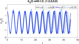
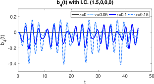
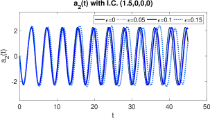
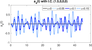
Figure 2: Solutions $b_{2}(t)$, $b_{4}(t)$, $a_{2}(t)$, $a_{4}(t)$ of (3.2)-(3.1), $t\in[0,45]$, for initial condition $(b_{1},b_{3},a_{1},a_{3})=(1.5,0,0,0)$. Black line: $\epsilon=0$. Light blue dashed line: $\epsilon=0.05$. Blue line: $\epsilon=0.1$. Gray blue dotted line: $\epsilon=0.15$.

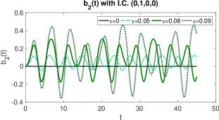
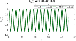
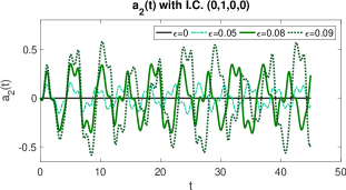
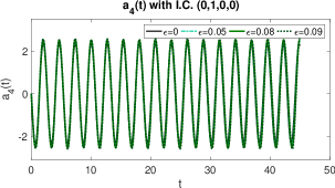
Figure 3: Solutions $b_{2}(t)$, $b_{4}(t)$, $a_{2}(t)$, $a_{4}(t)$ of (3.2)-(3.1), $t\in[0,45]$, for initial condition $(b_{1},b_{3},a_{1},a_{3})=(0,1,0,0)$. Black line: $\epsilon=0$. Light green dashed line: $\epsilon=0.05$. Green line: $\epsilon=0.08$. Dark green dotted line: $\epsilon=0.09$.

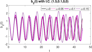
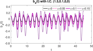
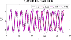
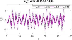
Figure 4: Solutions $b_{2}(t)$, $b_{4}(t)$, $a_{2}(t)$, $a_{4}(t)$ of (3.2)-(3.1), $t\in[0,45]$, for initial condition $(b_{1},b_{3},a_{1},a_{3})=(1.5,0.1,0,0)$. Black line: $\epsilon=0$. Pink dashed line: $\epsilon=0.05$. Violet line: $\epsilon=0.1$. Deep purple dotted line: $\epsilon=0.15$.

The numerically computed mode amplitudes $b_{2}(t)$, $b_{4}(t)$, $a_{2}(t)$, $a_{4}(t)$ are used to obtain the free surface using the spectral truncation ${\cal G}^{\epsilon}_{E,T}(s,t)$ of the approximate expression (2.11), namely

$${\cal G}^{{\epsilon}}_{E,T}(s,t)=[s+{\epsilon}\sum_{n\in\{2,4\}}b_{n}(t)\partial_{x}\Phi_{n}([s,\pi]),\pi+{\epsilon}\sum_{n\in\{2,4\}}b_{n}(t)\partial_{y}\Phi_{n}([s,\pi)],$$ (3.12)

$s\in[-\pi,\pi]$. Note that the parameter $\epsilon$ appearing in expressions for the surface, e.g. (2.11), and the spectral evolution equations (2.42), (2.43) and their truncations is the same. We may however compare the spatial shape of solutions of different dynamical equations by choosing different values for $\epsilon$ in the free surface and in the dynamical equations.

Figures 5, 6 show snapshots of the free surface for the near-monochormatic waves where the mode $n=4$ dominates, see Figure 3 with $\epsilon=0.09$. The dashed lines show the surface for a linearized model, i.e. $\epsilon=0.1$ in (3.12), and $\epsilon=0$ in the mode evolution equations (2.42)-(2.43). Figure 5 shows clearly how the boundary of the free surface follows the wall. The vertical scale used makes the wall appear almost vertical. In Figure 6 we zoom out one these snapshots using a vertical scale that makes the inclination of the wall more obvious.

The expression for the free surface (3.12) at different times allows us also to examine the spatiotemporal patterns implied by the evolution of the mode amplitudes and the shape of the normal modes. Spatiotemporal patterns for the two near-monochromatic waves with dominant mode $4$ are shown in Figure 7. Figure 7 (a) shows the smaller amplitude motions. The spatial pattern corresponds to harmonic oscillation of a single mode. In Figure 7 (b) we show the higher amplitude motions that correspond to the mode evolution of Figure 3. We see higher amplitude motions and a more complicated spatial pattern due to the presence of the second mode.

These qualitative observations of the spatial patterns can be made more precise by examining the surface elevation at a given point of the domain as a function of time and the initial amplitude. We consider the second component of ${\cal G}^{\epsilon}_{E,T}(s,t)$ of (3.12), i.e. the height of the surface, at different points $s\in[0,\pi]$. The case of $s=\pi$ is of special interest as it gives us the run-up of the waves at the beach. In Figures 8 (a), (b), (c) we show the run-up for the different initial amplitudes considered in the experiments of Figures 2 (mode $n=2$ near-monochromatic wave), 3 (mode $n=4$ near-monochromatic wave) 4 (bichromatic wave) respectively. In the case of the near-monochromatic waves, higher amplitudes lead to higher temporal variability of the amplitude, and also to lower maxima and minima. In the case of bichromatic waves we see higher temporal variability for smaller amplitudes. At $s=0$ we see a similar behavior, although local maxima and minima of the height are closer for the amplitudes examined.

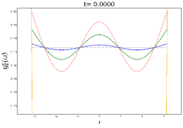
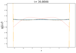
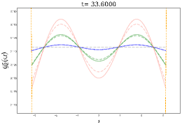
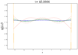
Figure 5: Surface profile of solutions at different times $t$. Solid lines: blue, $\epsilon=0.09$, initial conditions $(0,0.1,0,0)$; green, $\epsilon=0.09$, initial conditions $(0,0.5,0,0)$; pink, $\epsilon=0.09$, initial conditions $(0,1,0,0)$ (see Fig. 3). Dashed lines represent linear evolution for each initial condition.

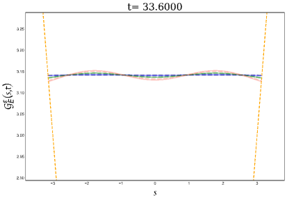
Figure 6: Zoom-out of Figure 14 at $t=33.6$.

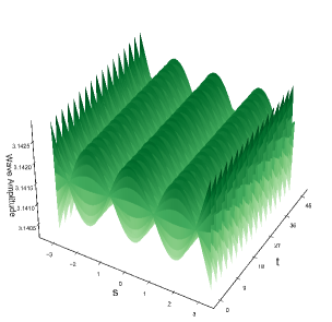
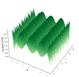
Figure 7: Spatiotemporal patterns of solutions: Left: initial condition $(b_{2},b_{4},a_{2},a_{4})=(0,0.1,0,0)$, $\epsilon=0.09$. Right: initial condition $(b_{2},b_{4},a_{2},a_{4})=(0,1,0,0)$, $\epsilon=0.09$ (see Fig. 3, dark green dotted line).

Wave run-up

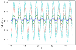
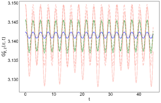
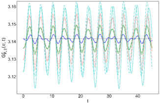
a b c

Figure 8: Run-up, i.e. second component of ${\cal G}^{\epsilon}_{E}(s,t)$ at $s=\pi$. Solid lines (common value of $\epsilon$; color, initial condition). Dashed lines correspond to linear evolution for same initial conditions. (a) $\epsilon=0.1$; blue: $(0.1,0,0,0)$, green: $(0.5,0,0,0)$, pink: $(1.0,0,0)$, light blue: $(1.5,0,0,0)$, see Fig. 2. (b) $\epsilon=0.09$; blue: $(0,0.1,0,0)$, green: $(0,0.5,0,0)$, pink: $(0,1,0,0)$, see Fig. 3. (c) $\epsilon=0.1$; blue: $(0.1,0.1,0,0)$, green: $(0.5,0.1,0,0)$, pink: $(1,0.1,0,0)$, light blue: $(1.5,0.1,0,0)$, see Fig. 4.

4 Discussion

We have derived a quadratic model for weakly nonlinear waves in a triangular channel with inclined walls of $45^{o}$ and presented calculations of phenomena such as the influence of weak nonlinearity in the wave run-up. The derivation may be valid in more general domains, assuming that a similar construction of harmonic functions related to the linear normal modes of the problem is possible in more general domains.

Justifying the steps leading to the approximate model presented for the $45^{0}$ triangular domain and possible generalizations will require additional analysis, and we have pointed out some of the problems. The representation of the free surface we proposed appears to be new, but its generality remains to be seen. Its use is justified heuristically by the fact that it leads to the linear theory (it uses an infinite set of parameters). At the same time it leads to a clear definition of the position of the free surface. In the $45^{o}$ domain the use of functions that are harmonic on the whole plane bypasses some of the regularity issues for Dirichlet-Neumann operators in domains with corners [MW16], and allows the definition of the free surface to go through. The existence of these functions is also behind a class of methods for the numerical evaluation of the Dirichlet-Neumann operator [CS93, WV15], and this is a question that could be examined further in the $45^{o}$ triangular domain. While the possibility of treating general domains is a significant motivation for this study, the question of nonlinear interactions in the geometries with known normal modes is also of interest as it also extends to three-dimensional domains.

The quadratic model and its spectral truncations pose several interesting dynamical questions. Local and global well-posedness for the quadratic model is not clear at present. Further numerical studies of spectral truncations should describe a wider range of bounded motions. The existence of nontrivial fixed points is a possible mechanism for unbounded growth in small spectral truncations. Such solutions seem tractable and can be also studied further. Extensions to cubic models may be possible. Clearly spectral models involve long intermediate calculations of mode interaction coefficients, and this is a drawback of our approach. The exact expressions for the interaction coefficients presented suggest some heuristic simplifications for short waves.

The model we presented does not have an apparent Hamiltonian structure. Work on a model with Hamiltonian structure is currently in progress. The Hamiltonian formalism involves approximation and symmetrization of a Dirichlet-Neumann operator for a perturbation of the flat surface domain. This operator was not discussed explicitly here, although we saw some operations seen in the computation of an approximate Dirichlet-Neumann operator, see Remark 2.3. The lowest order nonlinear Hamiltonian model leads to an equation that is similar in structure to the one presented here but with more complicated coefficients. Thus while the Hamiltonian structure is a desirable feature, the present model appears to be simpler. The lack of Hamiltonian structure is a drawback but also leads to interesting dynamical questions. Also, from the point of view of applications, the general structure of the evolution equations is of importance as some details could be obtained using observations.

Acknowledgments.

The authors acknowledge partial support from grant PAPIIT IN100522. R. M Vargas-Magaña also acknowledges partial support from CONACyT-Postdoctoral fellowship call EPE2019(2) and the collective “Cientificæs Mexicanæs en el Extranjero.” We also wish to thank Sebastien Fromenteau for valuable guidance with Python’s visualization tools, and Gerardo Ruiz Chavarría, Carlos García Azpeitia, and Noel F. Smyth for helpful discussions.

5 Appendix

We briefly discuss the dispersion relation and present some details of the computation of the mode interaction coefficients.

The dispersion relation can be analyzed using equations (2.28), (2.29) and the theory of Newton’s method. Details may be presented elsewhere, we here limit ourselves to showing the monotonicity of $\omega_{n}$.

Proof of Proposition 2.2: We first show monotonicity of $\omega_{n}$, $n\geq 2$. Let $n$ even then by (2.30) $\omega_{n+1}^{2}>\omega_{n}^{2}$ is equivalent to $\alpha_{n+1}\coth\alpha_{n+1}B>\alpha_{n}\tanh\alpha_{n}B$. This holds by $\alpha_{n+1}/{\alpha_{n}}>1$, see (2.28), (2.29), and $\tanh\alpha_{m}B<1$, for all $m\geq 1$.

We also need to show $\omega_{n+1}^{2}>\omega_{n}^{2}$ for $n\geq 3$ and odd, equivalently

$$\frac{\alpha_{2k+2}}{\alpha_{2k+1}}>\coth\alpha_{2k+2}B\coth\alpha_{2k+1}B.$$ (5.1)

By (2.22), (2.28) we have

$$B\alpha_{2k+2}>k\pi+\frac{3\pi}{4},$$ (5.2)

$\forall k\geq 0$, by comparing solutions of equations (2.22) and $-\tanh\alpha B=1$, and using $\tanh\alpha B<1$ and increasing in $\alpha$, and $-\tan\alpha B$ decreasing in $\alpha$. Similarly, by (2.25), (2.29) we have

$$B\alpha_{2k+1}<k\pi+\frac{\pi}{4},$$ (5.3)

$\forall k\geq 1$, by comparing solutions of (2.25) and $\tanh\alpha B=1$, and using $\tanh\alpha B<1$ and increasing, and $\tan\alpha B$ increasing. By (5.2), (5.3) we then have

$$\frac{\alpha_{2k+2}}{\alpha_{2k+1}}>\frac{4k+3}{4k+1}=1+\frac{1}{2k+\frac{1}{2}},\quad\forall k\geq 1.$$ (5.4)

On the other hand

$$\coth\alpha_{2k+2}B\coth\alpha_{2k+1}B=\left(1+\frac{2e^{-2B\alpha_{2k+1}}}{1-e^{-2B\alpha_{2k+2}}}\right)\left(1+\frac{2e^{-2B\alpha_{2k+1}}}{1-e^{-2B\alpha_{2k+1}}}\right).$$ (5.5)

By (2.28), (2.29) we have

$$e^{-2B\alpha_{2k+1}}<e^{-2k\pi},\quad e^{-2B\alpha_{2k+2}}<e^{-(2k+1)\pi},\quad\forall k\geq 1.$$ (5.6)

We simplify further by using $e^{-k}<(2k)^{-1}$, $\forall k\geq 1$, and $3<\pi$, then (5.5), (5.6) lead to

$$\coth\alpha_{2k+2}B\coth\alpha_{2k+1}B<1+\frac{3}{8k^{6}},\quad\forall k\geq 1.$$ (5.7)

Comparing (5.4), (5.7) we obtain (5.1).

It remains to show $\omega_{2}>\omega_{1}$, equivalently $B\alpha_{2}\tanh B\alpha_{2}>1$, or

$$B\alpha_{2}>\frac{1}{1-T_{2}},\quad T_{2}=\frac{2e^{-2B\alpha_{2}}}{1+2^{-2B\alpha_{2}}}.$$ (5.8)

By (5.2) we have $B\alpha_{2}>3\pi/4$, therefore $T_{2}<2e^{-3\pi/2}<2^{-3}$. Then $(1-T_{2})^{-1}<8/7$, while $B\alpha_{2}>9/4$. $\square$

Proof of Proposition 2.5: The integral $I$ left hand side of (2.52) is

$$I=\frac{1}{2}\int_{-h}^{h}[(B+\epsilon\partial_{y}V(s,B))(1+\epsilon\partial_{s}\partial_{x}V(s,B))-(s+\epsilon\partial_{x}V(s,B))(\epsilon\partial_{s}\partial_{y}V(s,B))]\;ds.$$

We split into powers of $\epsilon$

$$I=I_{0}+\epsilon I_{1}+\epsilon^{2}I_{2},$$ (5.9)

then

$$I_{0}=\frac{1}{2}\int_{-h}^{h}B\;ds=B^{2}.$$

The second term is

$$I_{1} = \frac{1}{2}\int_{-h}^{h}[-s\partial_{s}\partial_{y}V(s,B)+B\partial_{s}\partial_{x}V(s,B)+\partial_{y}V(s,B)]\;ds$$ (5.10)

$$= \int_{-h}^{h}\partial_{y}V(s,B)\;ds+\left[-s\partial_{y}V(s,B)\right]^{s=h}_{s=-h}+B\left[\partial_{x}V(s,B)\right]^{s=h}_{s=-h}.$$ (5.11)

Using the boundary condition for $V$ at $\partial{\cal W}$ we have $[1,-1]\cdot\nabla V(h,B)=0$, and $[1,1]\cdot\nabla V(-h,B)=0$ so that the boundary terms vanish. Then

$$I_{1}=\int_{-h}^{h}\partial_{y}V(s,B)\;ds=0,$$ (5.12)

by Green’s identity in the triangle defined by $[X,Y]$ and $\partial{\cal W}$, and $\Delta V=0$ in $\cal W$, ${\hat{n}}\cdot\nabla V=0$ at $\partial{\cal W}$.

The third integral in (5.9) is

$$I_{2} = \frac{1}{2}\int_{-h}^{h}[-(\partial_{x}V(s,B))\partial_{s}\partial_{y}V(s,B)+(\partial_{y}V(s,B))\partial_{s}\partial_{x}V(s,B)]\;ds$$ (5.13)

$$= -\int_{-h}^{h}\partial_{x}V(s,B)\partial_{s}\partial_{y}V(s,B)\;ds+\left[(\partial_{x}V(s,B))(\partial_{y}V(s,B))\right]^{s=h}_{s=-h}$$ (5.14)

and is not guaranteed to vanish. $\square$

References

- [AH08] M.J. Ablowitz, T.S. Haut, Spectral formulation of the two fluid Euler equations with a free interface and long wave reductions, Analysis and Applications 6, 323-348 (2008)
- [AMP13] P. Aceves-Sánchez, A.A. Minzoni, P. Panayotaros, Numerical study of a nonlocal model for water-waves with variable depth, Wave Motion 50, 80-93 (2013)
- [AN18] D. Andrade, A. Nachbin, A three-dimensional Dirichlet-to-Neumann operator for water waves over topography, J. Fluid Mech. 845, 321-345 (2018)
- [AP17] A.G. Athanassoulis, C.E. Papoutsellis, Exact semi-separation of variables in wave guides with nonplanar boundaries, Proc. R. Soc. London A 473, 20170017 (2017)
- [BB08] M. Brocchini, T. E. Baldoc, Recent advances in modeling swash zone dynamics: influence of surf-swash interaction on nearshore hydrodynamics and morphodynamics, Rev. Geophys. 46, RG3003 (2008)
- [C18] J.D. Carter, Bidirectional Whitham equations as models of waves in shallow water, Wave Motion 82, 51-62 (2018)
- [CC60] C.W. Clenshaw, A.R. Curtis, A method for numerical integration on an automatic computer, Numerische Mathematik 2,Springer,197-205 (1960).
- [C17] W. Craig, On the Hamiltonian for water waves, RIMS Kôkyûroku 2038 (2017)
- [CS93] W. Craig, C. Sulem, Numerical simulation of gravity waves, J. Comp. Phys. 108, 73-83 (1993)
- [CGNS05] W. Craig, P. Guyenne, D.P. Nicholls, C. Sulem, Hamiltonian long-wave expansions for water waves over a rough bottom, Proc. Royal Soc. London A: Math. Phys. Eng. Sci. 46, 839-873 (2005)
- [E65] D. Elliott, Truncation errors in two Chebyshev series approximations, Math. Comp. 19, 234–248 (1965)
- [EL93] D.V. Evans, C.M. Linton, Sloshing frequencies, Quart. J. Mech. Appl. Math. 46, 71–87(1993)
- [E93] G. Evans, Practical numerical integration, Wiley, Chichester (1993)
- [G87] A. G. Greenhill, Wave motion in hydrodynamics, Am. J. Math. 14, 97–112 (1887)
- [G11] P. Grisvard, Elliptic problems in nonsmooth domains, SIAM, Philadelphia (2011)
- [G94] M.D. Groves, Hamiltonian long-wave theory for water waves in a channel, Quart. J. Mech. Appl. Math. 47, 367-404 (1994)
- [G95] M.D. Groves, Theoretical aspects of gravity-capillary waves in non-rectangular channels, J. Fluid Mech. 290, 377-404 (1995)
- [HN81] C. W. Hirt, B. D. Nichols, Volume of fluid (VOF) method for the dynamics of free boundaries, J. Comp. Phys. 39, 201-225 (1981)
- [HT18] V.M. Hur, L. Tao, Wave breaking in shallow water model, SIAM J. Math. Anal. 50, 354-380 (2018)
- [H17] V.M. Hur, Wave breaking in the Whitham equation, Adv. Math. 317, 410-437 (2017)
- [L07] R.J. LeVeque, Finite difference methods for ordinary and partial differential equations, SIAM, Philadelphia (2007)
- [K79] G. Kirchhoff, Über stehende Schwigungen einer schweren Flüssigkeit, G. Kirchhoff Gesam. Abhandlungen, p. 428 (1879)
- [KH80] G. Kirchhoff, G. Hansemann, Versuche über stehende Schwigungen des Wassers, G. Kirchhoff Gesam. Abhandlungen, p. 442 (1880)
- [KMT91] D.B. Kothe, R.C. Mjolsness, M.D. Torrey, RIPPLE: A computer program for incompressible flows with free surfaces, Los Alamos Tech. Rep. LA-12007-MS (1991)
- [L32] H. Lamb, Hydrodynamics, Cambridge University Press, Cambridge (1932)
- [L13] D. Lannes, The water waves problem, AMS, Providence (2013)
- [LL89] P. Lin, P.L.F. Liu, A numerical study of breaking waves in the surf zone, J. Fluid Mech. 359, 239-264 (1989)
- [M93] H.M. Macdonald, Waves in canals, Proc. Lond. Math. Soc. 1 (1), 101–113 (1893)
- [MW16] M. Ming, C. Wang, Elliptic estimates for Dirichlet-Neumann operator on a corner domain, preprint, arXiv:1512.03271v3 (2016)
- [MKD15] D. Moldabayev, H. Kalisch, D. Dutykh, The Whitham Equation as a model for surface water waves, Physica D, 309, 99-107 (2015)
- [HA68] H. O’Hara, F.J. Smith, Error estimation in the Clenshaw–Curtis quadrature formula, Computer J. 11, 213–219 (1968)
- [P80] B.A. Packham, Small-amplitude waves in a straight channel of uniform triangular cross-section, Quart. J. Mech. Appl. Math. 33(2), 179–187 (1980)
- [P91] L. Perko, Differential equations and dynamical systems, Springer, New York (1991)
- [R68] W.C. Rheinboldt, A unified convergence theory for iterative processes, SIAM J. Num. Anal. 5, 42-63 (1968)
- [TFPP13] A. Torres-Freyermuth, J.A. Puleo, D. Pokrajac, Modeling swash-zone hydrodynamics and shear stresses on planar slopes using Reynolds-Averaged Navier–Stokes equations, J. Geophys. Res.: Oceans 118, 1019-1033 (2013)
- [T00] L.N. Trefethen, Spectral methods in MATLAB, SIAM, Philadephia (2000).
- [VMS21] R.M. Vargas-Magaña, T. Marchant, N.F. Smyth, Numerical and analytical study of undular bores governed by the full water-wave equations and bi-directional Whitham-Boussinesq equations, Phys. Fluids 33, 067105 (2021)
- [VP16] R.M. Vargas-Magaña, P. Panayotaros, A Whitham-Boussinesq long-wave model for variable topography, Wave Motion 65, 156-174 (2016)
- [VMMP19] R.M. Vargas-Magaña, A. Minzoni, P. Panayotaros, Linear Whitham-Boussinesq modes in channels of constant cross-section, Water Waves, 1, 1-28 (2019)
- [WV15] J. Wilkening, V. Vasan, Comparison of five methods to compute the Dirichlet-Neumann operator for the water wave problem, Contemp. Math. 635, 175-210 (2015)
- [Z86] E. Zeidler, Nonlinear functional analysis and its applications I, Springer, New York (1986)