Critical Balance and Scaling of Strongly Stratified Turbulence at Low Prandtl Number

Abstract

We extend the scaling relations of strongly (stably) stratified turbulence from the geophysical regime of unity Prandtl number to the astrophysical regime of extremely small Prandtl number applicable to stably stratified regions of stars and gas giants. A transition to a new turbulent regime is found to occur when the Prandtl number drops below the inverse of the buoyancy Reynolds number, i.e. $PrRb<1$, which signals a shift of the dominant balance in the buoyancy equation. Application of critical balance arguments then derives new predictions for the anisotropic energy spectrum and dominant balance of the Boussinesq equations in the $PrRb\ll 1$ regime. We find that all the standard scaling relations from the unity $Pr$ limit of strongly stratified turbulence simply carry over if the Froude number, $Fr$, is replaced by a modified Froude number, $Fr_{M}\equiv Fr/(PrRb)^{1/4}$. The geophysical and astrophysical regimes are thus smoothly connected across the $PrRb=1$ transition. Applications to vertical transport in stellar radiative zones and modification to the instability criterion for the small-scale dynamo are discussed.

1 Introduction

Turbulence in the strongly stratified regions of planetary oceans, atmospheres and the interiors of stars and gas giants provides an important source of vertical transport of chemicals and momentum, thereby playing a critical role in their long-term evolution (zahn1974rotational; zahn1992circulation; fernando1991turbulent; pinsonneault1997mixing; maeder2000evolution; ivey2008density; ferrari2009ocean; aerts2019angular; garaudJtCS2021). However, current understanding of the extremely low thermal Prandtl number regime of astrophysical turbulence remains disjoint from the order unity Prandtl number regime of geophysical turbulence. This is despite identical asymptotic limits for the Reynolds $Re\gg 1$, Froude $Fr\ll 1$, and buoyancy Reynolds $Rb=ReFr^{2}\gg 1$ numbers. The Prandtl number $Pr=\nu/\kappa$ measures the ratio of the microscopic viscosity $\nu$ to the thermal diffusivity $\kappa$ and is extremely small in stellar plasma in particular. Photons rapidly diffuse heat compared to the much slower momentum diffusion by ion-ion collisions, leading to $\kappa\gg\nu$. For reference, stellar radiative zones have Prandtl numbers that can range from $Pr=O(10^{-9})$ to at most $Pr=O(10^{-5})$, in contrast to Earth’s fluids that range from $Pr\simeq 0.7$ in the atmosphere to $Pr\simeq 10$ in the ocean (garaudJtCS2021). A Prandtl number as high as $Pr\simeq 700$ can be reached in parts of the ocean dominated by salt-stratification (thorpe2005turbulent; gregg2018mixing; gregg2021ocean) (where the salt diffusivity replaces thermal diffusivity). Compared to the $Pr=1$ case, a small $Pr$ can have significant effects on large-scale hydrodynamic instabilities and the resulting turbulence (garaudJtCS2021) while a large $Pr$ influences scales comparable to and smaller than the viscous scale and can have significant effects on the buoyancy flux, mixing efficiency, and properties of shear-induced turbulence (salehipour2015turbulent; legaspi2020prandtl; okino2020direct).

Many important features of the unity Prandtl number regime are becoming better understood from a combination of numerical experiments (waite2004stratified; brethouwer2007; riley2010recent; maffioli2016dynamics; lucas2017layer; de2019effects), observational data (lindborg2007stratified; riley2008stratified; falder2016seismic; lefauve2022experimental), and theoretical developments (billant2001self; lindborg2006; chini2022exploiting). Strongly stratified turbulence with $Pr=O(1)$ forced at some horizontal length scale leads to emergent vertical scales set by the stratification and exhibits two distinct inertial ranges that transfer energy from the large forcing scales to the small viscous and thermal scales where it is dissipated. The transition length scale between the two ranges is known as the Ozmidov scale (ozmidov1992variability). The turbulence is highly anisotropic from the outer forcing scale down to the Ozmidov scale with the down-scale energy transfer likely containing contributions from both a local energy cascade and non-local energy transfer mechanisms (e.g. shear instabilities, wave-wave interactions) (Waite2011; augier2015stratified; maffioli2016dynamics; khani2018mixing). Below the Ozmidov scale, the turbulence is isotropic down to the diffusive scales. Properties of the energy cascade, relevant dimensionless parameters, and scaling relations for the emergent vertical scales are now fairly well understood, although many further questions remain such as on the efficiency of mixing (gregg2018mixing; monismith2018mixing; legg2021mixing) and the origin of self-organized criticality (smyth2013marginal; salehipour2018self; smyth2019self; chini2022exploiting; lefauve2022experimental).

The main aim of this study is to extend the theoretical arguments used in the $Pr=O(1)$ regime to make analogous predictions for the emergent vertical scales and energy cascades in the asymptotically low $Pr$ regime. If only the thermal diffusivity is increased while keeping all other parameters constant (thereby decreasing $Pr$), one should expect a smooth transition to occur between two asymptotic regimes when thermal diffusion shifts from being important only on the smallest, viscous scales to playing an important role on the mesoscales i.e. on scales comparable to or larger than the Ozmidov scale.

To understand this transition, we use the critical balance framework proposed by Nazarenko2011 for anisotropic wave systems. Critical balance argues that linear wave $\omega^{-1}$ and non-linear interaction $\tau_{\mathrm{NL}}$ time scales are comparable $\omega^{-1}\sim\tau_{\mathrm{NL}}$ on a scale-by-scale basis throughout a local energy cascade, giving a prediction for the anisotropy of the turbulence as a function of scale. Originally applied in mean field MHD turbulence (goldreich1995toward) (also see schekochihin2022mhd and references within), critical balance successfully predicts power laws of the anisotropic energy spectra and associated transition scales in rotating turbulence and unity Prandtl number strongly stratified turbulence (Nazarenko2011).

We propose that critical balance should naturally extend to low thermal Prandtl number strongly stratified turbulence with a modification in its physical interpretation. As $Pr$ is decreased (by increasing $\kappa$ while keeping $\nu$ small and fixed), the full internal gravity wave (IGW) dispersion $\omega$ smoothly transitions from the asymptotic dispersion for adiabatic, inviscid, propagating IGWs when $Pr=O(1)$ ($\omega\sim\omega_{\mathrm{N}}$) to an asymptotic dispersion for overdamped, inviscid, IGWs modified by the interaction of buoyancy and fast thermal diffusion when $Pr\ll 1$ ($\omega\sim\omega_{\mathrm{lPe}}$, where “lPe” refers to the “low turbulent Peclet” limit as discussed in more detail in Sections 2 and 4). As a result, scaling laws for the emergent vertical scales and two cascades predicted by critical balance will likewise smoothly change as $Pr$ is decreased. We note that because critical balance assumes a local energy cascade, the relative role of non-local energy transfer mechanisms in the low $Pr$ limit remains to be understood.

1.1 Paper Layout

The Boussinesq equations used to model stably stratified turbulence are defined in Section 2 followed by an argument for when a transition of turbulence regimes should occur. Critical balance arguments in the unity $Pr$ regime are reviewed in Section 3 to then compare with the new critical balance arguments in the low $Pr$ regime given in Section 4. Astrophysical applications of the new scaling laws are discussed in Section LABEL:sec:Applications.

2 The Boussinesq Approximation and the $PrRb=1$ Transition

2.1 The Boussinesq Approximation

Stably stratified regions of stars and gas giants below their surfaces typically sustain turbulent motions with vertical length scales that are small compared to the local scale height and velocity fluctuations are that small compared to the local sound speed. In this limit, the Spiegel-Veronis-Boussinesq equations are a rigorous approximation for the fluctuations of the velocity field and thermodynamic variables of a compressible fluid on top of a stably stratified background (spiegel1960boussinesq). The approximation effectively filters out the high frequencies of sound waves compared to the lower frequencies of internal gravity waves and fluid motions of interest. The governing equations for the velocity field $\textbf{u}^{\prime}$ and the buoyancy variable $\theta^{\prime}=\alpha gT^{\prime}=-\rho^{\prime}g/\rho_{m}$ are: ∂_t u’+u’⋅∇u’&=-1ρm∇p’+θ’^z+ν∇^2 u’,
∂_t θ’+u’⋅∇θ’=-N^2u_z’+κ∇^2θ’,
∇⋅u’=0, where $\alpha$ is the coefficient of thermal expansion, $g$ is the local gravitational constant, $T^{\prime}$ is the temperature perturbation, $\rho^{\prime}$ is the density perturbation, $\rho_{m}$ is the mean density of the region, $p^{\prime}$ is the pressure perturbation, and $N$ is the local Brunt-Väisälä frequency. Primed variables here denote dimensional quantities and unprimed variables will later denote dimensionless quantities. Note that the Brunt-Väisälä frequency captures all the relevant local thermodynamics of the medium in the Boussinesq approximation of any fluid (bois1991asymptotic). As a result, the above equations are formally equivalent to those used in geophysical fluid studies of the Earth’s oceans, but with a different definition of $N$. For example, in the case of an ideal gas $N^{2}=\alpha g(\partial_{z}\bar{T}-\partial_{z}T_{\rm ad})$ while in the case of a liquid $N^{2}=-g\partial_{z}\bar{\rho}/\rho_{m}$, where $\partial_{z}\bar{\rho}$, $\partial_{z}\bar{T}$, and $\partial_{z}T_{\rm ad}$ are the background density, background temperature, and adiabatic temperature gradients, respectively.

2.2 Geophysical Regime

A stably stratified fluid forced on a horizontal length $L$ and velocity scale $U$ leads to turbulence with an emergent outer vertical length $l_{z}$ and velocity scale $u_{z}$ set by the physical parameters of the fluid {$N$, $\nu$, $\kappa$}. From dimensional analysis, only three dimensionless parameters characterize the fluid: the Reynolds number $Re=UL/\nu$, the Froude number $Fr=U/NL$, and the Prandtl number $Pr=\nu/\kappa$. Understanding the scaling of the emergent outer vertical scales as well as the structure of the subsequent (anisotropic) energy cascade is an important theoretical and experimental goal.

In the geophysical fluid regime where $Pr=O(1)$, evidence from theoretical arguments, simulations, and experimental data strongly suggests that the outer vertical length and vertical scales are directly set by the Froude number when the viscosity is sufficiently small: $l_{z}\sim FrL$ and $u_{z}\sim FrU$, where $l_{z}$ is often called the buoyancy length scale. Strong stratification ($Fr\ll 1$) thus leads to highly anisotropic structures of the large scale eddies characterized by long horizontal scales and short vertical scales as well as significantly more energy in the horizontal compared to the vertical velocity components. The injected energy undergoes an anisotropic forward energy cascade at large length scales until the Ozmidov scale, an intermediate scale given by $l_{O}=Fr^{3/2}L$ (brethouwer2007). For scales smaller than $l_{O}$, the effects of buoyancy are negligible on the fast turn over times of the eddies and an isotropic Kolmogorov cascade operates down to the dissipation scales, which are the viscous ($l_{\nu}=Re^{-3/4}L$) and thermal ($l_{\kappa}\simeq l_{\nu}$) scales. The range of the isotropic cascade is set by the buoyancy Reynolds number $Rb=ReFr^{2}$ ($l_{O}/l_{\nu}=Rb^{3/4}$) and needs to be sufficiently large in order to support the two cascades characteristic of strongly stratified turbulence (bartello2013sensitivity).

The horizontal and vertical scales from above in the limits $Fr\ll 1$ and $Rb\gg 1$ suggest a consistent rescaling of the Boussinesq equations using the following dimensionalization (identical to billant2001self):

u_h’=U u_h, u_z’=FrUu_z, θ’=1FrU2Lθ, p’= ρ_m U^2p,
x’=Lx, y’=L y, z’=FrL z, t’=LU t, where the scaling of $\theta^{\prime}$ is determined by a balance of $\textbf{u}^{\prime}\cdot\nabla\theta^{\prime}\sim N^{2}u_{z}^{\prime}$ since thermal diffusivity is considered to be sufficiently small. Substituting the above, the Boussinesq equations become:

∂_t u_h+u⋅∇u_h&=-∇_h p+ [1Re∇_h^2+1Rb∇_z^2]u_h,
Fr^2[∂_t u_z+u⋅∇u_z]=-∇_z p+θ+Fr^2[1Re∇_h^2+1Rb∇_z^2]u_z,
∂_tθ+u⋅∇θ=-u_z+[1PrRe∇_h^2+1PrRb∇_z^2]θ,
∇⋅u=0, where $\textbf{u}_{h}$ and $\nabla_{h}$ denote the horizontal components of the velocity and gradient. Note that $Rb$ and $PrRb$ act as effective Reynolds numbers in the vertical part of the momentum and thermal diffusion terms, respectively. Examination of the dominant balance to lowest order is helpful:

∂_t u_h+u⋅∇u_h&=-∇_h p,
0=-∇_z p+θ,
∂_t θ+u⋅∇θ=-u_z,
∇⋅u=0,

Advection in the horizontal momentum equation (Eq 2.2a) is balanced by horizontal pressure gradients, while the dominant balance in the vertical momentum equation (Eq 2.2b) is instead between the vertical pressure gradient and buoyancy fluctuations. These balances will change if the viscosity is increased and the vertical gradients of the momentum diffusion term become important. Further, the buoyancy equation (Eq. 2.2c) is a balance between temperature advection and displacement of the fluid against the background stratification gradient. It is this latter balance that will change if thermal diffusion is increased and the vertical gradients of the thermal diffusion term become important, as we show in the next section.

2.3 Transitions from the Geophysical Regime

We now aim to understand when transitions occur from the regime of geophysical fluid turbulence where $Fr\ll 1$, $Rb\gg 1$, and $Pr=O(1)$. First, lets consider the better understood transition to the viscosity-affected stratified flow regime as $Re$ is decreased with fixed $Fr$ and $Pr=O(1)$ (godoy2004vertical). The case of decreasing $Pr$ turns out to behave in an analogous manner. From the perspective of the turbulent cascades, as viscosity is increased, the viscous scale will grow until it is comparable to the Ozmidov scale $l_{\nu}\sim l_{O}$, at which point $Rb\sim 1$ and the isotropic cascade at small scales disappears (brethouwer2007). This appears as a shift of the dominant balance in the horizontal momentum equation (Eq 2.2a) between advection and the vertical gradient of the momentum diffusivity:

$$\frac{\textbf{u}^{\prime}\cdot\nabla\textbf{u}_{h}^{\prime}}{\nu\nabla_{z}^{2}\textbf{u}_{h}^{\prime}}\sim\frac{u_{z}l_{z}}{\nu}\sim ReFr^{2}=Rb$$ (1)

where vertical and horizontal advection are comparable due to the incompressibility constraint (i.e. $u_{z}/l_{z}\sim U/L$) and $l_{z}/L\sim u_{z}/U\sim Fr$ is used to estimate the vertical scales near $Rb\sim 1$. Heuristically, $Rb$ is the ratio of the eddy turnover rate to the viscous diffusion rate at the outer vertical scales, i.e. $Rb\sim(u_{z}/l_{z})/(\nu/l_{z}^{2})$. For $Rb<1$, a change of dominant balance ($\textbf{u}^{\prime}\cdot\nabla\textbf{u}_{h}^{\prime}\sim\nu\nabla_{z}^{2}\textbf{u}_{h}^{\prime}$) leads to an alternative scaling $l_{z}/L=Fr/Rb^{1/2}$ (usually written as $l_{z}/L\sim Re^{-1/2}$) where viscosity dominates the coupling of adjacent vertical layers. The same shift occurs in the buoyancy equation ($N^{2}u_{z}^{\prime}\sim\kappa\nabla_{z}^{2}\theta^{\prime}$) and the new vertical velocity scale becomes $u_{z}/U\sim FrRb^{1/2}$ (derived with $\theta^{\prime}\sim\nabla_{z}p^{\prime}/\rho_{m}$ from the unchanged dominant balance in the vertical momentum equation). This regime is often reached by simulations because computational constraints limit how small the viscosity can be set. Note that the vertical scales smoothly transition from $l_{z}/L\sim u_{z}/L\sim Fr$ at $Rb=1$ as $Rb$ is decreased.

Returning to the physically interesting limit $Fr\ll 1$ and $Rb\gg 1$ of strongly stratified turbulence, we now consider the effect of decreasing $Pr$ at fixed $Re$ and $Fr$, equivalent to increasing the thermal diffusivity while keeping the viscosity fixed. From the perspective of the turbulent cascades, as thermal diffusivity is increased, the thermal scale $l_{\kappa}\sim(PrRe)^{-3/4}L$ will grow until it is comparable to the Ozmidov scale $l_{\kappa}\sim l_{O}$, at which point $PrRb\sim 1$ and thermal diffusion becomes important on mesoscales that are influenced by buoyancy forces (lignieres2019turbulence). This appears as a shift of the dominant balance only in the buoyancy equation (Eq. 2.2c) between advection and the vertical gradient of thermal diffusion:

$$\frac{\textbf{u}^{\prime}\cdot\nabla\theta^{\prime}}{\kappa\nabla_{z}^{2}\theta^{\prime}}\sim\frac{u_{z}l_{z}}{\kappa}\equiv Pe_{t},$$ (2)

where $Pe_{t}$ is the turbulent Peclet number, which can be interpreted heuristically in a similar way to $Rb$ as the ratio of the eddy turnover rate to the thermal diffusion rate at the outer vertical scales, i.e. $Pe_{t}=(u_{z}/l_{z})/(\kappa/l_{z}^{2})$. If we use the scalings $l_{z}/L\sim u_{z}/U\sim Fr$ from the $Pr=O(1)$ regime to estimate $Pe_{t}$ in the geophysical regime, we see that $Pe_{t}\sim PrRb$ and so the transition from $Pe_{t}>1$ to $Pe_{t}<1$ occurs around $PrRb\sim 1$, exactly like the $l_{\kappa}\sim l_{O}$ transition discussed above. Thus, thermal diffusion will cause a transition in turbulent regimes if $PrRb<1$. The scalings for $u_{z}$ and $l_{z}$ from the $PrRb>1$ regime will then change (the scaling for $Pe_{t}$ will correspondingly change as well).

The emergent turbulent Peclet number is a more important parameter than the standard Peclet number $Pe=PrRe$ (zahn1992circulation; lignieres2019turbulence; cope2020dynamics), which measures the ratio of advection to the horizontal gradient of thermal diffusion: $(\textbf{u}^{\prime}\cdot\nabla\theta^{\prime})/(\kappa\nabla_{h}^{2}\theta^{\prime})\sim UL/\kappa$. This is because $Pe_{t}\ll Pe$—thermal diffusion will always be more important in the vertical than horizontal direction. In astrophysical systems, the extremely large Reynolds numbers often keep $Pe\gg 1$ despite small Prandtl numbers. As a canonical example, turbulence from horizontal shear instabilities in the solar tachocline approximately sustain $Re=O(10^{14})$ and $Pe=O(10^{8})$ using $Pr=O(10^{-6})$ (garaud2020horizontal). Thus horizontal thermal diffusion is likely less important on outer scales in other stars as well. On the other hand, we find $PrRb=O(10^{1})$ (and hence $Pe_{t}=O(10^{1})$) by using $Fr\sim 3\cdot 10^{-4}$ and $Rb\sim O(10^{7})$. The near unity value of $Pe_{t}$ shows that vertical thermal diffusion can easily become relevant in the astrophysical case (garaudJtCS2021), in particular, in stars with much lower $Pr$ (down to $Pr=O(10^{-9})$ in some stars), stronger background stratification (higher $N$), or weaker driving (lower $U$ or larger $L$). Interestingly, these values of $Re$, $Fr$, and $Rb$ are similar to those found in Earth’s atmosphere (lilly1983stratified; waite2014direct).

An important asymptotic model known as the low Peclet approximation is often used to study the $Pe_{t}<1$ regime (lignieres1999small). It can be derived from the shift in dominant balance in the buoyancy equation. If $Pe_{t}\ll 1$, then the $-N^{2}u_{z}^{\prime}$ term balances $\kappa\nabla^{2}\theta^{\prime}$ instead of $\textbf{u}^{\prime}\cdot\nabla\theta^{\prime}$. In other words, to lowest order, buoyancy fluctuations are generated by vertical advection of the mean background profile while advection of the buoyancy fluctuations is unimportant because of rapid thermal diffusion. As a result, the buoyancy fluctuations can be solved for directly $\theta^{\prime}=\frac{N^{2}}{\kappa}\nabla^{-2}u_{z}^{\prime}$. This is substituted back into Eq 1a to get a closed momentum equation:

$$\partial_{t}\textbf{u}^{\prime}+\textbf{u}^{\prime}\cdot\nabla\textbf{u}^{\prime}=-\frac{1}{\rho_{m}}\nabla p^{\prime}+\frac{N^{2}}{\kappa}\nabla^{-2}u_{z}^{\prime}\hat{z}+\nu\nabla^{2}\textbf{u}^{\prime},\quad\nabla\cdot\textbf{u}^{\prime}=0$$ (3)

There are now only two dimensional parameters $N^{2}/\kappa$ and $\nu$, which, along side the imposed $U$ and $L$, imply that the scaling in this limit can only be functions of the dimensionless parameters $PeFr^{-2}=PrRb/Fr^{4}$ and $Re$ (lignieres2019turbulence; cope2020dynamics).

The discussion so far has argued that the geophysical regime with $Fr\ll 1$, $Rb\gg 1$, and $PrRb>1$ can transition either to a flow dominated by viscous effects when $Rb<1$ or to stratified turbulence modified by thermal diffusion when $PrRb<1$. These transitions correspond to the effective Reynolds numbers of the vertical part of the momentum and thermal diffusion terms becoming smaller than unity, respectively. Our aim is now to derive a formal scaling for the astrophysically motivated $PrRb<1$ regime with the help of the critical balance hypothesis, but first we review critical balance arguments for the geophysical $PrRb>1$ regime.

3 Critical Balance and Scaling for $PrRb>1$

We derive here the standard scaling relations for the limit of $Fr\ll 1$, $Rb\gg 1$, and $PrRb>1$ using critical balance arguments. Consider a stably stratified fluid where energy is injected with power $P$ at a low wavenumber $k_{f}=2\pi/L$ and sustains turbulence with a kinetic energy dissipation rate $\epsilon\sim P\sim U^{3}/L$, where $U$ and $L$ are the outer horizontal velocity and length scales. Viewing anisotropic structures in the turbulence as a function of horizontal scale $k_{\perp}^{-1}$, the goal is to find the characteristic vertical scale $k_{\parallel}^{-1}$ associated with each $k_{\perp}$. Here $k_{\parallel}$ and $k_{\perp}$ are wavenumbers parallel and perpendicular to the direction of gravity, respectively. Such a structure will have an associated linear timescale $\omega^{-1}$ related to the wave dispersion and a non-linear timescale $\tau_{\rm NL}$ related to the self-straining timescale. We discuss estimation of both timescales for the $PrRb>1$ case before applying critical balance arguments that connect $k_{\perp}$ and $k_{\parallel}$.

The Boussinesq system supports linear motions with a dispersion relation given by $\omega(k_{\parallel},k_{\perp})$. In the limit of arbitrarily small viscosity and thermal diffusivity, wave damping is negligible ($\nu k^{2},\kappa k^{2}\ll\omega$) and the linear motions are propagating waves closely approximated by adiabatic, inviscid IGWs with dispersion $\omega\approx\omega_{\mathrm{N}}=Nk_{\perp}/k$. Because large scale vertical motion is strongly restricted, the vertical scales are much finer than the horizontal scales with an anisotropy at large scales quantified by $k_{\perp}/k_{\parallel}\ll 1$. The linear wave frequency is then approximately:

$$\omega_{\mathrm{N}}\approx\frac{Nk_{\perp}}{k_{\parallel}}$$ (4)

On the other hand, non-linear interactions breakup eddies and transfer energy from larger to smaller scales, setting up a cascade from the forcing to the diffusive scales where the energy is dissipated. Non-linear interactions occur via the advection term $\textbf{u}\cdot\nabla\textbf{u}$. Incompressibility $\nabla\cdot\textbf{u}=0$ requires $\nabla_{\parallel}u_{\parallel}\sim\nabla_{\perp}u_{\perp}$ and allows the estimate $\textbf{u}\cdot\nabla\textbf{u}\simeq\textbf{u}_{\perp}\cdot\nabla\textbf{u}_{\perp}\simeq\textbf{u}_{\parallel}\cdot\nabla\textbf{u}_{\perp}$, where $u_{\parallel}$ and $u_{\perp}$ are the scale dependent vertical and horizontal velocities, respectively. The non-linear interaction time scale using the perpendicular non-linearity is given by:

$$\tau_{\mathrm{NL}}^{-1}\sim k_{\perp}u_{\perp}(k_{\perp})$$ (5)

The scaling of $\tau_{\rm NL}$ with $k_{\perp}$ can be found if a separate relation can connect $u_{\perp}$ and $\tau_{\rm NL}$. This comes from assuming that a local (in scale) cascade brings energy down from larger to smaller scales with a “cascade time” $\tau_{\mathrm{cas}}(k_{\perp})$ that determines the energy spectrum $E(k_{\perp})$:

$$k_{\perp}E(k_{\perp})\sim u_{\perp}^{2}(k_{\perp})\sim\epsilon\tau_{\mathrm{cas}}(k_{\perp})$$ (6)

A relation between $\tau_{\rm cas}$ and $\tau_{\rm NL}$ would provide the desired $\tau_{\rm NL}(k_{\perp})$.

In homogeneous, isotropic turbulence the only dimensional option is to set $\tau_{\mathrm{cas}}\sim\tau_{\mathrm{NL}}$, which results in the standard Kolmogorov scalings $u_{\perp}(k_{\perp})\sim(\epsilon/k_{\perp})^{1/3}$, $\tau_{\rm NL}\sim(L/U)(k_{\perp}L)^{-2/3}$, and $E(k_{\perp})\sim\epsilon^{2/3}k_{\perp}^{-5/3}$. In anisotropic turbulence, the two additional dimensionless parameters $k_{\parallel}/k_{\perp}$ and $\omega\tau_{\mathrm{NL}}$ no longer constrain the system and the energy spectrum and cascade time can be an arbitrary function of these dimensionless groups. A further physically-motivated constraint is needed.

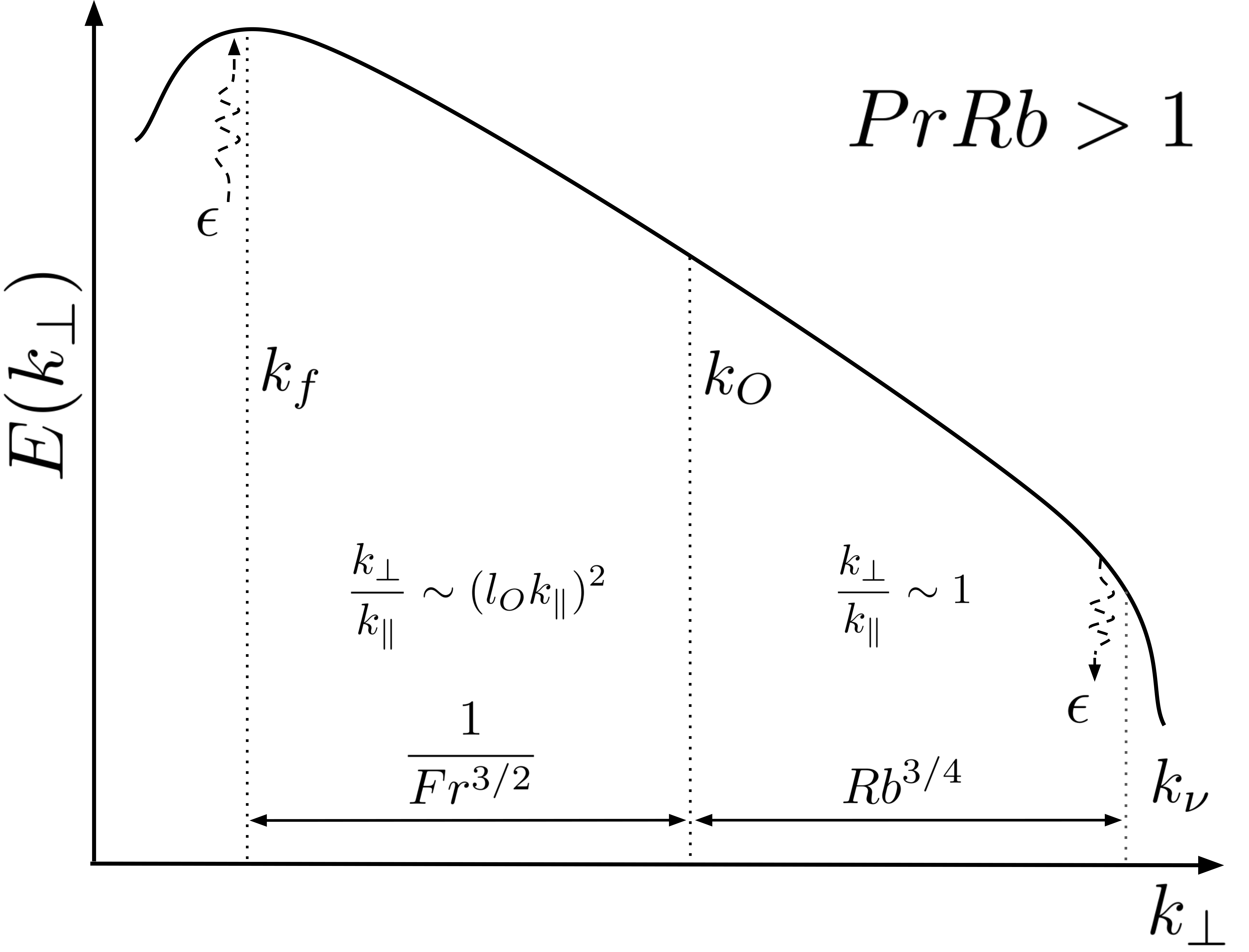
Figure 1: Energy cascade in strongly stratified turbulence for $PrRb\gg 1$ relevant to the $Pr=O(1)$ regime of Earth’s atmosphere and ocean. $E(k_{\perp})$ is the horizontal energy spectrum of the velocity field. Energy is injected at low wavenumber $k_{f}$ (large scales) with power $P\sim\epsilon$ and undergoes a forward cascade down to dissipation scales. An anisotropic cascade results across horizontal wavenumbers in the range $k_{f}\lesssim k_{\perp}\lesssim k_{O}$ with associated vertical wavenumbers in the range $2\pi/l_{z}\lesssim k_{\parallel}\lesssim k_{O}$. An isotropic cascade follows for wavenumbers larger than $k_{O}$ up to the dissipation wavenumber $k_{\nu}$. The strength of the anisotropy is quantified by $k_{\perp}/k_{\parallel}$.

Nazarenko2011 propose critical balance as a universal scaling conjecture for strong turbulence in anisotropic wave systems. Critical balance states that the linear propagation $\omega^{-1}$ and the non-linear interaction time scales $\tau_{\mathrm{NL}}$ are approximately equal $\omega\tau_{\mathrm{NL}}\sim 1$ on a scale by scale basis at all scales where the source of anisotropy is important. Physically, this in essence is a causality argument in a system where the perpendicular non-linearity dominates (e.g. rotating turbulence, MHD with a mean field): a fluctuation with some $k_{\perp}$ cannot maintain an extent longer than $k_{\parallel}^{-1}$ set by requiring the linear propagation time in the parallel direction to be comparable to the non-linear breakup time in the horizontal direction. However, the causality argument is more complicated in stably stratified turbulence (Nazarenko2011) because the non-linearity has equal strength in the parallel and perpendicular directions $\tau_{\rm NL}\sim k_{\perp}u_{\perp}\sim k_{\parallel}u_{\parallel}$, so one could equally argue a balance between linear propagation time in the perpendicular direction and non-linear breakup time in the vertical. In either case, since the group velocity sets the propagation speed of information, the linear timescale across either the parallel or perpendicular extent of a fluctuation is $(k_{\perp}v_{g,\perp})^{-1}\sim(k_{\parallel}v_{g,\parallel})^{-1}\sim\omega_{N}^{-1}$. Several physical mechanisms are known to be consistent with critical balance including zigzag (billant2000experimental; billant2000theoretical) and shear instabilities (see Section LABEL:sec:VerticalShearInst), however a complete physical picture is still an area of investigation (see further discussions in lindborg2006). Going forward, we assume the critical balance hypothesis and that IGWs effectively set the linear propagation timescale in the $PrRb>1$ limit.

Critical balance removes the ambiguity in determining the cascade time scale (i.e. $\tau_{\mathrm{cas}}\sim\tau_{\mathrm{NL}}$), which results in a Kolmogorov spectrum for the horizontal spectrum at all scales. The vertical spectrum can then be easily determined from $E(k_{\parallel})k_{\parallel}\sim E(k_{\perp})k_{\perp}$ once $k_{\perp}$ and $k_{\parallel}$ are related. Applying critical balance $\omega_{N}\tau_{\rm NL}\sim 1$ and rearranging gives the relation between $k_{\perp}$ and $k_{\parallel}$:

$$k_{\perp}\sim\left(\frac{\epsilon}{N^{3}}\right)k^{3}_{\parallel}=l_{O}^{2}k_{\parallel}^{3}$$ (7)

where $l_{O}=(\epsilon/N^{3})^{1/2}=k_{O}^{-1}$ is the Ozmidov scale. The anisotropy $k_{\perp}/k_{\parallel}\sim(l_{O}k_{\parallel})^{2}$ decreases at smaller scales until the Ozmidov scale $k^{-1}\sim l_{O}$ where the turbulence returns to isotropy $k_{\perp}\sim k_{\parallel}$ and $\tau_{\mathrm{NL}}^{-1}\sim N$. The Ozmidov scale is thus the largest horizontal scale that can overturn before restoration by buoyancy forces becomes significant. The horizontal and vertical spectrum for $k<k_{O}$ are then:

$$\frac{E(k_{\perp})}{U^{2}L}\sim(k_{\perp}L)^{-5/3},\quad\frac{E(k_{\parallel})}{U^{2}L}\sim Fr(k_{\parallel}l_{z})^{-3}$$ (8)

These energy spectra agree with the theoretical scaling predictions in the geophysical literature (dewan1997saturated; billant2001self; lindborg2006), where the parallel energy spectrum is often written in a dimensional form as $E(k_{\parallel})\sim N^{2}k_{\parallel}^{-3}$.

The turbulence no longer feels the large scale stratification gradients below the Ozmidov scale since $\omega_{\mathrm{N}}\tau_{\mathrm{NL}}\ll 1$ for $k\gg k_{O}$. Consequently, an isotropic Kolmogorov cascade results at small scales because $\tau_{\mathrm{NL}}$ becomes the only dimensionally available timescale (i.e. the slow buoyancy restoration timescale is irrelevant). The isotropic cascade extends from $k_{O}$ to the viscous wavenumber $k_{\nu}$ where $\tau_{\mathrm{NL}}^{-1}\sim\nu k^{2}\rightarrow l_{\nu}\sim(\nu/\epsilon^{1/3})^{3/4}$. As a result, the vertical spectrum has break at $k\sim k_{O}$ from $k_{\parallel}^{-3}$ to $k_{\parallel}^{-5/3}$ while the horizontal spectrum remains $k_{\perp}^{-5/3}$ throughout. The temperature thus plays an important role providing buoyancy for scales $k<k_{O}$ but is simply advected as a passive scalar for scales $k>k_{O}$ until it is dissipated at thermal diffusion scales.

For clarity, it is useful to summarize the energy cascade in terms of the dimensionless parameters $Fr$ and $Re$. Energy injected at large horizontal scales $L$ undergoes an anisotropic cascade until the Ozmidov scale, $l_{O}=Fr^{3/2}L$. Following the anisotropic cascade is an isotropic cascade down to the viscous scale, which can be written as $l_{\nu}=Re^{-3/4}L$. The size of the isotropic cascade is $l_{O}/l_{\nu}=Rb^{3/4}$. $Rb$ essentially plays the role of the effective Reynolds number for the isotropic cascade with outer length scale $l_{O}$ and velocity scale $u_{\parallel}(k_{O})=(\epsilon l_{O})^{1/3}=Fr^{1/2}U$ (i.e. $Rb=u_{\parallel}(k_{O})l_{O}/\nu$). A schematic of the energy cascade in terms of dimensionless parameters is shown in Figure 1.

Critical balance has provided a prediction for the anisotropy in the energy cascade for $Rb\gg 1$ and can therefore also predict the scaling of the outer vertical length and velocity scales of the system by considering the largest scales of the cascade. Substituting $k_{\perp}\sim 1/L$ and $k_{\parallel}\sim 1/l_{z}$ into Eq 7 predicts that $l_{z}\sim FrL$ for the outer vertical length scales. Enforcing incompressibility $u_{\parallel}\sim(k_{\perp}/k_{\parallel})u_{\perp}$ subsequently predicts that $u_{z}=u_{\parallel}(2\pi/L)\sim FrU$ for the outer vertical velocity scale. These are exactly the scaling relations discussed in Section 2.2—critical balance successfully reproduces the known scaling relations in the $PrRb>1$ regime.

4 Critical Balance and Scaling for $PrRb<1$

We turn to deriving scaling relations in the $PrRb<1$ regime by extending the critical balance arguments presented in the previous section. The idea is to replace the adiabatic, inviscid IGW frequency $\omega_{\mathrm{N}}$ with the corresponding frequency in the low (turbulent) Peclet limit $\omega_{\mathrm{lPe}}$ for the estimate of the linear timescale. A linear analysis of the Boussinesq equations with $\nu=0$ and $\kappa\neq 0$ modeling the $Pr\ll 1$ limit gives a dispersion relation:

$$\omega^{2}-i\omega\gamma_{\kappa}-\omega_{\mathrm{N}}^{2}=0,\quad\gamma_{\kappa}=\kappa k^{2},\;\omega^{2}_{N}=N^{2}\frac{k^{2}_{\perp}}{k^{2}}$$ (9)

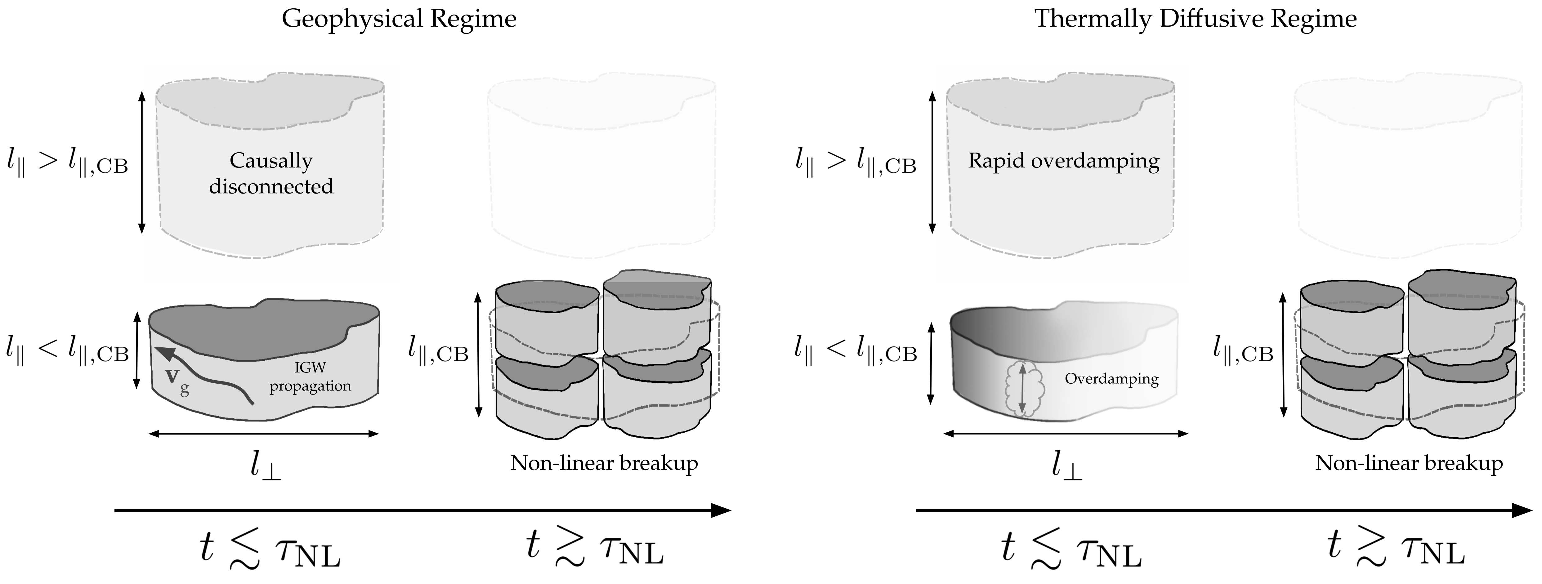
Figure 2: A sketch of the physical arguments used for critical balance for eddies with perpendicular extent $l_{\perp}\sim k_{\perp}^{-1}$. The notation $l_{\parallel,\rm CB}$ refers to the $l_{\parallel}\sim k_{\parallel}^{-1}$ that satisfies critical balance in each regime. The left side shows the causality argument for the geophysical regime ($PrRb>1$). Since the group velocity, $\textbf{v}_{\rm g}$, of the associated IGW sets the speed at which information can propagate, any eddy with $l_{\parallel}>l_{\parallel,\rm CB}$ would be causally disconnected before it non-linearly breaks up within time $t\sim\tau_{\rm NL}$. The right side shows the selective decay argument for the thermally diffusive regime ($PrRb<1$). Since the damping rate increases with $\gamma_{\rm lPe}\sim l_{\parallel}^{4}$, any eddy with $l_{\parallel}>l_{\parallel,\rm CB}$ would rapidly decay away before it could evolve.

In the limit $PrRb\ll 1$ ($l_{\kappa}\gg l_{O}$), thermal diffusion is faster than the restoring buoyancy timescale so $\gamma_{\kappa}\gg\omega_{\mathrm{N}}$ and the two roots of Eq 9 become $\omega\sim i\omega^{2}_{N}/\gamma_{\kappa}$ and $\omega\sim i\gamma_{\kappa}$. The latter is an uninteresting rapid thermal diffusion rate, while the former is an effective damping rate $\omega_{\mathrm{lPe}}=i\omega^{2}_{N}/\gamma_{\kappa}=iN^{2}k_{\perp}^{2}/\kappa k^{4}$ (lignieres1999small; lignieres2019turbulence). Thus, the linear response frequency is no longer a real frequency of a restoring oscillation, but instead a damping rate $\gamma_{\mathrm{lPe}}$ $(\omega_{\mathrm{lPe}}=i\gamma_{\mathrm{lPe}})$ corresponding to the effective rate that restoring buoyancy and strong thermal diffusion operate on. A direct linear analysis of the low turbulent Peclet equations (Eq 3) also gives the eponymous damping rate $\omega=i\gamma_{\mathrm{lPe}}$—the two approaches nicely agree. Using the expectation of strong anisotropy at large scales $k_{\perp}/k_{\parallel}\ll 1$, the linear damping timescale can be estimated as:

$$\gamma_{\mathrm{lPe}}\sim\frac{N^{2}k_{\perp}^{2}}{\kappa k_{\parallel}^{4}}$$ (10)

Before the critical balance hypothesis can be applied, a new justification is needed because the causality argument in the $PrRb>1$ regime no longer applies: waves are overdamped rather than propagate. The instantaneous propagation of information is a peculiarity of the low Peclet equations (Eqs 3) since the temperature and vertical velocity fields are coupled by an elliptic equation to lowest order. Critical balance instead becomes an argument for selective decay. The dependence between the damping rate of a fluctuation and its vertical extent $\gamma_{\rm lPe}\sim l_{\parallel}^{4}$ according to Eq 10 means that longer vertical structures overdamp faster. As a result, any fluctuation at some $k_{\perp}$ with parallel extent longer than the $l_{\parallel}\sim k_{\parallel}^{-1}$ set by $\gamma_{\rm lPe}\tau_{\rm NL}\sim 1$ will rapidly decay away before non-linear effects can become significant. Critical balance in the thermally diffusive regime thus determines the longest parallel structure for a given $k_{\perp}$ that can sustain before non-linear breakup. A sketch of the physical argument is shown in Figure 2, alongside a comparison with the causality argument in the $PrRb>1$ regime.

With the modified physical interpretation, application of critical balance $\gamma_{\mathrm{lPe}}\tau_{\mathrm{NL}}\sim 1$ and rearrangement gives the new relationship between $k_{\perp}$ and $k_{\parallel}$:

$$\frac{k_{\perp}}{k_{\parallel}}\sim\left(\frac{\kappa\epsilon^{1/3}}{N^{2}}\right)^{3/4}k^{2}_{\parallel}=l_{OM}^{2}k_{\parallel}^{2}$$ (11)

where the modified Ozmidov scale is defined as $l_{OM}=(\kappa\epsilon^{1/3}/N^{2})^{3/8}$. One can check that the critical balance prediction self-consistently maintains $\omega_{\mathrm{N}}/\gamma_{\kappa}\ll 1$ all the way to the largest scales since $\omega_{\mathrm{N}}/\gamma_{\kappa}\sim Nk_{\perp}/\kappa k_{\parallel}^{3}\sim(PrRb)^{1/4}\ll 1$. The turbulence now returns to isotropy at the modified Ozmidov scale where the overdamping rate for a fluctuation with $k_{\perp}\sim k_{\parallel}$ is comparable to its eddy turnover time $N^{2}l_{\rm OM}^{2}/\kappa\sim\tau_{\rm NL}^{-1}$. In analogy to the Ozmidov scale, the modified Ozmidov scale is the largest horizontal scale that can overturn before overdamping becomes significant. Note that the modified Ozmidov is larger than the Ozmidov scale as would be expected:

$$l_{OM}=\frac{Fr^{3/2}}{(PrRb)^{3/8}}L,\quad\frac{l_{OM}}{l_{O}}=(PrRb)^{-3/8}>1$$ (12)

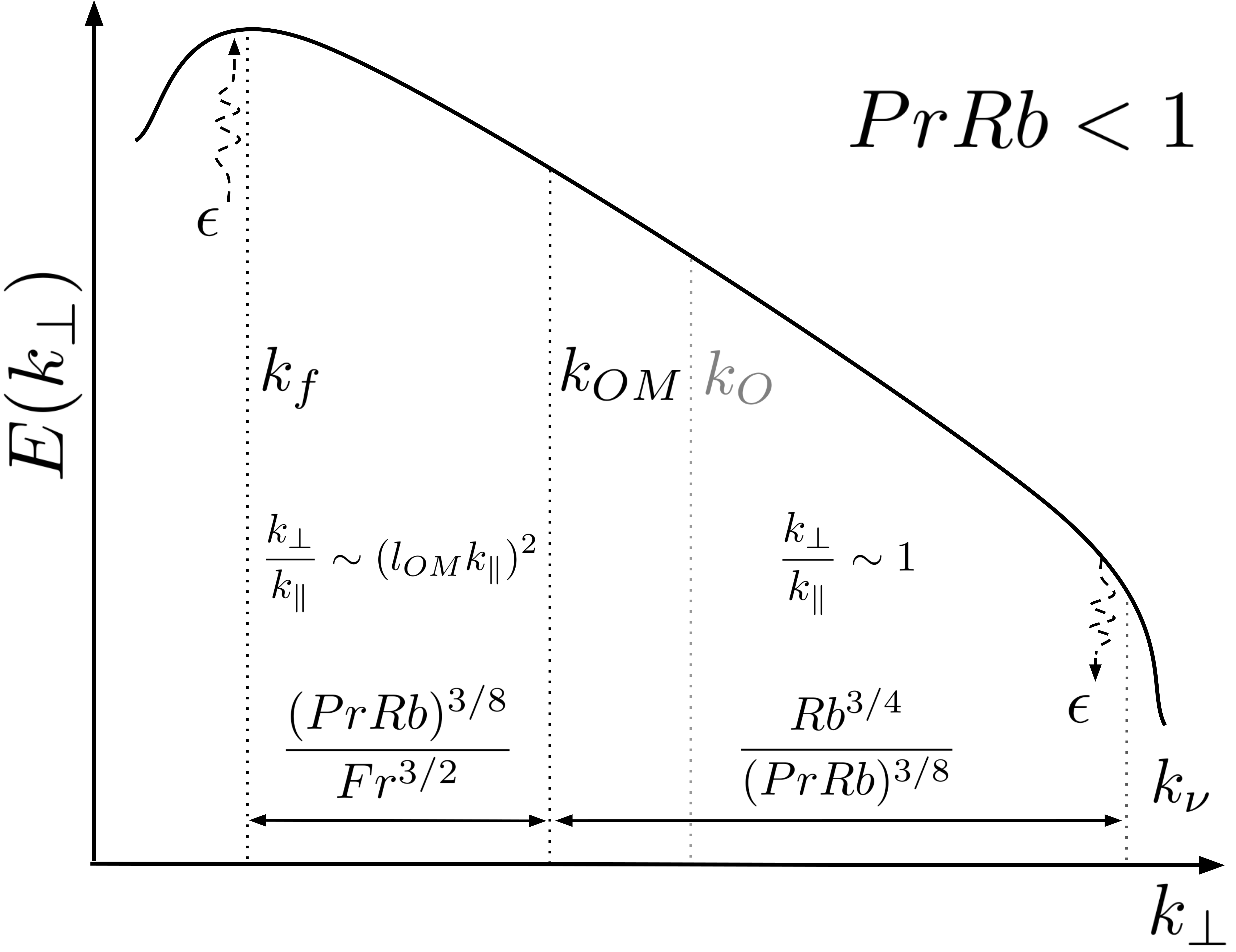
Figure 3: Energy cascade for strongly stratified turbulence for $PrRb\ll 1$ relevant to the $Pr\ll 1$ regime of stellar radiative zones. Similar to Figure 1, an anisotropic cascade results in the range $k_{f}\lesssim k_{\perp}\lesssim k_{OM}$ followed by an isotropic cascade from $k_{OM}$ to $k_{\nu}$. Note that the beginning of the isotropic subrange has moved to larger scales $k_{OM}<k_{O}$.

The outer vertical scale ($k_{\parallel}\sim l_{z}^{-1}$) at the largest horizontal scale where $k_{\perp}\sim L^{-1}$ can again be found. Subsequent enforcement of incompressibility $(\nabla\cdot\textbf{u}^{\prime}=0)$ then gives $u_{z}\sim l_{z}U/L$. The result is shown below:

$$l_{z}\sim\frac{Fr}{(PrRb)^{1/4}}L,\quad u_{z}\sim\frac{Fr}{(PrRb)^{1/4}}U.$$ (13)

These scalings self-consistently predict a small turbulent Peclet number $Pe_{t}\sim(PrRb)^{1/2}\ll 1$. At this point it becomes suggestive to define a modified Froude number as $Fr_{M}\equiv Fr/(PrRb)^{1/4}$ so that:

$$l_{z}=Fr_{M}L,\quad l_{OM}=Fr_{M}^{3/2}L.$$ (14)

These are the same exponents as in the geophysical regime. Using the new definition, the corresponding horizontal and vertical spectra for $k<k_{OM}$ are:

$$\frac{E(k_{\perp})}{U^{2}L}\sim(k_{\perp}L)^{-5/3},\quad\frac{E(k_{\parallel})}{U^{2}L}\sim Fr_{M}(k_{\parallel}l_{z})^{-3}$$ (15)

The dimensional form of the parallel energy spectrum $E(k_{\parallel})\sim N(\epsilon/\kappa)^{1/2}k_{\parallel}^{-3}$ now depends on the dissipation and thermal diffusivity, unlike in the geophysical regime where $E(k_{\parallel})\sim N^{2}k_{\parallel}^{-3}$. A schematic of the energy cascade is shown in Figure 3 and a comparison of the cascade path in the $k_{\perp}-k_{\parallel}$ plane with the $PrRb>1$ regime is shown in Figure 4.

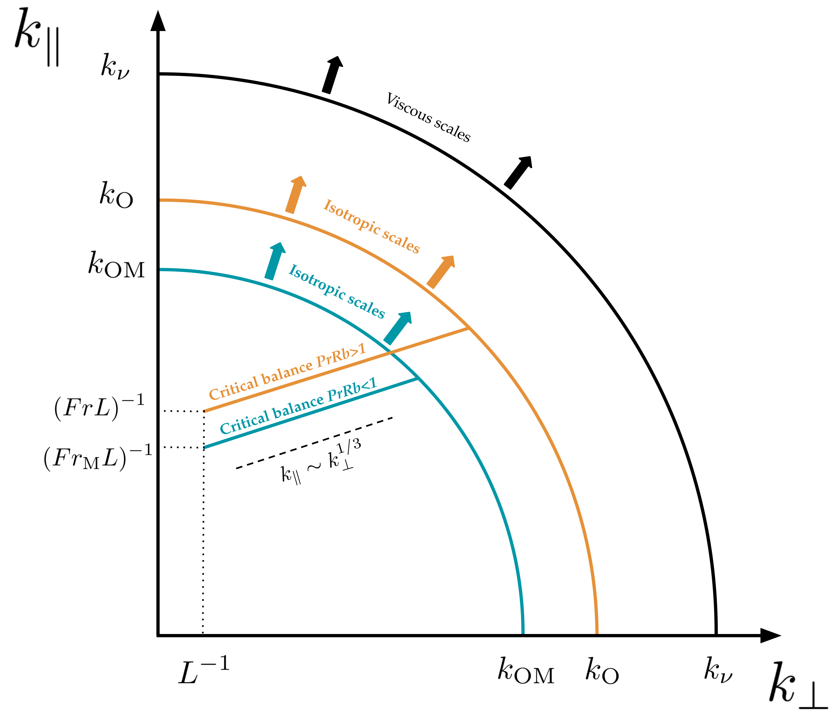
Figure 4: Comparison of the cascade path in the $k_{\perp}-k_{\parallel}$ plane between the geophysical (teal) and thermally diffusive (orange) regimes. Energy is injected at low perpendicular wavenumber $k_{\perp}\sim L^{-1}$, follows the critical balance path until the respective Ozmidov scale ($k_{\rm O}$ or $k_{\rm OM}$), enters the isotropic cascade, and then is dissipated at the viscous scales.

It is now clear that the transition from the $PrRb>1$ to the $PrRb<1$ regime simply corresponds to a replacement $Fr\rightarrow Fr_{M}$. How can this modified Froude number be physically understood? If the Froude number is reinterpreted to define the ratio of the emergent vertical length scale to the imposed horizontal scale (i.e. $l_{z}/L\equiv Fr$), then critical balance at the largest scales simply sets the Froude number. By substituting $k_{\perp}\sim L^{-1}$ and $k_{\parallel}\sim l_{z}^{-1}$ into the linear wave frequencies $\omega_{\mathrm{N}}\sim Nl_{z}/L$ and $\gamma_{\mathrm{lPe}}\sim N^{2}l_{z}^{4}/\kappa L^{2}$ and then comparing both with the corresponding non-linear frequency scale $\tau_{\mathrm{NL}}^{-1}\sim U/L$, the two Froude numbers emerge: PrRb¿1&: lzL∼ULN≡Fr,
PrRb¡1: lzL∼(κUN2L3)^1/4≡Fr_M.

As should be expected, the outer vertical scales smoothly transition from $l_{z}/L=Fr$ to $l_{z}/L=Fr/(PrRb)^{1/4}$ at $PrRb=1$ when $Pr$ is decreased. This is analogous to the smooth transition from $l_{z}/L=Fr$ to $l_{z}/L=Fr/(Rb)^{1/2}$ at $Rb=1$ when $Re$ is decreased, as discussed in Section 2.3. Additionally, we note that $Fr_{M}$ can be rewritten in terms of $PeFr^{-2}$ and $Re$ (i.e. $Fr_{M}=(PeFr^{-2})^{-1/4}$) as was required by the low turbulent Peclet approximation.

With the acquired scaling relations from critical balance above, we suggest the following dimensionalization for rescaling the Boussinesq equations in the $PrRb\ll 1$ limit:

u_h’=U u_h, u_z’=Fr_MUu_z, θ’=1FrMU2Lθ, p’= ρ_m U^2p,
x’=Lx, y’=L y, z’=Fr_ML z, t’=LU t, Aside from $z^{\prime}$ and $u_{z}^{\prime}$, the only other variable whose scaling changed is $\theta^{\prime}$, which is now determined by the new dominant balance between $N^{2}u_{z}^{\prime}\sim\kappa\nabla_{z}^{2}\theta^{\prime}$ as discussed in Section 2.3. The Boussinesq equations become:

∂_t u_h+u⋅∇u_h&=-∇_h p+ [1Re∇_h^2+1RbM∇_z^2]u_h,
Fr_M^2[∂_t u_z+u⋅∇u_z]=-∇_z p+θ+Fr_M^2[1Re∇_h^2+1RbM∇_z^2]u_z,
(PrRb)^1/2[∂_tθ+u⋅∇θ]=-u_z+ [(PrRb)1/2PrRe∇_h^2+∇_z^2]θ,
∇⋅u=0,

We see that $Rb_{M}\equiv ReFr_{M}^{2}=Rb/(PrRb)^{1/2}$ acts as the new effective Reynolds number and nicely matches with the scale separation between the modified Ozmidov and the viscous scale $l_{OM}/l_{\nu}=(Rb_{M})^{3/4}$. To lowest order:

∂_t u_h+u⋅∇u_h&=-∇_h p,
0=-∇_z p+θ,
0=-u_z+∇_z