Bratteli diagrams, translation flows and their $C^{*}$-algebras

Abstract.

In [LT16], Kathryn Lindsey and the second author constructed a translation surface from a bi-infinite Bratteli diagram. We continue an investigation into these surfaces. The construction given in [LT16] was essentially combinatorial. Here, we provide explicit links between the path space of the Bratteli diagram and the surface, including various intermediate topological spaces. This allows us to relate the $C^{*}$-algebras associated with left and right tail equivalence on the Bratteli diagram and the vertical and horizontal foliations of the surface, under some mild hypotheses. This also allows us to relate the K-theory of the $C^{*}$-algebras involved. We also treat the case of finite genus surfaces in some detail, where the process of Rauzy-Veech induction (and its inverse) provide an explicit construction of the Bratteli diagrams involved.

1. Introduction

There has been considerable interest over many years in the dynamics of foliations and flows on translation surfaces or flat surfaces. We refer the reader to [Via06, Zor06, FM14] for a broader discussion.

In [LT16], Kathryn Lindsey and the second author introduced a construction of translation surfaces based on combinatorial data. The main point of the construction was that, while giving an alternate view of the finite genus case, it also provided a very general method of construction of surfaces of infinite genus. In addition, it was shown that the dynamical behavior on these infinite genus surfaces was much broader than the finite genus case.

The combinatorial data needed for the construction is a variation of a Bratteli diagram. A Bratteli diagram is a locally finite, but infinite directed graph. They first appeared in Ola Bratteli’s seminal work on inductive limits of finite dimensional $C^{*}$-algebras, or AF-algebras [Bra72]. Bratteli used the diagrams to encode combinatorial data on maps between direct sums of matrix algebras. Later, Renault [Ren80] showed that the diagrams could also be used to construct topological groupoids (equivalence relations) and the $C^{*}$-algebras constructed from such examples coincided with those considered by Bratteli. More specifically, one considers the topological space of infinite paths in the diagram along with the equivalence relation known as tail equivalence: two paths are tail equivalent if they are equal beyond some fixed point.

More recently, Bratteli diagrams also been used extensively in dynamical systems, initiated by the work of Vershik [Ver82, Ver95] and subsequently, Herman, Putnam and Skau [HPS92]. In particular, this involved introducing the notion of an ordered Bratteli diagram.

Bratteli diagrams were first used in the context of the dynamics of translation surfaces by A. Bufetov [Buf14]. This was expanded upon by K. Lindsey and the second author [LT16]. Their innovation was to consider a bi-infinite Bratteli diagram, where the vertex and edge sets are indexed by the integers, rather than the positive integers as is usually the case. They also assume a pair of orders on the edge set the first compares edges having the same range or terminus and the second compares edges having the same source or origin.

The construction of the surface was then given in [LT16] in a combinatorial manner: finite paths gave open rectangular components for the surface and the terminus, origin and order data provides rules for attaching them. One also sees that the leaves of the horizontal and vertical folitations correspond to right and left tail equivalence in the diagram. From a dynamical standpoint that is quite satisfactory, but it leaves open the question: if we think about the AF-algebra of the diagram and the foliation $C^{*}$-algebra, how exactly are they related? The main goal of this paper is to address this question.

On the one hand, we have a very satisfactory description of the AF-algebra as given by Renault, by looking at the path space of the diagram, tail equivalence on it, and the standard construction of a groupoid $C^{*}$-algebra. What is missing on the other side is a description of the surface itself in terms of the infinite path space of the diagram. At first glance, this seems a tall order because the former is a locally Euclidean space while the latter is totally disconnected. A good clue that these are not so far apart is provided by a very familiar, but under-appreciated, notion: decimal expansion. This is already a familiar idea in dynamics through the use of Markov partitions to code hyperbolic systems. Let us take some time to describe this simple idea more clearly as it is essentially the basis for the remainder of the paper.

Everyone is familiar with the fact that every real number has a decimal expansion which is (almost) unique. A more mathematically precise view of decimal expansion is as a map from $\prod_{1}^{\infty}\{0,1,2,\ldots,9\}$ to $[0,1]$ (simply ignoring the integer part). It is surjective and each point in the image has a unique pre-image, except a countable subset: rational numbers of the form $k/10^{l},k\in\mathbb{Z},l\geq 1$.

This becomes more interesting if the first space is given the product topology. The map is then continuous, but the two spaces are remarkably different: the first is totally disconnected, while the second is connected.

Another viewpoint is to realize that the first space can be endowed with lexicographic order. The order topology coincides with the product topology and the map is order preserving. In fact, more is true: if we note, for example, that $.19999\cdots$ and $.2000\cdots$ are both decimal expansions of $\frac{1}{5}$, the latter is precisely the successor of the former in the lexicographic order. In fact, two points are identified by the map if and only if one is the successor of the other.

Bratteli diagrams offer a vast generalization of this idea. A Bratteli diagram, $\mathcal{B}$, consists of a sequence of finite non-empty vertex sets $V_{n},n\geq 0$ (we assume $\#V_{0}=1$ for convenience) and edge sets $E_{n},n\geq 1$: each edge $e$ in $E_{n}$ has a source $s(e)$ in $V_{n-1}$ and a range $r(e)$ in $V_{n}$. We can then consider the space of infinite paths, denoted $X_{\mathcal{B}}$. It has natural topology making it compact and totally disconnected. We add two pieces of data: a state $\nu$ (see Definition 2.6 and a partial order on the edge sets where two edges, $e,f$, are comparable if and only if $s(e)=s(f)$. Such items always exist. The path space $X_{\mathcal{B}}$ then becomes linearly ordered by lexicographic order. In addition, the state provides a measure on this space in a natural way (3.7). We can then define explicitly a map from $X_{\mathcal{B}}$ to a closed interval which is order-preserving and identifies two points if and only if one is the successor of the other. We leave the details to Lemma 4.3. Usual decimal expansion can be seen in the case $\#V_{n}=1,\#E_{n}=10$, for all $n\geq 1$.

This is appealing, though not terribly deep. The Lindsey-Treviño starting point is to consider a bi-infinite Bratteli diagram where the vertex and edge sets are indexed by the integers rather than the natural numbers. We drop the condition that $\#V_{0}=1$. In addition, we require two orders on the edge sets, one based on $s$ (as before) and the other on $r$ and two states, $\nu_{s},\nu_{r}$. Our path space $X_{\mathcal{B}}$ now consists of bi-infinite paths. Basically, our surface is now obtained as a quotient of $X_{\mathcal{B}}$ by identifying successor/predecessors in both orders. That is overly simplistic and we need to make some subtle alterations. But let us leave that aside for the moment and describe this space, locally. If we fix a finite path $p$ in the diagram going from vertex $v$ in $V_{m}$ to $w$ in $V_{n}$, $m<n$, we can look at the set of all bi-infinite paths which agree with $p$ between $m$ and $n$. This is a clopen set. But it is clear that such a path consists of three parts, from $-\infty$ to $s(p)$, then $p$, then from $r(p)$ to $\infty$. The first and third parts are clearly independent and lie in the path spaces of two subdiagrams (although the first is oriented the wrong direction). Applying the map we described earlier using the $r$-data to the first and the $s$-data to the third, we obtain a map to a closed rectangle in the plane which descends to a local homeomorphism on our quotient space. These maps can be used to define an atlas for the quotient space which satisfy the condition making it a translation surface. Moreover, if two points are right-tail equivalent then they lie on the same horizontal line, while two points that are left-tail equivalent lie on the same vertical line. So our quotient map from $X_{\mathcal{B}}$ to the surface maps right-tail equivalence to the horizontal foliation and left-tail equivalence to the vertical foliation. This provides the links between the AF-algebras and the foliation algebras which is our main goal.

In section 2, we describe basics of Bratteli diagrams. In particular, we have the classic version, the bi-infinite version and ordered versions of both. This includes some basic concepts such as a simple diagram (2.4) (some telescope has full edge connections) and finite rank (2.5), which means that there is a uniform bound on the cardinality of the vertex sets. The third section describes the path space of a Bratteli diagram, both classic and bi-infinite versions. In the fourth section, we describe the consequences for the infinite path space of orders on a Bratteli diagram. This includes a complete description of the analogues of decimal expansion as discussed above.

As we indicated above, our basic idea is to begin with a bi-infinite ordered Bratteli diagram, $\mathcal{B}$, and take a quotient of the path space of a bi-infinite Bratteli diagram, $X_{\mathcal{B}}$. However, there are some bad points in this space that need to be dealt with, just as flat surfaces in genus greater than one necessarily have singularities. These fall into two types. The first are those in which every path is maximal in the $\leq_{s}$-order or maximal in the $\leq_{r}$-order or minimal in the $\leq_{s}$-order or minimal in the $\leq_{r}$-order. We refer to these are extremal (5.1) and, if the diagram is finite rank, it is a finite set. More subtly, there is a second type of point, which we call singular. We have two (partially defined) operations: taking the successor in the $\leq_{s}$-order and taking the successor in the $\leq_{r}$-order. There may be points where their compositions are defined, in either order, but fail to yield the same result. This is our ordered Bratteli diagram’s way of telling us the common point they represent in the quotient space will fail to have a flat neighourhood. These points, which we denote by $\Sigma_{\mathcal{B}}$, must be removed (5.1). The set is, at worst countable, and its union with the extremal points is closed. We now restrict our attention to the open compliment of this, which we denote by $Y_{\mathcal{B}}$ 6.1.

In section 6, we introduce our surface, $S_{\mathcal{B}}$. This is done by identifying points of $Y_{\mathcal{B}}$ with their $\leq_{s}$-successors and their $\leq_{r}$-successors. Of course, this means that there are two intermediary spaces where only one of the two identifications is done. The main work of this section is to explicitly describe an atlas for the space $S_{\mathcal{B}}$ whose transition maps are translations. That is, we show $S_{\mathcal{B}}$ is a flat surface. It is worth noting that $S_{\mathcal{B}}$ depends only on the ordered Bratteli diagram, but the atlas also depends on the given state.

In section 7, we pass from the various spaces of the previous section, to groupoids associated with them. While we use the term groupoid, these are really simply equivalence relations. For the bi-infinite path space $X_{\mathcal{B}}$ or its open subset $Y_{\mathcal{B}}$, we have right and left tail equivalence. For the surface, $S_{\mathcal{B}}$, we have horizontal and vertical foliations. The process of constructing a $C^{*}$-algebra from a groupoid is technical; in particular, the groupoid requires its own topology. We describe all of these in quite concrete terms. Finally, our maps between the various spaces of section 6 all induce maps at the level of equivalence relations and we describe their properties. Indeed, one of the quotient maps from $Y_{\mathcal{B}}$ does not respect tail equivalence in general and we are forced to make a small modification of it in Definition 7.5.

We turn to the $C^{*}$-algebras in section 8. We explicitly show how the $C^{*}$-algebras of tail equivalence can be written as inductive limits of a nested sequence of finite-dimensional subalgebras. In the case of one of the intermediate subalgebras, we also have an inductive system 8.9 and 8.10 of subalgebras which are ’subhomogeneous’. That is, they involve only continuous functions from certain spaces into matrices. The same also holds for the foliation algebra.

In section 9, we construct a very natural Fredholm module for our AF-algebra. The notion of a Fredholm module for $C^{*}$-algebras had its origins in the seminal work of Brown, Douglas and Fillmore on extensions of $C^{*}$-algebras but also from index theory through ideas of Atiyah and Kasparov, among many others. There are many good references but we mention the three books by Blackadar [Bla86], Higson and Roe [HR01] and Connes [Con94]. The prototype here is the $C^{*}$-algebra of continuous functions on a smooth manifold together with an elliptic differential operator (or a bounded version of it). The algebra and operator interact in a special way. In our situation, our Fredholm module provides a purely algebraic way of describing our quotient spaces (see Theorem 9.6). This description, in turn, is critical to some K-theory computations of the next section.

We describe the K-theory of the various $C^{*}$-algebras involved in section 10, beginning with the AF-algebra. The computation of the K-theory of an AF-algebra from a Bratteli diagram goes back to Elliott’s seminal paper [Ell76], but we give a treatment in some detail for those readers for whom this is new. We also compute the K-theory of one intermediate $C^{*}$-algebra in generality in Theorem 10.4. In many specific situations of interest, this $C^{*}$-algebra has $K_{1}$ equal to the integers, while its inclusion in the AF-algebra induces and order isomorphism om $K_{0}$ (see Theorem 10.5). We go on to compute the K-theory of the foliation algebra in Theorems 10.7 and 10.9. One interesting conclusion of these computations is that, when the Bratteli diagram has finite rank, the $K_{0}$ group of the AF-algebra does also, in the sense of group theory. However, if that group is not finitely-generated, then our surface has infinite genus (Corollary 10.11).

We end the paper with two sections in which we apply the tools developed so far: in section 11 we work out the $K$-theory of the horizontal foliation of Chamanara’s surface. Chamanara’s surface is perhaps the best known flat surface of infinite genus and finite area. In particular, we show how one can explicitly construct representatives of certain $K_{0}$ classes coming from the surface.

Section 12 deals with flat surfaces of finite genus. Starting with basic definitions of flat surfaces, we review Veech’s construction of zippered rectangles and Rauzy-Veech (RV) induction, which is a procedure used in the renormalization of the vertical foliation of a flat surface. We follow this by developing an analogous induction procedure for the horizontal foliation, which we call RH induction. This is formally the inverse of RV induction, but we motivate it geometrically and develop it independently of RV induction. As far as we know a lot of this has not been published before, although many items appear in the recent work of Berk [Ber21]. The reason we focus on the induction for the horizontal foliation is that it turns out to give an ordered bi-infinite Bratteli diagram which is simpler to analyse. We compute the $K$-theory of the foliation algebra of the horizontal foliation of the typical flat surface of finite genus. We also show that the order structure on the $K_{0}$ groups is defined by the Schwartzman asymptotic cycle.

Acknowledgements: R.T. was partially supported by NSF grant 1665100 and Simons Collaboration Grant 712227. I.F.P. was supported by a Discovery Grant from NSERC (Canada).

2. Bratteli diagrams: ordered and bi-infinite

In this section, we discuss the notion of a Bratteli diagram. This is a fairly well-known combinatorial object, but we will need to discuss a bi-infinite variation and also the notion of orders on both types.

Definition 2.1.

A Bratteli diagram is two sequences $V_{n},n\geq 0,E_{n},n\geq 1$ of pairwise disjoint, finite, nonempty sets along with surjective maps $r:E_{n}\rightarrow V_{n}$ and $s:E_{n}\rightarrow V_{n-1}$ for $n\geq 1$. We also assume that $V_{0}$ consists of a single element we write as $v_{0}$. We write $V$ for the union of the $V_{n}$ and $E$ for the union of the $E_{n}$. We also write $\mathcal{B}=(V,E,r,s)$.

Definition 2.2.

A bi-infinite Bratteli diagram is two sequences $V_{n},E_{n},n\in\mathbb{Z}$ of pairwise disjoint, finite, nonempty sets (dropping the requirement that $\#V_{0}=1$) along with surjective maps $r:E_{n}\rightarrow V_{n}$ and $s:E_{n}\rightarrow V_{n-1}$. We write $V$ for the union of the $V_{n}$ and $E$ for the union of the $E_{n}$. We also write $\mathcal{B}=(V,E,r,s)$.

A standard convention when drawing in drawing Bratteli diagrams is to draw them vertically, with $v_{0}$ at the top of the diagram and level $V_{n+1}$ drawn below $V_{n}$. Here, we prefer to draw them horizontally. That is, $V_{n+1}$ lies to the right of $V_{n}$, as shown below. For ordinary Bratteli diagrams, this change is rather minor, but it seems helpful when considering bi-infinite ones, not to have to imagine the diagram extending off the top of page.

Definition 2.3.

If $\mathcal{B}$ is a bi-infinite Bratteli diagram, for every pair of integers $m<n$, we let $E_{m,n}$ be the set of all paths from $V_{m}$ to $V_{n}$: that is, it consists of $p=(p_{i})_{m<i\leq n}$ with $p_{i}$ in $E_{i}$, $m<i\leq n$, and $r(p_{i})=s(p_{i+1})$, for $m<i<n$. We define $r:E_{m,n}\rightarrow V_{n}$ by $r(p)=r(p_{n})$ and $s:E_{m,n}\rightarrow V_{m}$ by $s(p)=s(p_{m+1})$. We make the same definition if $\mathcal{B}$ is a Bratteli diagram, restricting to $0\leq m<n$.

We note the fairly standard notion of simplicity of a Bratteli diagram and its obvious extension to the bi-infinite case.

Definition 2.4.

1. A Bratteli diagram $\mathcal{B}$ is simple if and only if, for every $m\geq 1$, there is $n>m$ such that for every vertex $v$ in $V_{m}$ and $w$ in $V_{n}$, there is a path $p$ in $E_{m,n}$ with $s(p)=v,r(p)=w$.

2. A bi-infinite Bratteli diagram $\mathcal{B}$ is $\mathcal{B}$ is simple if, for every integer $m$, there are integers $l<m<n$ such that there is a path from every vertex of $V_{l}$ to every vertex of $V_{m}$ and there is a path from every vertex of $V_{m}$ to every vertex of $V_{n}$.

We also introduce the following notion which will be convenient for much of what follows.

Definition 2.5.

A Bratteli diagram (or bi-infinite Bratteli diagram) is finite rank if there is a constant $K$ such that $\#V_{n}\leq K$, for all $n\geq 0$ (or all $n\in\mathbb{Z}$, respectively).

We next discuss the notion of a state on a Bratteli diagram, and its analogue for the bi-infinite case. We add as a small remark that it is usual to begin with a Bratteli diagram and consider the set of all possible states on it. For our applications later, we will usually think of a Bratteli diagram, together with a fixed state, as our data.

Definition 2.6.

1. Let $\mathcal{B}$ be a Bratteli diagram. A state on $\mathcal{B}$ is a function $\nu_{s}:V\rightarrow[0,\infty)$ satisfying

   $$\nu_{s}(v)=\sum_{s(e)=v}\nu_{s}(r(e)),$$

   for all $v$ in $V$. We say that the state is normalized if $\nu_{s}(v_{0})=1$ and faithful if $\nu_{s}(v)>0$, for all $v$ in $V$. We let $S(\mathcal{B})$ be the set of all states on $\mathcal{B}$ and $S_{1}(\mathcal{B})$ denote the set of normalized states.

2. Let $\mathcal{B}$ be a bi-infinite Bratteli diagram. A state on $\mathcal{B}$ is a pair of functions $\nu_{r},\nu_{s}:V\rightarrow[0,\infty)$ satisfying

   $$\nu_{r}(v) = \sum_{r(e)=v}\nu_{r}(s(e)),$$

   $$\nu_{s}(v) = \sum_{s(e)=v}\nu_{s}(r(e)),$$

   for all $v$ in $V$. We say that the state is normalized if

   $$\sum_{v\in V_{0}}\nu_{r}(v)\nu_{s}(v)=1$$

   and is faithful if $\nu_{r}(v),\nu_{s}(v)>0$, for all $v$ in $V$. We let $S(\mathcal{B})$ be the set of all states on $\mathcal{B}$ and $S_{1}(\mathcal{B})$ denote the set of normalized states.

Lemma 2.7.

If $\nu_{r},\nu_{s}$ is a state on bi-infinite Bratteli diagram, $\mathcal{B}$, then

$$\sum_{v\in V_{n}}\nu_{r}(v)\nu_{s}(v)=\sum_{v\in V_{0}}\nu_{r}(v)\nu_{s}(v)$$

for every integer $n$.

Proof.

If $n$ is any integer, we have

$$\sum_{v\in V_{n}}\nu_{r}(v)\nu_{s}(v) = \sum_{v\in V_{n}}\nu_{r}(v)\sum_{s(e)=v}\nu_{s}(r(e))$$

$$= \sum_{v\in V_{n}}\sum_{s(e)=v}\nu_{r}(v)\nu_{s}(r(e))$$

$$= \sum_{e\in E_{n+1}}\nu_{r}(s(e))\nu_{s}(r(e))$$

$$= \sum_{v\in V_{n+1}}\sum_{r(e)=v}\nu_{r}(s(e))\nu_{s}(v)$$

$$= \sum_{v\in V_{n+1}}\nu_{r}(v)\nu_{s}(v).$$

The conclusion follows. ∎

Let us remind the reader that the computation of the set of states for a one-sided Bratteli diagram is a standard result, which can be easily adapted to the bi-infinite case. It is convenient to assume that $V_{n}=\{n\}\times\{1,2,\ldots,d_{n}\}$, for all integers $n$. Without causing confusion, we can interpret $E_{n}$ as a $d_{n}\times d_{n-1}$ non-negative integer matrix whose $j,i$-entry is the number of edges in $E_{n}$ from $(n-1,i)$ in $V_{n-1}$ to $(n,j)$ in $V_{n}$. In the following, we let $\mathbb{R}^{+m}$ denote vectors in $\mathbb{R}^{m},m\geq 1$, whose entries are all non-negative.

Proposition 2.8.

Let $\mathcal{B}$ be a bi-infinite Bratteli diagram. If $\nu_{r},\nu_{s}$ is a state on $\mathcal{B}$, then for all integers $n$, we have

$$\left(\nu_{s}(n,i)\right)_{i=1}^{d_{n}} \in\displaystyle\bigcap_{m>n}\mathbb{R}^{+d_{m}}E_{m}E_{m+1}\cdots E_{n+1}, 1\leq i\leq d_{n},$$

$$\left(\nu_{r}(n,i)\right)_{i=1}^{d_{n}} \in\displaystyle\bigcap_{m<n}\mathbb{R}^{+d_{m}}E_{m+1}^{T}E_{m+2}^{T}\cdots E_{n}^{T}, 1\leq i\leq d_{n}.$$

Conversely, letting $\Delta^{d-1}$ denote the standard $d-1$-simplex in $\mathbb{R}^{+d}$, the sets

$$\displaystyle\bigcap_{m>0}\mathbb{R}^{+d_{m}}E_{m}E_{m+1}\cdots E_{n+1} \cap \Delta^{d_{0}-1}$$

$$\displaystyle\bigcap_{m>0}\mathbb{R}^{+d_{m}}E_{m+1}^{T}E_{m+2}^{T}\cdots E_{n}^{T} \cap \Delta^{d_{0}-1}$$

are non-empty. Let $x^{0}$ be in the former and set $\nu_{s}(0,i)=x_{i}^{0},1\leq i\leq d_{0}$, $\nu_{s}(n,i)=(xE_{-1}^{T}E_{-2}^{T}\cdots E_{n}^{T})_{i}$, for $n<0,1\leq i\leq d_{n}$. Finally, for each $n>0$, inductively find $x^{n}$ in $\mathbb{R}^{+d_{n}}$ with $x^{n}=x^{n-1}E_{n}$ and set $\nu_{s}(n,i)=x_{i}^{n},1\leq i\leq d_{n}$. We may also define $\nu_{r}$ in an analogous way and $\nu_{s},\nu_{r}$ is a state on $\mathcal{B}$.

Proposition 2.9.

Let $\mathcal{B}$ be a bi-infinite Bratteli diagram.

1. $S(\mathcal{B})$ is non-empty.

2. If $\mathcal{B}$ is simple, then every state is faithful.

Proof.

For the second part, the following are easy consequences of the definition:

1. If there is a vertex $v$ in $V_{n}$ such that $\nu_{r}(v)>0$, then there exists a vertex $w$ in $V_{n-1}$ such that $\nu_{r}(v)>0$.

2. If $m<n$ is such that there is a path from every vertex in $V_{m}$ to every vertex in $V_{n}$, and there is there is a vertex $v$ in $V_{m}$ such that $\nu_{r}(v)>0$, then for every vertex $w$ in $V_{n-1}$, $\nu_{r}(v)>0$.

   Now let $n$ be an integer. By Lemma 2.7, there is some $v$ in $V_{n}$ such that $\nu_{r}(v)>0$. Next, choose $m<n$ such that $E_{m,n}$ has full connections. It follows from the first point above that there exists $w$ in $V_{m}$ such that $\nu_{r}(w)>0$. It then follows from the second point above that $\nu_{r}(v^{\prime})>0$, for all $v^{\prime}$ in $V_{n}$. As $n$ was arbitrary, this completes the proof.

∎

We will ultimately be interested in ordered bi-infinite Bratteli diagrams. We make the definition now, although we will not make use of it until section 4.

Definition 2.10.

A bi-infinite, ordered Bratteli diagram is a bi-infinite Bratteli diagram, $\mathcal{B}=(V,E,r,s)$, along with partial orders $\leq_{s},\leq_{r}$ on $E$ such that, for any $e,f$ in $E$, they are $\leq_{s}$-comparable if and only if $s(e)=s(f)$, and are $\leq_{r}$-comparable if and only if $r(e)=r(f)$. We write $\mathcal{B}=(V,E,r,s,\leq_{r},\leq_{s})$.

We adopt the following obvious notation: $e<_{r}f$ (respectively, $e<_{s}f$) if and only if $e\leq_{r}f$ ($e\leq_{s}f$) and $e\neq f$.

The definition of the orders can also be extended to $E_{m,n}$ using the lexicographic order carefully noting that $\leq_{r}$ works right-to-left while $\leq_{s}$ works left-to-right.

If $e$ is any edge in $E$, we let $S_{s}(e)$ be its $\leq_{s}$-successor, provided it exists. Similar, $P_{s}(e)$ denotes its $\leq_{s}$-predecessor. There are analogous definitions of $S_{r}$ and $P_{r}$. These definitions also extend to $E_{m,n},m<n$.

If $\mathcal{B}$ is a bi-infinite ordered Bratteli diagram, we say an edge or finite path $e$ is $r$-maximal if it is maximal in the $\leq_{r}$ order. Analogous definitions exist for $r$-minimal, $s$-maximal and $s$-minimal.

3. The path space

In this section, we pass from combinatorics to topology: to each Bratteli diagram we associate a topological space, the path space along with a topological equivalence relation, tail equivalence. Of course, most of this is well-known for standard Bratteli diagrams, so we focus here on the bi-infinite case.

Definition 3.1.

1. If $\mathcal{B}$ is a Bratteli diagram, we let $X_{\mathcal{B}}$ be the space of infinite paths in $\mathcal{B}$: that is, an element of $X_{\mathcal{B}}$ is a sequence, $(x_{n})_{n\geq 1}$, where $x_{n}$ is in $E_{n}$ and $r(x_{n})=s(x_{n+1})$, for every positive integer $n$.

2. If $\mathcal{B}$ is a bi-infinite Bratteli diagram, we let $X_{\mathcal{B}}$ be the space of bi-infinite paths in $\mathcal{B}$: that is, an element of $X_{\mathcal{B}}$ is a sequence, $(x_{n})_{n\in\mathbb{Z}}$, where $x_{n}$ is in $E_{n}$ and $r(x_{n})=s(x_{n+1})$, for every integer $n$.

We introduce some notation which is not strictly necessary when dealing with one-sided Bratteli diagrams, but helps when dealing with bi-infinite ones.

First, if $v$ is any vertex in $V_{n},n\in\mathbb{Z}$, we let $X^{+}_{v}$ be the set of all one-sided infinite paths $x=(x_{n+1},x_{n+2},\ldots)$ with $x_{i}$ in $E_{i}$, for all $i>n$, and $s(x_{n+1})=v$. There is a similar definition for $X^{-}_{v}$ as one-sided infinite paths ending at $v$.

Secondly, if $x$ is any point in $X_{\mathcal{B}}$ and $m<n$, we let $x_{(m,n]}$ or $x_{[m+1,n]}$ denote $(x_{m+1},\ldots,x_{n})$ which is in $E_{m,n}$. We also let $x_{(m,\infty)}$ or $x_{[m+1,\infty)}$ denote $(x_{m+1},x_{m+2},\ldots)$. Observe that if $x$ is in $X_{\mathcal{B}}$, then $x_{(n,\infty)}$ is in $X_{s(x_{n})}^{+}$ while $x_{(-\infty,n]}$ is in $X_{r(x_{n})}^{-}$.

Thirdly, if $p$ is in $E_{l,m}$ and $q$ is in $E_{m,n}$ with $r(p)=s(q)$, we let $pq$ denote their concatenation, which lies in $E_{l,n}$. In a similar way, if $p$ is in $E_{m,n}$, $x$ is in $X_{r(p)}^{+}$ and $y$ is in $X_{s(p)}^{-}$, then $px$ is in $X_{s(p)}^{+}$, $yp$ is in $X_{r(p)}^{-}$ and $ypx$ is in $X_{\mathcal{B}}$.

Finally, we also use this concatenation notation for sets, rather than single elements. As an example, $pX_{r(p)}^{+}$ is the set of all $px$ with $x$ in $X_{r(p)}^{+}$. Also, note that, for any vertex $v$ in $V_{n}$, $X_{v}^{-}X_{v}^{+}$ is the set of all $x$ with $r(x_{n})=s(x_{n+1})=v$.

Before going further, we want to look at the path spaces for simple diagrams. One of the difficulties of the definition of simplicity is that it does not guarantee that the path space is infinite. This must be allowed since the $C^{*}$-algebra of $n\times n$-matrices is a simple AF-algebra, whose associated Bratteli diagram has a finite path space. On the other hand, it is often nice to rule out this case as not being terribly interesting. This problem doubles for bi-infinite Bratteli diagrams. For the moment, we make a small useful observation.

Lemma 3.2.

Let $\mathcal{B}$ be a Bratteli diagram. It is simple and $X_{\mathcal{B}}$ is infinite if and only if, for every $m\geq 1$, there is $n>m$ such that for every vertex $v$ in $V_{m}$ and $w$ in $V_{n}$, there are at least two paths $p,p^{\prime}$ in $E_{m,n}$ with $s(p)=s(p^{\prime})=v,r(p)=r(p^{\prime})=w$.

In this case, if $\nu$ is a state on $\mathcal{B}$, then we have

$$\lim_{n\rightarrow\infty}\max\{\nu(v)\mid v\in V_{n}\}=0.$$

Proof.

Let us first assume that $\mathcal{B}$ is simple and $X_{\mathcal{B}}$ is infinite. Fix $m\geq 1$. From simplicity, we know there is $m^{\prime}>m$ such that there is a path from every vertex in $V_{m}$ to every vertex in $V_{m^{\prime}}$. If we consider all paths $p$ in $E_{0,m^{\prime}}$, the sets $pX_{r(p)}$ form a finite cover of $X_{\mathcal{B}}$. As we assume this space is infinite, there must exist $x\neq y$ which lie in the same element. That is, there is $m^{\prime\prime}>m^{\prime}$ such that $x_{m^{\prime\prime}}\neq y_{m^{\prime\prime}}$. Using simplicity again, we find $n>m^{\prime\prime}$ such that there is a path from every vertex of $V_{m^{\prime\prime}}$ to $V_{n}$. It is now an easy matter to check that there are at least two paths from every vertex of $V_{m}$ to every vertex of $V_{n}$, one that follows $x_{m^{\prime}+1},\ldots,x_{m^{\prime\prime}}$ and one that follows $y_{m^{\prime}+1},\ldots,y_{m^{\prime\prime}}$.

For the converse, the two-path condition obviously implies the diagram is simple. It also implies that there are at least $2^{n}$ paths in $E_{0,n}$ and so $X_{\mathcal{B}}$ is infinite.

For the last statement, it follows from the definition of a state that the sequence on the right is decreasing. If we inductively define $m_{n}$ such that there are at least two paths from every vertex of $V_{m_{n}}$ to $V_{m_{n+1}}$. It follows that for any $v$ in $V_{n_{m}}$ and $w$ in $V_{m_{n+1}}$, we have $\nu(v)\geq 2\nu(w)$. The desired conclusion follows easily. ∎

Let us also note the following result for the bi-infinite case, which is an easy consequence of the last result.

Lemma 3.3.

Let $\mathcal{B}$ be a bi-infinite Bratteli diagram. The following are equivalent

1. $\mathcal{B}$ is simple and both $X^{+}_{v}$ and $X^{-}_{v}$ are infinite for some $v$ in $V$.

2. $\mathcal{B}$ is simple and both $X^{+}_{v}$ and $X^{-}_{v}$ are infinite for all $v$ in $V$.

3. For every $m\geq 1$, there is $l<m<n$ such that for every vertex $v$ in $V_{m}$, $u$ in $V_{l}$ and $w$ in $V_{n}$, there are at least two paths $p,p^{\prime}$ in $E_{l,m}$ with $s(p)=s(p^{\prime})=u,r(p)=r(p^{\prime})=v$ and at least two paths $q,q^{\prime}$ in $E_{m,n}$ with $s(q)=s(q^{\prime})=v,r(q)=r(q^{\prime})=w$.

If any of these conditions hold, we say that $\mathcal{B}$ is strongly simple.

Next, we introduce the natural topology, for both infinite and bi-infinite cases.

Proposition 3.4.

1. Let $\mathcal{B}$ be a Bratteli diagram. We may regard $X_{\mathcal{B}}$ as a subset of $\prod_{n=1}^{\infty}E_{n}$. Each $E_{n}$ is endowed with the discrete topology, $\prod_{n=1}^{\infty}E_{n}$ with the product topology and $X_{\mathcal{B}}$ with the relative topology. In this, $X_{\mathcal{B}}$ is compact, metrizable and totally disconnected. Moreover, if $p$ is any path in $E_{0,n}$, then the set

   $$pX_{r(p)}^{+}=\{x\in X_{\mathcal{B}}\mid x_{i}=p_{i},1\leq i\leq n\}.$$

   is clopen and, as $p$ and $n$ vary, these form a base for the topology of $X_{\mathcal{B}}$.

2. Let $\mathcal{B}$ be a bi-infinite Bratteli diagram., We may regard $X_{\mathcal{B}}$ as a subset of $\prod_{n\in\mathbb{Z}}E_{n}$. Each $E_{n}$ is endowed with the discrete topology, $\prod_{n\in\mathbb{Z}}E_{n}$ with the product topology and $X_{\mathcal{B}}$ with the relative topology. In this, $X_{\mathcal{B}}$ is compact, metrizable and totally disconnected. Moreover, if $p$ is any path in $E_{m,n},m<n$, then the set

   $$X_{s(p)}^{-}pX_{r(p)}^{+}=\{x\in X_{\mathcal{B}}\mid x_{i}=p_{i},m<i\leq n\}.$$

   is clopen and, as $m<n,p$ vary, these form a base for the topology of $X_{\mathcal{B}}$.

We remark that the path space $X_{\mathcal{B}}$ is a metric space (even an ultrametric space) with the formula, for $x,y$ in $X_{\mathcal{B}}$,

$$d(x,y)=\inf\{2^{-n}\mid n\geq 0,x_{i}=y_{i},1\leq i\leq n\}$$

in the one-sided case and

$$d(x,y)=\inf\{2^{-n}\mid n\geq 0,x_{i}=y_{i},1-n\leq i\leq n\}$$

for the bi-infinite case.

We also need the notion of tail equivalence. As paths in the bi-infinite case have two tails, this becomes two equivalence relations.

Definition 3.5.

1. Let $\mathcal{B}$ be a Bratteli diagram. For each $x$ in $X_{\mathcal{B}}$, we let $T^{+}(x)$ be the set of paths which are right-tail equivalent to $x$. More precisely, for $N\geq 0$, we define

   $$T^{+}_{N}(x) = \{px_{(N,\infty)}\mid p\in E_{0,N},r(p)=r(x_{N})\}$$

   $$= \{y\in X_{\mathcal{B}}\mid y_{n}=x_{n},\text{ for all }n>N\}$$

   and $T^{+}(x)=\cup_{N\in\mathbb{Z}}T^{+}_{N}(x)$.

2. Let $\mathcal{B}$ be a bi-infinite Bratteli diagram. For each $x$ in $X_{\mathcal{B}}$, we define $T^{+}(x)$ ( $T^{-}(x)$ ) to be the set of all paths which are right-tail equivalent (left-tail equivalent, respectively). More precisely, for $N$ in $\mathbb{Z}$, we define

   $$T^{+}_{N}(x) = X_{r(x_{N})}^{-}x_{(N,\infty)}$$

   $$= \{y\in X_{\mathcal{B}}\mid y_{n}=x_{n},\text{ for all }n>N\}$$

   $$T^{+}(x) = \bigcup_{N\in\mathbb{Z}}T^{+}_{N}(x),$$

   and

   $$T^{-}_{N}(x) = x_{(-\infty,N]}X^{+}_{r(x_{N})}$$

   $$= \{y\in X_{\mathcal{B}}\mid y_{n}=x_{n},\text{ for all }n\leq N\}$$

   $$T^{-}(x) = \bigcup_{N\in\mathbb{Z}}T^{-}_{N}(x).$$

Each set $T^{+}_{N}(x)$ is endowed with the relative topology from $X_{\mathcal{B}}$, while $T^{+}(x)$ is given the inductive limit topology. We use $T^{+}(X_{\mathcal{B}})$ to denote the equivalence relation (or groupoid) on $X_{\mathcal{B}}$ whose equivalence classes are the sets $T^{+}(x)$. There is an analogous relation $T^{-}(X_{\mathcal{B}})$, but we will work mostly with $T^{+}(X_{\mathcal{B}})$.

Let us recall that the inductive limit topology on $T^{+}(x),x\in X_{\mathcal{B}}$, is the finest topology which makes each inclusion $T^{+}_{N}(x)\subseteq T^{+}(x)$ continuous. One can check quite easily that, for every $N$, $T^{+}_{N}(x)$ is an open subset of $T^{+}_{N+1}(x)$. In consequence, a subset $U\subseteq T^{+}(x)$ is open in the inductive limit topology if and only if $U\cap T^{+}_{N}(x)$ is open in $T^{+}_{N}(x)$, for every $N$. We leave it as an instructive exercise for the reader to show that a sequence $y_{n},n\geq 1$ in $T^{+}(x)$ converges to $y$ in $T^{+}(x)$ in this topology if and only if it converges to $y$ in $X_{\mathcal{B}}$ and there exists some $N$ such that $y,y_{n},n\geq 1$ are all contained in $T^{+}_{N}(x)$.

In a standard Bratteli diagram, each tail equivalence class, $T_{N}^{+}(x)$, is finite and each $T^{+}(x)$ is countable. This is not usually the case for bi-infinite diagrams. Instead, we must investigate the topology on the tail equivalence classes.

Proposition 3.6.

Let $\mathcal{B}$ be a bi-infinite Bratteli diagram and let $x$ be in $X_{\mathcal{B}}$. For any path $p$ in $E_{m,n}$ with $r(p)=r(x_{n})$, the set

$$X^{-}_{s(p)}px_{(n,\infty)}=\{y\in X_{\mathcal{B}}\mid y_{i}=p_{i},m<i\leq n,y_{i}=x_{i},i>n\}.$$

is a compact open subset of $T^{+}(x)$. Moreover, as $m,n,p$ vary, these sets form a base for the topology of $T^{+}(x)$. There is an analogous statement for $x_{(-\infty,n]}pX_{r(p)}^{+}$ in $T^{-}(x)$, for $p$ with $s(p)=s(x_{m+1})$.

We want to see how states on the Bratteli diagram give rise to measures on the path space. There are some subtleties in the bi-infinite case, but the first case is well-known.

Proposition 3.7.

Let $\mathcal{B}$ be a Bratteli diagram and $\nu$ be a normalized state on $\mathcal{B}$. There is a unique probability measure, also denoted $\nu$, on $X_{\mathcal{B}}$ such that

$$\nu(pX_{r(p)}^{+})=\nu(r(p)),$$

for each $p$ in $E_{0,n},n\geq 1$.

Let us first extend this definition to the bi-infinite case.

Lemma 3.8.

Let $\mathcal{B}=(V,E,r,s)$ be a bi-infinite Bratteli diagram and suppose that $\nu_{s},\nu_{r}:V\rightarrow[0,1]$ is a state. Then there is a unique measure, which we denote by $\nu_{r}\times\nu_{s}$ on $X_{\mathcal{B}}$ such that

$$\nu_{r}\times\nu_{s}(X_{s(p)}^{-}pX_{r(p)}^{+})=\nu_{r}(s(p))\nu_{s}(r(p)),$$

for every $p$ in $E_{m,n}$, with $m\leq n$. If the state is faithful, then this measure has full support. If $\mathcal{B}$ is strongly simple, then this measure has no atoms.

Proof.

This follows from the previous result and the fact that there is an obvious homeomorphism between the product space $X_{s(p)}^{-}\times X_{r(p)}^{+}$ and $X_{s(p)}^{-}pX_{r(p)}^{+}$. This also justifies our notation as $\nu_{r}\times\nu_{s}$ is just a product measure. ∎

Now the bi-infinite case has more structure, namely measures defined on tail equivalence classes. In fact, this exists in the one-sided case, but the equivalence classes there are countable and the measure is counting measure.

Proposition 3.9.

Let $\mathcal{B}$ be a bi-infinite Bratteli diagram and $\nu_{r},\nu_{s}$ be a state on $\mathcal{B}$. For each $x$ in $X_{\mathcal{B}}$, there is a measure $\nu^{x}_{r}$ on $T^{+}(x)$ such that

$$\nu_{r}^{x}(X^{-}_{s(p)}px_{(n,\infty)})=\nu_{r}(s(p_{m+1})),$$

for each $p$ in $E_{m,n},m<n$ with $r(p)=r(x_{n})$. There is also a measure $\nu^{x}_{s}$ on $T^{-}(x)$ such that

$$\nu_{s}^{x}(x_{(-\infty,m]}pX^{+}_{r(p)})=\nu_{s}(r(p_{n})),$$

for each $p$ in $E_{m,n},m<n$ with $s(p)=s(x_{m})$. If the state is faithful, then this measure has full support. If $\mathcal{B}$ is strongly simple, then this measure has no atoms.

We don’t really need the following definition, but it will probably help conceptually. The point is rather easy to state in words: in a bi-infinite Bratteli diagram, for any fixed vertex $v$ in $V$, if we look at all vertices which can be reached from a path starting at $v$, and all the edges of such paths, this forms a Bratteli diagram in the usual sense. There is some re-indexing of vertex and edge sets. The same is true if we look at paths ending at $v$ instead, although the re-indexing is more complicated and we need to switch $s$ and $r$ maps.

Definition 3.10.

Let $\mathcal{B}$ be a bi-infinite Bratteli diagram, $(\nu_{r},\nu_{s})$ a state on $\mathcal{B}$ and $v$ be any vertex of $V$.

1. Define $W_{0}=\{v\}$ and then, inductively, for all $n\geq 1$, $F_{n}=s^{-1}(W_{n-1})$, $W_{n}=r(F_{n})$. Then $\mathcal{B}_{v}^{+}=(W,F,r,s)$ is a Bratteli diagram, $\nu_{s}$ is a state on it. Moreover, there is an obvious identification $X_{v}^{+}=X_{\mathcal{B}_{v}^{+}}$.

2. Define $W_{0}=\{v\}$ and then, inductively, for all $n\geq 1$, $F_{n}=r^{-1}(W_{n-1})$, $W_{n}=s(F_{n})$. Then $\mathcal{B}_{v}^{-}=(W,F,s,r)$ is a Bratteli diagram, $\nu_{r}$ is a state on it. Moreover, there is an obvious identification $X_{v}^{-}=X_{\mathcal{B}_{v}^{-}}$.

Given this interpretation, Proposition 3.9 is an immediate consequence of Proposition 3.7.

4. Orders on the path space

We defined orders for a bi-infinite diagram in the second section. We now see what effect these orders have on the infinite path space of the last section.

The first result is a fairly standard one, adapted to the bi-infinite setting. We will not give a proof.

Proposition 4.1.

Every bi-infinite ordered Bratteli diagram, $\mathcal{B}$, contains an infinite path such that every edge is s-maximal (s-minimal, r-maximal or r-minimal). We let $X^{s-max}_{\mathcal{B}}$ ($X^{s-min}_{\mathcal{B}},X^{r-max}_{\mathcal{B}},X^{r-min}_{\mathcal{B}}$, respectively) denote the set of all such paths. We also let $X^{ext}_{\mathcal{B}}$ denote their union. Each of these sets is closed in $X_{\mathcal{B}}$.

If $\mathcal{B}$ is finite rank and $K$ is a positive integer which bounds $\#V_{n}$, for every $n$ in $\mathbb{Z}$, then each of these sets has at most $K$ elements.

We start with some fairly easy observations regarding ordinary (one-sided) Bratteli diagrams. To motivate this, it is probably worth consider the standard ternary Cantor set in the real line.

We consider the usual order inherited from $\mathbb{R}$ which is, of course, linear. In any linearly ordered set $X$, we say $y$ is the successor of $x$ if $x<y$ and there is no $z$ with $x<z<y$. In this case, we also say that $x$ is the predecessor of $y$. In the integers, every element has a successor while in the real numbers, none does. In the Cantor ternary set, most points have neither a successor nor predecessor. The points having a successor are exactly the left endpoints of any open interval which is removed in the construction. The right endpoints of these intervals are precisely the points with a predecessor.

In fact, these facts extend rather easily to the path space of an ordinary Bratteli diagram, equipped with an order, $\leq_{s}$. Let $p$ be any finite path in an ordered Bratteli diagram from $v_{0}$ to $V_{n-1},n\geq 1$. Choose any edge $e_{n}$ with $s(e_{n})=r(p)$ which is not maximal in the $\leq_{s}$ order. Let $f_{n}$ be its successor. Then, inductively for $i>n$, let $e_{i}$ be the greatest edge in the order $\leq_{s}$ with $s(e_{i})=r(e_{i-1})$. Similarly, inductively for $i>n$, let $f_{i}$ be the least edge in the order $\leq_{s}$ with $s(f_{i})=r(f_{i-1})$. Then the path $pf_{n}f_{n+1}\cdots$ is the successor of $pe_{n}e_{n+1}\cdots$. In fact, all successor/predecessor pairs occur in this manner. We summarize the properties on the order on the path space.

Lemma 4.2.

Let $\mathcal{B}$ be a Bratteli diagram and assume that $\leq_{s}$ is an order on the edge set $E$ such that $e,f$ are comparable in $\leq_{s}$ if and only if $s(e)=s(f)$. (Caution: the usual definition of an ordered Bratteli diagram uses $r(e)=r(f)$.) We define the (lexicographic) order on $X_{\mathcal{B}}$ as follows: for $x,y$ in $X_{\mathcal{B}}$, we have $x<_{s}y$ if there is a positive integer $n$ such that $x_{i}=y_{i}$, for all $1\leq i<n$ and $x_{n}<_{s}y_{n}$.

1. The relation $\leq_{s}$ on $X_{\mathcal{B}}$ is a linear order.

2. For each $v$ in $V_{n},n\geq 1$, there is a unique path, denoted by $x_{v}^{s-max}$ in $X_{v}^{+}$ such that $(x^{s-max}_{v})_{i}$ is maximal for every $i>n$. Moreover, $px_{v}^{s-max}$ is the greatest element of $pX_{v}^{+}$. Similarly, there is a unique path, denoted by $x_{v}^{s-min}$ in $X_{v}^{+}$ such that $(x^{s-min}_{v})_{i}$ is minimal for every $i>n$. Moreover, $px_{v}^{s-min}$ is the least element of $pX_{v}^{+}$.

3. For $p$ in $E_{0,n}$, we have $pX_{v}^{+}=\{x\in X_{\mathcal{B}}\mid px_{v}^{s-min}\leq x\leq px_{v}^{s-max}\}$.

4. An element $x$ of $X_{\mathcal{B}}$ has a successor in the order $\leq_{s}$ if and only if there is $n$ such that $x_{n}$ is not maximal and $x_{(n,\infty)}=x_{r(x_{n})}^{s-max}$. Similarly, an element $x$ of $X_{\mathcal{B}}$ has a predecessor in the order $\leq_{s}$ if and only if there is $n$ such that $x_{n}$ is not minimal and $x_{(n,\infty)}=x_{r(x_{n})}^{s-min}$.

5. The order topology from $\leq_{s}$ on $X_{\mathcal{B}}$ coincides with the usual topology given in Proposition 3.4.

The proof is quite easy and we omit it except to remark that to see the order on the path space is linear, we need the condition $V_{0}$ is a single vertex. This structure, as an ordered space, has a nice interaction with states, as summarized below, at least in the case that the diagram is simple and $X_{\mathcal{B}}$ is infinite.

Lemma 4.3.

Let $\mathcal{B}$ be Bratteli diagram with an order $\leq_{s}$ as in 4.2 and faithful state $\nu$. Assume that $X_{\mathcal{B}}$ is infinite and $\mathcal{B}$ is simple. Define $\varphi:X_{\mathcal{B}}\rightarrow[0,\nu(v_{0})]$ by

$$\varphi(x)=\nu\{y\in X_{\mathcal{B}}\mid y\leq_{s}x\},$$

for $x$ in $X_{\mathcal{B}}$, where $\nu$ is the measure defined in 3.7. The following hold.

1. $\varphi$ preserves order in the sense that $x\leq_{s}y$ implies $\varphi(x)\leq\varphi(y)$, for all $x,y$ in $X_{\mathcal{B}}$.

2. $\varphi$ is continuous.

3. For $x\neq y$ in $X$, $\varphi(x)=\varphi(y)$ if and only if $x,y$ are predecessor/successors of each other.

4. $\varphi$ is surjective.

5. $\varphi(x)=\sum_{n=1}^{\infty}\sum_{e<x_{n}}\nu(r(e))$, for all $x$ in $X_{\mathcal{B}}$.

6. If $\lambda$ denotes Lebesgue measure on $[0,\nu(v_{0})]$, then $\varphi_{*}(\nu)=\lambda$.

Proof.

The first property is clear. For the second, we observe that, for any $x$ in $X_{\mathcal{B}}$ and $n\geq 1$, we have

$$\nu(x_{(0,n]}X_{r(x_{n})}^{+})=\nu(r(x_{n}))$$

which tends to zero as $n$ goes to infinity by Lemma 3.2. It follows that $\nu(\{x\})=0$, so $\nu$ has no atoms. We also see that

$$\varphi(x_{(0,n]}x_{r(x_{n})}^{s-min})\leq\varphi(x)\leq\varphi(x_{(0,n]}x_{r(x_{n})}^{s-max})$$

and

$$\varphi(x_{(0,n]}x_{r(x_{n})}^{s-max}) = \varphi(x_{(0,n]}x_{r(x_{n})}^{s-min})$$

$$+\nu(\{y\mid\varphi(x_{(0,n]}x_{r(x_{n})}^{s-min}<\varphi(y)\leq\varphi(x_{(0,n]}x_{r(x_{n})}^{s-max}\})$$

$$= \varphi(x_{(0,n]}x_{r(x_{n})}^{s-min})+\nu(x_{(0,n]}X_{r(x_{n})}^{+})$$

$$= \varphi(x_{(0,n]}x_{r(x_{n})}^{s-min})+\nu(r(x_{n}).$$

The continuity of $\varphi$ follows from these two estimates and the observation that $\nu(r(x_{n}))$ tends to zero as $n$ tends to infinity.

We next suppose that $y$ is the successor of $x$ and show $\varphi(x)=\varphi(y)$. We know from the first part that $\varphi(x)\leq\varphi(y)$. It follows from the definitions that

$$\varphi(y)-\varphi(x) = \nu\{z\mid x<z\leq_{s}y\}$$

$$= \nu(\{y\})$$

$$= 0$$

as $\nu$ has no atoms. Now suppose that $x\leq_{s}y$, but is not the successor. There is $n\geq 1$ such that $x_{i}=y_{i},1\leq i<n$ and $x_{n}<y_{n}$. From part 4 of Lemma 4.2, we know that there is some $m>n$ such that either $x_{m}$ is not maximal or $y_{m}$ is not minimal. Let us assume the former (the other case is similar). Let $z_{m}$ be any edge with $s(z_{m})=s(x_{m})$ and $z_{m}<_{s}x_{m}$. If we let $p=x_{1}\ldots x_{m-1}z_{m}$, it follows that

$$x<_{s}pX_{r(p)}^{+}<_{s}y$$

and so

$$\varphi(y)-\varphi(x)\geq\nu(pX_{r(p)}^{+})=\nu(r(z_{m}))>0,$$

since $\nu$ is faithful by Proposition 2.9.

For the fifth part, if $y<_{s}x$, then there exists $n\geq 1$ and $e$ in $E_{n}$ such that $y_{i}=x_{i},1\leq i<n$ and $y_{n}=e<_{s}x_{n}$. In fact, the $n$ and $e$ are clearly unique. Let $Y(n,e)$ denote the set of all such $y$. We have shown that $\{y\mid y<_{s}x\}$ is contained in the union of all such $Y(n,e)$ and these sets are pairwise disjoint. The reverse containment is clear and, since $\nu$ has no atoms, we have

$$\nu\{y\mid y\leq_{s}x\} = \{y\mid y<_{s}x\}$$

$$= \bigcup_{n,e}\nu(Y(n,e))$$

$$= \bigcup_{n,e}\nu(r(e))$$

which is the desired conclusion.

For the last part, it is clear that, for any path $p$ in $E_{0,n}$, we have

$$\nu(pX^{+}_{r(p)}) = \nu(r(p))$$

$$= \varphi(px^{s-max}_{r(p)})-\varphi(px^{s-min}_{r(p)})$$

$$= \lambda(\varphi(px^{s-min}_{r(p)}),\varphi(px^{s-max}_{r(p)}))$$

$$= \lambda(\varphi(pX^{+}_{r(p)}))$$

so $\nu$ and $\varphi^{*}(\lambda)$ agree on all sets of the form $pX^{+}_{r(p)}$ and as these are a base for the topology, they are equal. ∎

Probably it is worth noting that in the standard Cantor ternary set (and the correct choice of measure $\nu$), the function $\varphi$ is the Devil’s staircase, or more precisely, its restriction to the Cantor set.

We are going to extend this notion of order to the bi-infinite case, as follows.

Lemma 4.4.

Let $\mathcal{B}$ be a bi-infinite ordered Bratteli diagram. We define orders $\leq_{s},\leq_{r}$ on $X_{\mathcal{B}}$ as follows.

1. for $x,y$ in $X_{\mathcal{B}}$, we have $x<_{r}y$ if there is an integer $n$ such that $x_{i}=y_{i}$, for all $i>n$ and $x_{n}<_{r}y_{n}$.

2. for $x,y$ in $X_{\mathcal{B}}$, we have $x<_{s}y$ if there is an integer $n$ such that $x_{i}=y_{i}$, for all $i<n$ and $x_{n}<_{s}y_{n}$.

The following properties hold.

1. For $x,y$ in $X_{\mathcal{B}}$, they are comparable in $\leq_{r}$ if and only if $T^{+}(x)=T^{+}(y)$. In particular, $\leq_{r}$ is a linear order on each tail equivalence class $T^{+}(x)$.

2. For $x,y$ in $X_{\mathcal{B}}$, they are comparable in $\leq_{s}$ if and only if $T^{-}(x)=T^{-}(y)$. In particular, $\leq_{s}$ is a linear order on each tail equivalence class $T^{-}(x)$.

3. For each $v$ in $V_{n},n\geq 1$, there is a unique path, denoted by $x_{v}^{s-max}$ (and $x_{v}^{s-min}$) in $X_{v}^{+}$ such that $(x^{s-max}_{v})_{i}$ is maximal (minimal, respectively) for every $i>n$. Moreover, if $x$ is in $X_{\mathcal{B}}$ and $p$ is in $E_{m,n}$ with $s(p)=s(x_{m})$, then

   $$x_{(-\infty,m)}pX_{r(p)}^{+}=\{y\in X_{\mathcal{B}}\mid x_{(-\infty,m)}px_{r(p)}^{s-min}\leq_{s}y\leq_{s}x_{(-\infty,m)}px_{r(p)}^{s-max}\}.$$

4. For each $v$ in $V_{n},n\geq 1$, there is a unique path, denoted by $x_{v}^{r-max}$ (and $x_{v}^{r-min}$) in $X_{v}^{-}$ such that $(x^{r-max}_{v})_{i}$ is maximal (minimal, respectively) for every $i>n$. Moreover, if $x$ is in $X_{\mathcal{B}}$ and $p$ is in $E_{m,n}$ with $r(p)=r(x_{n})$, then

   $$X_{s(p)}^{-}px_{(n,\infty)}=\{y\in X_{\mathcal{B}}\mid x_{s(p)}^{r-min}px_{(n,\infty)}\leq_{r}y\leq_{r}x_{s(p)}^{r-max}px_{(n,\infty)}\}.$$

5. An element $x$ of $X_{\mathcal{B}}$ has a successor in the order $\leq_{s}$ if and only if there is $n$ such that $x_{n}$ is not $s$-maximal and $x_{(n,\infty)}=x_{r(x_{n})}^{s-max}$. Similarly, an element $x$ of $X_{\mathcal{B}}$ has a predecessor in the order $\leq_{s}$ if and only if there is $n$ such that $x_{n}$ is not $s$-minimal and $x_{(n,\infty)}=x_{r(x_{n})}^{s-min}$.

6. An element $x$ of $X_{\mathcal{B}}$ has a successor in the order $\leq_{r}$ if and only if there is $n$ such that $x_{n}$ is not $r$-maximal and $x_{(-\infty,n)}=x_{s(x_{n})}^{r-max}$. Similarly, an element $x$ of $X_{\mathcal{B}}$ has a predecessor in the order $\leq_{r}$ if and only if there is $n$ such that $x_{n}$ is not $r$-minimal and $x_{(-\infty,n)}=x_{s(x_{n})}^{r-min}$.

We will not give a proof as it is quite easy and essentially the same as the proof of Lemma 4.2.

The last two parts of this result regarding successors and predecessors in the two orders are important enough to warrant the following definition.

Definition 4.5.

Let $\mathcal{B}$ be a bi-infinite ordered Bratteli diagram with $X_{v}^{+}$ and $X_{v}^{-}$ both infinite, for some $v$ in $V$.

1. Let $\partial_{s}X_{\mathcal{B}}$ be the set of all points $x$ which have either a successor or predecessor in the order $\leq_{s}$. Part 5 of Lemma 4.4 characterizes such points and obviously, the $n$ involved is unique and we denote it by $n(x)$. For such an $x$, we denote by $\Delta_{s}(x)$ either the $\leq_{s}$-successor or $\leq_{s}$-predecessor of $x$, noting that it cannot have both. We regard $\Delta_{s}:\partial_{s}X_{\mathcal{B}}\rightarrow\partial_{s}X_{\mathcal{B}}$ such that $\Delta_{s}\circ\Delta_{s}$ is the identity.

2. Let $\partial_{r}X_{\mathcal{B}}$ be the set of all points $x$ which have either a successor or predecessor in the order $\leq_{r}$. Part 5 of Lemma 4.4 characterizes such points and obviously, the $m$ involved is unique and we denote it by $m(x)$. For such an $x$, we denote by $\Delta_{r}(x)$ either the $\leq_{r}$-successor or $\leq_{r}$-predecessor of $x$, noting that it cannot have both. We regard $\Delta_{r}:\partial_{r}X_{\mathcal{B}}\rightarrow\partial_{r}X_{\mathcal{B}}$ such that $\Delta_{r}\circ\Delta_{r}$ is the identity.

Notice that $(X_{\mathcal{B}}^{r-max}\cup X_{\mathcal{B}}^{r-min})\cap\partial_{r}X_{\mathcal{B}}$ is necessarily empty, as is $(X_{\mathcal{B}}^{s-max}\cup X_{\mathcal{B}}^{s-min})\cap\partial_{s}X_{\mathcal{B}}$.

The following result is rather trivial, but probably worth observing.

Lemma 4.6.

Let $\mathcal{B}$ be a bi-infinite ordered Bratteli diagram, $(\nu_{r},\nu_{s})$ a state on $\mathcal{B}$ and $v$ be any vertex of $V$.

On the Bratteli diagram $\mathcal{B}^{+}_{v}$ ( or $\mathcal{B}^{-}_{v}$) of Definition 3.10, $\leq_{s}$ ( $\leq_{r}$, respectively) is an order satisfying the conditions of Lemma 4.2.

Lemma 4.3 considered a one-sided $\leq_{s}$-ordered Bratteli diagram and showed how a state, $\nu$ provided a natural map from the path space to the real line. It had a number of good features, but perhaps the nicest is part 3: it identifies two points if and only if they are predecessor/successor in the other. Our next task is an analogue of this lemma for bi-infinite ordered diagrams. In fact, there are two versions to consider. Each defines its own function: they are closely related, but the domains are different, so it is important to distinguish them.

Definition 4.7.

Let $\mathcal{B}$ be a bi-infinite ordered Bratteli diagram, $(\nu_{r},\nu_{s})$ a state on $\mathcal{B}$. For any $v$ in $V_{n}$, we define $\varphi^{v}_{s}:X^{+}_{v}\rightarrow[0,\nu_{s}(v)]$ by

$$\varphi^{v}_{s}(x)=\nu_{s}\{y\in X_{v}^{+}\mid y\leq_{s}x\},$$

for $x$ in $X^{+}_{v}$. We also define $\varphi^{v}_{r}:X^{-}_{v}\rightarrow[0,\nu_{r}(v)]$ by

$$\varphi^{v}_{r}(x)=\nu_{r}\{y\in X_{v}^{-}\mid y\leq_{r}x\},$$

for $x$ in $X^{-}_{v}$.

These two functions satisfy the conclusion of Lemma 4.3 with a few obvious adjustments. The one which is worth noting is property 4 states that $\varphi^{v}_{s}(x)=\varphi^{v}_{s}(y)$ if and only if $x,y$ are predecessor/successors in the $\leq_{s}$ order while $\varphi^{v}_{r}(x)=\varphi^{v}_{r}(y)$ if and only if $x,y$ are predecessor/successors in the $\leq_{r}$ order.

It will be very useful for us to compare these functions, for different vertices, in the following sense. The proof is an easy computation from the definitions and we omit it.

Lemma 4.8.

Let $p$ be in $E_{m,n},m<n$.

1. For each $x$ in $X_{s(p)}^{-}$, we have

   $$\varphi^{s(p)}_{r}(x)=\varphi^{r(p)}_{r}(xp)-\sum_{q}\nu_{r}(s(q)),$$

   where the sum is taken over $q$ in $E_{m,n}$ with $q<_{r}p$.

2. For each $x$ in $X_{r(p)}^{+}$, we have

   $$\varphi^{r(p)}_{s}(x)=\varphi^{s(p)}_{s}(px)-\sum_{q}\nu_{s}(r(q)),$$

   where the sum is taken over $q$ in $E_{m,n}$ with $q<_{s}p$.

Now we turn to the second, defining analogous maps to those of Lemma 4.3 on entire tail-equivalence classes. We restrict our attention to right-tail-equivalence.

Lemma 4.9.

Let $\mathcal{B}$ be a bi-infinite ordered Bratteli diagram and let $\nu_{s},\nu_{r}$ be a state on $\mathcal{B}$. Assume that $\mathcal{B}$ is strongly simple.

For each $x$ in $X_{\mathcal{B}}$, we define $\varphi_{r}^{x}:T^{+}(x)\rightarrow\mathbb{R}$, by

$$\varphi_{r}^{x}(y)=\left\{\begin{array}[]{cl}\nu^{x}_{r}\{z\in T^{+}(x)\mid x\leq_{r}z\leq_{r}y\},&x\leq_{r}y\\ -\nu^{x}_{r}\{z\in T^{+}(x)\mid y\leq_{r}z\leq_{r}x\},&y\leq_{r}x\end{array}\right.$$

where $\nu_{r}^{x}$ is defined in Proposition 3.9. There is an analogous definition of $\varphi_{s}^{x}:T^{-}(x)\rightarrow\mathbb{R}$ The following hold.

1. For any $y$ in $T^{+}(x)$, we have $\varphi_{r}^{y}=\varphi_{r}^{x}-\varphi_{r}^{x}(y)$.

2. $\varphi_{r}^{x}$ preserves order.

3. If $T^{+}(x)$ is given the topology of Definition 3.5, then $\varphi^{x}_{r}$ is continuous.

4. For $y\neq z$ in $T^{+}(x)$, $\varphi_{r}^{x}(y)=\varphi_{r}^{x}(z)$ if and only if $y,z$ are predecessor/successors of each other in $\leq_{r}$.

5. If $T^{+}(x)$ is given the topology of Definition 3.5, then $\varphi_{r}^{x}$ is proper.

6. Exactly one of three possibilities hold:

   1. $T^{+}(x)\cap X_{\mathcal{B}}^{r-max}=T^{+}(x)\cap X_{\mathcal{B}}^{r-min}=\emptyset$ and in this case $\varphi_{r}^{x}(T^{+}(x))=\mathbb{R}$,

   2. $T^{+}(x)\cap X_{\mathcal{B}}^{r-max}=\{y\},T^{+}(x)\cap X_{\mathcal{B}}^{r-min}=\emptyset$ and in this case $\varphi_{r}^{x}(T^{+}(x))=(-\infty,\varphi_{r}^{x}(y)]$,

   3. $T^{+}(x)\cap X_{\mathcal{B}}^{r-max}=\emptyset,T^{+}(x)\cap X_{\mathcal{B}}^{r-min}=\{z\}$ and in this case $\varphi_{r}^{x}(T^{+}(x))=[\varphi_{r}^{x}(z),\infty)$

7. Suppose that $y$ is in $T^{+}_{N}(x)$ and $x_{N}<_{r}y_{N}$, then we have

   $$\varphi_{r}^{x}(y)=\sum_{n\leq N}\left(\sum_{x_{n}<_{r}e}\nu_{r}(s(e))+\sum_{e<_{r}y_{n}}\nu_{r}(s(e))\right).$$

   Similarly, if $y$ is in $T^{+}_{N}(x)$ and $y_{N}<_{r}x_{N}$, then we have

   $$\varphi_{r}^{x}(y)=\sum_{n\leq N}\left(\sum_{y_{n}<_{r}e}\nu_{r}(s(e))+\sum_{e<_{r}x_{n}}\nu_{r}(s(e))\right).$$

8. If $\lambda$ denotes Lebesgue measure on $\varphi_{r}^{x}(T^{+}(x))$, then $(\varphi_{r}^{x})_{*}(\nu_{r}^{x})=\lambda$.

Proof.

We begin with two easy observations. The first is that $T^{+}(x)$ is the union of the sets $T^{+}_{N}(x)=X^{-}_{r(x_{N})}x_{(N,\infty)}$ and carries the inductive limit topology and the second is that the restriction of $\varphi^{x}_{r}$ to $T^{+}_{N}(x)$ can be identified with the function $\varphi$ associated with the Bratteli diagram $\mathcal{B}_{r(x_{N})}^{-}$ in Lemma 4.3. Most of the conclusions follow at once from 4.3. In particular, our hypotheses, along with Lemma 3.3, imply that $\mathcal{B}_{r(x_{N})}^{-}$ is simple and has an infinite path space. This means our measure $\nu_{r}^{x}$ has no atoms. This first property follows from this and the definition.

The second, third, fourth and seventh parts follow immediately from 4.3. It follows from the first part and the fourth part of 4.3 that

$$\varphi_{r}^{x}(T^{+}_{N}(x))=[\varphi_{r}^{x}(x_{r(x_{N})}^{r-min}x_{(N,\infty)}),\varphi_{r}^{x}(x_{r(x_{N})}^{r-max}x_{(N,\infty)}))]$$

which is an interval of length $\nu_{r}(r(x_{N})$.

In part 5, the fact that $T^{+}(x)$ is linearly ordered means that its intersection with $X_{\mathcal{B}}^{r-max}$ and $X_{\mathcal{B}}^{r-min}$ can contain at most one point. It remains to eliminate the case when both are non-empty. In this case, we would have an infinite path of r-maximal edges, $y$, which is right tail-equivalent to an infinite path of all r-minimal edges, $z$. Suppose $z$ is in $T^{+}_{N}(y)$. This means that, for $n>N$, the r-minimal path from $r(y_{N})$ to $r(y_{n})$ coincides with the r-maximal path. Hence, there is only one path between them. This contradicts our hypotheses and Lemma 3.2.

If $x_{N}$ is not r-maximal, it is an easy exercise to check that

$$\varphi_{r}^{x}(x_{r(x_{N})})-\varphi_{r}^{x}(x_{r(x_{N-1})})\geq\nu_{r}(r(x_{N})).$$

Similarly, if $x_{n}$ is not r-minimal, then

$$\varphi_{r}^{x}(x_{r(x_{N-1})})-\varphi_{r}^{x}(x_{r(x_{N})})\leq-\nu_{r}(r(x_{N})).$$

Our hypotheses and a minor variant of Lemma 3.2 shows that

$$\lim_{N\rightarrow\infty}\min\{\nu_{r}(v)\mid v\in V_{N}\}=\infty.$$

Conclusions five and six follow easily from these observations and results from 3.4. ∎

5. Singular points

We are now ready to begin the journey from the infinite path space of an ordered bi-infinite Bratteli diagram, $\mathcal{B}$, together with a state, $\nu_{s},\nu_{r}$, to the surface $S_{\mathcal{B}}$.

The basic idea is an extremely simple one: to make a quotient space from the path space $X_{\mathcal{B}}$ by identifying $x$ with $\Delta_{s}(x)$, for all $x$ in $\partial_{s}X_{\mathcal{B}}$ and $y$ with $\Delta_{r}(y)$, for all $x$ in $\partial_{r}X_{\mathcal{B}}$. We can already see in Lemma 4.7 that this works quite well, at least locally, and that our functions $\varphi^{v}_{s},\varphi^{v}_{r}$ provide an explicit homeomorphism between the quotient space and a Euclidean one. But there are a number of subtleties to deal with. Ultimately, it is necessary pass to a distinguished subset, $Y_{\mathcal{B}}$, of $X_{\mathcal{B}}$. This can already be seen to be necessary since $X_{\mathcal{B}}$ is compact, while our surface will not be. In fact, there two types of points which need to be removed. The first, which might be called extremal with respect to the ordering are fairly obvious and we have seen these already in Definition 4.1. The second type, which we call singular, are more subtle. The main objective of this section is to identify these points precisely and discuss some of their properties.

For this section, we assume that $\mathcal{B}$ is a strongly simple ordered bi-infinite Bratteli diagram with state $\nu_{r},\nu_{s}$.

Recall the definitions of $X^{ext}_{\mathcal{B}},X^{s-max}_{\mathcal{B}},X^{s-min}_{\mathcal{B}},X^{r-max}_{\mathcal{B}},X^{r-min}_{\mathcal{B}}$ given in Proposition 4.1. These will be removed from $X_{\mathcal{B}}$ simply because our maps $\Delta_{s},\Delta_{r}$ are not defined on them (in general).

Also recall that in Definition 4.5, the domains of $\Delta_{s},\Delta_{r}$, $\partial_{s}X_{\mathcal{B}},\partial_{r}X_{\mathcal{B}}$, respectively, are defined to exclude $X^{ext}_{\mathcal{B}}$.

As we are going to take a quotient by identifying points under both $\Delta_{s}$ and $\Delta_{r}$, we need some compatibility between these maps. In short, we require that they commute when both are defined.

As we have seen above, $\Delta_{s}(x)$ will be left-tail equivalent to $x$ and we have even given a name to the least integer where they differ: $n(x)$. Similarly, the greatest integer where $x$ and $\Delta_{r}(x)$ differ is called $m(x)$. If we are to compute $\Delta_{r}\circ\Delta_{s}(x)$ (assuming for the moment it is defined), one of two rather distinct things happens. If $m(x)<n(x)$, the computation of $\Delta_{s}(x)$ changes no entry, $x_{n}$, with $n<n(x)$. It follows that $n(\Delta_{s}(x))=n(x)$. Moreover, the computation of $\Delta_{r}(\Delta_{s}(x))$ is pretty much the same as that of $\Delta_{r}(x)$.

The following picture should prove helpful:

One can actually see four different paths here: $x,\Delta_{s}(x),\Delta_{r}(x)$ and $\Delta_{r}(\Delta_{s}(x))$. The important conclusion one draws is that $\Delta_{r}\circ\Delta_{s}(x)=\Delta_{s}\circ\Delta_{r}(x)$.

Of course, there is a second possibility when $n(x)\leq m(x)$, summarized by the following picture:

which shows the paths $x,\Delta_{s}(x)$ and $\Delta_{r}(x)$. The issue now becomes whether or not $\Delta_{r}\circ\Delta_{s}(x)=\Delta_{s}\circ\Delta_{r}(x)$. It is possible but there is no reason that it must occur. At this point, the reader may wish to take a look at the example in section 11.

Let us take a moment to discuss why the equation $\Delta_{r}\circ\Delta_{s}(x)=\Delta_{s}\circ\Delta_{r}(x)$ is important. If one thinks back to the example of the Cantor ternary set and identifying successor/predecessor pairs produces a closed interval. One can think of the two points which are identified as a ’left coordinate’ and a ’right coordinate’ of the point. Passing to a bi-infinite diagram, we will realize our quotient space in $\mathbb{R}^{2}$: the left tail provides the $x$-coordinate and the right, the $y$-coordinate. Some points will have two coordinates in both $x$ and $y$ directions. What our formula is designed to capture is the notion that if we more horizontally first and then vertically we should get the same as moving vertically first and then horizontally. If we do not (as we suggest above), then this tells us that the space is not ’flat’ at such a point.

We now develop these ideas more precisely.

Definition 5.1.

If $\mathcal{B}$ is a strongly simple bi-infinite ordered Bratteli diagram, we define $\partial X_{\mathcal{B}}=\partial_{s}X_{\mathcal{B}}\cap\partial_{r}X_{\mathcal{B}}.$ We define

$$X_{\mathcal{B}}^{ext}=X_{\mathcal{B}}^{s-max}\cup X_{\mathcal{B}}^{s-min}\cup X_{\mathcal{B}}^{r-max}\cup X_{\mathcal{B}}^{r-min}$$

and

$$\Sigma_{\mathcal{B}}=\{x\in\partial X_{\mathcal{B}}\mid\Delta_{s}\circ\Delta_{r}(x)\neq\Delta_{r}\circ\Delta_{s}(x)\}.$$

Proposition 5.2.

We have $\Delta_{s}(\partial X_{\mathcal{B}})=\partial X_{\mathcal{B}},\,\Delta_{r}(\partial X_{\mathcal{B}})=\partial X_{\mathcal{B}}$ and $\Delta_{s}(\Sigma_{\mathcal{B}})=\Sigma_{\mathcal{B}}=\Delta_{r}(\Sigma_{\mathcal{B}}).$

Proof.

The first two equalities are already noted in in Definition 4.5. We prove the second equality of the last statement. Assume $x$ is not in $\Sigma_{\mathcal{B}}$ so that $\Delta_{s}\circ\Delta_{r}(x)=\Delta_{r}\circ\Delta_{s}(x)$. We have

$$\Delta_{s}\circ\Delta_{r}(\Delta_{r}(x)) = \Delta_{s}\circ\Delta_{r}\circ\Delta_{r}(x)$$

$$= \Delta_{s}(x)$$

$$= \Delta_{r}\circ\Delta_{r}\circ\Delta_{s}(x)$$

$$= \Delta_{r}\circ\Delta_{s}\circ\Delta_{r}(x)$$

$$= \Delta_{r}\circ\Delta_{s}(\Delta_{r}(x))$$

implying that $\Delta_{r}(x)$ is also not in $\Sigma_{\mathcal{B}}$. ∎

We now give a proper written proof of what was shown by our first diagram above.

Lemma 5.3.

Let $x$ be in $\partial X_{\mathcal{B}}$. If $m(x)<n(x)$, then $x$ is not in $\Sigma_{\mathcal{B}}$.

Proof.

It is clear that $\Delta_{r}(x)_{i}=x_{i}$, whenever $i>m(x)$. It follows that $n(\Delta_{r}(x))=n(x)$ and that $\Delta_{s}\circ\Delta_{r}(x)_{i}=\Delta_{s}(x)_{i}$ for all $i>m(x)$. It also follows from the definition of $\Delta_{s}$ that $\Delta_{s}\circ\Delta_{r}(x)_{i}=\Delta_{r}(x)_{i}$, for all $i<n(x)$.

The same argument shows that $\Delta_{s}(x)_{i}=x_{i}$, whenever $i<n(x)$ and that $\Delta_{r}\circ\Delta_{s}(x)_{i}=\Delta_{r}(x)_{i}$ for all $i<n(x)$. It also follows from the definition of $\Delta_{r}$ that $\Delta_{r}\circ\Delta_{s}(x)_{i}=\Delta_{s}(x)_{i}$, for all $i>m(x)$.

Combining the first fact with the fourth, if $i>m(x)$, we have

$$\Delta_{s}\circ\Delta_{r}(x)_{i}=\Delta_{s}(x)_{i}=\Delta_{r}\circ\Delta_{s}(x)_{i}.$$

Combining the second fact with the third, if $i<n(x)$, we have

$$\Delta_{s}\circ\Delta_{r}(x)_{i}=\Delta_{r}(x)_{i}=\Delta_{r}\circ\Delta_{s}(x)_{i}.$$

As every $i$ satisfies either $i>m(x)$ or $i<n(x)$, we conclude that

$$\Delta_{s}\circ\Delta_{r}(x)=\Delta_{r}\circ\Delta_{s}(x).$$

∎

The set $\Sigma_{\mathcal{B}}$ plays an important part in what follows and it will be useful to establish some simple facts about it.

Lemma 5.4.

Define functions $\epsilon_{r},\epsilon_{s}:\partial X_{\mathcal{B}}\rightarrow E$ by

$$\epsilon_{r}(x) = x_{m(x)},$$

$$\epsilon_{s}(x) = x_{n(x)}.$$

The function $\epsilon_{r}\times\epsilon_{s}:\partial X_{\mathcal{B}}\rightarrow E\times E$ is finite-to-one. In particular, $\partial X_{\mathcal{B}}$ is a countable subset of $X$.

The restriction of $\epsilon_{r}$ to $\Sigma_{\mathcal{B}}$ is at most four-to-one. The only possible limit points of $\Sigma_{\mathcal{B}}$ are in $X^{ext}_{\mathcal{B}}$.

Proof.

By definition, for a given $x$ in $\partial X_{\mathcal{B}}=\partial_{s}X_{\mathcal{B}}\cap\partial_{r}X_{\mathcal{B}}$, there are exactly four possibilities. One of them is that for all $i<m(x)$, $x_{i}$ is $\leq_{r}$-minimal and for all $i>n(x)$, $x_{i}$ is $\leq_{s}$-maximal. The other three are obtained by replacing one, other or both ’maximal’ by ’minimal’. It follows then by a simple induction argument that $x_{m(x)}$ uniquely determines $x_{i}$ for all $i\leq m(x)$. Similarly, $x_{n(x)}$ uniquely determines $x_{i}$ for all $i\geq n(x)$. Finally, there are only finitely many paths from $r(x_{m(x)})$ to $s(x_{n(x)})$, when $m(x)<n(x)$.

If, in addition, $x$ is in $\Sigma_{\mathcal{B}}$, then we know from Lemma 5.3 that $m(x)\geq n(x)$. Hence, $x$ is determined uniquely by $x_{m(x)}$.

If $x^{k},k\geq 1$ is any sequence in $\Sigma^{S}_{\mathcal{B}}$, let us assume each term satisfies the first of the four possibilities above. If, in addition, the points are all distinct, then the values of $m(x^{k})$ are distinct, for $k\geq 1$. We may then assume that they are converging to $+\infty$. It is simple to check that any limit point of this sequence is contained in $X_{\mathcal{B}}^{r-min}$. ∎

Lemma 5.5.

Let $\mathcal{B}$ be a strongly simple bi-infinite ordered Bratteli diagram. For any $x$ in $X_{\mathcal{B}}$, the set $\varphi^{x}_{r}(\Sigma_{\mathcal{B}}\cap T^{+}(x))$ is countable and its only limit points are $\varphi^{x}_{r}((X^{s-max}_{\mathcal{B}}\cup X^{s-min}_{\mathcal{B}})\cap T^{+}(x))$.

Proof.

The first statement follows from Lemma 5.4. The second follows from the first and parts three, five and six of Lemma 4.9. ∎

6. The surface

Having identified extremal points and singular points in the last section, the goal of this section is to pass from the infinite path space of a bi-infinite ordered Bratteli diagram, $X_{\mathcal{B}}$, to its associated surface, which we will denote by $S_{\mathcal{B}}$. Moreover, if we are given a state on the Bratteli diagram, we will construct an explicit system of charts for this space which shows that it is a translation surface.

There are a number of intermediary steps. First, we must remove both extremal and singular points from $X_{\mathcal{B}}$. Then, we must identify points $x$ and $\Delta_{r}(x)$ and also $x$ and $\Delta_{s}(x)$. These two identifications commute precisely because we have removed the singular points. However, if we simply do the first identifications, we obtain an intermediate space, which we denote by $S^{r}_{\mathcal{B}}$. Doing the other identification first results in $S^{s}_{\mathcal{B}}$.

Definition 6.1.

Let $\mathcal{B}$ be a bi-infinite ordered Bratteli diagram, We define

$$Y_{\mathcal{B}}=X_{\mathcal{B}}-X^{ext}_{\mathcal{B}}-\Sigma_{\mathcal{B}}.$$

For $m<n$, we define $E^{Y}_{m,n}$ to be those $p$ in $E_{m,n}$ which are neither s-maximal, s-minimal, r-maximal nor r-minimal and for which $X^{-}_{s(p)}pX^{+}_{r(p)}$ is contained in $Y_{\mathcal{B}}$.

If $\mathcal{B}$ is finite rank, then the set $X_{\mathcal{B}}^{ext}$ if finite and $X^{ext}_{\mathcal{B}}\cup\Sigma_{\mathcal{B}}$ is countable and closed, by Lemma 5.4. Hence, $Y_{\mathcal{B}}$ is an open in $X_{\mathcal{B}}$.

Further to this, let us observe if $p$ is in $E_{m,n}^{Y}$ and $e$ is in $E_{m}$ with $r(e)=s(p)$ then $ep$ is in $E_{m-1,n}^{Y}$; if $f$ is in $E_{n+1}$ with $s(f)=r(p)$, then $pf$ is in $E_{m,n+1}^{Y}$. Let us also show that the sets $X^{-}_{s(p)}pX^{+}_{r(p)},p\in\cup_{m<n}E_{m,n}^{Y}$ form an open cover of $Y_{\mathcal{B}}$. If $x$ is in $Y_{\mathcal{B}}$, then it must have edges which are not $s$-maximal, not $s$-minimal, $r$-maximal and not $r$-minimal. Select $m^{\prime}<n^{\prime}$ so that the path $p=x_{[m^{\prime},n^{\prime}]}$ contains one of each. In addition, as $x$ is in $Y_{\mathcal{B}}$ which is open, we may find $m<m^{\prime}<n^{\prime}<n$ such that $X^{-}_{r(x_{m})}x_{(m,n]}X^{+}_{r(x_{n})}\subseteq Y_{\mathcal{B}}$. It follows that $x_{(m,n]}$ is in $E^{Y}_{m,n}$.

There is one more property which we will require of $Y_{\mathcal{B}}$: it should be invariant under both $\Delta_{r}$ and $\Delta_{s}$.

This will follow from the assumptions that $X^{ext}_{\mathcal{B}}\cap\partial_{s}X_{\mathcal{B}}$ and $X^{ext}_{\mathcal{B}}\cap\partial_{r}X_{\mathcal{B}}$ are empty. In fact, the set $\partial_{s}X_{\mathcal{B}}$ is defined to be disjoint from $X^{s-max}_{\mathcal{B}}$ and $X^{s-min}_{\mathcal{B}}$, but as the $\leq_{s}$ and $\leq_{r}$ orders are essentially independent, there is no reason the same should be true of $X^{r-max}_{\mathcal{B}}$ and $X^{r-min}_{\mathcal{B}}$.

For the purposes of the remainder of the paper, we will find it convenient to make several (mild) standing assumptions.

Definition 6.2.

If $\mathcal{B}$ is a bi-infinite, ordered Bratteli diagram, we refer to the following three conditions as our standing assumptions:

1. $\mathcal{B}$ is finite rank (Definition 2.5).

2. $\mathcal{B}$ is strongly simple (Lemma 3.3).

3. $X_{\mathcal{B}}^{ext}$ is disjoint from $\partial_{r}X_{\mathcal{B}}$ and $\partial_{s}X_{\mathcal{B}}$.

We are going to make various quotient spaces from $Y_{\mathcal{B}}$ by making identifications of $x$ and $\Delta_{r}(x)$ and $y$ with $\Delta_{s}(y)$, for appropriate $x$ and $y$. Moreover, we will have specific homeomorphisms between these spaces and some locally Euclidean ones.

Definition 6.3.

Let $\mathcal{B}$ be an ordered bi-infinite Bratteli diagram.

1. We define the quotient space

   $$S_{\mathcal{B}}^{r}=Y_{\mathcal{B}}/x\sim\Delta_{r}(x),x\in\partial_{r}X_{\mathcal{B}}\cap Y_{\mathcal{B}}.$$

   We let $\pi^{r}$ denote the quotient map from $Y_{\mathcal{B}}$ to $S_{\mathcal{B}}^{r}$.

2. We define the quotient space

   $$S_{\mathcal{B}}^{s}=Y_{\mathcal{B}}/y\sim\Delta_{s}(y),y\in\partial_{s}X_{\mathcal{B}}\cap Y_{\mathcal{B}}.$$

   We let $\pi^{s}$ denote the quotient map from $Y_{\mathcal{B}}$ to $S_{\mathcal{B}}^{s}$.

3. We define the quotient space

   $$S_{\mathcal{B}}=Y_{\mathcal{B}}/y\sim\Delta_{s}(y),x\sim\Delta_{r}(x),x\in\partial_{r}X_{\mathcal{B}}\cap Y_{\mathcal{B}},y\in\partial_{s}X_{\mathcal{B}}\cap Y_{\mathcal{B}}.$$

   As this space is obviously a quotient of both $S_{\mathcal{B}}^{r}$ and $S_{\mathcal{B}}^{s}$, we let $\rho^{s}$ be the map from the former and $\rho^{r}$ be the map from the latter and

   $$\pi=\pi^{s}\circ\rho^{r}=\pi^{r}\circ\rho^{s}.$$

   That is, we have a commutative diagram

Our next goal is to provide local descriptions of the spaces involved. Of course, this is a crucial step if we are to show that $S_{\mathcal{B}}$ is a translation surface. The spaces $S^{r}_{\mathcal{B}},S^{s}_{\mathcal{B}}$ are somewhat simpler to describe.

Definition 6.4.

Let $\mathcal{B}$ be a bi-infinite ordered Bratteli diagram with faithful state $\nu_{s},\nu_{r}$. For $m<n$, we let $E^{s}_{m,n}$ ($E^{r}_{m,n}$) denote the set of pairs $(p_{1},p_{2})$ in $E^{Y}_{m,n}$ such that $p_{2}=S_{s}(p_{1})$ ($p_{2}=S_{r}(p_{1})$, respectively); that is $p_{2}$ is the successor in the $\leq_{s}$ order ($\leq_{r}$, respectively ). (Of course, this implies $s(p_{1})=s(p_{2})$ or $r(p_{1})=r(p_{2})$, respectively).

For $(p_{1},p_{2})$ in $E^{r}_{m,n}$, we define

$$V_{1}^{s}(p) =X^{-}_{s(p_{1})}p_{1}(X_{r(p_{1})}^{+}-\{x^{s-min}_{r(p_{1})}\}),$$

$$V_{2}^{s}(p) =X^{-}_{s(p_{2})}p_{2}(X_{r(p_{2})}^{+}-\{x^{s-max}_{r(p_{2})}\})$$

and $V^{s}(p)=V_{1}^{s}(p)\cup V_{2}^{s}(p)$.

We also define $\psi^{p,s}:V^{s}(p)\rightarrow\mathbb{R}$, by

$$\psi^{p,s}(x)=\left\{\begin{array}[]{cl}\varphi^{x}_{s}(x_{(n,\infty)})-\nu_{s}(r(p_{1}))&x\in V_{1}^{s}(p),\\ \varphi^{x}_{s}(x_{(n,\infty)})&x\in V_{2}^{s}(p)\end{array}\right.$$

There are analogous definitions of $V_{1}^{r}(p),V_{2}^{r}(p),V^{r}(p),\psi^{p,r}$, for $p$ in $E^{r}_{m,n}$.

Lemma 6.5.

Let $m<n$ and $p=(p_{1},p_{2})$ be in $E^{s}_{m,n}$. For all $x$ in $V^{s}(p)$, we have

$$\psi^{p,s}(x)=\varphi^{s(p_{1})}_{s}(x_{(m,\infty)})+\sum_{\begin{subarray}{c}q\in E_{m,n},\\ q\leq_{s}p_{2}\end{subarray}}\nu_{s}(r(q)).$$

If $m^{\prime}<m<n$ is such that $(p_{1})_{(m^{\prime},m]}=(p_{2})_{(m^{\prime},m]}$, then $\psi^{p,r}=\psi^{p_{(m^{\prime},m]},r}$.

If $m<n^{\prime}\leq n$ is such that $(p_{1})_{(m,n^{\prime}]}\neq(p_{2})_{(m,n^{\prime}]}$ then $\left((p_{1})_{(m,n^{\prime}]},(p_{2})_{(m,n^{\prime}]}\right)$ is in $E^{s}_{m,n^{\prime}}$ and $\psi^{p,r}=\psi^{p_{(m,n^{\prime}]},r}$ on $V^{r}(p)$.

Proof.

Let us first consider $x$ in $V^{s}_{1}(p)$. It follows from the definition and part 1 of Lemma 4.8 applied to $p_{1}$ that

$$\psi^{p,s}(x) = \varphi_{s}^{r(p_{1})}(x_{(n,\infty)})-\nu_{s}(r(p_{1}))$$

$$= \varphi_{s}^{s(p_{1})}(x_{(m,\infty)})+\sum_{\begin{subarray}{c}q\in E_{m,n},\\ q\leq_{s}p_{1}\end{subarray}}\nu_{s}(r(q))-\nu_{s}(r(p_{1}))$$

$$= \varphi_{s}^{s(p_{1})}(x_{(m,\infty)})+\sum_{\begin{subarray}{c}q\in E_{m,n},\\ q<_{s}p_{1}\end{subarray}}\nu_{s}(r(q)).$$

For $x$ in $V^{s}_{2}(p)$, we have

$$\psi^{p,s}(x) = \varphi_{s}^{r(p_{2})}(x_{(n,\infty)})$$

$$= \varphi_{s}^{s(p_{2})}(x_{(m,\infty)})+\sum_{\begin{subarray}{c}q\in E_{m,n},\\ q\leq_{s}p_{2}\end{subarray}}\nu_{s}(r(q))$$

$$= \varphi_{s}^{s(p_{1})}(x_{(m,\infty)})+\sum_{\begin{subarray}{c}q\in E_{m,n},\\ q<_{s}p_{1}\end{subarray}}\nu_{s}(r(q))$$

using the fact that $p_{2}$ is the $s$-successor of $p_{1}$.

For the second part, it is actually clear from the definition that $\varphi^{p,s}(x)$ actually only depends in $n$ and $x_{(n,\infty)}$, so changing $m$ to $m^{\prime}$ has no effect.

For the last part, the first statement follows easily from the definition of the order on paths. It also follows that $(p_{1})_{(n^{\prime},n]}$ are all $s$-maximal edges, while $(p_{2})_{(n^{\prime},n]}$ are all $s$-minimal. Hence in $E_{m,n}$, $q\leq_{s}p_{2}$ if and only if $q_{(m,n^{\prime}]}\leq_{s}(p_{2})_{(m,n^{\prime}]}$ and $q_{(n^{\prime},n]}$ is all $s$-minimal. ∎

Proposition 6.6.

Let $\mathcal{B}$ be a bi-infinite ordered Bratteli diagram with faithful state $\nu_{s},\nu_{r}$. Assume that $\mathcal{B}$ satisfies the conditions of Definition 6.2.

1. For $m<n$ and $p=(p_{1},p_{2})$ be in $E_{m,n}^{r}$, the set $V^{r}(p)$ is an open subset of $Y_{\mathcal{B}}$.

2. For $m<n$ and $p=(p_{1},p_{2})$ be in $E_{m,n}^{r}$, $V^{r}(p)$ is $\Delta_{r}$-invariant.

3. As $m<n,p\in E_{m,n}^{r}$ vary, the sets $V^{r}(p)$ cover $Y_{\mathcal{B}}$.

4. We have $\psi^{p,r}(V_{1}^{r}(p))=(-\nu_{r}(s(p_{1})),0]$ and $\psi^{p,r}(V_{2}^{r}(p))=[0,\nu_{r}(s(p_{2}))$.

5. The map which sends $x\in V^{r}(p)\rightarrow(\psi^{p,r}(x),x_{(n,\infty)})$ is continuous on $V^{r}(p)$, has range $(-\nu_{r}(s(p_{1})),\nu_{r}(s(p_{2})))\times X_{r(p)}^{+}$, and identifies two points $x,y$ if and only if $\Delta_{r}(x)=y$.

Proof.

The first statement is obvious. For the second, suppose that $x$ is in $V^{r}(p)$, for some $p=(p_{1},p_{2})$ in $E_{m,n}^{r}$ and $x$ is in $\partial_{r}X_{\mathcal{B}}$. It means that $x$ is in $X^{-}_{s(p_{i})}p_{i}X^{+}_{r(p_{i})}$, for $i=1$ or $i=2$, and both of these sets are contained in $Y_{\mathcal{B}}$. Suppose that $x_{j}$ is not $r$-maximal, for some $j\leq m$, it follows that $S_{r}(x)_{k}=x_{k}$, for all $k>j$, so $S_{r}(x)$ is in the same $X^{-}_{s(p_{i})}p_{i}X^{+}_{r(p_{i})}$ as $x$. In addition, $S_{r}(x)_{j}$ is not $r$-minimal, while $S_{r}(x)_{k}$ is $r$-maximal, for all $k<j$, so so $S_{r}(x)$ is in $V^{r}_{i}(p)$. Now suppose that $x_{i}$ is $r$-maximal, for all $i\leq m$. It follows that $x$ must lie in $V_{1}^{r}(p)$ and $S_{r}(x)=x_{s(p_{2})}^{r-min}p_{2}x_{(n,\infty)}$ which is in $V_{2}^{r}(p)$.

For the third part, let $x$ be any point in $Y_{\mathcal{B}}$. We first consider the case when $x$ is not in $\partial_{r}X_{\mathcal{B}}$. As $Y_{\mathcal{B}}$ is open, we may find $m<0\leq n$ such that $X_{r(x_{m})}^{-}x_{(m,n]}X_{r(x_{n})}^{+}$ is contained in $Y_{\mathcal{B}}$. Find $k<m$ such that $x_{k}$ is not $r$-maximal, let $y_{k}$ be its $r$-successor. Let $p_{1}=x_{[k,n]},p_{2}=y_{k}x_{(k,n]}$. From our choice of $m,n$, $p=(p_{1},p_{2})$ is in $E^{r}_{k-1,n}$ As $x$ is not in $\partial_{r}X_{\mathcal{B}}$, it is in $V_{1}(p)$.

Next, we assume that $x_{m}$ is not $r$-maximal while $x_{l}$ is $r$-maximal for all $l<k$. As $x$ is in $Y_{\mathcal{B}}$, which is $\Delta_{r}$-invariant, we may choose $n>k$ such that both $x_{(-\infty,n]}X^{+}_{r(x_{n})}$ and $\Delta_{r}(x)_{(-\infty,n]}X^{+}_{r(x_{n})}$ are contained in $Y_{\mathcal{B}}$. We let $p_{1}=x_{[m,n]}$ and $p_{2}=\Delta_{r}(x)_{[m,n]}$. Then conclusion follows at once.

The last two parts are immediate consequences of Lemma 4.3. ∎

There is an obvious analogue of this for $p$ in $E^{s}_{m,n}$.

The following follows quite easily from the technical results above.

Corollary 6.7.

Let $\mathcal{B}$ be an ordered bi-infinite Bratteli diagram. Assume that $\mathcal{B}$ satisfies the conditions of Definition 6.2.

1. The space $S_{\mathcal{B}}^{s}$ is a locally compact Hausdorff space and $\pi^{s}:Y_{\mathcal{B}}\rightarrow S_{\mathcal{B}}^{s}$ is a continuous, proper surjection.

2. The space $S_{\mathcal{B}}^{r}$ is a locally compact Hausdorff space and $\pi^{r}:Y_{\mathcal{B}}\rightarrow S_{\mathcal{B}}^{r}$ is a continuous, proper surjection.

Lemma 6.8.

Let $\mathcal{B}$ be a bi-infinite, ordered Bratteli diagram. Assume that $\mathcal{B}$ is simple and $X_{v}^{+}$ and $X_{v}^{-}$ are infinite, for some $v$ in $V$.

Suppose $1\leq m<n$, $p=(p_{1},p_{2})$ in $E^{r}_{-m,m}$ and $q=(q_{1},q_{2})$ in $E^{r}_{-n,n}$. Suppose that there exists at least three paths in $E_{-m,m}$ with range $r(p_{1})=r(p_{2})$.

Exactly one of the following holds:

1. $V^{r}_{1}(q)\subseteq V^{r}_{1}(p),V^{r}_{2}(q)\subseteq V^{r}_{2}(p),(q_{1})_{(m,n]}=(q_{2})_{(m,n]}$ and $\psi^{q,r}=\psi^{p,r}|_{V^{r}(q)}$.

2. $V^{r}(q)\subseteq V^{r}_{1}(p),(q_{1})_{(-m,n]}=(q_{2})_{(-m,n]}$ and

   $$\psi^{q,r}-\psi^{p,r}|_{V^{r}(q)}=\sum_{q^{\prime}}\nu_{r}(s(q^{\prime})),$$

   where the sum is over $q^{\prime}$ in $E_{-n,-m}$ with $q^{\prime}>_{r}(q_{1})_{(-n,-m]}$.

3. $V^{r}(q)\subseteq V^{r}_{2}(p),(q_{1})_{(-m,n]}=(q_{2})_{(-m,n]}$ and

   $$\psi^{q,r}-\psi^{p,r}|_{V^{r}(q)}=-\sum_{q^{\prime}}\nu_{r}(s(q^{\prime})),$$

   where the sum is over $q^{\prime}$ in $E_{-n,-m}$ with $q^{\prime}<_{r}(q_{2})_{(-n,-m]}$.

4. $V^{r}_{1}(q)\cap V^{r}(p)=\emptyset=V^{r}_{2}(q)\cap V^{r}_{2}(p)$ and $\psi^{q,r}|_{V^{r}(p)}-\psi^{p,r}|_{V^{r}(q)}=\nu_{r}(s(p_{1}))$.

5. $V^{r}_{1}(q)\cap V^{r}_{1}(p)=\emptyset=V^{r}_{2}(q)\cap V^{r}(p)$ and $\psi^{q,r}|_{V^{r}(p)}-\psi^{p,r}|_{V^{r}(q)}=-\nu_{r}(s(p_{2}))$.

In particular, if $V^{r}_{1}(p)\cap V_{2}^{r}(q)$ is non-empty, then $V^{r}_{2}(p)\cap V^{r}(q)$ is empty. Similarly, if $V^{r}_{2}(p)\cap V_{1}^{r}(q)$ is non-empty, then $V^{r}_{1}(p)\cap V^{r}(q)$ is empty.

Proof.

We begin by showing the following: if $V^{r}_{i}(p)\cap V^{r}_{i}(q)$ is non-empty, (for $i=1$ or $i=2$) then we are in one of the first three cases. We assume $i=1$, without loss of generality.

We first note that $V^{r}_{1}(p)\cap V^{r}_{1}(q)$ being non-empty implies that $(q_{1})_{(-m,m]}=p_{1}$. As $q_{2}$ is the $r$-successor of $q_{1}$, $(q_{2})_{(-m,n]}$ is either equal to $(q_{1})_{(-m,n]}$, or its successor. In the former case, it is easy to see (after considering the set $x^{r-min}_{s(p_{1})}p_{1}X^{+}_{r(p_{1})}$ which is removed) that we are in case (ii). If $(q_{2})_{(-m,n]}$ is the successor of $(q_{1})_{(-m,n]}$, consider the path $p_{2}(q_{1})_{(m,n]}$. As $p_{2}$ is the successor of $p_{1}$, this path is the successor of $(q_{1})_{(-m,n]}$ and hence equals $(q_{2})_{(-m,n]}$. This shows that we are in situation (i).

We now show that $V^{r}_{1}(p)\cap V^{r}_{2}(q)$ and $V^{r}_{2}(p)\cap V^{r}_{1}(q)$ cannot both be non-empty. Suppose that they are. It follows that $(q_{2})_{(-m,m]}=p_{1},(q_{1})_{(-m,m]}=p_{2}$. As $q_{2}>_{r}q_{1}$ and $p_{1}<_{r}p_{2}$, $q_{1}$ and $q_{2}$ must differ in some entry $i>m$. As $q_{2}$ is the successor, it follows that $(q_{2})_{(-m,m]}=p_{1}$ consists entirely of $r$-minimal edges, while $(q_{1})_{(-m,m]}=p_{2}$ consists entirely if $r$-maximal edges, which contradicts the three-path hypothesis.

We can complete our classification as follows. As $V^{r}(p)\cap V^{r}(q)$ is non-empty, then so is $V^{r}_{i}(p)\cap V^{r}_{j}(q)$, for some $i,j$. If $i=j$, we are in one of the first three cases. Otherwise, $V^{r}_{i}(p)\cap V^{r}_{i}(q)$ is empty for both $i=1,2$ and exactly one of $V^{r}_{1}(p)\cap V^{r}_{2}(q)$ or $V^{r}_{2}(p)\cap V^{r}_{1}(q)$ is empty, leaving us in situation four or five.

We now turn to the formulae for the functions $\psi^{p,r}$ and $\psi^{q,r}$. The conclusion that $\psi^{p,r}|_{V^{r}(q)}=\psi^{q,r}$ holds in case (i) is an immediate consequence of the last part of Lemma 6.5.

Cases (iv) and (v) are immediate consequences of Lemma 4.8 and the definitions.

We prove the formula for (ii); (iii) is similar. For any $x$ in $V^{r}_{1}(q)$, the definitions and Lemma 4.8 applied to the path $(q_{1})_{(-n,-m]}$ imply that

$$\psi^{q,r}(x) = \varphi^{s(q_{1})}(x_{(-\infty,-n]})-\nu_{r}(s(q_{1}))$$

$$= \varphi^{r(p_{1})}(x_{(-\infty,-m]})-\sum_{q<_{r}(q_{1})_{(-n,-m]}}\nu_{r}(s(q))-\nu_{r}(s(q_{1}))$$

$$= \varphi^{s(p_{1})}(x_{(-\infty,-m]})-\sum_{q\leq_{r}(q_{1})_{(-n,-m]}}\nu_{r}(s(q))$$

$$= \varphi^{s(p_{1})}(x_{(-\infty,-m]})-\nu_{r}(r(p_{1}))+\sum_{q>_{r}(q_{1})_{(-n,-m]}}\nu_{r}(s(q))$$

$$= \varphi^{s(p_{1})}(x_{(-\infty,-m]})-\nu_{r}(r(p_{1}))+\sum_{q\geq_{r}(q_{2})_{(-n,-m]}}\nu_{r}(s(q))$$

$$= \psi^{p,r}(x)+\sum_{q\geq_{r}(q_{2})_{(-n,-m]}}\nu_{r}(s(q)).$$

On the other hand, for any $x$ in $V^{r}_{2}(q)$, a similar computation applied to the path $(q_{2})_{(-n,-m]}$ yields

$$\psi^{q,r}(x) = \varphi^{s(q_{2})}(x_{(-\infty,-n]})$$

$$= \varphi^{r(p_{1})}(x_{(-\infty,-m]})-\sum_{q<_{r}(q_{2})_{(-n,-m]}}\nu_{r}(s(q))$$

$$= \varphi^{r(p_{1})}(x_{(-\infty,-m]})-\nu_{r}(s(p_{1}))+\sum_{q\geq_{r}(q_{2})_{(-n,-m]}}\nu_{r}(s(q))$$

$$= \psi^{p,r}(x)+\sum_{q\geq_{r}(q_{2})_{-n,-m]}}\nu_{r}(s(q)).$$

For last statement,the hypothesis eliminates cases 1, 3 and 5. In case 2, we have $V^{r}(q)\subseteq V^{r}_{1}(p)$ which is disjoint from $V^{r}_{1}(p)$ and in case 4, the conclusion is clear. ∎

The surface $S_{\mathcal{B}}$ is more complicated. In particular, our nice open cover is rather more technical than the previous ones, where a point in $S_{\mathcal{B}}$ has two pre-images under both $\rho^{r}$ and $\rho^{s}$, or four pre-images in $Y_{\mathcal{B}}$. While this takes a bit of effort, we are rewarded with an immediate proof that $S_{\mathcal{B}}$ is a translation surface.

Definition 6.9.

For integers $m<n$, we define $E_{m,n}^{r/s}$ to be the set of all quadruples $p=(p_{1,1},p_{1,2},p_{2,1},p_{2,2})$, each in $E^{Y}_{m,n}$ such that

1. 1. $p_{1,2}$ is the $s$-successor of $p_{1,1}$ in $E_{m,n}$,

   2. $p_{2,1}$ is the $r$-successor of $p_{1,1}$ in $E_{m,n}$,

   3. $p_{2,2}$ is the $s$-successor of $p_{2,1}$ and the $r$-successor of $p_{1,2}$ in $E_{m,n}$.

2. For $p$ be in $E_{m,n}^{r/s}$,

   we define

   $$V_{1,1}(p) = \left(X_{s(p_{1,1})}^{-}-\{x_{s(p_{1,1})}^{r-min}\}\right)p_{1,1}\left(X_{r(p_{1,1})}^{+}-\{x_{r(p_{1,1})}^{s-min}\}\right)$$

   $$V_{2,1}(p) = \left(X_{s(p_{2,1})}^{-}-\{x_{s(p_{2,1})}^{r-max}\}\right)p_{2,1}\left(X_{r(p_{2,1})}^{+}-\{x_{r(p_{2,1})}^{s-min}\}\right)$$

   $$V_{1,2}(p) = \left(X_{s(p_{1,2})}^{-}-\{x_{s(p_{1,2})}^{r-min}\}\right)p_{1,2}\left(X_{r(p_{1,2})}^{+}-\{x_{r(p_{1,2})}^{s-max}\}\right)$$

   $$V_{2,2}(p) = \left(X_{s(p_{2,2})}^{-}-\{x_{s(p_{2,2})}^{r-max}\}\right)p_{2,2}\left(X_{r(p_{2,2})}^{+}-\{x_{r(p_{2,2})}^{s-max}\}\right)$$

   and

   $$V(p)=V_{1,1}(p)\cup V_{1,2}(p)\cup V_{2,1}(p)\cup V_{2,2}(p).$$

3. We also define $\psi^{p}:V(p)\rightarrow\mathbb{R}^{2}$ by

   $$\psi^{p}(x) = \left(\varphi^{s(x)}_{r}(x_{(-\infty,m]}),\varphi^{r(x)}_{s}(x_{[n,\infty)})\right)$$

   $$+\left\{\begin{array}[]{cl}\left(-\nu_{r}(s(p_{1,1})),-\nu_{s}(r(p_{1,1})\right)&x\in V_{1,1}(p)\\ \left(-\nu_{r}(s(p_{1,1})),0)\right)&x\in V_{1,2}(p)\\ \left(0,-\nu_{s}(r(p_{1,1})\right)&x\in V_{2,1}(p)\\ \left(0,0\right)&x\in V_{2,2}(p)\end{array}\right.$$

   for $x$ in $V(p)$.

Lemma 6.10.

1. If $p$ is in $E^{r/s}_{m,n},m<n$, then $V(p)$ is open in $Y_{\mathcal{B}}$.

2. If $p$ is in $E^{r/s}_{m,n},m<n$, then $V(p)$ is invariant under $\Delta_{r}$ and $\Delta_{s}$.

3. The collection of sets $V(p)$, as $p$ varies over $E_{-n,n}^{r/s},0<n$ covers $Y_{\mathcal{B}}$.

4. For $p$ in $E^{r/s}_{m,n},m<n$, $\psi^{p}$ is continuous.

5. For $p$ in $E^{r/s}_{m,n},m<n$, and $x,y$ in $V(p)$, $\psi^{p}(x)=\psi^{p}(y)$ if and only if $\pi(x)=\pi(y)$ in $S_{\mathcal{B}}$.

6. $$\psi^{p}(V_{1,1}(p)) = \left(-\nu_{r}(s(p_{1,1})),0\right]\times\left(-\nu_{s}(r(p_{1,1})),0\right]$$

   $$\psi^{p}(V_{2,1}(p)) = \left[0,\nu_{r}(s(p_{2,1}))\right)\times\left(-\nu_{s}(r(p_{2,1})),0\right]$$

   $$\psi^{p}(V_{1,2}(p)) = \left(-\nu_{r}(s(p_{1,2})),0\right]\times\left[0,\nu_{s}(r(p_{1,2})))\right)$$

   $$\psi^{p}(V_{2,2}(p)) = \left[0,\nu_{r}(s(p_{2,2}))\right)\times\left[0,\nu_{s}(r(p_{2,2}))\right)$$

   $$\psi^{p}(V(p)) = \left(-\nu_{r}(s(p_{1,1})),\nu_{r}(s(p_{2,2}))\right)\times\left(-\nu_{s}(r(p_{1,1})),\nu_{s}(r(p_{2,2}))\right)$$

Lemma 6.11.

Let $\mathcal{B}$ be a bi-infinite ordered Bratteli diagram. Let $m<n$ and for every $v$ in $\cup_{i=m}^{n}V_{i}$, $\#r^{-1}\{v\},\#s^{-1}\{v\}\geq 2$. If $p$ is in $E^{r/s}_{m,n},m<n$ and $(p_{1,1})_{([m^{\prime},n^{\prime}]}=(p_{2,2})_{[m^{\prime},n^{\prime}]}$ (or $(p_{1,2})_{[m^{\prime},n^{\prime}]}=(p_{2,1})_{[m^{\prime},n^{\prime}]}$) for some $m<m^{\prime}<n^{\prime}\leq n$, then $(p_{1,1})_{([m^{\prime},n^{\prime}]}=(p_{2,2})_{[m^{\prime},n^{\prime}]}=(p_{1,2})_{([m^{\prime},n^{\prime}]}=(p_{2,1})_{[m^{\prime},n^{\prime}]}$.

Proof.

We consider the case $(p_{1,1})_{([m^{\prime},n^{\prime}]}=(p_{2,2})_{[m^{\prime},n^{\prime}]}$; the other can be done by simply reversing one of the two orders.

In the computation of $p_{1,2}=S_{s}(p_{1,1})$, let $m<i\leq n$ be the index where the $s$-successor is taken. That is, $(p_{1,1})_{(m,i)}=(p_{1,2})_{(m,i)},S_{s}(p_{1,1})_{i}=(p_{1,2})_{i}$, $(p_{1,1})_{(i,n])}$ are all $s$-maximal while $(p_{1,2})_{(i,n])}$ are all $s$-minimal. Similarly, in the computation of $p_{2,1}=S_{r}(p_{1,1})$, let $m<j\leq n$ be the index where the $r$-successor is taken. That is, $(p_{1,1})_{(j,n]}=(p_{1,2})_{(j,n]},S_{s}(p_{1,1})_{j}=(p_{1,2})_{j}$, $(p_{1,1})_{(m,j)}$ are all $r$-maximal while $(p_{1,2})_{(m,j)}$ are all $r$-minimal.

If $i>j$, then the desired conclusion holds, exactly as in the proof of 5.3 (where $m(x)=j,n(x)=i$). It remains for us to show that $i\leq j$ contradicts our hypotheses.

In the computation of $p_{2,2}=S_{r}(p_{1,2})$, let $m<k\leq n$ be the index where the $r$-successor is taken. As $(p_{1,2})_{(m,i)}=(p_{1,1})_{(m,i)}$, $(p_{1,1})_{(m,j)}$ are all $r$-maximal and $j\geq i$, we see that $k\geq i$. From the definition of $k$, $(p_{2,2})_{(m,k)}$ are all $r$-minimal. On the other hand, $(p_{2,2})_{(k,n)}=(p_{1,2})_{(k,n)}$ and $(p_{1,2})_{(i,n)}$ are all $s$-minimal. As $k\geq i$, we know $(p_{2,2})_{(k,n)}$ are all $s$-minimal.

Exactly the same argument show that, if we let $m<l\leq n$ be the index where the $s$-successor is taken in the computation of $p_{2,2}=S_{s}(p_{2,1})$, then $(p_{2,2})_{(m,l)}$ are all $r$-minimal while $(p_{2,2})_{(l,n)}$ are all $s$-minimal.

We now compare $p_{1,1}$ with $p_{2,2}$. We know that the former is $r$-maximal on the interval $(m,j)$, while the latter is $r$-minimal on the interval $(m,\max\{k,l\})$. Our hypothesis on the number of edges means that no edge is both $r$-maximal and $r$-minimal, so we know that $p_{1,1}$ and $p_{2,2}$ are unequal at every index in the range $(m,\min\{j,\max\{k,l\}\})$. A similar argument using $s$-minimal and $s$-maximal edges shows that they are unequal at every index in the range $(\max\{i,\min\{k,l\}\},n]$. As $i\leq j$ and $i\leq k$, we know $i\leq\min\{j,\max\{k,l\}\}$. Similarly, $j\geq\max\{i,\min\{k,l\}\}$ and from these we conclude that $\min\{j,\max\{k,l\}\}\geq\max\{i,\min\{k,l\}\}$. The conclusion is that $p_{1,1}$ and $p_{2,2}$ agree at no point, except possibly at $k$, when $k=l$. This contradicts the hypotheses that $m^{\prime}<n^{\prime}$. ∎

Lemma 6.12.

Let $\mathcal{B}$ be a bi-infinite ordered Bratteli diagram satisfying the conditions of Definition 6.2. If $p$ is in $E_{-m,m}^{r/s}$, $q$ is in $E_{-n,n}^{r/s}$ with $1\leq m\leq n$ and $x$ is in $V(p)\cap V(q)$, then there is a constant $c_{p,q}$ in $\mathbb{R}^{2}$ such that

$$\psi^{p}(x)=\psi^{q}(x)-c_{p,q},$$

for all $x$ in $V(p)\cap V(q)$.

Proof.

We begin with the following observations: $(p_{1,1},p_{2,1})$ is in $E_{-m,m}^{r}$ and $V^{r}_{1}(p_{1,1},p_{2,1})=V_{1,1}(p),V^{r}_{2}(p_{1,1},p_{2,1})=V_{2,1}(p)$. Similarly, $(p_{1,2},p_{2,2})$ is in $E_{-m,m}^{r}$, $(p_{1,1},p_{1,2})$ and $(p_{2,1},p_{2,2})$ are in $E_{-m,m}^{s}$.

The proof is done by considering a number of cases: for which $i,j,i^{\prime},j^{\prime}$ is $V_{i,j}(p)\cap V_{i^{\prime},j^{\prime}}(q)$ non-empty? We will not consider all of them, since the arguments become repetitive.

Case 1 is that $V_{i,j}(p)\cap V(q)$ is non-empty for a unique $i,j$. We assume for simplicity that $i=j=1$.

Let us first assume that $V_{1,1}(p)\cap V_{1,1}(q)$ is non-empty. Applying Lemma 6.8 to the pair $(p_{1,1},p_{2,1})$ and $(q_{1,1},q_{2,1})$ the hypothesis eliminates conclusions 3, 4 and 5. Conclusion 1 is eliminated by the assumption that only $V_{1,1}(p)$ meets $V(q)$. We conclude that $V_{2,1}(q),V_{1,1}(q)\subseteq V_{1,1}(p)$ and that $(q_{1,1})_{-m,n]}=(q_{2,1})_{-m,n]}$.

Next, we apply Lemma 6.8 to the pair $(p_{1,1},p_{1,2})$ and $(q_{1,1},q_{1,2})$. The exact same reasoning show that conclusion 2 holds so that $V_{1,1}(q),V_{1,2}(q)\subseteq V_{1,1}(p)$ and that $(q_{1,1})_{-n,m]}=(q_{1,2})_{-n,m]}$.

These conclusions allow two more applications, to the pairs $(p_{1,1},p_{2,1})$ and $(q_{1,2},q_{2,2})$ and the pair $(p_{1,1},p_{1,2})$ and $(q_{2,1},q_{2,2})$ and the conclusions are $V_{2,2}(q)\subseteq V_{1,1}(p)$, $(q_{1,2})_{(-m,n]}=(q_{2,2})_{(-m,n]}$ and $(q_{2,1})_{-n,m]}=(q_{2,2})_{-n,m]}$.

On each of the four regions $V_{(i,j)}(q)$, the difference between $\psi^{p}$ and $\psi^{q}$ is constant, but we must compare the different constants, as given in conclusion 2 of 6.8. Our first application describes the difference in the first coordinate of $\psi^{p}-\psi^{q}$ on $V_{1,1}(q)\cup V_{2,1}(q)$ as the sum of $\nu_{r(s(q^{\prime})}$, taken over all $q^{\prime}>_{r}(q_{2,1})_{(-n,m]}$. The third application describes this same difference on $V_{1,2}(q)\cup V_{2,2}(q)$ as the sum of $\nu_{r(s(q^{\prime})}$, taken over all $q^{\prime}>_{r}(q_{2,2})_{(-n,m]}$. On the other hand, our fourth application showed that $(q_{2,1})_{-n,m]}=(q_{2,2})_{-n,m]}$. A similar argument shows the difference of the second coordinates of $\psi^{p}-\psi^{q}$ is also constant.

Next, we suppose that $V_{1,1}(p)\cap V_{1,1}(q)$ is empty, while $V_{1,1}(p)\cap V_{1,2}(q)$ is not. Lemma 6.11 implies that $V_{1,1}(p)\cap V_{2,1}(q)$ is also empty. Another application of Lemma 6.8 to the pair $(p_{1,1},p_{2,1})$ and $(q_{1,2},q_{2,2})$ again shows that conclusion 2 holds so that $V_{1,2}(q)\cup V_{2,2}(q)\subseteq V_{1,1}(p)$ and $(q_{2,1})_{(-n,m]}=(q_{2,2})_{(-n,m]}$ and the difference in the first coordinate of $\psi^{r,q}-\psi^{r,p}$ is constant. We apply 6.8 to the case $(p_{1,1},p_{1,2})$ and $(q_{1,1},q_{1,2})$. The fact that $V(p_{1,2})\cap V(q)$ is empty eliminates conclusions 1, 3 and 5 while 2 is eliminated by the fact that $V(p_{1,1})\cap V(q_{1,1})$ is empty. We conclude that on on $V(p)\cap V_{2,1}(q)$, the difference of the second coordinate of $\psi^{r,q}-\psi^{r,p}$ is $\nu_{r}(s(p_{1,1})$. The same argument applies to the pair $(p_{1,1},p_{1,2})$ and $(q_{2,1},q_{2,2})$ and the conclusion is that on $V(p)\cap V_{2,2}(p)$, the difference of the first coordinate of $\psi^{r,q}-\psi^{r,p}$ is $\nu_{r}(s(p_{1,1}))$.

Case 2 considers $V_{(i,j)}(p)\cap V(q)$ non-empty exactly when $(i,j)=(1,1)$ and $(i,j)=(2,1)$. First, suppose that $V_{1,1}(p)\cap V_{2,1}(q)$ is non-empty. Considering the pairs $(p_{1,1},p_{1,2})$ and $(q_{2,1},q_{2,2})$ in Lemma 6.8, we must be in cases 1 or 2, but 1 is eliminated by the fact that $V_{1,2}(p)$ does not meet $V(q)$. Hence, we see that $V_{2,1}(q),V_{2,2}(q)\subseteq V_{1,1}(p)$. Then the last statement of 6.8 implies $V_{2,1}(p)\cap V(q)$ is empty. In a similar way, $V_{1,1}(p)\cap V_{2,2}(q)$ non-empty also leads to a contradiction.

Hence, we must have $V_{1,1}(p)\cap V_{1,1}(q)$ or $V_{1,1}(p)\cap V_{1,2}(q)$ is non-empty. We consider the former. The same argument as above for the pairs $(p_{1,1},p_{1,2})$ and $(q_{1,1},q_{1,2})$ show that $V_{1,1}(q)\cup V_{1,2}(q)\subseteq V_{1,1}(p)$.

If we apply 6.8 to the pairs $(p_{1,1},p_{2,1})$ and $(q_{1,1},q_{2,1})$, we must be in case 1 or 2, but 2 implies that $V_{(2,1)}(q)\subseteq V_{1,1}(q)$ and then Lemma 6.11 implies that $V(q)\subseteq V_{1,1}(p)$, contradicting our hypothesis that $V_{q}$ meets $V_{2,1}(p)$. Hence, we see that $V_{2,1}(q)\subseteq V_{2,1}(p)$. Similar arguments to those above show that $V_{2,2}(q)\subseteq V_{2,1}(p)$ as well.

As we are in the first conclusion of 6.8, we know that $(q_{1,1})_{(m,n]}=(q_{2,1})_{(m,n]}$. that the first coordinates of $\psi^{q}$ and $\psi^{p}$ are equal on $V_{1,1}(q)\cup V_{2,1}(q)$. Also, applying 6.8 to the pair $(p_{1,1},p_{2,1})$ and $(q_{1,2},q_{2,2})$ we are again in case 1 and $(q_{1,2})_{(m,n]}=(q_{2,2})_{(m,n]}$ and $\psi^{q}$ and $\psi^{p}$ are equal on $V_{1,2}(q)\cup V_{2,2}(q)$ as well. As for the second coordinates, applying 6.8 to $(p_{1,1},p_{1,2})$ and $(q_{1,1},q_{1,2})$, we are in case 2 of the conclusion and the difference $\psi^{q}-\psi^{p}$ is $\sum\nu_{s}(r(q^{\prime}))$, where the sum is over $q^{\prime}>_{s}(q_{1,1})_{(m,n]}$ on $V_{1,1}(p)\cap V(q)$. Applying 6.8 to $(p_{2,1},p_{2,2})$ and $(q_{2,1},q_{2,2})$, we are in case 2 of the conclusion and the difference $\psi^{q}-\psi^{p}$ is $\sum\nu_{s}(r(q^{\prime}))$, where the sum is over $q^{\prime}>_{s}(q_{2,1})_{(m,n]}$ on $V_{2,1}(p)\cap V(q)$. The fact that $(q_{1,1})_{(m,n]}=(q_{2,1})_{(m,n]}$ shows the difference of the second coordinates is constant on all of $V(p)\cap V(q)$.

There remains only on more case to consider: $V_{1,1}(p)\cap V_{1,1}(q)=V_{2,1}(p)\cap V_{2,1}(q)$ is empty, while $V_{1,1}(p)\cap V_{1,2}(q)$ and $V_{2,1}(p)\cap V_{2,2}(q)$ are not. Here, application of 6.8 to $(p_{1,1},p_{2,1})$ and $(q_{1,2},q_{2,2})$ shows the difference in the first coordinate of $\psi^{q}-\psi^{p}$ is zero, while applications to $(p_{1,1},p_{1,2})$ and $(q_{1,1},q_{1,2})$ and to $(p_{2,1},p_{2,2})$ and $(q_{2,1},q_{2,2})$ are both in case 4 and the differences in the second coordinate in both cases is $\nu_{s}(r(p_{1,1}))=\nu_{s}(r(p_{2,1}))$.

Repeating similar arguments to those above, one can show there is only one case remaining: $V_{i,j}(q)\subseteq V_{i,j}(p)$, for all $1\leq i,j\leq 2$. In this case, we have $\psi^{q}=\psi^{p}$ on $V(q)\cup V(p)$. ∎

Theorem 6.13.

Let $\mathcal{B}$ be a bi-infinite ordered Bratteli diagram satisfying the conditions of 6. For each $n\geq 1$ and $p$ in $E^{r/s}_{-n,n}$, define $Y(p)=\pi(V(p))\subseteq S_{\mathcal{B}}$ and let $\eta^{p}:Y(p)\rightarrow\mathbb{R}^{2}$ be the unique map satisfying $\eta^{p}=\psi^{p}\circ\pi$. Then each $Y(p)$ is open and $\eta^{p}$ is a homeomorphism to its image. The space $S_{\mathcal{B}}$ is a surface and there exists an increasing sequence of positive integers, $\{n_{k}\mid k\geq 1\}$, such that collection of maps $\eta^{p}$, where $p$ ranges over $\cup_{k\geq 1}E_{-n_{k},n_{k}}^{r/s}$, is an atlas for $S_{\mathcal{B}}$ making it a translation surface.

7. Groupoids

Initially, we considered the bi-infinite path space of a Bratteli diagram $\mathcal{B}$, which we denoted $X_{\mathcal{B}}$. In the last section, we introduced four new spaces, $Y_{\mathcal{B}},S_{\mathcal{B}}^{s},S_{\mathcal{B}}^{r}$ and $S_{\mathcal{B}}$, the last being a surface, along with certain maps between them. In addition, a state on the diagram gave us an atlas for the surface.

The notions of right and left tail equivalence on $X_{\mathcal{B}}$, $T^{+}(X_{\mathcal{B}})$ and $T^{-}(X_{\mathcal{B}})$, were introduced back in Definition 3.5. Our aim in this section is to transfer these equivalence relations to the other spaces by means of the quotient maps available.

Of course, if $f:A\rightarrow B$ is a surjective map between two sets and $R\subseteq A\times A$ is an equivalence relation. $f\times f(R)$ is not necessarily an equivalence relation on $B$, so we must verify this holds in our cases. But more importantly, we need to provide our equivalence relations with topologies and measures so that they become locally compact Hausdorff groupoids with Haar systems. This is fairly standard for the relation of tail equivalence (although the diagram being bi-infinite is a small variation), but we must check our new equivalence relations, when endowed with the quotient topologies, are also of this type. We also describe the groupoid for the horizontal foliation of our surface. Most of the work has been done already in the last section. Moreover, the descriptions we obtain for the relation between these groupoids will aid in K-theory computations later.

A groupoid, $G$, very roughly, is a group whose product is only defined on a subset $G^{2}\subseteq G\times G$. One important class of examples are equivalence relations. These are also called principal groupoids and are the only ones we consider here. We refer the reader to Renault [Ren80] and Williams[Wil19] for a complete treatment.

Our ultimate aim will be to associate $C^{*}$-algebras with these equivalence relation, via the groupoid construction.

Let $Y$ be a topological space and $G\subseteq Y\times Y$ be an equivalence relation. It is a groupoid with operations

$$(x,y)(x^{\prime},y^{\prime})=(x,y^{\prime}),\text{ if }y=x^{\prime}$$

and

$$(x,y)^{-1}=(y,x)$$

for all $(x,y),(x^{\prime},y^{\prime})$ in $G$. The unit space of the groupoid, $G^{0}$, consists of all pairs $(y,y)$, $y\in Y$ and we find it convenient to identify this with $Y$ in the obvious way. Doing this, our range and source maps are $r(x,y)=x,s(x,y)=y$. Hence, for any unit $y$, we have

$$G^{y}=r^{-1}\{y\}=\{y\}\times[y]_{G},$$

which we identify with $[y]_{G}$. Such groupoids are also called principal.

Our groupoids or equivalence relations must come with their own topologies. In the case of an equivalence relation, this is almost never the relative topology from the product space $Y\times Y$. Let us remark that, in general, when we speak about the topology on equivalences classes, we usually mean using the identification of the equivalence class with the set $\{y\}\times[y]_{G}$ and the relative topology from the groupoid rather than the topology as a subset of $Y$.

Recall that we have constructed a number of spaces from a bi-infinite ordered Bratteli diagram $\mathcal{B}$, starting from the totally disconnected space $X_{\mathcal{B}}$, passing to a dense subset $Y_{\mathcal{B}}$ and then three different quotient spaces $S^{s}_{\mathcal{B}},S^{r}_{\mathcal{B}}$ and finally our surface $S_{\mathcal{B}}$. We will have equivalence relations on each (in some cases, more than one).

One common aim for each is to give an explicit, useful description for a base for the topology, and also to exhibit a Haar system for each. Both will be used in the construction and analysis of the $C^{*}$-algebras in the next section.

The notion of a Haar system, as the name suggests, is a generalization of the notion of Haar measure on a group appropriate to groupoids. For equivalence relations, this amounts to having a collection of measures on the equivalence relation, $\nu_{y}$, indexed by the points of the underlying space. The support of the measure $\nu_{y}$ is the equivalence class of $y$, or more precisely $\{y\}\times[y]_{R}$. These measures are then used to turn the linear space of compactly-supported continuous functions on $R$, denoted $C_{c}(R)$, into an algebra with the product of two elements, $f,g$, given by the formula;

$$(f\cdot g)(x,y)=\int_{z\in[x]_{R}}f(x,z)g(z,y)d\nu_{x}(z),$$

for $(x,y)$ in $R$. For the uninitiated reader, it is probably a good idea at this point to think of the example where $Y=\{1,2,\ldots,n\}$ and $R=Y\times Y$. The Haar system is counting measure on each equivalence class and the product above is simply matrix multiplication. We can also define an involution as follows: for $f$ in $C_{c}(R)$,

$$f^{*}(x,y)=\overline{f(y,x)},$$

for $(x,y)$ in $R$. In the finite case above, this is simply the conjugate transpose of the matrix.

There are two important properties for a Haar system. The first is a left-invariance condition which relates the measures $\nu_{y}$ and $\nu_{z}$ whenever $(y,z)$ is in $R$. This ensures the product is associative. The second is that, for any continuous compactly-supported function $f$ on $R$, the map sending $y$ in $Y$ to $\int f(z)d\nu_{y}(z)$ in continuous. This is needed simply to see that the product $f\cdot g$ is again continuous and compactly-supported.

7.1. AF-equivalence relation

Our first result concerns the relations of right-tail equivalence, $T^{+}(X_{\mathcal{B}})$, and left-tail equivalence, $T^{-}(X_{\mathcal{B}})$. We will often focus on the former. Our first result gives some basic information, including a nice basis for the topology defined in Definition 3.5, which we repeat in the statement for convenience. The result is standard and we omit the proof (see Renault [Ren80]).

Proposition 7.1.

Let $\mathcal{B}$ be a bi-infinite Bratteli diagram with state $\nu_{s},\nu_{r}$. For each integer $N$, we define

$$T^{+}_{N}(X_{\mathcal{B}})=\{(x,y)\in X_{\mathcal{B}}\mid x_{(N,\infty)}=y_{(N,\infty})\},$$

which is endowed with the relative topology from $X_{\mathcal{B}}\times X_{\mathcal{B}}$. Let

$$T^{+}(X_{\mathcal{B}})=\bigcup_{N\in\mathbb{Z}}T^{+}_{N}(X_{\mathcal{B}})$$

be endowed with the inductive limit topology and let $\nu_{r}^{x},x\in X_{\mathcal{B}}$, be the measures defined in 3.9.

1. $T^{+}(X_{\mathcal{B}})$ is a locally compact, Hausdorff groupoid.

2. Identifying $x$ with the unit $(x,x)$, $\nu_{r}^{x},x\in X_{\mathcal{B}},$ is a Haar system for $T^{+}(X_{\mathcal{B}})$.

3. For $m<n$ and $p,q$ in $E_{m,n}$ with $r(p)=r(q)$, the set

   $$T^{+}(p,q)=\{(x,y)\mid x_{(m,n]}=p,y_{(m,n]}=q,x_{(n,\infty)}=y_{(n,\infty)}\}$$

   is a compact, open subset of $T^{+}(X_{\mathcal{B}})$. The map sending $(x,y)$ in $T^{+}(p,q)$ to $(x_{(-\infty,m]},y_{(-\infty,m]},x_{(n,\infty)})$ is a homeomorphism from $T^{+}(p,q)$ to $X_{s(p)}^{-}\times X_{s(q)}^{-}\times X_{r(p)}^{+}$. Moreover, as $m,n,p,q$ vary these sets form a base for the topology of $T^{+}(X_{\mathcal{B}})$.

Of course, we need to restrict this equivalence relation to the subspace $Y_{\mathcal{B}}\subseteq X_{\mathcal{B}}$.

Definition 7.2.

Let $\mathcal{B}$ be a bi-infinite ordered Bratteli diagram satisfying the hypotheses of 6.2 with state $\nu_{s},\nu_{r}$. We define

$$T^{+}(Y_{\mathcal{B}})=T^{+}(X_{\mathcal{B}})\cap Y_{\mathcal{B}}\times Y_{\mathcal{B}}$$

and

$$T^{-}(Y_{\mathcal{B}})=T^{-}(X_{\mathcal{B}})\cap Y_{\mathcal{B}}\times Y_{\mathcal{B}}.$$

We note that, with the assumptions of 6.2, Proposition 7.1 also holds for $T^{+}(Y_{\mathcal{B}})$, if we replace $E_{m,n}$ with $E_{m,n}^{Y}$, in the last condition.

7.2. Intermediate equivalence relations

We next consider the quotient space $S^{r}_{\mathcal{B}}$ obtained by identifying points $x$ with $\Delta_{r}(x)$, $x\in\partial_{r}X_{\mathcal{B}}\cap Y_{\mathcal{B}}$. As $x$ and $\Delta_{r}(x)$ are always right-tail-equivalent, these identifications are taking place within $T^{+}(Y_{\mathcal{B}})$-equivalence classes and this makes the result quite easy. Again, we state it without proof.

Proposition 7.3.

Let $\mathcal{B}$ be a strongly simple bi-infinite ordered Bratteli diagram with state $\nu_{s},\nu_{r}$.

1. If $x$ is in $\partial_{r}X_{\mathcal{B}}\cap Y_{\mathcal{B}}$, then $\Delta_{r}(x)$ is in $T^{+}(x)$.

2. We define

   $$T^{+}(S^{r}_{\mathcal{B}})=\pi^{r}\times\pi^{r}(T^{+}(Y_{\mathcal{B}}))$$

   which is an equivalence relation on $S^{r}_{\mathcal{B}}$ with equivalence classes

   $$T^{+}(\pi^{r}(x))=\pi^{r}(T^{+}(x)),x\in Y_{\mathcal{B}}.$$

   We endow it with the quotient topology from $T^{+}(Y_{\mathcal{B}})$.

3. For $m<n$ and $p,q$ in $E_{m,n}^{Y}$ with $r(p)=r(q)$, the map sending
   $(\pi^{r}(x),\pi^{r}(y))$ in $\pi^{r}\times\pi^{r}(T^{+}(p,q))$ to $\left(\varphi_{r}^{p}(x_{(-\infty,m]}),\varphi_{r}^{q}(y_{(-\infty,m]}),x_{(n,\infty)}\right)$ is a homeomorphism to $[0,\nu_{r}(s(p))]\times[0,\nu_{r}(s(q))]\times X_{r(p)}^{+}$. Moreover, the set of $(\pi^{r}(x),\pi^{r}(y))$ mapping to $(0,\nu_{r}(s(p)))\times(0,\nu_{r}(s(q)))\times X_{r(p)}^{+}$ is open. As $m,n,p,q$ vary these sets cover $T^{+}(S^{r}_{\mathcal{B}})$.

4. The map $\pi^{r}\times\pi^{r}:T^{+}(Y_{\mathcal{B}})\rightarrow T^{+}(S^{r}_{\mathcal{B}})$ is continuous and proper.

5. Identifying $x$ with the unit $(x,x)$, $\pi^{r}_{*}\nu_{r}^{\pi^{r}(x)},x\in Y_{\mathcal{B}}$ is a Haar system for $T^{+}(S^{r}_{\mathcal{B}})$.

Now we pass on to study the quotient space $S^{s}_{\mathcal{B}}$. This is more complicated in that the transition for the groupoid $T^{+}(Y_{\mathcal{B}})$ to a groupoid on $S^{s}_{\mathcal{B}}$ is a two-step process. The reason is that, while $Y_{\mathcal{B}}$ is $\Delta_{s}$-invariant, the equivalence relation $T^{+}(Y_{\mathcal{B}})$ is not. We will first pass to a subgroupoid, $T^{\sharp}(Y_{\mathcal{B}})$, which is $\Delta_{s}$-invariant and then to the quotient space.

This raises an interesting issue. A one-sided Bratteli diagrams with a $\leq_{r}$-order is usually called properly ordered if there is a unique infinite path of all maximal edges, and a unique infinite minimal path of all minimal edges. The first condition is equivalent to the fact that any two infinite paths which are $\leq_{r}$-maximal for all but finitely many edges, must be tail equivalent. It turns out the the situation is rather different for bi-infinite diagrams.

Consider the following:

This shows only the $s$-maximal edges in some bi-infinite ordered Bratteli diagram. Note that there is a unique infinite path of $s$-maximal edges, while there are two infinite paths whose edges are all $s$-maximal, for sufficiently large indices, but are not tail-equivalent.

On the other hand if we look at:

again only showing the $s$-maximal edges, there are two infinite paths of s-maximal edges, but these are tail equivalent.

It turns out that the number of distinct tail-equivalence classes is the important thing here, not the number of paths in $X_{\mathcal{B}}^{s-max}$ and this leads to the following proposition.

Proposition 7.4.

Let $\mathcal{B}$ be a bi-infinite ordered Bratteli diagram. The set $\partial_{s}X_{\mathcal{B}}$ is invariant under the equivalence relation $T^{+}(Y_{\mathcal{B}})$ and if $\mathcal{B}$ is finite rank, then it is the union of a finite number of equivalence classes. More specifically, we may find $x_{1},\ldots,x_{I_{\mathcal{B}}^{+}}\in Y_{\mathcal{B}}$ such that, for all $i$, $(x_{i})_{n}$ is $s$-maximal, for all but finitely many $n\geq 0$, and $x_{I_{\mathcal{B}^{+}}+1},\ldots,x_{I_{\mathcal{B}}^{+}+J_{\mathcal{B}}^{+}}\in Y_{\mathcal{B}}$ such that, for all $j$, $(x_{j})_{n}$ is $s$-minimal, for all but finitely many $n\geq 0$, and so that

$$\partial_{s}X_{\mathcal{B}}=\bigcup_{i=1}^{I_{\mathcal{B}}^{+}+J_{\mathcal{B}}^{+}}T^{+}(x_{i})$$

and the sets on the right are pairwise disjoint. Replacing $\partial_{s}X_{\mathcal{B}}$ by $\partial_{r}X_{\mathcal{B}}$ and $T^{+}(Y_{\mathcal{B}})$ by $T^{-}(Y_{\mathcal{B}})$ provides $I_{\mathcal{B}^{-}}$ and $J_{\mathcal{B}^{-}}$ and an analogous result.

Proof.

Suppose that $x_{1},\ldots,x_{I}$ are all eventually s-maximal and no two are right-tail equivalent. Then we can find $N$, such that $(x_{i})_{n}$ is $s$-maximal, for all $1\leq i\leq I$, $n\geq N$. If $s((x_{i})_{N})=s((x_{j})_{N})$, for some $i,j$, it follows from this fact that $x_{i}$ and $x_{j}$ are right-tail equivalent and so $i=j$. It follows that $I\leq\#V_{N-1}$. As $\mathcal{B}$ is finite rank, we see that $I$ must be bounded by the same constant that bounds the size of the sets $V_{n}$. ∎

Our problem can now be summarized by noting that while

$$\Delta_{s}:\bigcup_{i=1}^{I_{\mathcal{B}}^{+}}T^{+}(x_{i})\rightarrow\bigcup_{j=I_{\mathcal{B}^{+}}+1}^{I_{\mathcal{B}}^{+}+J_{\mathcal{B}}^{+}}T^{+}(x_{j}),$$

is a bijection, it does not respect the decomposition in the unions. This is easily remedied in the following way.

Definition 7.5.

Let $\mathcal{B}$ be a bi-infinite ordered Bratteli diagram satisfying the conditions of 6.2 and $I_{\mathcal{B}}^{+},J_{\mathcal{B}}^{+},x_{1},\ldots,x_{I_{\mathcal{B}}^{+}+J_{\mathcal{B}}^{+}}$ be as in Proposition 7.4. We define

$$I_{\mathcal{B}}^{+}\star_{\Delta}J_{\mathcal{B}}^{+}=\{(x_{i},x_{j}),1\leq i\leq I_{\mathcal{B}}^{+}<j\leq I_{\mathcal{B}}^{+}+J_{\mathcal{B}}^{+}\mid\Delta_{s}(T^{+}(x_{i}))\cap T^{+}(x_{j})\neq\emptyset\}.$$

We define $T^{\sharp}(Y_{\mathcal{B}})$ to be the subset of $T^{+}(Y_{\mathcal{B}})$ consisting of all pairs $(x,y)$ in $T^{+}(Y_{\mathcal{B}})$ satisfying the additional condition that $(\Delta_{s}(x),\Delta_{s}(y))$ is in $T^{+}(Y_{\mathcal{B}})$, if $x,y$ are in $\partial_{s}X_{\mathcal{B}}$.

There is an analogous definition of $I_{\mathcal{B}}^{-}\star_{\Delta}J_{\mathcal{B}}^{-}$ and $T^{\flat}(Y_{\mathcal{B}})$ which is a subset of $T^{-}(Y_{\mathcal{B}})$, which both use $\Delta_{r}$ instead of $\Delta_{s}$,

The groupoid $T^{\sharp}(Y_{\mathcal{B}})$ is an open subgroupoid of $T^{+}(Y_{\mathcal{B}})$. We remark that, even under our standing hypotheses of 6.2, some equivalence classes may fail to be dense. The structure we had for the latter in Proposition 7.1 will suffice here, but we state it for reference.

Proposition 7.6.

Let $\mathcal{B}$ be a bi-infinite ordered Bratteli diagram satisfying the conditions of 6.2.

1. $T^{\sharp}(Y_{\mathcal{B}})$ is an open subgroupoid of $T^{+}(Y_{\mathcal{B}})$ and the restriction of $\nu_{r}^{x},x\in X_{\mathcal{B}},$ is a Haar system for $T^{\sharp}(Y_{\mathcal{B}})$.

2. The equivalences classes in $T^{\sharp}(Y_{\mathcal{B}})$ can be listed as $T^{+}(x)$, where $T^{+}(x)\cap\partial_{s}X_{\mathcal{B}}$ is empty and $T^{+}(x_{i})\cap\Delta_{s}(T^{+}(x_{j}))$, $\Delta_{s}(T^{+}(x_{i}))\cap T^{+}(x_{j})$, where $(i,j)$ is in $I_{\mathcal{B}}^{+}\star_{\Delta}J_{\mathcal{B}}^{+}$.

3. If $I_{\mathcal{B}}^{+}=J_{\mathcal{B}}^{+}=1$, then $T^{\sharp}(Y_{\mathcal{B}})=T^{+}(Y_{\mathcal{B}})$.

More importantly, the groupoid is now invariant under $\Delta_{s}$ and so we may pass it on to $S^{s}_{\mathcal{B}}$.

Proposition 7.7.

1. Defining

   $$T^{\sharp}(S^{s}_{\mathcal{B}})=\pi^{s}\times\pi^{s}(T^{\sharp}(Y_{\mathcal{B}}))$$

   is an equivalence relation on $S^{s}_{\mathcal{B}}$. We endow it with the quotient topology from $T^{\sharp}(Y_{\mathcal{B}})$.

2. Identifying $x$ with the unit $(x,x)$, $(\pi^{s})_{*}(\nu_{s}^{\pi^{s}(x)}),x\in Y_{\mathcal{B}}$ is a Haar system for $T^{\sharp}(S^{s}_{\mathcal{B}})$.

3. For $m<n$ and $p,q$ in $E_{m,n}^{s}$ with $r(p)=r(q)$, if we define

   $$T^{+}(p,q)=\left[\left(V_{1}(p_{1})\times V_{1}(q_{1})\right)\cap T^{+}(Y_{\mathcal{B}})\right]\cup\left[\left(V_{2}(p_{2})\times V_{2}(q_{2})\right)\cap T^{+}(Y_{\mathcal{B}})\right],$$

   this set is open in $T^{\sharp}(Y_{\mathcal{B}})$. Moreover, we have

   $$\Delta_{s}(T^{+}(p,q)\cap\partial_{s}X_{\mathcal{B}})=T^{+}(p,q)\cap\partial_{s}X_{\mathcal{B}}.$$

   As $m,n,p,q$ vary these sets cover $T^{\sharp}(Y_{\mathcal{B}})$. The map sending $(\pi^{s}(x),\pi^{s}(y))$ in $\pi^{s}\times\pi^{s}(T^{+}(p,q))$ to $(x_{(-\infty,m]},y_{(-\infty,m]},\psi^{p,r}(x_{(n,\infty)})$ is a homeomorphism to $X_{s(p_{1})}^{-}\times X_{s(q_{1})}^{-}\times(-\nu_{s}(r(p_{1}),\nu_{s}(r(p_{2}))$.

4. The map $\pi^{s}\times\pi^{s}:T^{\sharp}(Y_{\mathcal{B}})\rightarrow T^{\sharp}(S^{s}_{\mathcal{B}})$ is continuous and proper.

We now want to move the groupoid $T^{\sharp}(Y_{\mathcal{B}})$ to our surface, $S_{\mathcal{B}}$.

Proposition 7.8.

Assume that $\mathcal{B}$ is a bi-infinite ordered Bratteli diagram satisfying the conditions of 6.2.

1. We define

   $$T^{\sharp}(S_{\mathcal{B}})=\rho^{r}\times\rho^{r}(T^{\sharp}(S^{s}_{\mathcal{B}}))\\ =\pi\times\pi(T^{\sharp}(Y_{\mathcal{B}}))$$

   which is an equivalence relation on $S_{\mathcal{B}}$ with equivalence classes

   $$T^{\sharp}(\pi(x))=\pi(T^{\sharp}(x)),x\in Y_{\mathcal{B}}.$$

   We endow it with the quotient topology from $T^{\sharp}(Y_{\mathcal{B}})$.

2. Identifying $x$ with the unit $(x,x)$, $(\pi^{s})_{*}\nu_{s}^{\pi^{s}(x)},x\in Y_{\mathcal{B}}$ is a Haar system for $T^{\sharp}(S_{\mathcal{B}})$.

3. For $m<n$ and $p,q$ in $E_{m,n}^{s}$ with $r(p)=r(q)$, the map sending $(\pi(x),\pi(y))$ in $\pi\times\pi(T^{+}(p,q))$ to $(\varphi^{s(p_{1})}_{r}(x_{(-\infty,m]}),\varphi^{s(q_{1})}_{r}(y_{(-\infty,m]}),\psi^{p,r}(x_{(n,\infty)})$ is a homeomorphism to $[0,\nu_{r}(s(p_{1}))]\times[0,\nu_{r}(s(q_{1}))]\times(-\nu_{s}(r(p_{1}),\nu_{s}(r(p_{2}))$. Moreover, the set of $(\pi(x),\pi(y))$ mapping to $(0,\nu_{r}(s(p)))\times(0,\nu_{r}(s(q)))\times(-\nu_{s}(r(p_{1}),\nu_{s}(r(p_{2}))$ is open.

4. The map $\pi\times\pi:T^{\sharp}(Y_{\mathcal{B}})\rightarrow T^{\sharp}(S_{\mathcal{B}})$ is continuous and proper.

7.3. The foliation

At the moment, we now have an equivalence relation $T^{\sharp}(S_{\mathcal{B}})$ on our surface $S_{\mathcal{B}}$. It is not the foliation groupoid or the groupoid for the horizontal flow on the surface, however. The simple reason for this is that the equivalence classes are not necessarily connected, as the leaves of a foliation must be. We will show that each is a countable union of connected components, and each is homeomorphic (in the suitable topology) to the real line.

Let us just recall the process which, for a point $x$ in $Y_{\mathcal{B}}$, takes us from the equivalence class $T^{+}(x)\subseteq X_{\mathcal{B}}$ to $T^{\sharp}(\pi(x))$ in $S_{\mathcal{B}}$. Let $x_{1},\ldots,x_{I_{\mathcal{B}^{+}}+J_{\mathcal{B}^{+}}}$ be as in 7.6.

We keep in mind that $T^{+}(x)$ is linearly ordered by $\leq_{r}$. We first remove the set $X^{ext}$, which is finite and can only intersect finitely many equivalence classes. Next, we remove $\Sigma_{\mathcal{B}}$. As the points in $\Sigma_{\mathcal{B}}$ must be $r$-maximal or $r$-minimal, for large $n$, this can only effect the classes $T^{+}(x_{i}),1\leq i\leq I_{\mathcal{B}^{+}}+J_{\mathcal{B}^{+}}$. Thirdly, we pass to the subequivalence relation $T^{\sharp}(x)$. Next, we must take the quotient under the map $\pi^{r}$. Finally, we need to take the quotient under $\pi^{s}$.

We begin by recalling Lemma 4.9: we have a map $\varphi^{x}_{r}:T^{+}(x)\rightarrow\mathbb{R}$. For the moment, let us denote this map simply by $\varphi$. It is continuous, order-preserving, identifies two points $y$ and $z$ if and only if $\Delta_{r}(y)=z$. Moreover, its range is $[\varphi(y),\infty)$ if $T^{+}(x)\cap X^{r-min}=\{y\}$, $(-\infty,\varphi(y)]$ if $T^{+}(x)\cap X^{r-max}=\{y\}$ and $\mathbb{R}$ otherwise. (Note that since $T^{+}(x)$ is linearly ordered by $\leq_{r}$, the intersections above cannot contain more than a single point.)

It is worth recording the following, which we have now proved.

Lemma 7.9.

Let $x$ be in $Y_{\mathcal{B}}$. The map $\varphi^{x}_{r}:T^{+}(x)-X^{r-max}_{\mathcal{B}}-X^{r-min}_{\mathcal{B}}\rightarrow\mathbb{R}$ is continuous, order-preserving, identifies two points $y$ and $z$ if and only if $\Delta_{r}(y)=z$ and has range which is an infinite open interval.

Next, we consider what happens when removing the points of $X^{s-max}_{\mathcal{B}}$ and $X^{s-min}_{\mathcal{B}}$. We summarize the situation nicely in the following.

Lemma 7.10.

Let $x$ be in $Y_{\mathcal{B}}$ and suppose that

$$\left(T^{+}(x)-X^{r-max}_{\mathcal{B}}-X^{r-min}_{\mathcal{B}}\right)\cap\left(X^{s-max}_{\mathcal{B}}\cup X^{s-min}_{\mathcal{B}}\right)$$

is non-empty. Then the set above is finite, $T^{+}(x)$ is disjoint from $\Sigma_{\mathcal{B}}$ and the map $\varphi^{x}_{r}:T^{+}(x)-X^{ext}_{\mathcal{B}}\rightarrow\mathbb{R}$ is continuous, order-preserving, identifies two point $y$ and $z$ if and only if $\Delta_{r}(y)=z$ and has range which is a finite collection of open intervals.

Proof.

The set is finite simply because $X^{ext}_{\mathcal{B}}$ is finite. Suppose $y$ is some element of the non-empty set given and $z$ is in $T^{+}(x)\cap\Sigma_{\mathcal{B}}$. As $\Sigma_{\mathcal{B}}$ is contained in $\partial_{r}X_{\mathcal{B}}$, $z$ is in the latter and both $y,z$ are in $T^{+}(x)$. This implies that either $y$ is in $X^{r-max}_{\mathcal{B}}\cup X_{\mathcal{B}}^{r-min}$, which is prohibited by our choice of $y$ or it is also in $\partial_{r}X_{\mathcal{B}}$, which is prohibited by condition 3 of Definition 6.2. This is a contradiction.

It follows that

$$\varphi^{x}_{r}(T^{+}(x)-X^{ext}_{\mathcal{B}})=\varphi^{x}_{r}(T^{+}(x)-X^{r-max}_{\mathcal{B}}-X^{r-min}_{\mathcal{B}})-\varphi^{x}_{r}(X^{s-max}_{\mathcal{B}}\cup X^{s-min}_{\mathcal{B}}).$$

By Lemma 7.9, this is an open interval, with finitely many points removed and hence, a finite collection of open intervals. ∎

The next step involves a careful understanding of the set $\Sigma_{\mathcal{B}}$. At the same time, this will give us a good picture of the equivalence classes on $T^{\sharp}(Y_{\mathcal{B}})$. We begin with a technical result.

Lemma 7.11.

Let $x$ be in $Y_{\mathcal{B}}$ and suppose $T^{+}(x)\cap\partial_{r}X_{\mathcal{B}}$ is non-empty. Let $x_{i},1\leq i\leq I_{\mathcal{B}}^{+}+J_{\mathcal{B}}^{+}$ be as in Definition 7.5.

1. Recall from part 4 of Lemma 4.4 that, for any edge $e$ in $E$,

   $$X^{-}_{s(e)}ex^{s-max}_{r(e)}=[x^{r-min}_{s(e)}ex^{s-max}_{r(e)},x^{r-max}_{s(e)}ex^{s-max}_{r(e)}],$$

   where the interval is in the $\leq_{r}$-order. If $e$ is not $s$-maximal, then, letting $f=S_{s}(e)$, we have

   $$\Delta_{s}:X^{-}_{s(e)}ex^{s-max}_{r(e)}\rightarrow X^{-}_{s(f)}fx^{s-min}_{r(f)}$$

   is a bijection which preserves $\leq_{r}$. Moreover, for some $1\leq i\leq I_{\mathcal{B}}^{+}<j\leq I_{\mathcal{B}}^{+}+J_{\mathcal{B}}^{+}$, we have $X^{-}_{s(e)}ex^{s-max}_{r(e)}\subseteq T^{+}(x_{i}),X^{-}_{s(f)}fx^{s-min}_{r(e)}\subseteq T^{+}(x_{j})$.

2. Suppose $y$ is in $T^{+}(x_{i})$ and $\Delta_{s}(y)$ is in $T^{+}(x_{j})$, for some $1\leq i\leq I_{\mathcal{B}}^{+}<j\leq I_{\mathcal{B}}^{+}+J_{\mathcal{B}}^{+}$. Let $y<_{r}z$ be in $T^{+}(x)$ and assume that the interval

   $$[y,z]=\{w\in T^{+}(x)\mid y\leq_{r}w\leq_{r}z\}$$

   is disjoint from $\Sigma_{\mathcal{B}}$. Then $[y,z]$ is contained in $T^{+}(x_{i})$ and $\Delta_{s}[y,z]$ is contained in $T^{+}(x_{j})$. In addition, the restriction of $\Delta_{s}$ to $[y,z]$ preserves the order $\leq_{r}$. In particular, $\Delta_{s}[y,z]=[\Delta_{s}(y),\Delta_{s}(z)]$. Analogous results hold for $z<_{r}y$ and $[z,y]$.

Proof.

The first part follows quite easily from the definitions of $\Delta_{s}$: which, when applied to some $z$ with $z_{[m(y),\infty)}=y_{[m(y),\infty)}$, simply leaves $z_{(-\infty,m)}$ unchanged and changes $z_{[m(y),\infty)}$ to $\Delta_{s}(y)_{[m(y),\infty)}$. Any two points of this form agree in entries greater than or equal to $m(y)$, so a comparison $\leq_{r}$ between them must be done on the part which is unaltered by $\Delta_{s}$.

The last statement follows definition of $x_{i},1\leq i\leq I_{\mathcal{B}^{+}}+J_{\mathcal{B}^{+}}$ and the fact that the sets are contained in a single $T^{+}$ class.

For the second part, we define a function from $[y,z]$ to $E$ sending $w$ to $w_{n(w)}$. (with $n(w)$ as in Definition 4.5). This is clearly continuous on $[y,z]$ and, since the domain is compact, the range is finite. We denote this range by $E_{0}$.

Suppose $w$ is in $[y,z]$ with $w_{n(w)}=y_{n(y)}$. It follows that $w$ lies in $X_{s(y_{n(y)})}^{-}y_{n(y)}x^{s-max}_{r(y_{n(y)})}$. Similarly, if $w_{n(w)}=z_{n(z)}$. It follows that $w$ lies in $X_{s(z_{n(z)})}^{-}z_{n(z)}x^{s-max}_{r(z_{n(z)})}$. Now suppose that $w$ is in $[y,z]$ and $w_{n(w)}\neq y_{n(y)},z_{n(z)}$. As $w$ lies in $T^{+}_{N}(y)$, for some $N$. If this is true for some $N<n(w)$, it would imply that $w_{n(w)}=y_{n(y)}$, a contradiction. So the comparison in $\leq_{r}$ between $y$ and $w$ must happen at some $N\geq n(w)$. From this it follows that $y\leq_{r}X_{s(w_{n(w)})}^{-}w_{n(w)}x^{s-max}_{r(w_{n(w)})}$. A similar argument then shows that $w\in X_{s(w_{n(w)})}^{-}w_{n(w)}x^{s-max}_{r(w_{n(w)})}\subseteq[y,z]$. We conclude that

$$[y,z]\subseteq\bigcup_{e\in E_{0}}X_{s(e)}^{-}ex^{s-max}_{r(e)}.$$

Moreover, the sets on the right are clearly pairwise disjoint. As each is an interval, they are linearly order by $\leq_{r}$. Let us transfer this linear order $E_{0}$ in the obvious way: $E_{0}=\{e_{1}=y_{n(y)},e_{2},\ldots,e_{K}=z_{n(z)}\}$.

Let $1\leq k<K$ be in $E_{0}$ and consider $w_{k}=x_{s(e_{k})}^{r-max}e_{k}x^{s-max}_{r(e_{k})}$, which is clearly in $[y,z)$. Hence, its $r$-successor, $\Delta_{r}(w)$ is also in $[y,z]$ and hence lies in $X_{s(e_{k^{\prime}})}^{-}e_{k^{\prime}}x^{s-max}_{r(k^{\prime})}$, for some $k^{\prime}$. As there are no points strictly between $w$ and $\Delta_{r}(w)$, we must have $k^{\prime}=k+1$.

Let $f_{k}=S_{s}(e_{k}),1\leq k\leq K$. From part 1, we know that, for each $k$,

$$\Delta_{s}(X_{s(e_{k})}^{-}e_{k}x^{s-max}_{r(e_{k})})=X_{s(f_{k})}^{-}f_{k}x^{s-min}_{r(f_{k})}.$$

and its $r$-maximal element is $\Delta_{s}(w_{k})$. As $[y,z]$ is disjoint from $\Sigma_{\mathcal{B}}$, for $1\leq k<K$, we have

$$\Delta_{r}(\Delta_{s}(w_{k}))=\Delta_{s}(\Delta_{r}(w_{k}))\in\Delta_{s}(X_{s(e_{k+1})}^{-}e_{k+1}x^{s-max}_{r(e_{k+1})})=X_{s(f_{k+1})}^{-}f_{k+1}x^{s-min}_{r(f_{k+1})}.$$

In particular, this means that the sets $\Delta_{s}(X_{s(e_{k})}^{-}e_{k}x^{s-max}_{r(e_{k})})$ are all comparable in $\leq_{r}$ and hence in the same $T^{+}$-class. It also follows that there are no points between $X_{s(f_{k})}^{-}f_{k}x^{s-min}_{r(f_{k})}$ and $X_{s(f_{k+1})}^{-}f_{k+1}x^{s-min}_{r(f_{k+1})}$. So the union $\bigcup_{k}X_{s(f_{k})}^{-}f_{k}x^{s-min}_{r(f_{k})}$ is also an interval and the map $\Delta_{s}$ preserves $\leq_{r}$ on $[y,z]$. ∎

Theorem 7.12.

Let $\mathcal{B}$ be a bi-infinite ordered Bratteli diagram satisfying the standard hypotheses. For any $y$ in $Y_{\mathcal{B}}$, the space $\varphi_{r}^{y}(T^{+}(y)\cap Y_{\mathcal{B}})$ consists of a countable number of open intervals, each is contained in a single equivalence class of $T^{\sharp}(S_{\mathcal{B}})$. Moreover, the number of such intervals is

1. $1+\#\left(T^{+}(y)\cap X_{\mathcal{B}}^{s-min}\cap X_{\mathcal{B}}^{s-min}-X_{\mathcal{B}}^{r-max}-X_{\mathcal{B}}^{r-min}\right)$, if this is greater than $1$.

2. $1+2^{-1}\#T^{+}(y)\cap\Sigma_{\mathcal{B}}$, if this is greater than $1$.

3. $1$.

The three cases are mutually exclusive.

If $\Sigma_{\mathcal{B}}$ is infinite, then this number is infinite, for some $y$ in $Y_{\mathcal{B}}$.

Corollary 7.13.

Let $\mathcal{B}$ be a bi-infinite ordered Bratteli diagram satisfying the standard hypotheses and let $y$ be in $Y_{\mathcal{B}}$. $T^{\sharp}(\pi(y))$ has a connected component which is closed in $S_{\mathcal{B}}$ if and only if

1. $T^{+}(y)\cap(X_{\mathcal{B}}^{r-max}\cup X_{\mathcal{B}}^{r-min})$ is non-empty and the number of connected components of $\varphi^{y}_{r}(T^{+}(y)\cap Y_{\mathcal{B}})$ is at least $2$ or

2. $T^{+}(y)\cap(X_{\mathcal{B}}^{r-max}\cup X_{\mathcal{B}}^{r-max})$ is empty and the number of connected components of $\varphi^{y}_{r}(T^{+}(y)\cap Y_{\mathcal{B}})$ is at least $3$.

In all other cases, each connected component of $T^{\sharp}(\pi(y))$ is dense in $S_{\mathcal{B}}$.

Definition 7.14.

Let $\mathcal{B}$ be a bi-infinite ordered Bratteli diagram satisfying the hypotheses of 6.2. We define $\mathcal{F}_{\mathcal{B}}^{+}$ to be the open subgroupoid of $T^{\sharp}(S_{\mathcal{B}})$ consisting of those pairs which lie in the same connected component of their equivalence class. For any $x$ in $S_{\mathcal{B}}$, we denote its equivalence class in $\mathcal{F}_{\mathcal{B}}^{+}$ by $\mathcal{F}^{+}_{\mathcal{B}}(x)$.

Although we will not need the following result immediately, it will be useful to record it now.

Proposition 7.15.

Let $\mathcal{B}$ be a bi-infinite ordered Bratteli diagram satisfying the hypotheses of 6.2 and let $m<n$.

1. If $p$ is any path in $E^{Y}_{m,n}$ and $x$ is any element of $X^{+}_{r(p)}$ which does not consist of all s-maximal edges or s-minimal edges, then $\pi(X^{-}_{s(p)}px)$ is contained in $\mathcal{F}^{+}_{\mathcal{B}}(\pi(x))$.

2. If $p=(p_{1},p_{2})$ is any element of $E^{s}_{m,n}$, then
   $\pi(X^{-}p_{1}x_{r(p_{1})}^{s-max})=\pi(X^{-}p_{2}x_{r(p_{2})}^{s-min})$ is contained in a single element of $\mathcal{I}_{\mathcal{B}}$, which we denote by $I(p)$.

3. If $=(p_{1},p_{2})$ and $q=(q_{1},q_{2})$ are any elements in $E^{s}_{m,n}$ with $r(p)=r(q)$, then

   $$\pi\times\pi\left(X^{-}_{s(p_{1})}p_{1}x^{s-max}_{r(p_{1})}\times X^{-}_{s(q_{1})}q_{1}x^{s-max}_{r(q_{1})}\right)\subseteq\mathcal{F}_{\mathcal{B}}^{+}$$

   if and only if $I(p)=I(q)$.

Proof.

For the first part, the hypothesis that $p$ is in $E_{m,n}^{Y}$ ensures that $X^{-}_{s(p)}px$ is contained in $Y_{\mathcal{B}}$. Moreover, by part 4 of Lemma 4.4, it is a compact interval in the order $\leq_{r}$ on $T^{+}(x)$. It follows from Lemma 4.9 that its image under $\pi$ is also a compact interval in a set which is homeomorphic to $\mathbb{R}$ and hence is connected.

The second part is done in the same way. The third part follows from the definitions of $I(p),I(q)$ given in part 2 and $\mathcal{F}_{\mathcal{B}}$. ∎

The following is a fairly easy consequence of the information we have about the connected components of $T^{\sharp}(S_{\mathcal{B}})$. While the hypotheses seem somewhat restrictive, we will see that they hold in the case of the typical finite genus surfaces and the Bratteli diagrams given by Rauzy-Veech induction.

Theorem 7.16.

Let $\mathcal{B}$ be a bi-infinite Bratteli diagram satisfying our standard hypotheses. If $X^{s-min}_{\mathcal{B}}\cup X^{s-max}_{\mathcal{B}}\subseteq X^{r-max}_{\mathcal{B}}\cup X^{r-min}_{\mathcal{B}}$ and $\Sigma_{\mathcal{B}}$ is empty, then $T^{\sharp}(S_{\mathcal{B}})=\mathcal{F}_{\mathcal{B}}^{+}$.

Theorem 7.17.

Let $\mathcal{B}$ be a bi-infinite Bratteli diagram satisfying our standard hypotheses. The foliation $\mathcal{F}_{\mathcal{B}}^{+}$ is minimal if and only if

1. For each $x$ in $X^{r-max}_{\mathcal{B}}\cup X^{r-min}_{\mathcal{B}}$, $T^{+}(x)\cap\Sigma_{\mathcal{B}}$ is empty and

2. For each $x$ with $T^{+}(x)\cap X^{r-max}_{\mathcal{B}}\cup X^{r-min}_{\mathcal{B}}$ empty, we have

   $$\#T^{+}(x)\cap\left(X^{s-min}_{\mathcal{B}}\cup X^{s-max}_{\mathcal{B}}\cup\Sigma_{\mathcal{B}}\right)\leq 1.$$

In particular, if $\Sigma_{\mathcal{B}}$ is infinite, then $\mathcal{F}_{\mathcal{B}}^{+}$ is not minimal.

8. $C^{*}$-algebras

We now begin our investigations into the various $C^{*}$-algebras associated with the groupoids of the last section.

The most obviously important ones are that associated with right (left) tail equivalence on the Bratteli diagram (which are both an AF-algebra) and the $C^{*}$-algebra associated with the horizontal (vertical, respectively) foliation of the surface. Our goals are, first, to show that the latter is a $C^{*}$-subalgebra of the former and, second, to relate their $K$-theories. For the second, our key technical ingredient is the results of [Put21].

On the other hand, it is clear from the last section that we actually have a number of other groupoids of interest and each has its own $C^{*}$-algebra. In fact, there is a natural, though rather long, passage from the AF-algebra to the foliation algebra, each step producing a $C^{*}$-algebra from a groupoid of the previous section.

It will probably be helpful to start with a brief outline of the individual steps. Let us begin with a bi-infinite ordered Bratteli diagram, $\mathcal{B}$, satisfying some conditions which we do not specify for the moment. The details of each step will be given in the following subsections.

1. The AF-algebra which we denote by $A_{\mathcal{B}}^{+}$ is the groupoid $C^{*}$-algebra associated with tail equivalence on the space $X_{\mathcal{B}}$, $T^{+}(X_{\mathcal{B}})$. We provide a canonical inductive system of finite-dimensional subalgebras.

2. Our first step is to simply restrict the equivalence relation $T^{+}(X_{\mathcal{B}})$ to the open set $Y_{\mathcal{B}}\subseteq X_{\mathcal{B}}$, which we are denoting by $T^{+}(Y_{\mathcal{B}})$, and we let $A^{Y+}_{\mathcal{B}}$ be its $C^{*}$-algebra. It is naturally a full, hereditary subalgebra of $A_{\mathcal{B}}^{+}$. It is also an AF-algebra and the inclusion induces an isomorphism on $K$-theory. Again, we provide a canonical inductive system of finite-dimensional subalgebras. In short, the passage from $A_{\mathcal{B}}^{+}$ to $A^{Y+}_{\mathcal{B}}$ is rather minor.

3. The next step is to pass to the space $S^{s}_{\mathcal{B}}$ with its equivalence relation $T^{\sharp}(S^{s}_{\mathcal{B}})$ and we will denote its $C^{*}$-algebra by $B_{\mathcal{B}}^{+}$.

   From part 2 of Definition 6.3, we see that the $S^{s}_{\mathcal{B}}$ is a quotient of $Y_{\mathcal{B}}$. The quotient map does not respect the groupoids $T^{+}(Y_{\mathcal{B}})$ and $T^{\sharp}(S^{s}_{\mathcal{B}})$, but from Definition 7.5, $T^{+}(Y_{\mathcal{B}})$ contains the open subgroupoid $T^{\sharp}(Y_{\mathcal{B}})$ and the inclusion induces an inclusion of $C^{*}$-algebras, $C^{*}(T^{\sharp}(Y_{\mathcal{B}}))\subseteq C^{*}(T^{+}(Y_{\mathcal{B}}))$.

   The factor map $\pi^{s}$ then does induce an inclusion

   $$B_{\mathcal{B}}^{+}=C^{*}(T^{\sharp}(S^{s}_{\mathcal{B}}))\subseteq C^{*}(T^{\sharp}(Y_{\mathcal{B}}))\subseteq C^{*}(T^{+}(Y_{\mathcal{B}}))=A^{Y+}_{\mathcal{B}}.$$

   While $A^{Y+}_{\mathcal{B}}$ is an AF-algebra and we have given an explicit sequence of finite-dimensional approximating subalgebras, the $C^{*}$-subalgebra $B_{\mathcal{B}}^{+}$ has trivial intersection with these finite-dimensional subalgebras. However, we give another inductive system for $A^{Y+}_{\mathcal{B}}$ and, although the elements are not finite dimensional, their intersections with $B_{\mathcal{B}}^{+}$ provide a natural inductive system for the latter.

4. In the other direction, we may pass to the space $S^{r}_{\mathcal{B}}$ with its equivalence relation $T^{+}(S^{r}_{\mathcal{B}})$.

   From part of Definition 6.3, we see that the $S^{r}_{\mathcal{B}}$ is also a quotient of $Y_{\mathcal{B}}$. Unlike the last case, the quotient map only acts non-trivially within the equivalence classes and, while it is topologically non-trivial, at the level of measure theory it induces an isomorphism. We make all of that precise and prove as a consequence that the map on groupoids induces an isomorphism between $C^{*}(T^{+}(S^{r}_{\mathcal{B}}))$ and $C^{*}(T^{+}(Y_{\mathcal{B}}))$.

5. The next step is to consider $S_{\mathcal{B}}$ and the equivalence relation $T^{\sharp}(S_{\mathcal{B}})$. Again from part 2 of Definition 6.3, we see that this is a quotient of $T^{\sharp}(S^{s}_{\mathcal{B}})$. However, here the only change is within individual equivalence classes. Moreover, within each equivalence class, the quotient map induces an isomorphism of measure spaces and the consequence is that $C^{*}(T^{\sharp}(S_{\mathcal{B}}))=C^{*}(T^{\sharp}(S^{s}_{\mathcal{B}}))$. In other words, this step has no real effect at all.

6. The final step is to go from the $C^{*}$-algebra $B_{\mathcal{B}}^{+}=C^{*}(T^{\sharp}(S_{\mathcal{B}}))$ to the foliation $C^{*}$-algebra, $C^{*}(\mathcal{F}_{\mathcal{B}}^{+})$. Here again, we will exhibit a similar inductive limit structure for the latter.

8.1. AF-algebras

Definition 8.1.

Let $\mathcal{B}$ be a bi-infinite Bratteli diagram. The $C^{*}$-algebra $A_{\mathcal{B}}^{+}$ is defined to be the groupoid $C^{*}$-algebra of $T^{+}(X_{\mathcal{B}})$ with Haar system $\nu_{r}^{x},x\in X_{\mathcal{B}}$.

It is probably worth noting that this does not need an ordered Bratteli diagram. Also, it uses a state, but it is independent of the choice.

Proposition 8.2.

Let $m<n$ be integers and let $p,q$ be in $E_{m,n}$ with $r(p)=r(q)$. For $(x,y)$ in $T^{+}(X_{\mathcal{B}})$, define

$$a_{p,q}(x,y)=\nu_{r}(s(p))^{-1/2}\nu_{r}(s(q))^{-1/2}$$

if $(x_{m+1},\ldots,x_{n})=p,(y_{m+1},\ldots,y_{n})=q$ and $x_{i}=y_{i}$, for all $i>n$. Define $a_{p,q}(x,y)=0$ otherwise. Then $a_{p,q}$ is a continuous, compactly supported function om $T^{+}(Y_{\mathcal{B}})$. Moreover, we have

1. If $p^{\prime},q^{\prime}$ is another pair in $E_{m,n}$ with $r(p^{\prime})=r(q^{\prime})$, then

   $$a_{p,q}a_{p^{\prime},q^{\prime}}=\left\{\begin{array}[]{cl}a_{p,q^{\prime}}&\text{ if }q=p^{\prime},\\ 0&\text{ if }q\neq p^{\prime}\\ \end{array}\right.$$

   In particular, if $r(p)\neq r(p^{\prime})$ then this product is zero.

2. $a_{p,q}^{*}=a_{q,p}$.

3. $a_{p,q}=\sum_{s(e)=r(p)}a_{pe,qe}$,

4. $a_{p,q}=\sum\nu_{r}(s(e))^{-1/2}\nu_{r}(s(f))^{-1/2}\nu_{r}(r(e))^{1/2}\nu_{r}(r(f))^{1/2}a_{ep,fq}$, where the sum is over all $e,f$ in $E_{m-1}$ with $r(e)=s(p),r(f)=s(q)$.

Proposition 8.3.

For integers $m<n$, let $A_{m,n}^{+}$ denote the span of all elements $a_{p,q}$, where $p,q$ are in $E_{m,n}$ with $r(p)=r(q)$. If $v$ is a vertex in $V_{n}$, let $A_{m,n,v}^{+}$ denote the span of all elements $a_{p,q}$, where $p,q$ are in $E_{m,n}$ with $r(p)=r(q)=v$.

1. $A_{m,n,v}^{+}$ is isomorphic to $M_{j}(\mathbb{C})$, where $j$ is the number of paths $p$ in $E_{m,n}$ with $r(p)=v$.

2. $A_{m,n}^{+}=\oplus_{v\in V_{n}}A_{m,n,v}^{+}$, In particular, each $A_{m,n}^{+}$ is a finite dimensional $C^{*}$-subalgebra of $A^{+}_{\mathcal{B}}$.

3. For all $m,n$, $K_{0}(A_{m,n}^{+})\cong\mathbb{Z}^{\#V_{n}}$.

4. For all $m,n$ we have $A_{m-1,n}^{+}\subseteq A_{m,n}^{+}\subseteq A_{m,n+1}^{+}$.

5. With the identifications above, the inclusion $A_{m-1,n}^{+}\subseteq A_{m,n}^{+}$ is the identity map on $K_{0}$ and the inclusion $A_{m,n}^{+}\subseteq A_{m,n+1}^{+}$ is the map on $K_{0}$ given by the edge matrix for $E_{n+1}$.

6. The union of $A_{m,n}^{+}$ over all $m,n$ is dense in $A^{+}_{\mathcal{B}}$.

It will be useful for us to identify another sequence of approximating subalgebras, although these are not finite-dimensional.

Proposition 8.4.

For each $m<n$ and vertex $v$ in $V_{n}$, define $AC_{m,n,v}^{+}$ to be the closure on the span of all $a_{pp^{\prime},qp^{\prime}}$, where $p,q$ are in $E_{m,n}$ with $r(p)=r(q)=v$, and $p^{\prime}$ is in $E_{n,n^{\prime}}$ with $n\leq n^{\prime}$ and $s(p^{\prime})=v$.

The map which sends $a_{pp^{\prime},qp^{\prime}}$ to $a_{p,q}\otimes\chi_{p^{\prime}X_{r(p^{\prime})}^{+}}$ extends to an isomorphism from $AC_{m,n,v}^{+}$ to $A_{m,n,v}^{+}\otimes C(X_{v}^{+})$.

We also let $AC_{m,n}^{+}$ be the span of all $AC_{m,n,v}^{+},v\in V_{n}$ and we have $AC_{m,n}^{+}=\oplus_{v}AC_{m,n,v}^{+}\cong\oplus_{n}A_{m,n,v}^{+}\otimes C(X_{v}^{+})$.

There are a couple of different notations we may use for the elements of $AC_{m,n}^{+}$. The first option is $(f_{v})_{v\in V_{n}}$, where $f_{v}:X_{v}^{+}\rightarrow A_{m,n,v}^{+}$ is continuous. Alternately, we let $f$ denote the union of the functions $f_{v},v\in V_{n}$ which we regard as a function from $\cup_{v\in V_{n}}X_{v}^{+}$ to $A_{m,n}^{+}$ such that $f(x)$ is in $A_{m,n,v}^{+}$ if $x$ is in $X_{v}^{+}$.

Finally, for any $p,q$ in $E_{m,n},m<n$, with $r(p)=r(q)$, we let $\tilde{a}_{p,q}$ be a continuous function from $X_{r(p)}^{+}$ to the one-dimensional subspace of $A_{m,n}^{+}$, $\mathbb{C}a_{p,q}$. Every element of $AC_{m,n}^{+}$ is a finite sum of such functions, over possible values of $p,q$. Given such a finite sum, let us just record that we regard it as a function on $T^{+}(X_{\mathcal{B}})$ by

$$\left(\sum_{p,q}\tilde{a}_{p,q}\right)(x,y)=\tilde{a}_{x_{(m,n]},y_{(m,n]}}(x_{(n,\infty)})$$

if $x_{(n,\infty)}=y_{(n,\infty)}$ and is zero otherwise, for $(x,y)$ in $T^{+}(X_{\mathcal{B}})$.

It will be useful to note explicitly the inclusion of $AC_{m,n}^{+}$ in $AC_{m,n^{\prime}}^{+}$ for $n^{\prime}>n$, as follows. If $\tilde{a}_{p,q}:X_{r(p)}^{+}\rightarrow\mathbb{C}$ is continuous, then we may write it as an element of $AC_{m,n^{\prime}}$ as $\sum_{p^{\prime}}f_{p^{\prime}}$, where the sum is over all $p^{\prime}$ in $E_{n,n^{\prime}}$ with $s(p^{\prime})=r(p)$ and $f_{p^{\prime}}$ is defined on $X_{r(p^{\prime})}^{+}$ by $f_{p^{\prime}}(x^{\prime})=\tilde{a}_{p,q}(p^{\prime}x^{\prime})a_{pp^{\prime},qp^{\prime}}$, for $x^{\prime}$ in $X_{r(p^{\prime})}^{+}$.

8.2. Intermediate $C^{*}$-algebras

In this section, we want to describe various $C^{*}$-algebras associated with some of the groupoids introduced earlier. Generally speaking, we will show that these all sit as subalgebras of our AF-algebra, $A_{\mathcal{B}}^{+}$, and all contain our foliation algebra, $C^{*}(\mathcal{F}_{\mathcal{B}}^{+})$.

While the $C^{*}$-algebra $A_{\mathcal{B}}^{+}$ is defined for any bi-infinite Bratteli diagram, the constructions of this section need an ordered bi-infinite Bratteli diagram.

Our first step is to consider the restriction of the equivalence relation $T^{+}(X_{\mathcal{B}})$ to the set $Y_{\mathcal{B}}$, which we denote by $T^{+}(Y_{\mathcal{B}})$.

Recall that under standing hypotheses that, $X^{ext}_{\mathcal{B}}$ is finite, $X^{S}_{\mathcal{B}}$ is countable and $Y_{\mathcal{B}}=X_{\mathcal{B}}-X^{ext}_{\mathcal{B}}-X^{S}_{\mathcal{B}}$, we have removed only set of measure zero in any measure in our Haar system and so the collection of measures $\nu^{x}_{r},x\in Y_{\mathcal{B}},$ is also a Haar system for the groupoid $T^{+}(Y_{\mathcal{B}})$.

Definition 8.5.

Let $\mathcal{B}$ be a bi-infinite ordered Bratteli diagram. The $C^{*}$-algebra $A^{Y+}_{\mathcal{B}}$ is defined to be the groupoid $C^{*}$-algebra of $T^{+}(Y_{\mathcal{B}})$.

Proposition 8.6.

Under our standing hypotheses, $A^{Y+}_{\mathcal{B}}$ is a full hereditary $C^{*}$-subalgebra of $A_{\mathcal{B}}^{+}$. In particular, the inclusion map induces an isomorphism on $K$-theory.

The following is an immediate consequence of the definitions. We omit the proof.

Proposition 8.7.

For $m<n$, if $p,q$ are in $E^{Y}_{m,n}$ with $r(p)=r(q)$, then $a_{p,q}$ is in $A^{Y+}_{\mathcal{B}}$. We define $A^{Y+}_{m,n}$ to be the span of all such elements. Assume that for every $v$ in $V_{m}$ and $w$ in $V_{n}$, there is a path $p$ in $E_{m,n}^{Y}$ with $s(p)=v,r(p)=f$.

1. The inclusion of $A^{Y+}_{m,n}$ in $A_{m,n}^{+}$ induces an order isomorphism on $K$-theory.

2. All conditions of 8.3 hold replacing $A_{m,n}^{+}$ with $A^{Y+}_{m,n}$ and $A_{\mathcal{B}}^{+}$ with $A^{Y+}_{\mathcal{B}}$.

It will also be convenient for us to adopt the notation $AC^{Y+}_{m,n}$ to be the elements of $AC_{m,n}^{+}$ of the form $\sum_{p,q\in E_{m,n}^{Y}}\tilde{a}_{p,q}$; that is, functions taking values in $A^{Y+}_{\mathcal{B}}$.

Our next aim is to analyze the $C^{*}$-algebra of the equivalence relation $T^{\sharp}(S^{s}_{\mathcal{B}})$ on the space $S^{s}_{\mathcal{B}}$.

Recall from 6.3 that $S^{s}_{\mathcal{B}}$ is a quotient of $Y_{\mathcal{B}}$. Moreover, we know from Proposition 7.7 that the quotient map respects the equivalence relations $T^{\sharp}(Y_{\mathcal{B}})$ and $T^{\sharp}(S^{s}_{\mathcal{B}})$.

Recall that $E^{s}_{m,n},m<n$ consists of pairs $p=(p_{1},p_{2})$ such that $p_{1},p_{2}$ are in $E_{m,n}^{Y}$ and $p_{2}$ is the s-successor of $p_{1}$. For $p=(p_{1},p_{2})$ in $E^{s}_{m,n}$, we define $r(p)=(r(p_{1}),r(p_{2})),s(p)=(s(p_{1}),s(p_{2}))$. We also define

$$G_{m,n}:\{(p,q)\mid p,q\in E_{m,n}^{s},r(p)=r(q)\},$$

which is a finite equivalence relation and hence also a groupoid. For $i=1,2$, we define $\alpha_{i}:G_{m,n}\rightarrow E^{Y}_{m,n}\times E^{Y}_{m,n}$ by $\alpha_{i}((p_{1},p_{2}),(q_{1},q_{2}))=(p_{i},q_{i})$. It should cause no confusion if we also define $\alpha_{i}:C^{*}(G_{m,n})\rightarrow A^{Y}_{m,n}$ by $\alpha_{i}(g)=\sum_{(p,q)\in G_{m,n}}g(p,q)a_{\alpha_{i}(p,q)}$, for any function $g:G_{m,n}\rightarrow\mathbb{C}$. It is a simple matter to verify that $\alpha_{1},\alpha_{2}$ are $*$-homomorphisms.

Proposition 8.8.

Let $\mathcal{B}$ be an ordered bi-infinite Bratteli diagram satisfying the conditions of 6.2. For each $m<n$, suppose that, for $(x,y)$ in $T^{+}(X_{\mathcal{B}})$, $\tilde{a}=\sum_{p,q\in E_{m,n}}\tilde{a}_{p,q}$ with $\tilde{a}_{p,q}:X_{r(p)}^{+}\rightarrow\mathbb{C}a_{p,q}$ in $AC^{Y+}_{m,n}$. Then $\tilde{a}$ is in $B_{\mathcal{B}}^{+}$ if and only if the following hold:

1. for any $p,q$ in $E_{m,n}^{Y}$ with $r(p)=r(q)$, $\tilde{a}_{p,q}=\tilde{b}_{p,q}\circ\varphi_{s}^{r(p)}$, where $\tilde{b}_{p,q}:[0,\nu_{s}(r(p))]\rightarrow\mathbb{C}$ is continuous and $\varphi^{r(p)}_{s}$ is as in 4.7,

2. for every $(p,q)$ in $E^{s}_{m,n}$ with $r(p)=r(q)$, we have

   $$\tilde{a}_{p_{1},q_{1}}(x_{r(p_{1})}^{s-max})=\tilde{a}_{p_{2},q_{2}}(x_{r(p_{2})}^{s-min}).$$

3. if $(p,q)$ is not in $\alpha_{1}(G_{m,n})$, then $\tilde{a}_{p,q}(x_{r(p)}^{s-max})=0$,

4. if $(p,q)$ is not in $\alpha_{2}(G_{m,n})$, then $\tilde{a}_{p,q}(x_{r(p)}^{s-min})=0$,

We define $B_{m,n}^{+}$ to be the set of all elements, $\tilde{a}$, satisfying these conditions.

Proof.

We will first show that any element satisfying the conditions lies in $B_{\mathcal{B}}^{+}$. Let us just recall from the last subsection that, for $(x,y)$ in $T^{+}(X_{\mathcal{B}})$, $\tilde{a}(x,y)=\tilde{a}_{x_{(m,n]},y_{(m,n]}}(x_{(n,\infty)})$ if $x_{(n,\infty)}=y_{(n,\infty)}$ and is zero otherwise.

It suffices to show that, for any $(x,y)$ in $T^{+}(Y_{\mathcal{B}})$, $\tilde{a}(x,y)$ is zero if $(x,y)$ is not in $T^{\sharp}(Y_{\mathcal{B}})$ and that $\tilde{a}(x,y)=\tilde{a}(\Delta_{s}(x),\Delta_{s}(y))$, if $x,y$ are in $\partial^{s}X_{\mathcal{B}}$. It is clear that $T^{+}(Y_{\mathcal{B}})$ and $T^{\sharp}(Y_{\mathcal{B}})$ agree except on $\partial^{s}X_{\mathcal{B}}$ and so for both conditions we need only consider the cases when $x,y$ are in $\partial^{s}X_{\mathcal{B}}$. Without loss of generality, assume that $x_{n}$ is s-maximal, for all $n$ sufficiently large. Hence, $y_{n}$ is also.

We first observe that if $\tilde{a}(x,y)$ is non-zero, then both $x_{(m,n]}$ and $y_{(m,n]}$ are in $E^{Y}_{m,n}$, which implies they are both in $Y_{\mathcal{B}}$. In addition, we must have $(x,y)$ in $T^{+}_{n}(X_{\mathcal{B}})$.

We first consider the case when either $n(x)\leq m$ or $n(y)\leq m$. It follows that $x_{(m,n]}$ or $y_{(m,n]}$ are not in $E^{Y}_{m,n}$. The second case is when $n(x)>n$. As $(x,y)$ is in $T^{+}_{n}(X_{\mathcal{B}})$, $n(y)=n(x)$ and both lie in $X_{r(x_{n})}^{+}$. Moreover, in this case, it is clear that $(\Delta_{s}(x),\Delta_{s}(y))$ also lies in $T^{+}_{n}(X_{\mathcal{B}})$. The first condition ensures $\tilde{a}=\tilde{b}\circ\varphi_{s}^{r(p)}$ and hence by part 3 of Lemma 4.3, $\tilde{a}(\Delta_{s}(x),\Delta_{s}(y))=\tilde{a}(x,y)$, as desired.

The case which remains is $m<n(x),n(y)\leq n$. If either $S_{s}(x_{(m,n]})$ or $S_{s}(y_{(m,n]})$ is not in $E^{Y}_{m,n}$ then $\tilde{a}(x,y)=0$ by the third condition. It is also clear that $\tilde{a}(\Delta_{s}(x),\Delta_{s}(y))=0$ in this case.

Next, we suppose that $S_{s}(x_{(m,n]})$ and $S_{s}(y_{(m,n]})$ are in $E^{Y}_{m,n}$, but
$r(S_{s}(x_{(m,n]}))\neq r(S_{s}(y_{(m,n]}))$. Again by the third condition $\tilde{a}(x,y)=0$ while $\tilde{a}(\Delta_{s}(x),\Delta_{s}(y))=0$ since $(\Delta_{s}(x),\Delta_{s}(y))$ is not in $T^{+}_{n}(Y_{\mathcal{B}})$.

We are left with the case that $S_{s}(x_{(m,n]})$ and $S_{s}(y_{(m,n]})$ are in $E^{Y}_{m,n}$ and $r(S_{s}(x_{(m,n]}))=r(S_{s}(y_{(m,n]}))$. Here, the second condition, using $p_{1}=p,p_{2}=S_{s}(p),q_{1}=q,q_{2}=S_{s}(q)$ clearly implies $\tilde{a}(\Delta_{s}(x),\Delta_{s}(y))=\tilde{a}(x,y)$.

The converse direction is relatively simple and we omit the details. ∎

Theorem 8.9.

1. For all $m<n$, $B_{m,n}^{+}$ is a $C^{*}$-subalgebra of $B_{\mathcal{B}}^{+}$.

2. For all $m<n$, $B_{m,n}^{+}\subseteq B_{m-1,n+1}^{+}$.

3. $\bigcup_{n=1}^{\infty}B_{-n,n}^{+}$ is dense in $B_{\mathcal{B}}^{+}$.

4. For all $m<n$, we have

   $$B_{m,n}^{+} \cong \{\left((f_{v})_{v},g\right)\in\left(\oplus_{v\in V_{n}}A_{m,n,v}^{+}\otimes C[0,\nu_{s}^{v}],C^{*}(G_{m,n})\right)\mid$$

   $$\sum_{v}f(x_{v}^{s-max})=\alpha_{1}(g),\sum_{v}f(x_{v}^{s-min})=\alpha_{2}(g)\}.$$

While our $C^{*}$-algebras $B_{m,n}^{+}$ are not unital, the reader should compare the result in part 4 with the definition of recursive subhomogeneous $C^{*}$-algebras given in [Phi07].

Corollary 8.10.

For $m<n$, we have a short exact sequence

Our next step addresses comparisons between $A^{Y+}_{\mathcal{B}}=C^{*}(T^{+}(Y_{\mathcal{B}}))$ and $C^{*}(T^{+}(S^{r}_{\mathcal{B}}))$. In addition, we will relate $B_{\mathcal{B}}^{+}=C^{*}(T^{+}(S^{s}_{\mathcal{B}}))$ and $C^{*}(T^{+}(S_{\mathcal{B}}))$.

Theorem 8.11.

1. Pre-composition of continuous functions of compact support with

   $$\pi^{r}\times\pi^{r}:T^{+}(Y_{\mathcal{B}})\rightarrow T^{+}(S^{r}_{\mathcal{B}}),$$

   which is a continuous proper surjection, is a $*$-homomorphism from $C_{c}(T^{+}(S^{r}_{\mathcal{B}}))$ to $C_{c}(T^{+}(Y_{\mathcal{B}}))$ and extends to an isomorphism between $C^{*}_{r}(T^{+}(S^{r}_{\mathcal{B}}))$ and $C^{*}_{r}(T^{+}(Y_{\mathcal{B}}))$.

2. Pre-composition of continuous functions of compact support with

   $$\rho^{r}\times\rho^{r}:T^{\sharp}(S^{s}_{\mathcal{B}})\rightarrow T^{\sharp}(S_{\mathcal{B}})$$

   which is a continuous proper surjection, is a $*$-homomorphism from $C_{c}(T^{\sharp}(S_{\mathcal{B}}))$ to $C_{c}(T^{\sharp}(S^{s}_{\mathcal{B}}))$ and extends to an isomorphism between $C^{*}_{r}(T^{\sharp}(S_{\mathcal{B}}))$ and $C^{*}_{r}(T^{\sharp}(S^{s}_{\mathcal{B}}))$.

Proof.

We outline a proof of the first part. The fact that the map is continuous and proper follows from Proposition 7.3. It is also an easy computation, using the fact that each equivalence class is mapped to an equivalence class preserving the Haar system, that it is a $*$-homomorphism. In addition, the map preserves the reduced norm and so extends continuously to an isometry.

It remains to show that it is surjective, at the level of the $C^{*}$-algebras. Let $(x,y)$ be in $T^{+}(Y_{\mathcal{B}})$. Choose $n$ sufficiently large so that $(x,y)$ is in $T^{+}(Y_{\mathcal{B}})$ and let $m<n$. Let $p=x_{[m,n)}$ and $q=y_{[m,n)}$ and consider

$$W=\{(x^{\prime},y^{\prime})\mid x^{\prime}\in U_{s(p)}^{-}pX_{r(p)}^{+},y^{\prime}\in U_{s(q)}^{-}pX_{r(q)}^{+},x^{\prime}_{(n,\infty)}=y^{\prime}_{(n,\infty)}\}$$

This is clearly an open set in $T^{+}(Y_{\mathcal{B}})$ containing $(x,y)$. Moreover, as $n,m$ vary these form a neighbourhood base at $(x,y)$. As $(x,y)$ vary these sets form a base for the topology of $T^{+}(Y_{\mathcal{B}})$. In consequence, every continuous function of compact support in $T^{+}(Y_{\mathcal{B}})$ can be written as a finite sum of functions supported in sets as above.

We also observe that there is an obvious homeomorphism between $W$ and $U_{s(p)}^{-}\times U_{s(q)}^{-}\times X_{r(p)}^{+}$

By the using the results of 6.6, the same is also true if we replace $W$ by the set $\pi^{r}(W)$ in $T^{+}(S^{r}_{\mathcal{B}})$ which is homeomorphic to $(0,\nu_{r}(s(p)))\times(0,\nu_{r}(s(q)))\times X_{r(p)}^{+}$. Under these identifications, the map $\pi^{r}$ can be identified with $\varphi^{p}_{r}\times\varphi^{q}_{r}\times id$. The key point in this is that, due to part 5 4.3, $\varphi^{p}_{r}$ and the fact that the map is injective on a set of full measure, it induces an isomorphism between the measure space $(U_{s(p)}^{-},\nu_{r}^{p})$ and $(0,\nu_{r}(s(p)),\lambda)$. ∎

8.3. Foliation algebra

In this subsection, we turn our attention to the $C^{*}$-algebra of the horizontal foliation, $C^{*}(\mathcal{F}_{\mathcal{B}})^{+}$. When it is convenient, we will also denote $C^{*}(\mathcal{F}_{\mathcal{B}}^{+})$ by $C_{\mathcal{B}}^{+}$.

The first result is an immediate consequence of the fact that $\mathcal{F}_{\mathcal{B}}^{+}$ is an open subgroupoid of $T^{\sharp}(S_{\mathcal{B}})$.

Theorem 8.12.

$C^{*}(\mathcal{F}_{\mathcal{B}}^{+})$ is a $C^{*}$-subalgebra of $C^{*}(T^{\sharp}(S_{\mathcal{B}}))$.

We next want to show that $C^{*}(\mathcal{F}_{\mathcal{B}}^{+})$ has an inductive limit structure analogous to that of $C^{*}(T^{\sharp}(S^{s}_{\mathcal{B}}))$ appearing in Theorem 8.9 and Corollary 8.10. Recalling the definition of $G_{m,n}$ from subsection 8.2, we begin by defining, for each $m<n$,

$$H_{m,n}=\{(p,q)\in G_{m,n}\mid I(p)=I(q)\}.$$

This is a subgroupoid of $G_{m,n}$.

We remark that an analogue of Proposition 8.8 holds: we simply change $B_{\mathcal{B}}^{+}$ to $C_{\mathcal{B}}^{+}$ and replace $G_{m,n}$ in conditions 3 and 4 by $H_{m,n}$. This is an immediate consequence of Proposition 8.8 and part 3 of Proposition 7.15. We let $C_{m,n}^{+}$ be the set of all elements satisfying these conditions; that is, $C_{m,n}^{+}=AC^{Y+}_{m,n}\cap C_{\mathcal{B}}^{+}$.

We then obtain analogues of Theorem 8.9 and Corollary 8.10 which we state precisely for the record.

Theorem 8.13.

1. For all $m<n$, $C_{m,n}^{+}$ is a $C^{*}$-subalgebra of $C_{\mathcal{B}}^{+}$.

2. For all $m<n$, $C_{m,n}^{+}\subseteq C_{m-1,n+1}^{+}$.

3. $\bigcup_{n=1}^{\infty}C_{-n,n}$ is dense in $C_{\mathcal{B}}^{+}$.

4. For all $m<n$, we have

   $$C_{m,n}^{+} \cong \{\left((f_{v})_{v},h\right)\in\left(\oplus_{v\in V_{n}}A_{m,n,v}^{+}\otimes C[0,\nu_{s}^{v}],C^{*}(H_{m,n})\right)\mid$$

   $$\sum_{v}f(x_{v}^{s-max})=\alpha_{1}(h),\sum_{v}f(x_{v}^{s-min})=\alpha_{2}(h)\}.$$

Corollary 8.14.

For $m<n$, we have a short exact sequence

9. A Fredholm module

The aim of this section is to produce a Fredholm module for our $C^{*}$-algebras. This will be crucial in the K-theory computations of the next section.

The books by Blackadar [Bla86], Higson and Roe [HR01] and Connes [Con94] are all good references for Fredholm modules. We remind readers that, for any $C^{*}$-algebra $A$, a Fredholm module for $A$ consists of a Hilbert space $\mathcal{H}$, a representation $\pi$ of $A$ on $\mathcal{H}$ and a bounded operator $F$ on $\mathcal{H}$ such that $(F^{2}-1)\pi(a),(F-F^{*})\pi(a)$ and $[\pi(a),F]=\pi(a)F-F\pi(a)$ are all compact operators, for each $a$ in $A$. In our case, we will give the Hilbert space and representation of the AF-algebra, $A_{\mathcal{B}}^{+}$. The operator $F$ will actually satisfy $F^{2}=1,F=F^{*}$, but the crucial condition that $[\pi(a),F]$ is compact, for each $a$, holds if we consider $a$ in the $C^{*}$-subalgebra $A^{Y}_{\mathcal{B}}$. In fact, our Hilbert space comes with a natural $\mathbb{Z}_{2}$-grading, the representation $\pi$ is by even operators, while $F$ is odd. In other words, we will have an even Fredholm module.

The last discussion will probably not be very helpful to non-operator theorists. Let us give a simple example where these properties will be clear. At the same time, what is happening in the example is really exactly what is going on in our situation to follow and so this should provide some intuition.

Let $X\subseteq[0,1]$ be the standard Cantor ternary set. Let us list the open intervals in its complement (in $[0,1]$) as $(x_{n},y_{n}),n\geq 1$ (the order is not important here). Let $\mathcal{H}$ be a Hilbert space with a canonical basis indexed by the endpoints, $\delta_{x_{n}},\delta_{y_{n}}$. (One view is to put an infinite measure on $X$ with point mass at each $x_{n}$ and $y_{n}$ and consider the space of square-integrable functions. The $C^{*}$-algebra of continuous functions on $X$, $C(X)$ c an be represented as operators on this Hilbert space by simple evaluation of the functions: we supress the representation and simply write $f\delta_{x_{n}}=f(x_{n})\delta_{x_{n}},f\delta_{y_{n})=f(y_{n}}\delta_{y_{n}}$, for all $n\geq 1$.

Define an operator $F$ on this space Hilbert space by specifying $F\delta_{x_{n}}=\delta_{y_{n}},F\delta_{y_{n}}=\delta_{x_{n}}$, for all $n\geq 1$. It is trivial to see $F^{2}=I,F^{*}=F$. It is a simple matter to check, if $f$ is locally constant, then $f(x_{n})=f(y_{n})$, for all but finitely many $n$ and the operator $[F,f]=Ff-fF$ is finite rank. Only slightly more subtle is that, for any $f$ in $C(X)$, $[F,f]$ is compact. Finally, if $\pi:X\rightarrow[0,1]$ denotes the devil’s staircase, then $f$ in $C(X)$ has the form $f=g\circ\pi$, for some $g$ in $C[0,1]$ if and only if $[F,f]=0$.

The construction of the Hilbert space and representation is a standard one from the regular representation of the groupoids. Let us recall this to establish some notation. Let $\mathcal{B}$ be a bi-infinite Bratteli diagram, $X_{\mathcal{B}}$ be its path space, $T^{+}(X_{\mathcal{B}})$ be right-tail equivalence and $\nu_{r}^{x},x\in X_{\mathcal{B}}$ be its Haar system. For each $x$ in $X_{\mathcal{B}}$, we consider the Hilbert space $L^{2}(T^{+}(x),\nu_{r}^{x})$ and the representation denoted $\lambda^{x}$ of $C^{*}_{r}(T^{+}(X_{\mathcal{B}}))$ satisfying

$$\left(\lambda^{x}(f)\xi\right)(y)=\int_{T^{+}(x)}f(y,z)\xi(z)\,d\nu_{r}^{x}(z),$$

for any $f$ in $C_{c}(T^{+}(X_{\mathcal{B}})),\xi\in L^{2}(T^{+}(x),\nu_{r}^{x})$ and $y$ in $T^{+}(x)$. We refer the reader to Renault [Ren80] of Williams [Wil19] for further details.

Definition 9.1.

Let $\mathcal{B}$ be a bi-infinite ordered Bratteli diagram. Let $I_{\mathcal{B}}^{+},J_{\mathcal{B}}^{+}$ and $x_{i},1\leq i\leq I_{\mathcal{B}}^{+}+J_{\mathcal{B}}^{+},$ be as in 7.4. For $1\leq i\leq I_{\mathcal{B}}^{+}+J_{\mathcal{B}}^{+}$, we define $\mathcal{H}_{i}=L^{2}(T^{+}(x_{i}),\nu^{x_{i}}_{r}))$,

$$\mathcal{H}^{max}_{\mathcal{B}}=\bigoplus_{1\leq i\leq{I_{\mathcal{B}^{+}}}}\mathcal{H}_{i},\hskip 72.26999pt\mathcal{H}^{min}_{\mathcal{B}}=\bigoplus_{I_{\mathcal{B}^{+}}<i\leq I_{\mathcal{B}^{+}}+J_{\mathcal{B}^{+}}}\mathcal{H}_{i},$$

and $\mathcal{H}_{\mathcal{B}}=\mathcal{H}^{max}_{\mathcal{B}}\oplus\mathcal{H}^{min}_{\mathcal{B}}$. We define $\pi_{\mathcal{B}}=\displaystyle\bigoplus_{1\leq i\leq I_{\mathcal{B}^{+}}+J_{\mathcal{B}^{+}}}\lambda^{x_{i}}$.

Finally, we define $F_{\mathcal{B}}:\mathcal{H}_{\mathcal{B}}\rightarrow\mathcal{H}_{\mathcal{B}}$ to be the operator $(F_{\mathcal{B}}\xi)(x)=\xi(\Delta_{s}(x))$, for any $\xi$ in $\mathcal{H}_{\mathcal{B}}$ and $x$ in $\bigcup_{i}T^{+}(x_{i})$.

We make several observations. It would probably be more accurate to replace $T^{+}(x_{i})$ by $T^{+}(x_{i})\cap Y_{\mathcal{B}}$, but as the difference is a set of measure zero, it has no effect on the $L^{2}$-space. Secondly, notice that $\mathcal{H}_{\mathcal{B}}$ comes with a natural $\mathbb{Z}_{2}$-grading. The associated grading operator is the identity on $\mathcal{H}^{max}_{\mathcal{B}}$ and minus the identity on $\mathcal{H}^{min}_{\mathcal{B}}$. Finally, it is a consequence of 7.11 that

$$\Delta_{s}:\bigcup_{1\leq i\leq I_{\mathcal{B}}^{+}}T^{+}(x_{i}) \rightarrow \bigcup_{I_{\mathcal{B}}^{+}<j\leq I_{\mathcal{B}}^{+}+J_{\mathcal{B}}^{+}}T^{+}(x_{j})$$

$$\Delta_{s}:\bigcup_{I_{\mathcal{B}}^{+}<j\leq I_{\mathcal{B}}^{+}+J_{\mathcal{B}}^{+}}T^{+}(x_{j}) \rightarrow \bigcup_{1\leq i\leq I_{\mathcal{B}}^{+}}T^{+}(x_{i})$$

are measure preserving bijections and hence induce unitary operators on the associated $L^{2}$-spaces. In addition, $\Delta_{s}\circ\Delta_{s}$ is the identity so $F_{\mathcal{B}}$ is odd, $F_{\mathcal{B}}^{2}=1$ and $F_{\mathcal{B}}=F_{\mathcal{B}}^{*}$.

We need to set out some notation. If $p$ is any element of $E_{m,n}$, we define

$$\xi_{p}^{max} = \nu_{r}(s(p))^{-1/2}\chi_{X_{s(p)}^{-}px_{v}^{s-max}},$$

$$\xi_{p}^{min} = \nu_{r}(s(p))^{-1/2}\chi_{X_{s(p)}^{-}px_{v}^{s-min}}.$$

Each is a unit vector in $\mathcal{H}^{max}_{\mathcal{B}}$ and $\mathcal{H}^{min}_{\mathcal{B}}$, respectively. Observe that if $e$ is the $s$-maximal ($s$-minimal) edge with $s(e)=r(p)$, then $\xi_{p}^{max}=\xi_{pe}^{max}$ ($\xi_{p}^{min}=\xi_{pe}^{min}$, respectively). It is an easy exercise to check that the linear span of all such vectors is dense in $\mathcal{H}_{\mathcal{B}}$.

If $\xi,\eta$ are any vectors in a Hilbert space $\mathcal{H}$, we define $\xi\otimes\eta^{*}$ to be the rank one operator defined by $(\xi\otimes\eta^{*})\zeta=\langle\zeta,\eta\rangle\xi$, for $\zeta$ in $\mathcal{H}$. If $T$ is any other operator, we have $T(\xi\otimes\eta^{*})=(T\xi)\otimes\eta^{*}$ and $(\xi\otimes\eta^{*})T=(\xi)\otimes(T^{*}\eta)^{*}$.

It is worth noting that it is a straightforward computation from the definitions that, for any $m<n\leq n^{\prime}$, $p,q$ in $E_{m,n}$ $q^{\prime}$ in $E_{m,n^{\prime}}$, if we let $\xi^{max}_{q^{\prime}}$ be as above and $a_{p,q}$ be as in 8.2, then $\pi_{\mathcal{B}}(a_{p,q})\xi_{q^{\prime}}=0$ if $(q^{\prime})_{(m,n]}\neq q$ and $\pi_{\mathcal{B}}(a_{p,q})\xi^{max}_{q^{\prime}}=p^{\prime}$ if $(q^{\prime})_{(m,n]}=q$, where $p^{\prime}=p(q^{\prime})_{(n,n^{\prime}]}$. An analogous statement holds for $\xi^{min}_{q^{\prime}}$. In particular, the representation respects the grading on $\mathcal{H}_{\mathcal{B}}$. In addition, it will be useful to have the following which is slightly less routine.

Lemma 9.2.

Let $m<n$, $p,q$ in $E_{m,n}$ with $r(p)=r(q)=v$ be in $V_{n}$ and $\tilde{a}_{p,q}:X_{v}^{+}\rightarrow\mathbb{C}a_{p,q}$ be continuous. For any $n^{\prime}>n$ and $q^{\prime}$ in $E_{m,n^{\prime}}$, we have

$$\pi_{\mathcal{B}}(\tilde{a}_{p,q})\xi_{q^{\prime}}^{max}=\tilde{a}_{p,q}(q^{\prime}x_{r(q^{\prime})}^{s-max})\xi_{p(q^{\prime})_{(n,n^{\prime}]}}^{max}$$

if $(q^{\prime})_{(m,n]}=q$ and is zero otherwise, while

$$\pi_{\mathcal{B}}(\tilde{a}_{p,q})\xi_{q^{\prime}}^{min}=\tilde{a}_{p,q}(q^{\prime}x_{r(q^{\prime})}^{s-min})\xi_{p(q^{\prime})_{(n,n^{\prime}]}}^{min}$$

if $(q^{\prime})_{(m,n]}=q$ and is zero otherwise.

Proof.

We prove the first statement only. Let us consider all paths $p^{\prime\prime}$ in $E_{n,n^{\prime\prime}}$ with $s(p^{\prime\prime})=r(p)$. We regard $a_{pp^{\prime\prime},qp^{\prime\prime}}=a_{p,q}\chi_{p^{\prime\prime}X_{r(p^{\prime\prime})}^{+}}$ as a continuous function from $X_{v}^{+}$ to $\mathbb{C}a_{p,q}$. Without loss of generality, we may assume that $n^{\prime\prime}>n^{\prime}$. Each continuous function may be approximated by sums of such functions and so it suffices for us to prove the result for these functions. We have $\pi(a_{pp^{\prime\prime},qp^{\prime\prime}})\xi_{q^{\prime}}^{max}$ is zero unless $q=(q^{\prime})_{(m,n]},p^{\prime\prime}=(q^{\prime})_{(n,n^{\prime}]}$ and $p^{\prime\prime}_{(n^{\prime},n^{\prime\prime}]}$ is s-maximal. In this case the result is $\xi_{p(q^{\prime})_{(n,n^{\prime}]}}^{max}$. In either case, this agrees with $\chi_{p^{\prime\prime}X_{r(p^{\prime\prime})}^{+}}(x_{r(q^{\prime})}^{s-max})\xi_{p(q^{\prime})_{(n,n^{\prime}]}}^{max}$. ∎

Proposition 9.3.

Let $m<n$ and assume that $p,q$ are in $E_{m,n}^{Y}$ with $r(p)=r(q)=v$.

1. We have

   $$[\pi(a_{p,q}),F_{\mathcal{B}}] = -(F_{\mathcal{B}}\xi_{p}^{max})\otimes(\xi^{max}_{q})^{*}+\xi_{p}^{min}\otimes(F_{\mathcal{B}}\xi^{min}_{q})^{*}$$

   $$-(F_{\mathcal{B}}\xi_{p}^{min})\otimes(\xi^{min}_{q})^{*}+\xi_{p}^{max}\otimes(F_{\mathcal{B}}\xi^{max}_{q})^{*}$$

   $$= [\xi_{p}^{max}\otimes(\xi_{q}^{max})^{*},F_{\mathcal{B}}]+[\xi_{p}^{min}\otimes(\xi_{q}^{min})^{*},F_{\mathcal{B}}]$$

2. Consider the function $\tilde{a}_{p,q}(x)=\nu_{r}(v)^{-1}\varphi^{v}_{s}(x)a_{p,q}$, for $x$ in $X_{v}^{+}$, which is in $AC^{Y+}_{m,n}$. We have

   $$[\pi_{\mathcal{B}}(\tilde{a}_{p,q}),F_{\mathcal{B}}] = -(F_{\mathcal{B}}\xi_{p}^{max})\otimes(\xi^{max}_{q})^{*}+\xi_{p}^{max}\otimes(F_{\mathcal{B}}\xi^{max}_{q})^{*}$$

   $$= [\xi_{p}^{max}\otimes(\xi_{q}^{max})^{*},F_{\mathcal{B}}].$$

3. If $f$ is any continuous $\mathbb{C}$-valued function on $[0,\nu_{r}(v)]$ and $\tilde{a}_{p,q}(x)=f(\varphi^{v}_{s}(x))a_{p,q}$ then

   $$[\pi_{\mathcal{B}}(\tilde{a}_{p,q}),F_{\mathcal{B}}] = f(0)[\xi_{p}^{min}\otimes(\xi_{q}^{min})^{*},F_{\mathcal{B}}]$$

   $$+f(\nu_{r}(v))[\xi_{p}^{max}\otimes(\xi_{q}^{max})^{*},F_{\mathcal{B}}]$$

Proof.

We consider the first part. Let $\mathcal{H}_{m}$ denote the closed linear span of all vectors $\xi^{max}_{p},\xi^{max}_{p}$, where $p$ is in $E_{m,n^{\prime}}$ and $n^{\prime}>m$. It is clear that this space is invariant under $F_{\mathcal{B}}$ and a direct computation shows that $\pi(a_{p,q})|_{\mathcal{H}_{m}}=0$. It follows that $[\pi(a_{p,q}),F_{\mathcal{B}}]|_{\mathcal{H}_{m}}=0$.

Next, let us consider $n^{\prime}>n$ and $q^{\prime}$ in $E_{m,n^{\prime}}$ such that $(q^{\prime})_{(n,n^{\prime}]}$ is not s-maximal. It follows that $(S_{s}(q^{\prime}))_{(m,n]}=(q^{\prime})_{(m,n]}$ and in consequence
$\pi_{\mathcal{B}}(a_{p,q})F_{\mathcal{B}}\xi_{q^{\prime}}^{max}=\pi_{\mathcal{B}}(a_{p,q})\xi^{min}_{S_{s}(q^{\prime})}$. If $q\neq(S_{s}(q^{\prime}))_{(m,n]}=(q^{\prime})_{(m,n]}$, this is zero. If $q=(S_{s}(q^{\prime}))_{(m,n]}=(q^{\prime})_{(m,n]}$, this equals $\xi^{min}_{p^{\prime}}$ where $p^{\prime}=p(S_{s}(q^{\prime})_{(n,n^{\prime}]})$. On the other hand, $F_{\mathcal{B}}\pi_{\mathcal{B}}(a_{p,q})\xi_{q^{\prime}}^{max}$ is also zero if $q\neq(q^{\prime})_{(m,n]}$, and if $q=(q^{\prime})_{(m,n]}$, it equals $F_{\mathcal{B}}\xi^{max}_{p^{\prime\prime}}=\xi^{min}_{S_{s}(p^{\prime\prime})}$, where $p^{\prime\prime}=p(q^{\prime})_{(n,n^{\prime}]}$. As $(q^{\prime})_{(n,n^{\prime}]}$ is not s-maximal, we have $S_{s}(p^{\prime\prime})=pS_{s}((q^{\prime})_{(n,n^{\prime}]})=p^{\prime}$. We conclude that $[\pi_{\mathcal{B}}(a_{p,q}),F_{\mathcal{B}}]\xi^{max}_{q^{\prime}}=0$. A similar argument for $\xi^{max}_{q^{\prime}}$ shows the same conclusion.

As we noted above if $q^{\prime}$ is in $E_{m,n^{\prime}},n^{\prime}>n$ and $(q^{\prime})_{(n,n^{\prime}]}$ is s-maximal, then $\xi^{max}_{q^{\prime}}=\xi^{max}_{(q^{\prime})_{(n,n^{\prime}]}}$ and so it remains to consider the case $q^{\prime}$ is in $E_{m,n}$. We need to consider $[\pi_{\mathcal{B}}(a_{p,q}),F_{\mathcal{B}}]$ on the two types of vectors, $\xi^{max}_{q^{\prime}}$ and $\xi^{min}_{q^{\prime}}$. Using the fact that $p,q$ are in $E^{Y}_{m,n}$, we may summarize the only situations where the result is non-zero as follows:

$$\begin{array}[]{rlrr}\pi_{\mathcal{B}}(a_{p,q})F_{\mathcal{B}}\xi_{q^{\prime}}^{max}&=&\xi^{min}_{p},&S_{s}(q^{\prime})=q\\ \pi_{\mathcal{B}}(a_{p,q})F_{\mathcal{B}}\xi_{q^{\prime}}^{min}&=&\xi^{max}_{p},&P_{s}(q^{\prime})=q\\ F_{\mathcal{B}}\pi_{\mathcal{B}}(a_{p,q})\xi_{q^{\prime}}^{max}&=&\xi^{min}_{S_{s}(p)},&q^{\prime}=q\\ F_{\mathcal{B}}\pi_{\mathcal{B}}(a_{p,q})\xi_{q^{\prime}}^{min}&=&\xi^{max}_{P_{s}(p)},&q^{\prime}=q.\end{array}$$

Hence, we have

$$[\pi_{\mathcal{B}}(a_{p,q}),F_{\mathcal{B}}] = -(\xi_{S_{s}(p)}^{min})\otimes(\xi^{max}_{q})^{*}+\xi_{p}^{min}\otimes(\xi^{max}_{P_{s}(q)})^{*}$$

$$-(\xi_{P_{s}(p)}^{max})\otimes(\xi^{min}_{q})^{*}+\xi_{p}^{max}\otimes(\xi^{min}_{S_{s}(q)})^{*}$$

and recalling that $F_{\mathcal{B}}\xi_{p}^{min}=\xi_{P_{s}(p)}^{max}$ and $F_{\mathcal{B}}\xi_{p}^{max}=\xi_{S_{s}(p)}^{min}$ completes the proof of the first equality. The second follows immediately.

The proof for the second part is almost the same. In view of Lemma 9.2, the operators $\pi(a_{p,q})$ and $\pi_{\mathcal{B}}(\tilde{a}_{p,q})$ are equal except that

$$\pi_{\mathcal{B}}(\tilde{a}_{p,q})\xi_{q}^{max}=\xi_{q}^{max},\pi_{\mathcal{B}}(\tilde{a}_{p,q})\xi_{q}^{min}=0.$$

We omit the remaining details.

For the last part, the property is clearly linear in the function $f$ and we know it is satisfied by constant functions from part 1 and $f(t)=t$ by part 2. We then show it holds for $f(t)=t^{k},k\geq 1$, by induction on $k$ by noting that

$$[\pi_{\mathcal{B}}(\varphi^{v}_{s}(x)^{k+1}a_{p,q}),F_{\mathcal{B}}] = [\pi_{\mathcal{B}}(\varphi^{v}_{s}(x)^{k}a_{p,q})\pi_{\mathcal{B}}(\varphi^{v}_{s}(x)a_{q,q}),F_{\mathcal{B}}]$$

$$= [\pi_{\mathcal{B}}(\varphi^{v}_{s}(x)^{k}a_{p,q}),F_{\mathcal{B}}]\pi_{\mathcal{B}}(\varphi^{v}_{s}(x)a_{q,q})$$

$$+\pi_{\mathcal{B}}(\varphi^{v}_{s}(x)^{k}a_{p,q})[\pi_{\mathcal{B}}(\varphi^{v}_{s}(x)a_{q,q}),F_{\mathcal{B}}]$$

$$= \nu_{r}(v)^{k}[\xi^{max}_{p}\otimes\xi^{max}_{q},F_{\mathcal{B}}]\pi_{\mathcal{B}}(\varphi^{v}_{s}(x)a_{q,q})$$

$$+\pi_{\mathcal{B}}(\varphi^{v}_{s}(x)^{k}a_{p,q})\nu_{r}(v)[\xi^{max}_{q}\otimes\xi^{max}_{q},F_{\mathcal{B}}]$$

$$= \nu_{r}(v)^{k}(\xi^{max}_{p}\otimes\xi^{min}_{S_{s}(q)})\pi_{\mathcal{B}}(\varphi^{v}_{s}(x)a_{q,q})$$

$$-\nu_{r}(v)^{k}(\xi^{min}_{S_{s}(p)}\otimes\xi^{max}_{q})\pi_{\mathcal{B}}(\varphi^{v}_{s}(x)a_{q,q})$$

$$+\pi_{\mathcal{B}}(\varphi^{v}_{s}(x)^{k}a_{p,q})\nu_{r}(v)(\xi^{max}_{q}\otimes\xi^{min}_{S_{s}(q)})$$

$$-\pi_{\mathcal{B}}(\varphi^{v}_{s}(x)^{k}a_{p,q})\nu_{r}(v)(\xi^{min}_{S_{s}(q)}\otimes\xi^{max}_{q})$$

$$= 0-\nu_{r}(v)^{k+1}(\xi^{min}_{S_{s}(p)}\otimes\xi^{max}_{q})$$

$$+\nu_{r}(v)^{k+1}(\xi^{max}_{p}\otimes\xi^{min}_{S_{s}(q)})-0$$

$$= \nu_{r}(v)^{k+1}[\xi^{max}_{p}\otimes\xi^{max}_{q},F_{\mathcal{B}}].$$

It follows that the result holds for all polynomial functions $f$, and hence for all continuous functions by continuity. ∎

Corollary 9.4.

The triple $(\mathcal{H}_{\mathcal{B}},\pi_{\mathcal{B}},F_{\mathcal{B}})$ is an even Fredholm module for $A^{Y+}_{\mathcal{B}}$.

Lemma 9.5.

Let $m<n$ and for each $p,q$ in $E^{Y}_{m,n}$ with $r(p)=r(q)$, let $\alpha_{p,q}$ be a complex number. We have

$$\left\|\sum_{(p,q)\notin\alpha_{1}(G_{m,n})}\alpha_{p,q}\xi_{p}^{max}\otimes\xi_{q}^{max*}+\sum_{(p,q)\in G_{m,n}}\frac{\alpha_{p_{1},q_{1}}-\alpha_{p_{2},q_{2}}}{2}\xi_{p}^{max}\otimes\xi_{q}^{max*}\right\|$$

$$\leq \frac{3}{2}\left\|\left[\sum_{r(p)=r(q)}\alpha_{p,q}\xi_{p}^{max}\otimes\xi_{q}^{max*},F_{\mathcal{B}}\right]\right\|$$

and

$$\left\|\sum_{(p,q)\notin\alpha_{2}(G_{m,n})}\alpha_{p,q}\xi_{p}^{min}\otimes\xi_{q}^{min*}+\sum_{(p,q)\in G_{m,n}}\frac{\alpha_{p_{2},q_{2}}-\alpha_{p_{1},q_{1}}}{2}\xi_{p}^{min}\otimes\xi_{q}^{min*}\right\|$$

$$\leq \frac{3}{2}\left\|\left[\sum_{r(p)=r(q)}\alpha_{p,q}\xi_{p}^{min}\otimes\xi_{q}^{min*},F_{\mathcal{B}}\right]\right\|.$$

Proof.

We will prove the first statement only. Let $\mathcal{F}^{max}=span\{\xi_{p}^{max}\otimes(\xi^{max}_{q})^{*}\mid p,q,\in E_{m,n}\}$ which is a finite dimensional $C^{*}$-algebra.

For each $v$ in $V_{n}$, let $P_{v}=\sum\xi_{p}^{max}\otimes(\xi^{max}_{p})^{*}$, where the sum is taken over all $p$ in $E^{Y}_{m,n}$ with $r(p)=v$. Then the map $\varepsilon:\mathcal{F}^{max}\rightarrow\mathcal{F}^{max}$ defined by $\varepsilon(a)=\sum_{v\in V_{n}}P_{v}aP_{v}$ is a conditional expectation from $\mathcal{F}^{max}$ onto $span\{\xi_{p}^{max}\otimes\xi_{q}^{max*}\mid r(p)=r(q)\}$. In particular, $\varepsilon$ is a contraction. Furthermore, for each $v=(v_{1},v_{2})$ in $r(E^{s}_{m,n})$, we let $Q_{v}=\sum\xi_{p_{1}}^{max}\otimes(\xi^{max*}_{p_{1}})^{*}$, where the sum is over all $(p_{1},p_{2})$ in $E_{m,n}^{s}$ with $r(p_{1},p_{2})=v$. Then the map $\varepsilon^{\prime}:\mathcal{F}^{max}\rightarrow\mathcal{F}^{max}$ defined by $\varepsilon^{\prime}(a)=\sum_{v\in r(E^{s}_{m,n})}Q_{v}aQ_{v}$ is a conditional expectation from $\mathcal{F}^{max}$ onto $span\{\xi_{p_{1}}^{max}\otimes\xi_{q_{1}}^{max*}\mid(p,q)\in G_{m,n}\}$. In particular, $\varepsilon^{\prime}$ is a contraction.

A direct computation using Proposition 9.3 shows that

$$a^{\prime} = F_{\mathcal{B}}[\sum_{r(p)=r(q)}\alpha_{p,q}\xi_{p}^{max}\otimes\xi_{q}^{max*},F_{\mathcal{B}}]$$

$$= \sum\alpha_{p,q}\left[-\xi_{p}^{max}\otimes(\xi_{q}^{max})^{*}+\xi_{P^{s}(p)}^{max}\otimes(\xi_{P^{s}(q)}^{max})^{*}\right.$$

$$+\left.\xi_{p}^{min}\otimes(\xi_{q}^{min})^{*}-\xi_{S_{s}(p)}^{min}\otimes(\xi_{S_{s}(q)}^{min})^{*}\right]$$

where the sum is over $p,q$ in $E^{Y}_{m,n}$ with $r(p)=r(q)$. Next, we compute $\varepsilon^{max}(a^{\prime})$. The effect on the last two terms in the sum is to make them zero, as the vectors do not lie in $\mathcal{F}^{max}$. The first term is unchanged and the second becomes zero if $r(P^{s}(p))\neq r(P^{s}(q))$ and is unchanged if $(p,q)=\alpha_{2}((P^{s}(p)),P^{s}(q)),(p,q))$. Hence, by simply re-indexing the terms, we have

$$\varepsilon(a^{\prime})=\sum_{(p,q)\notin\alpha_{1}(G_{m,n})}\alpha_{p,q}\xi_{p}^{max}\otimes\xi_{q}^{max*}+\sum_{(p,q)\in G_{m,n}}(\alpha_{p_{1},q_{1}}-\alpha_{p_{2},q_{2}})\xi_{p}^{max}\otimes\xi_{q}^{max*}$$

Applying $\varepsilon^{\prime}$ simply removes the first term, so we can write

$$\sum_{(p,q)\notin\alpha_{1}(G_{m,n})}\alpha_{p,q}\xi_{p}^{max}\otimes\xi_{q}^{max*}+\sum_{(p,q)\in G_{m,n}}\frac{\alpha_{p_{1},q_{1}}-\alpha_{p_{2},q_{2}}}{2}\xi_{p}^{max}\otimes\xi_{q}^{max*}$$

$$= \varepsilon(a^{\prime})-2^{-1}\varepsilon^{\prime}(\varepsilon(a^{\prime})).$$

The conclusion follows from the facts that $\varepsilon,\varepsilon^{\prime}$ are contractions. ∎

Theorem 9.6.

An element $a$ in $A^{Y+}_{\mathcal{B}}$ is in $B_{\mathcal{B}}^{+}$ if and only if $[\pi_{\mathcal{B}}(a),F_{\mathcal{B}}]=0$.

Proof.

Let us begin by proving that if $a$ is in $B_{\mathcal{B}}^{+}$, then $[\pi_{\mathcal{B}}(a),F_{\mathcal{B}}]=0$. To do so, it suffices to assume that $a=\sum_{p,q}\tilde{a}_{p,q}$ is in $B_{m,n}^{+}$, for some $m<n$: the general case then follows from part 3 of Theorem 8.9 and continuity.

From the first part of Proposition 8.8 that, for every $p,q$, $\tilde{a}_{p,q}(x)=\tilde{b}_{p,q}(\varphi^{v}_{r}(x))$, where $\tilde{b}_{p,q}:[0,\nu_{r}(v)]\rightarrow\mathbb{C}$ is continuous. It follows that part 3 of Proposition 9.3 applies. Then the expression for $[\pi_{\mathcal{B}}(a),F_{\mathcal{B}}]$ involves a sum of terms and each has a coefficient of $\tilde{a}_{p,q}(x_{r(p)}^{s-max})$ or $\tilde{a}_{p,q}(x_{r(p)}^{s-min})$.

We observe from Lemma 8.8 that $\tilde{a}_{p,q}(x_{r(p)}^{s-max})$ is non-zero only if there exists $(p,p^{\prime}),(q,q^{\prime})$ in $E^{s}_{m,n}$ and, in this case, $p^{\prime}=S_{s}(p),q^{\prime}=S_{s}(q)$ are unique. Similarly, $\tilde{a}_{p,q}(x_{r(p)}^{s-min})$ is non-zero only if there exists $(p^{\prime},p),(q^{\prime},q)$ in $E^{s}_{m,n}$ and, in this case, $p^{\prime}=P^{s}(p),q^{\prime}=P^{s}(q)$ are unique. We conclude from this that

$$[\pi_{\mathcal{B}}(a),F_{\mathcal{B}}] = \sum_{p,q\in E^{s}_{m,n}}\tilde{a}_{p_{1},q_{1}}(x_{r(p_{1})}^{s-max})[\xi_{p_{1}}^{max}\otimes(\xi_{q_{1}}^{max})^{*},F_{\mathcal{B}}]$$

$$+\tilde{a}_{p_{2},q_{2}}(x_{r(p_{2})}^{s-min})[\xi_{p_{1}}^{min}\otimes(\xi_{q_{2}}^{min})^{*},F_{\mathcal{B}}]$$

$$= \tilde{a}_{p_{1},q_{1}}(x_{r(p_{1})}^{s-max})\xi_{p_{1}}^{max}\otimes(\xi_{q_{2}}^{min})^{*}$$

$$-\tilde{a}_{p_{1},q_{1}}(x_{r(p_{1})}^{s-max})\xi_{p_{2}}^{min}\otimes(\xi_{q_{1}}^{max})^{*}$$

$$+\tilde{a}_{p_{2},q_{2}}(x_{r(p_{2})}^{s-min})\xi_{p_{2}}^{min}\otimes(\xi_{q_{1}}^{max})^{*}$$

$$\tilde{a}_{p_{2},q_{2}}(x_{r(p_{2})}^{s-min})\xi_{p_{1}}^{max}\otimes(\xi_{q_{2}}^{min})^{*}$$

$$= 0$$

by the last condition of Proposition 8.8.

For the converse direction, from the facts that the union of the $A^{Y+}_{m,n}$ are dense in $A^{Y+}_{\mathcal{B}}$ and the function sending $a$ in $A^{Y+}_{\mathcal{B}}$ to $\|[\pi_{\mathcal{B}}(a),F_{\mathcal{B}}]\|$ is continuous, it suffices for us to prove that, for any $m<n$ and $a$ in $A^{Y+}_{m,n}$, there is $b$ in $AC^{Y+}_{m,n}$ with $a-b$ in $B_{m,n}^{+}$ and $\|b\|\leq 2\|[\pi_{\mathcal{B}}(a),F_{\mathcal{B}}]\|$.

Let $a=\sum_{p,q}\alpha_{p,q}a_{p,q}$ be in $A_{m,n}^{Y+}$, where the sum is over $p,q$ in $E_{m,n}^{Y}$ with $r(p)=r(q)$. For each $v$ in $V_{n}$, define $c:X_{v}^{+}\rightarrow A_{m,n,v}^{+}$ by

$$b(x) = \nu_{r}(v)^{-1}\varphi^{v}_{r}(x)\left(\sum_{r(p)=r(q),(p,q)\notin\alpha_{1}(G_{m,n})}\alpha_{p,q}a_{p,q}\right.$$

$$+\left.\sum_{(p,q)\in G_{m,n}}\frac{\alpha_{p_{1},q_{1}}-\alpha_{p_{2},q_{2}}}{2}a_{p_{1},q_{1}}\right)$$

$$+(1-\nu_{r}(v)^{-1}\varphi^{v}_{r}(x))\left(\sum_{r(p)=r(q),(p,q)\notin\alpha_{2}(G_{m,n})}\alpha_{p,q}a_{p,q}\right.$$

$$+\left.\sum_{(p,q)\in G_{m,n}}\frac{\alpha_{p_{2},q_{2}}-\alpha_{p_{1},q_{1}}}{2}a_{p_{2},q_{2}}\right)$$

for $x$ in $X_{v}^{+}$. We regard $c$ as an element of $AC^{Y+}_{m,n}$.

It is a simple computation, using the results of Propositions 9.3 and 8.8 to verify that $a-b$ is in $B_{m,n}$. It remains for us to prove that $\|b\|\leq 2\|[\pi_{\mathcal{B}}(a),F_{\mathcal{B}}]\|$.

The map, which we denote by $\eta^{max}$, sending $a_{p,q}$ to $\xi_{p}^{max}\otimes(\xi^{max}_{q})^{*}$, for $p,q$ in $E^{Y}_{m,n}$ with $r(p)=r(q)$, extends linearly to an injective $*$-homomorphism from $A^{Y+}_{m,n}$ to $\mathcal{F}^{max}$ which is necessarily isometric. The desired inequality follows from this and two applications of Lemma 9.5. ∎

10. $K$-theory

The purpose of this section is to compute the $K$-theory of the $C^{*}$-algebras considered in the section 8. It is probably more accurate to say that we shall investigate the relations between the $K$-theory of the $C^{*}$-algebras.

We will continue to assume the standing hypotheses of 6.2.

Given a bi-infinite Bratteli diagram $\mathcal{B}$, the $K$-theory of the AF-algebra $A_{\mathcal{B}}^{+}$ is readily computable from the data given and the results of Proposition 8.3. It is worth noting at this point that it does not depend on the order structure, nor the half of the diagram indexed by the negative integers.

Theorem 10.1.

Let $\mathcal{B}$ be a bi-infinite Bratteli diagram. For each integer $n$, we consider $E_{n}$ to be the $\#V_{n}\times\#V_{n-1}$ positive integer matrix which describes the edge set $E_{n}$. We have

$$K_{0}(A_{\mathcal{B}}^{+})\cong\lim_{n\rightarrow+\infty}\mathbb{Z}^{\#V_{0}}\stackrel{{\scriptstyle E_{1}}}{{\rightarrow}}\mathbb{Z}^{\#V_{1}}\stackrel{{\scriptstyle E_{2}}}{{\rightarrow}}\cdots$$

and $K_{1}(A_{\mathcal{B}}^{+})=0$.

Theorem 10.2.

Let $\mathcal{B}$ be an ordered bi-infinite Bratteli diagram. Then the inclusion $A^{Y+}_{\mathcal{B}}\subseteq A_{\mathcal{B}}^{+}$ induces an order isomorphism $K_{0}(A^{Y+}_{\mathcal{B}})\cong K_{0}(A_{\mathcal{B}}^{+})$. and $K_{1}(A^{Y+}_{\mathcal{B}})=0$.

We now turn to the $C^{*}$-algebra $B_{\mathcal{B}}$.

Proposition 10.3.

Let $m<n$, $v$ be any vertex in $V_{n}$, $p$ be in $E_{m,n}^{Y}$ with $r(p)=v$ and $f_{v}:[0,\nu_{r}(v)]\rightarrow[0,1]$ be any continuous function with $f_{v}(0)=0,f(\nu_{r}(v))=1$. Then $K_{1}(B_{\mathcal{B}}^{+})\cong\mathbb{Z}$ and is generated by the unitary $u=exp(2\pi if_{v}\circ\varphi_{r}^{v}(x))a_{p,p}+(1-a_{p,p})$ considered as an element of $\tilde{B^{+}}_{m,n}\subseteq\tilde{B^{+}}_{\mathcal{B}}$.

Proof.

We use the fact that $B_{\mathcal{B}}^{+}$ is the closure of the union of the $B_{m,n}^{+},m<n$, so

$$K_{1}(B_{\mathcal{B}}^{+})=\lim_{n\rightarrow\infty}K_{1}(B_{-n,n}^{+}).$$

We will first compute $K_{1}(B_{-n,n}^{+})$ and then the inductive limit.

We use with the short exact sequence found in Corollary 8.10

For simplicity, we denote $A_{m,n,v}^{+}\otimes C_{0}(0,\nu_{s}(v))$ by $\mathcal{I}_{v}$. We have the associated six-term exact sequence for $K$-groups

Let us start with $K_{*}(\oplus_{v}\mathcal{I}_{v})\cong\bigoplus_{v}K_{*}(\mathcal{I}_{v})$. As $A_{m,n,v}^{+}$ is a full matrix algebra, we have $K_{0}(\mathcal{I}_{v})\cong K_{0}(C_{0}(0,\nu_{v}(r)))\cong K_{1}(\mathbb{C})=0$ while $K_{1}(\mathcal{I}_{v})\cong K_{1}(C_{0}(0,\nu_{v}(r)))\cong K_{0}(\mathbb{C})\cong\mathbb{Z}$. Moreover, if $p,f_{v}$ are as above, then $u_{v}=exp(2\pi if\circ\varphi_{r}^{v}(x))a_{p,p}+(1-a_{p,p})$ is a generator of this group.

We now turn to $K_{*}(C^{*}(G_{-n,n}))$. The groupoid $G_{-n,n}$ is finite and its $C^{*}$-algebra is finite-dimensional. Hence its $K_{1}$-group is trivial. On the other hand, it is a direct sum a full matrix algebras, indexed by the elements of $r(p),p\in E^{s}_{-n,n}$. It follows that $K_{*}(C^{*}(G_{-n,n}))\cong\bigoplus_{r(E^{s}_{-n,n})}\mathbb{Z}$, with generators $[\chi_{(p,p)}]_{0}$, where $p$ is chosen to be any path in $E^{s}_{-n,n}$, as $r(p)$ takes all possible values.

Our six-term exact sequence now looks like

It is a fairly standard argument to check that the exponential map takes $[\chi_{(p,p)}]_{0}$ in $K_{0}(C^{*}(G_{-n,n}))$, where $p$ is any path in $E^{s}_{-n,n}$, to $[u_{p_{1}}]_{1}-[u_{p_{2}}]$ in $\bigoplus_{v}K_{1}(\mathcal{I}_{v})$.

From this we can see that the exponential map is not surjective; indeed for any fixed $v$, the elements $m[u_{v}]_{1}$ are all distinct in $K_{1}(B_{-n,n}^{+})$.

To compute the inductive limit, it suffices to show that, for $v$ in $V_{n}$ and $v^{\prime}$ in $V_{n^{\prime}}$ with $n^{\prime}>n$, we have $[u_{v}]_{1}=[u_{v^{\prime}}]_{1}$, as elements of $K_{1}(B_{m,n^{\prime}}^{+})$, provided that there is at least one path $p^{\prime}$ from $v$ to $v^{\prime}$. Let $p$ be any element of $E_{m,n}$ with $r(p)=v$ and let $f_{v^{\prime}}$ be any function as above. Then define $f_{v}$ as follows

$$f_{v}(x)=\left\{\begin{array}[]{cl}0&x_{(n,n^{\prime}]}<_{s}p^{\prime}\\ f_{v^{\prime}}(x_{(n^{\prime},\infty)})&x_{(n,n^{\prime}]}=p^{\prime}\\ 1&x_{(n,n^{\prime}]}<_{s}p^{\prime}\end{array}\right.$$

It is easy to see that $f_{v}$ satisfies the desired conditions and that, with these choices, $u_{v}=u_{v^{\prime}}$. ∎

To describe the $K$-zero group, we need to establish some notation.

For any finite set $A$, let $\mathbb{Z}A$ denote the free abelian group on $A$. Recalling the definition of $I_{\mathcal{B}}^{+}\star_{\Delta}J_{\mathcal{B}}^{+}$ from Definition 7.5, we define

$$\theta_{1}:\mathbb{Z}(I_{\mathcal{B}}^{+}\star_{\Delta}J_{\mathcal{B}}^{+}) \rightarrow \mathbb{Z}\{x_{1},\ldots,x_{I_{\mathcal{B}}^{+}}\},$$

$$\theta_{2}:\mathbb{Z}(I_{\mathcal{B}}^{+}\star_{\Delta}J_{\mathcal{B}}^{+}) \rightarrow \mathbb{Z}\{x_{I_{\mathcal{B}}^{+}+1},\ldots,x_{J_{\mathcal{B}}^{+}}\},$$

$$\theta:\mathbb{Z}(I_{\mathcal{B}}^{+}\star_{\Delta}J_{\mathcal{B}}^{+}) \rightarrow \mathbb{Z}\{x_{1},\ldots,x_{I_{\mathcal{B}}^{+}+J_{\mathcal{B}}}^{+}\}$$

$$\sigma:\mathbb{Z}\{x_{1},\ldots,x_{I_{\mathcal{B}}^{+}+J_{\mathcal{B}}^{+}}\} \rightarrow \mathbb{Z}$$

by $\theta_{1}(x_{i},x_{j})=x_{i},\theta_{2}(x_{i},x_{j})=x_{j}$, $\theta(x_{i},x_{j})=x_{i}+x_{j}$ and $\sigma(x_{i})=1,1\leq i\leq I_{\mathcal{B}}^{+},\sigma(x_{j})=-1,I_{\mathcal{B}}^{+}<j\leq I_{\mathcal{B}}^{+}+J_{\mathcal{B}}^{+}$. Observe that $\sigma\circ\theta=0$, so $\sigma$ also defines a homomorphism from $coker(\theta)$ to $\mathbb{Z}$.

Theorem 10.4.

There is a short exact sequence

where $i:B_{\mathcal{B}}^{+}\rightarrow A_{\mathcal{B}}^{+}$ is the inclusion map. In particular, $K_{0}(B_{\mathcal{B}}^{+})$ is finite rank and is finitely generated if and only if $K_{0}(A_{\mathcal{B}}^{+})$ is. If either $I_{\mathcal{B}}^{+}=1$ or $J_{\mathcal{B}}^{+}=1$, then $i_{*}$ is an isomorphism.

Proof.

We make use of the notion of the relative $K$-theory for $C^{*}$-algebras along with an excision result of the second author [Put21]. Relative $K$-theory was introduced by Karoubi [Kar08], but we also refer the reader to [Put21] or Haslehurst [Has21] for a more extensive treatment. To any $C^{*}$-algebra, $A$, and $C^{*}$-subalgebra, $A^{\prime}\subseteq A$, there are relative $K$-groups, $K_{i}(A^{\prime};A),i=0,1$ which fit into a six-term exact sequence

where $i:A^{\prime}\rightarrow A$ denote the inclusion map.

In Theorems 3.2 and 3.4 of [Put21], the situation is described of $C^{*}$-algebras $A,B,E$ along with a bounded $*$-derivation $\delta:A+B\rightarrow E$ such that there is a natural isomorphism $K_{*}(\ker(\delta)\cap A;A)\cong K_{*}(\ker(\delta)\cap B;B)$. Referring back to notation established in Definition 9.1, we use $A=\bigoplus_{i=1}^{I_{\mathcal{B}}^{+}+J_{\mathcal{B}}^{+}}\mathcal{K}(\mathcal{H}_{i})$, where $\mathcal{K}$ denotes the $C^{*}$-algebra of compact operators, $B=A^{Y+}_{\mathcal{B}}$ or more accurately, $B=\pi_{\mathcal{B}}(A^{Y+}_{\mathcal{B}})$. As we noted earlier, the representation is faithful under our hypotheses, so this amounts to a notational difference only. We use $E=\mathcal{B}(\mathcal{H}_{\mathcal{B}})$, the algebra of bounded linear operators on $\mathcal{H}_{\mathcal{B}}$ and $\delta(x)=i\left[x,F_{\mathcal{B}}\right]$, for any operator $x$. (The use of $\mathcal{B}$ for the bounded linear operators and for the Bratteli diagram, is unfortunate, but should not cause any confusion.)

We need to verify the hypotheses of [Put21] hold. The first is that $AB\subseteq A$ and this follows from the facts that, for all $i$, $\mathcal{H}_{i}$ is invariant for the representation $\pi_{\mathcal{B}}$ and that $A$ consists entirely of compact operators on this space.

The hypotheses of Theorem 3.4 of [Put21] involve the choice of a dense $*$-subalgebra, $\mathcal{A}\subseteq A$. For this, we use the linear span of all rank one operators of the form $\xi_{p}^{max}\otimes(\xi_{q}^{max})^{*}$ and $\xi_{p}^{min}\otimes(\xi_{q}^{min})^{*}$, where $p,q$ vary over $E^{Y}_{m,n}$ with $r(p)=r(q)$ and $m<n$ vary over all integers.

We now verify property C1 from Theorem 3.4 of [Put21]: let

$$a=\sum\alpha^{max}_{p,q}\xi_{p}^{max}\otimes(\xi_{q}^{max})^{*}+\alpha^{min}_{p,q}\xi_{p}^{min}\otimes(\xi_{q}^{min})^{*},$$

where the sum is over $p,q$ in $E^{Y}_{m,n}$ with $r(p)=r(q)$, be in $\mathcal{A}$. Let

$$a^{\prime}=\sum\frac{\alpha^{max}_{p_{1},q_{1}}+\alpha^{min}_{p_{2},q_{2}}}{2}\left(\xi_{p_{1}}^{max}\otimes(\xi_{q_{1}}^{max})^{*}+\xi_{p_{2}}^{min}\otimes(\xi_{q_{2}}^{min})^{*}\right)$$

where the sum is over all $((p_{1},q_{1}),(p_{2},q_{2}))$ in $G_{m,n}$. It is an easy calculation that $\delta(a^{\prime})=i[a^{\prime},F_{\mathcal{B}}]=0$ and $\|a-a^{\prime}\|\leq\frac{3}{2}\|\delta(a)\|$ follows immediately from the first part of Proposition 9.3 and Lemma 9.5.

Using the dense $*$-subalgebra $\bigcup_{n}A^{Y+}_{-n,n}$ of $A^{Y+}_{\mathcal{B}}$, and Lemma 4.2 of [Put21], we see that $\delta(B)\subseteq\delta(A)$.

It remains to see that condition C2 of Theorem 3.4 of [Put21] holds. For that, we can assume that the $a_{1},\ldots,a_{I}$ all lie in some $span\{\xi^{max}_{p}\otimes(\xi^{max}_{q})^{*},\xi^{min}_{p}\otimes(\xi^{min}_{q})^{*}\}$, as $p,q$ range over $E^{Y}_{m,n}$, for some $m,n$. We let $e$ be the unit of this algebra,

$$e=\sum_{p\in E^{Y}_{m,n}}\xi_{p}^{max}\otimes(\xi_{p}^{max})^{*}+\xi_{p}^{min}\otimes(\xi_{p}^{min})^{*}$$

and for

$$a_{i}=\sum\alpha^{max}_{p,q}\xi_{p}^{max}\otimes(\xi_{q}^{max})^{*}+\alpha^{min}_{p,q}\xi_{p}^{min}\otimes(\xi_{q}^{min})^{*},$$

we use $b_{i}$ in $AC^{Y+}_{m,n}$ defined by

$$b_{i}(x)=\sum\left(\nu_{r}(r(p))^{-1}\varphi^{r(p)}_{r}(x)\alpha^{max}_{p,q}+(1-\nu_{r}(r(p))^{-1}\varphi^{r(p)}_{r}(x))\alpha^{min}_{p,q}\right)a_{p,q}$$

for $x$ in $\bigcup_{v}X_{v}^{+}$. The desired properties follow from Proposition 9.3; we omit the details. We have verified the conditions of Theorem 3.4 of [Put21]. In addition, Theorem 9.6 shows that $B_{\mathcal{B}}^{+}=\ker(\delta)\cap A^{Y+}_{\mathcal{B}}$. We conclude that conclude that $K_{*}(\ker(\delta)\cap A;A)\cong K_{*}(B_{\mathcal{B}}^{+};A^{Y+}_{\mathcal{B}})$.

We now turn to the computation of $K_{*}(\ker(\delta)\cap A;A)$. Recall that $A=\bigoplus_{i=1}^{I_{\mathcal{B}}^{+}+J_{\mathcal{B}}^{+}}\mathcal{K}(\mathcal{H}_{i})$. For $(i,j)$ in $I_{\mathcal{B}}^{+}\star_{\Delta}J_{\mathcal{B}}^{+}$, we define

$$\mathcal{H}_{i,j}=\mathcal{H}_{i}\cap F_{\mathcal{B}}\mathcal{H}_{j}=L^{2}(T^{+}(x_{i})\cap\Delta_{s}(T^{+}(x_{j})))$$

and observe that $F_{\mathcal{B}}H_{i,j}=L^{2}(\Delta_{s}(T^{+}(x_{i}))\cap T^{+}(x_{j})).$ It is a simple matter to check that the map sending $(k_{i,j})_{(i,j)}$ to $\sum_{(i,j)}k_{i,j}+F_{\mathcal{B}}k_{i,j}F_{\mathcal{B}}$ is an isomorphism between $\oplus_{I_{\mathcal{B}}\star_{\Delta}J_{\mathcal{B}}}\mathcal{K}(H_{i,j})$ and $\ker(\delta)\cap A$.

For any Hilbert space $\mathcal{H}$, there is a canonical isomorphism from $K_{0}(\mathcal{K}(\mathcal{H}))$ to $\mathbb{Z}$ induced by the trace. In addition, we have $K_{1}(\mathcal{K}(\mathcal{H}))\cong 0$ (see of ). Hence, we have $K_{1}(A)\cong K_{1}(\ker(\delta)\cap A)\cong 0$, $K_{0}(A)\cong\mathbb{Z}\{x_{1},\ldots,x_{I}\}\oplus\mathbb{Z}\{x_{I+1},\ldots,x_{J}\}$ and $K_{0}(\ker(\delta)\cap A)\cong\mathbb{Z}I_{\mathcal{B}}^{+}\star_{\Delta}J_{\mathcal{B}}^{+}$. Moreover, the map induced by the inclusion $\ker(\delta)\cap A\subseteq A$ is simply $\theta$. In summary, the six-term exact sequence for the relative groups of the inclusion becomes

and so $K_{0}(\ker(\delta)\cap A;A)\cong ker(\theta)$ and $K_{1}(\ker(\delta)\cap A;A)\cong coker(\theta)$. Combining this with the computation of the relative groups already done above and the results of Theorem 10.2 and Proposition 10.3 completes the proof.

The remaining statements are straightforward. In particular, it is a simple matter to check that if $I_{\mathcal{B}}^{+}=1$, then $I_{\mathcal{B}}^{+}\star_{\Delta}J_{\mathcal{B}}^{+}=\{1\}\times\{1,\ldots,J_{\mathcal{B}}^{+}\}$ and $\theta(1,j)=x_{1}+x_{j}$, for $1\leq j\leq J_{\mathcal{B}}^{+}$, which is clearly injective and has $coker(\theta)\cong\mathbb{Z}$. ∎

A crucial part of K-theory (at least $K_{0}$) for a $C^{*}$-algebra is its natural order structure. As a simple example, if $\alpha,\beta$ are any two irrational numbers, then the subgroups of the real numbers $\mathbb{Z}+\alpha\mathbb{Z}$ and $\mathbb{Z}+\beta\mathbb{Z}$ are isomorphic as abstract groups, but with the relative orders from the real numbers, they are not isomorphic in general as ordered groups. One of the difficulties in operator algebra K-theory is that many computational tools do not respect the order structure. As an example here, while we may easily check in some specific situation that the map $i_{*}$ of Theorem 10.4 is an isomorphism, it does not follow at once that it is an isomorphism of ordered groups. Part of that is easily dealt with: the fact that it is induced by a $*$-homomorphism of $B_{\mathcal{B}}^{+}$ in $A_{\mathcal{B}}^{+}$ means that it is a positive homomorphism in the sense it maps the positive cone in the former into the positive cone in the latter.

Theorem 10.5.

Let $\mathcal{B}$ be an ordered Bratteli diagram satisfying the standard hypotheses. If the following sequence is exact

and the equivalence classes of the relation $T^{\sharp}(Y_{\mathcal{B}})$ are all dense, then

$$i_{*}:K_{0}(B_{\mathcal{B}}^{+})\rightarrow K_{0}(A_{\mathcal{B}}^{+})$$

is an isomorphism of ordered abelian groups. In particular, if $I_{\mathcal{B}}^{+}$ or $J_{\mathcal{B}}^{+}$ is equal to one, then the same conclusion holds.

Proof.

We know already from the last theorem and the hypothesis on the exact sequence that $i_{*}$ is an isomorphism and since it is induced by a $*$-homomorphism at the level of $C^{*}$-algebras, it maps positive elements to positive elements. It remains for us to show that every positive element of $K_{0}(A_{\mathcal{B}}^{+})$ is the image of a positive element of $K_{0}(B_{\mathcal{B}}^{+})$. In view of Theorems 10.1 and 10.2, it suffices to consider a projection in $A_{\mathcal{B}}^{+}$ of the form $a_{p,p}$, where $p$ is in $E_{m,n}^{Y}$, for some $m<n$, and show it is Murray-von Neumann equivalent to one in $B_{\mathcal{B}}^{+}$.

Consider two points $x,y$ in $X_{r(p)}$ satisfying the following: $x\leq_{s}y$, $X_{r(p)}^{-}x\subseteq T^{+}(x_{i})$ and $X_{r(p)}^{-}y\subseteq T^{+}(x_{j})$, for some $1\leq i\leq I_{\mathcal{B}}^{+}<j\leq I_{\mathcal{B}}^{+}+J_{\mathcal{B}}^{+}$. It follows that $a_{p,p}\otimes\chi_{[x,y]}$ is in $A^{Y+}_{m,n}\otimes C(X_{r(p)}^{+})=AC_{m,n}^{Y+}$ and so it determines a class in $K_{0}(A_{\mathcal{B}}^{+})$.

Observe that as $p$ is not $s$-maximal or $s$-minimal, $\Delta_{s}(X_{s(p)}^{-}px)_{(m,\infty)}$ is a single path, as is $\Delta_{s}(X_{s(p)}^{-}py)_{(m,\infty)}$. In particular, $\Delta_{s}(X_{s(p)}^{-}px)$ is contained in $T^{+}(x_{j^{\prime}})$, for some $j^{\prime}$, while $\Delta_{s}(X_{s(p)}^{-}py)$ is contained in $T^{+}(x_{i^{\prime}})$, for some $i^{\prime}$.

We first consider the special case that $j^{\prime}=j$. (The case $i^{\prime}=i$ can be done in a similar way.) This means we can find $N>n$ such that $\Delta_{s}(X_{s(p)}^{-}px)_{(N,\infty)}=y_{(N,\infty)}$. Let $\bar{p}=\Delta_{s}(X_{s(p)}^{-}px)_{(m,N]}$.

We define

$$w = \sum_{p^{\prime}}a_{p^{\prime},p^{\prime}}+\cos\left(\frac{\pi}{2}\nu_{r}(r(y_{N}))^{-1}\varphi^{r(y_{N})}_{r}(z)\right)a_{y_{(m,N]},y_{(m,N]}}$$

$$+\sin\left(\frac{\pi}{2}\nu_{r}(r(y_{N}))^{-1}\varphi^{r(y_{N})}_{r}(z)\right)a_{y_{(m,N]},\bar{p}}$$

where the sum is over all $p^{\prime}$ in $E_{m,N}$ with $px\leq_{s}p^{\prime}<_{s}py$ and the variable $z$ lies in $X_{r(y_{N})}^{+}$. It is a simple matter to check that $w^{*}w=a_{p,p}\otimes\chi_{[x,y]}$ while $ww^{*}$ lies in $AC_{m,N}^{Y+}$. We conclude that the class of $a_{p,p}\otimes\chi_{[x,y]}$ lies in the image of $i_{*}$.

We now consider the general case, dropping the hypothesis that $j^{\prime}=i$. It is clear that $x_{i^{\prime}}-x_{j^{\prime}}$ lies in the kernel of $\sigma$. It follows that we may find a finite sequence $(i_{l},j_{l}),1\leq l\leq L$ in $I_{\mathcal{B}}^{+}\star_{\Delta}J_{\mathcal{B}}^{+}$ such that $j_{1}=j^{\prime},j_{l+1}=i_{l},1\leq l<L$ and $i_{L}=i^{\prime}$. By the minimality of $T^{+}(x_{i_{1}})\cap\Delta_{s}(T^{+}(x_{j_{1}}))$, we may find $y_{1}$ in $X^{+}_{r(p)}$ with $x<_{s}y_{1}<_{s}y$ with

$$X_{r(p)}^{-}y_{1}\subseteq T^{+}(x_{i_{1}})\cap\Delta_{s}(T^{+}(x_{j_{1}})).$$

By application of the special case above, the class of $a_{p,p}\otimes\chi_{[x,y_{1}]}$ lies in the image of $i_{*}$. Continuing in this way, we may construct $x<_{s}y_{1}<_{s}y_{2}<_{s}\cdots<_{s}y_{L}<_{s}y$ such that $y_{l}$ is in $T^{+}(x_{i_{l}})\cap\Delta_{s}(T^{+}(x_{j_{l}}))$ and the class of $a_{p,p}\otimes\chi_{[y_{l},y_{l+1}]}$ and also $a_{p,p}\otimes\chi_{[y_{L},y]}$ lie in the image of $i_{*}$. We conclude that the class of

$$a_{p,p}\otimes\chi_{[x,y]}=a_{p,p}\otimes\chi_{[x,y_{1}]}+\sum_{l=1}^{L-1}a_{p,p}\otimes\chi_{[y_{l},y_{l+1}]}+a_{p,p}\otimes\chi_{[y_{L},y]}$$

also lies in the image of $i_{*}$. Finally, we note that if we choose $x=x_{r(p)}^{s-min}$ and $y=x_{r(p)}^{s-max}$, then $a_{p,p}=a_{p,p}\otimes\chi_{[x,y]}$.

We finish by considering the case $I_{\mathcal{B}}^{+}=1$ ( with $J_{\mathcal{B}}^{+}=1$ being similar). For any $1+I_{\mathcal{B}}^{+}\leq j\leq I_{\mathcal{B}}^{+}+J_{\mathcal{B}}^{+}$, we know that $\Delta_{s}(T^{+}(x_{j}))$ must be contained in $T^{+}(x_{1})$, so $I_{\mathcal{B}}^{+}\star_{\Delta}J_{\mathcal{B}}^{+}=\{1\}\times\{1+I_{\mathcal{B}}^{+},\ldots,I_{\mathcal{B}}^{+}+J_{\mathcal{B}}^{+}\}$ and it is a simple matter to verify the given sequence is exact. Next, we also have
$\Delta_{s}(T^{+}(x_{1}))\cap T^{+}(x_{j})=T^{+}(x_{j})$ which is dense by our hypotheses on $\mathcal{B}$. It follows that every equivalence class in $T^{\sharp}(Y_{\mathcal{B}})$ is dense. ∎

We finally turn to the K-theory of the foliation algebra of $(S_{\mathcal{B}},\mathcal{F}_{\mathcal{B}}^{+})$.

Remark 10.6.

As the foliation $\mathcal{F}_{\mathcal{B}}^{+}$ arises from an action of $\mathbb{R}$ on the space $S_{\mathcal{B}}$, Connes’ analogue of the Thom isomorphism Theorem (see 10.2.2 of [Bla86]) asserts that

$$K_{i}(C^{*}(\mathcal{F}_{\mathcal{B}}^{+}))\cong K^{i+1}(S_{\mathcal{B}}).$$

On the other hand, this is not terribly useful at the moment, since we don’t know the $K$-theory (or cohomology) of the space $S_{\mathcal{B}}$, nor does it seem particularly likely that it can be computed directly, given our construction. In any event, Connes’ result does not reveal anything about the order structure on the $K_{0}$ group of the foliation algebra. Instead, we will compute its $K$-theory as it relates to our AF-algebra. Having done this, we can then use Connes’ result to compute the $K$-theory of our surface.

We begin by recalling some notation. We let $\mathcal{I}_{\mathcal{B}}$ be the collection of connected subsets of the union of $\pi(T^{+}(x_{i})\cap\Delta_{s}(T^{+}(x_{j})))$ over all $(i,j)$ in $I_{\mathcal{B}}^{+}\star_{\Delta}J_{\mathcal{B}}^{+}$. We also recall that each such subset is homeomorphic to $\mathbb{R}$. Now, for each $I$ in $\mathcal{I}_{\mathcal{B}}$, we define $\iota(I)=(i,j)$, if $I\subseteq\pi(T^{+}(x_{i})\cap\Delta_{s}(T^{+}(x_{j})))$. It is clearly surjective. We also let $\iota$ be the map induced from $\mathbb{Z}\mathcal{I}_{\mathcal{B}}$ to $\mathbb{Z}(I_{\mathcal{B}}^{+}\star_{\Delta}J_{\mathcal{B}}^{+})$.

We are going to construct a sequence of groupoids and $C^{*}$-algebras interpolating between $\mathcal{F}_{\mathcal{B}}^{+}$ and $T^{\sharp}(S_{\mathcal{B}})$. Let us begin by selecting $\mathcal{I}_{0}\subseteq\mathcal{I}_{\mathcal{B}}$ which contains exactly one interval from each set $\pi(T^{+}(x_{i})\cap\Delta_{s}(T^{+}(x_{j}))$. That is, $\iota:\mathcal{I}_{0}\rightarrow I_{\mathcal{B}}^{+}\star_{\Delta}J_{\mathcal{B}}^{+}$ is a bijection. We then enumerate the remaining intervals of $\mathcal{I}_{\mathcal{B}}-\mathcal{I}_{0}$ as $I_{1},I_{2},\ldots$. Although this may be finite, we will ignore that in our notation. Observe that, for each $l\geq 1$, there is a unique $I^{\prime}_{l}$ in $\mathcal{I}_{0}$ such that $\iota(I_{l})=\iota(I^{\prime}_{l})$ and the collection $I_{l}-I^{\prime}_{l}$, $l\geq 1$ is a set of generators for $ker(\iota)$ having no relations.

We define a sequence of groupoids, beginning with $\mathcal{F}_{0}^{+}=\mathcal{F}_{\mathcal{B}}^{+}$. Then for $l\geq 1$, set $\mathcal{F}_{l}^{+}$ to be the union of $\mathcal{F}_{l-1}^{+}$ with all sets $I_{l}\times I$ and $I\times I_{l}$, where $I$ is in $\mathcal{F}_{l-1}^{+}$ and satisfies $\iota(I)=\iota(I_{l})$. That is, on the set $\cup_{j\leq l}I_{j}$, $\mathcal{F}_{l}^{+}$ agrees with $T^{\sharp}(S_{\mathcal{B}})$, while on $\cup_{j>l}I_{j}$, it agrees with $\mathcal{F}_{\mathcal{B}}$. We leave it as a simple exercise to check that $\mathcal{F}_{l}^{+}$ is an open subgroupoid of $T^{\sharp}(S_{\mathcal{B}})$, $\mathcal{F}_{l}^{+}$ is an open subgroupoid of $\mathcal{F}_{l+1}^{+}$ and the union over all $l$ is $T^{\sharp}(S_{\mathcal{B}})$.

We let $j_{l}$ to denote the inclusion of $C^{*}(\mathcal{F}_{l}^{+})$ in $C^{*}(T^{\sharp}(S_{\mathcal{B}}))$ and $i_{l,k}$ to denote the inclusion of $C^{*}(\mathcal{F}_{k}^{+})$ in $C^{*}(\mathcal{F}_{l}^{+})$, for $k\leq l$.

Theorem 10.7.

Let $l\geq 0$ and let $j$ denotes the inclusion of $C^{*}(\mathcal{F}_{l}^{+})$ in $C^{*}_{r}(T^{\sharp}(S_{\mathcal{B}}))$, then

$$(j_{l})_{*}:K_{1}(C^{*}(\mathcal{F}_{l}^{+}))\rightarrow K_{1}(C^{*}_{r}(T^{\sharp}(S_{\mathcal{B}})))\cong\mathbb{Z}$$

is an isomorphism.

Proof.

For $m<n$, we define the groupoid $H_{l,m,n}$ to be all $(p,q)$ in $G_{m,n}$ such that $I(p)=I(q)$ if either equals $I_{j}$, for some $j>l$. Recall the short exact sequence of Proposition 8.10:

where we have used $q$ to denote the quotient map. As $H_{l,m,n}$ is a subgroupoid of $G_{m,n}$, there is a natural inclusion of their $C^{*}$-algebras, which we also denote $j_{l}$. We define a subalgebra $C_{l,m,n}$ of $B_{m,n}^{+}\cap C^{*}(\mathcal{F}_{l}^{+})$ as the pull-back of these two maps, $q,j_{l}$. The inclusion coincides with our definition of $j_{l}$. That is, we have short exact sequences

It is easy to check that such that $C^{*}(\mathcal{F}_{l}^{+})$ is the closure of the union of the $C_{l,-n,n}$, over $n\geq 1$. While the terms involving $C^{*}(H_{l,m,n})$ and $C^{*}(G_{m,n})$ are different, these $C^{*}$-algebras are both finite dimensional and have trivial $K_{1}$-groups and this is sufficient to conclude the inclusion of $C_{l,m,n}$ in $B_{m,n}$ induces an isomorphism on $K_{1}$. The conclusion follows as $C^{*}(\mathcal{F}_{l}^{+})$ and $C^{*}_{r}(T^{\sharp}(S_{\mathcal{B}}))$ are inductive limits of these sequences. ∎

Let us continue to develop the ideas of this last proof. It is clear from the definitions that for fixed $m,n,l$, $H_{l,m,n}$ is a subgroupoid of $H_{l+1,m,n}$. It is also a simple matter to check that $(p,q)$ is in $H_{l+1,m,n}$, but not in $H_{l,m,n}$ if and only if $I(p)=I_{l+1},I(q)=I_{l^{\prime}},l^{\prime}\leq l$ or vice verse. If $I(p)=l+1$, its equivalence class in $H_{l+1,m,n}$ consists of $q$ with $(p,q)$ in $G_{m,n}$ and $I(q)=I_{l^{\prime}},l^{\prime}\leq l+1$ and in $H_{l,m,n}$ this becomes two equivalence classes, those $q$ with $I(q)=I_{l+1}$ and those $q$ with $I(q)=I_{l^{\prime}},l^{\prime}\leq l$. Provided that such a pair $(p,q)$ exists, the map from $K_{0}(C^{*}(H_{l,m,n}))$ to $K_{0}(C^{*}(H_{l+1,m,n})$ is surjective and has kernel generated by $[\delta_{(p,p)}]_{0}-[\delta_{(q,q)}]_{0}$. If we consider the exact sequences on $K$-groups associated with the commutative diagram

the $[\delta_{(p,p)}]_{0}-[\delta_{(q,q)}]_{0}$ is also in the kernel of the index map and hence lifts to a non-zero class we denote by $\alpha_{l}$ in $K_{0}(C_{l,m,n}^{+})$. As the inductive limit over $m,n$ of $C_{l,m,n}$ is $C^{*}(\mathcal{F}_{l}^{+})$, $\alpha_{l}$ also represents a non-zero class in $K_{0}(C^{*}(\mathcal{F}_{l}^{+}))$ which freely generates the kernel of the map to $K_{0}(C^{*}(\mathcal{F}_{l+1}^{+}))$ induces by the inclusion.

As for the existence of the pair $(p,q)$, we know that $i(I_{l+1})=i(I_{l^{\prime}})$, for some $l^{\prime}\in\mathcal{I}_{0}$. We may find $(i,j)$ in $I_{\mathcal{B}}^{+}\star_{\Delta}J_{\mathcal{B}}^{+}$ and $x,y$ in $T^{+}(x_{i})\cap\Delta_{s}(T^{+}(x_{j})$ with $\pi(x)$ in $I_{l+1}$ and $\pi(y)$ in $I_{l^{\prime}}$. The fact that $(x,y)$ is in $T^{+}$, there exists $n\geq 1$ such that $x_{(n,\infty)}=y_{(n,\infty)}$, As $I_{l}$ and $I_{l^{\prime}}$ are open, we may find $m<0$ such that $\pi(X^{-}_{s(x_{m})}x_{(m,\infty)})\subseteq I_{l+1}$ while $\pi(X^{-}_{s(y_{m})}x_{(m,\infty)})\subseteq I_{l^{\prime}}$. Letting $p=[x_{m},x_{n}]$ and $q=[y_{m},y_{n}]$, this pair satisfies the hypotheses for this particular $m,n$. The same argument works for all lesser $m$ and greater $n$. We have proved the following.

Lemma 10.8.

For each $l\geq 1$, with $\alpha_{l}$ as above, there is a short exact sequence

$$0\rightarrow\mathbb{Z}\alpha_{l}\rightarrow K_{0}(C^{*}(\mathcal{F}_{l}^{+}))\stackrel{{\scriptstyle(i_{l+1,l})_{*}}}{{\longrightarrow}}K_{0}(C^{*}(\mathcal{F}_{l+1}^{+}))\rightarrow 0.$$

Theorem 10.9.

There is a short exact sequence

where $j$ denotes the inclusion of $C^{*}(\mathcal{F}_{\mathcal{B}}^{+})$ in $C^{*}_{r}(T^{\sharp}(S_{\mathcal{B}}))$.

Proof.

As we noted above, we can list a free set of generators for $\ker(\iota)$ as follows. For each $l\geq 1$, let $(i,j)=\iota(I_{l})$. There is a unique $I_{l}^{\prime}$ in $\mathcal{I}_{0}$ with $\iota(I_{l})=\iota(I_{l}^{\prime})$ and $I_{l}-I_{l}^{\prime}$, as an element of $\mathbb{Z}\mathcal{I}_{\mathcal{B}}$ and in $\ker(\iota)$. As $l\geq 1$ varies, these form a free set of generators.

We define the inclusion $\beta$ of $\ker(\iota)$ in $K_{0}(C^{*}(\mathcal{F}_{\mathcal{B}}^{+}))$ as follows. Since each map $(i_{l+1,l})_{*}$ is surjective, so are their compositions. So for each $l\geq 1$, we may find $\beta_{l}$ in $K_{0}(C^{*}(\mathcal{F}_{0}^{+}))=K_{0}(C^{*}(\mathcal{F}_{\mathcal{B}}^{+}))$ such that $(i_{l,0})_{*}(\beta_{l})=\alpha_{l}$, as in Lemma 10.8. For any integers $k_{l},1\leq l\leq L$, define

$$\beta\left(\sum_{l=1}^{L}k_{l}(I_{l}-I_{l}^{\prime})\right)=\sum_{l=1}^{L}k_{l}\beta_{l}.$$

Let us first observe that, if $m>l$, then

$$(i_{m,0})_{*}(\beta_{l})=(i_{m,l+1})_{*}\circ(i_{l+1,l})_{*}\circ(i_{l,0})_{*}(\beta_{l})=(i_{m,l+1})_{*}\circ(i_{l+1,l})_{*}(\alpha_{l})=0.$$

The fact that the image of $\beta$ is precisely the kernel of $j_{*}$ can be seen as follows. As the union of the $C^{*}(\mathcal{F}_{l}^{+}),l\geq 0,$ is dense in $C^{*}(T^{\sharp}_{\mathcal{B}},S_{\mathcal{B}})$, $K_{0}(C^{*}(T^{\sharp}_{\mathcal{B}},S_{\mathcal{B}}))$ the inductive limit of

$$K_{0}(C^{*}(\mathcal{F}_{B}^{+}))=K_{0}(C^{*}(\mathcal{F}_{0}^{+}))\stackrel{{\scriptstyle(i_{1,0})_{*}}}{{\rightarrow}}K_{0}(C^{*}(\mathcal{F}_{1}^{+}))\stackrel{{\scriptstyle(i_{2,1})_{*}}}{{\rightarrow}}\cdots$$

First, as each $(i_{l+1,l})_{*}$ is surjective, so is $j_{*}$. It also follows that $a$ in $K_{0}(C^{*}(\mathcal{F}_{B}^{+}))$ is in the kernel of $j_{*}$ if and only if $(i_{m,0})_{*}(a)=0$, for some $m\geq 1$. If $a=\beta\left(\sum_{l=1}^{L}k_{l}(I_{l}-I_{l}^{\prime})\right)$, then this holds for any $m>L$ from the definition of $\beta$ and our observation above.

Conversely, suppose $0=(i_{m,0})_{*}(a)$, for some $m$. This means that $(i_{m-1,0})_{*}(a)$ is in the kernel of $(i_{m,m-1})_{*}$ and hence there is an integer $k_{m-1}$ such that $(i_{m-1,0})_{*}(a)=k_{m-1}\alpha_{m-1}$. It then follows that

$$(i_{m-1,m-2})_{*}\circ(i_{m-2,0})_{*}(a-k_{m-1}\beta_{m-1})=(i_{m-1,0})_{*}(a-k_{m-1}\beta_{m-1})=0,$$

so we may find $k_{m-2}$ such that $(i_{m-2,0})_{*}(a-k_{m-1}\beta_{m-1})=k_{m-2}\alpha_{m-2}$. Continuing in this way ends by seeing that $a=\sum_{l=1}^{m-1}k_{l}\beta_{l}$ as desired.

Let us finally show that $\beta$ is injective. Suppose that $\beta\left(\sum_{l=1}^{L}k_{l}(I_{l}-I_{l}^{\prime})\right)=0$. It follows that

$$(i_{L,0})_{*}\left(\beta\left(\sum_{l=1}^{L}k_{l}(I_{l}-I_{l}^{\prime})\right)\right)=\sum_{l=1}^{L}k_{l}(i_{L,0})_{*}(\beta_{l})=k_{L}\alpha_{L},$$

using again the observation above that $(i_{l,0})_{*}(\beta_{l})=0$ if $L>l$. As $\alpha_{L}$ has infinite order, it follows that $k_{L}=0$. Continuing in this way shows that $k_{l}=0$, for all $1\leq l\leq L$. ∎

As we indicated earlier, knowing the $K$-theory of the foliation algebra allows the computation of the $K$-theory of the surface $S_{\mathcal{B}}$ as an immediate consequence of Connes’ analogue of the Thom isomorpism Theorem: 10.2.2 of [Bla86].

Theorem 10.10.

We have $K^{i+1}(S_{\mathcal{B}})\cong K_{i}(C^{*}(\mathcal{F}_{\mathcal{B}}^{+}))$.

Corollary 10.11.

Let $\mathcal{B}$ be a bi-infinite ordered Bratteli diagram satisfying the conditions of 6.2. If $K_{0}(A_{\mathcal{B}}^{+})$ is not finitely generated then the surface $S_{\mathcal{B}}$ has infinite genus.

11. Chamanara’s surface

Figure 1. Two presentations of the Chamanara surface: the interiors of the edges with the same label are identified by a translation. The point at the boundary of such edges are not part of the surface and the surface has infinite genus. The presentation on the left is the standard presentation.

There is a family of surfaces of infinite genus introduced by Chamanara [Cha04] which kicked off the study of flat geometry and dynamics of surfaces of infinite genus. The simplest of them has become known as the Chamanara surface (see Figure 1). Later, in [LT16], the connection was made between this surface, the Bratteli diagram of the $2^{\infty}$ UHF $C^{*}$-algebra, and the diadic odometer. In this section we apply our machinery to study the different algebras and their $K$-theory.

The bi-infinite, ordered Bratteli diagram which is relevant here has the properties

$$V_{n} = \{v_{n}\},$$

$$E_{n} = \{0_{n},1_{n}\},$$

$$0_{n} \leq_{r} 1_{n},$$

$$0_{n} \leq_{s} 1_{n}$$

for all $n$ in $\mathbb{Z}$. This diagram has a state which is unique, up to scaling:

$$\nu_{r}(v_{n})=2^{n},\nu_{s}(v_{n})=2^{-n},n\in\mathbb{Z}.$$

It is easy to see that

$$X^{ext}_{\mathcal{B}}=\{(\cdots\,1\,1\,1\,\cdots),(\cdots\,0\,0\,0\,\cdots)\}.$$

It is also clear that in Proposition 7.4 that we have $I_{\mathcal{B}}=J_{\mathcal{B}}$ and we can use $x_{1}=1^{\infty}=(\cdots\,1\,1\,1\,\cdots)$ and $x_{2}=0^{\infty}=(\cdots\,0\,0\,0\,\cdots)$. It is also easy to see that $\partial^{s}X_{\mathcal{B}}$ consists of sequences that have a last $0$, or a last $1$, while $\partial^{r}X_{\mathcal{B}}$ consists of sequences that have a first $0$, or a first $1$. Among these, for each integer $n$, we define four special points:

• $w^{n}$: has a $1$ in entry $n$ and $0$’s elsewhere,

• $x^{n}$: has $0$ in all entries $\leq n$ and $1$’s elsewhere,

• $y^{n}$: has $1$ in all entries $\leq n$ and $0$’s elsewhere,

• $z^{n}$: has a $0$ in entry $n$ and $1$’s elsewhere.

It is easy to check that

$$\begin{array}[]{rclrcl}\Delta_{s}(w^{n})&=&x^{n},&\Delta_{r}(w^{n})&=&y^{n-1}\\ \Delta_{s}(z^{n})&=&y^{n},&\Delta_{r}(z^{n})&=&x^{n-1}\end{array}$$

It follows that

$$\Delta_{r}\circ\Delta_{s}(w^{n})=z^{n+1}\neq z^{n-1}=\Delta_{s}\circ\Delta_{r}(w^{n})$$

and

$$\{w^{n},x^{n},y^{n},z^{n}\mid n\in\mathbb{Z}\}\subseteq\Sigma_{\mathcal{B}}.$$

The reverse containment is quite easy.

It is fairly easy to check that the functions $\varphi^{1^{\infty}}_{r},\varphi^{0^{\infty}}_{r}$ can be written quite explicitly as

$$\varphi^{1^{\infty}}_{r}(x) = -\sum_{n\in\mathbb{Z}}2^{n}(1-x_{n}),$$

$$\varphi^{0^{\infty}}_{r}(y) = \sum_{n\in\mathbb{Z}}2^{n}y_{n},$$

for any $x$ in $T^{+}(1^{\infty})$ and $y$ in $T^{+}(0^{\infty})$, respectively. The ranges are

$$\varphi^{1^{\infty}}_{r}(T^{+}(1^{\infty})\cap Y_{\mathcal{B}}) = \cup_{n\in\mathbb{Z}}(-2^{n},-2^{n+1}),$$

$$\varphi^{0^{\infty}}_{r}(T^{+}(0^{\infty})\cap Y_{\mathcal{B}}) = \cup_{n\in\mathbb{Z}}(2^{n},2^{n+1}).$$

The quotient map then identifies each interval of the former with the corresponding interval in the latter having the same length.

Moving on to K-theory, we have $K_{0}(A_{\mathcal{B}}^{+})\cong\mathbb{Z}[1/2]$, as ordered abelian groups, with the latter having the usual order from the real numbers. In fact, the map sends the class of a projection $a_{p,p},p\in E_{m,n}$ to $2^{-n}=\nu_{s}(r(p))$.

Theorem 10.5 then tells us that $K_{0}(B_{\mathcal{B}})\cong K_{0}(A^{+}_{\mathcal{B}})\cong\mathbb{Z}[1/2]$, as ordered abelian groups. The collection of connected subsets of $T^{\sharp}(1^{\infty})$ is indexed by the integers: interval $n$ having length $2^{n}$.That is, we have a canonical identification of $\mathcal{I}_{\mathcal{B}}=\{I_{n}\mid n\in\mathbb{Z}\}$, where $I_{n}$ has length $2^{n}$. The map $\iota$ of Theorem 10.9 is induced by sending each generator $I_{n}$ to the same thing, so $\ker(\iota)$ is the free abelian group with generators $I_{n}-I_{n-1}$.

We claim that $K_{0}(C^{*}(\mathcal{F}_{\mathcal{B}}))$ is the free abelian group on a countably infinite set, which we will index by the integers. We will now explicitly write a set of generators.

Fix an integer $m$ and consider $p_{m}=01011$ and $q_{m}=01010$ in $E_{m-5,m}^{Y}$. (The presence of two $0$’s and two $1$’s guarantees that we avoid $\Sigma_{\mathcal{B}}$.) Define

(2) $$w_{m}=\cos\left(\frac{\pi}{2}2^{-m}\varphi^{v_{m}}_{s}(z)\right)a_{p_{m},p_{m}}+\sin\left(\frac{\pi}{2}2^{-m}\varphi^{v_{m}}_{s}(z)\right)a_{q_{m},p_{m}},$$

for $z$ in $X_{v_{m}}^{+}$, which lies in $AC_{m-5,m}$. A simple computation shows $w_{m}^{*}w_{m}=a_{p_{m},p_{m}}$ while $w_{m}w_{m}^{*}$ equals $a_{p_{m},p_{m}}$ when evaluated at $z=x_{v_{m}}^{s-min}$ and equals $a_{q_{m},q_{m}}$ when evaluated at $z=x_{v_{m}}^{s-max}$. (This is the same $w_{m}$ appearing in the proof of Theorem 10.5.) Just as in Theorem 10.5, this shows that $w_{m}w^{*}_{m}$ lies in $B_{\mathcal{B}}$ and is Murray-von Neumann equivalent to $a_{p_{m},p_{m}}$ in $A_{\mathcal{B}}^{Y+}$. In particular, identifying $K_{0}(A^{+}_{\mathcal{B}})\cong\mathbb{Z}[1/2]$, $j_{*}([w_{m}w_{m}^{*}])=2^{-m}$.

There is a geometric way to visualize the functions $w_{m}$ in (2). First, since $|V_{m}|=1$ for all $m$, we have that $X_{v_{m}}^{-}X_{v_{m}}^{+}=X_{\mathcal{B}}$ for all $m$. What the different presentations of $X_{\mathcal{B}}$ as $X_{v_{m}}^{-}X^{+}_{v_{m}}$ highlight are the special types of paths, e.g. $x_{v_{m}}^{s-max/min}$. This type of different presentation is analogous to the different presentations of Chamanara’s, e.g. the two presentations in Figure 1.

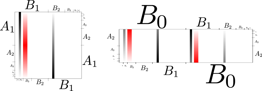
Figure 2. The functions $\bar{w}_{0}$ (in black) and $\bar{w}_{1}$ (in red) on the two presentations of Chamanara’s surface from Figure 1. For $\bar{w}_{0}$, white is 0, black is 1, and grey is in between, whereas for $\bar{w}_{1}$ white is 0, red is 1, and the other shades of red are in between.

Let $\pi:Y_{\mathcal{B}}\rightarrow S_{\mathcal{B}}$ be the map from the (nonsingular) path space to the surface. The paths $p_{m},q_{m}\in E^{Y}_{m-5,m}$ define cylinder sets $[p_{m}],[q_{m}]\subset Y_{\mathcal{B}}$ and the image of these cylinder sets under $\pi$ is denoted by $U_{m},V_{m}\subset S_{\mathcal{B}}$. The functions $w_{m}$ in (2) are in fact the pullback of functions $\bar{w}_{m}$ on $S_{\mathcal{B}}$ which are supported on $U_{m}\cup V_{m}$: $w_{m}=\pi^{*}\bar{w}_{m}$, see Figure 2.

It follows then that $[w_{m}w_{m}^{*}]-2[w_{m+1}w_{m+1}^{*}]$ is in $\ker(j_{*})$. Finally, one can show that under the identification of $\ker(j_{*})$ with $\ker(\iota)$ given in Theorem 10.9, this element corresponds to $I_{m}-I_{m+1}$. This computation is rather long and involves a lot of technical details from the main results of [Put21] that we do not provide. However, given this, it is a fairly simple matter to show that the collection $[w_{m}w_{m}^{*}],m\in\mathbb{Z},$ generates all of $K_{0}(C^{*}(\mathcal{F}_{\mathcal{B}}))$ and has no relations, completing the proof of our claim above that the group is free abelian with a generating set indexed by the integers.

12. Translation surfaces of finite genus

The general goal of this section is to relate our constructions to the well-established study of translation surfaces in the finite genus case. More specifically, we aim to show that all finite genus translation surfaces whose vertical and horizontal foliations are minimal arise via our construction or, to be more precise, to see how standard techniques may be used to produce ordered Bratteli diagrams for finite genus surfaces.

There are several equivalent ways to define a compact translation surface. Here we give two and refer the reader to [Via06, Zor06, FM14] for thorough introductions to flat surfaces.

Let $S$ be a compact Riemann surface of genus $g>1$ and $\alpha$ a 1-form on $S$ which is holomorphic with respect to the complex structure on $S$. The pair $(S,\alpha)$ defines a flat surface and a pair of transverse foliations, the horizontal and vertical foliations, $\mathcal{F}^{\pm}$. These are the foliations defined by the integrable distributions of the real and imaginary parts of $\alpha$:

$$\mathcal{F}^{+}=\langle\ker\Im\alpha\rangle\hskip 72.26999pt\mbox{ and }\hskip 72.26999pt\mathcal{F}^{-}=\langle\ker\Re\alpha\rangle.$$

The unit-time parametrization of these foliations are respectively the horizontal and vertical flows $\phi_{t}^{+}$ and $\phi_{t}^{-}$.

By the Poincaré-Hopf index theorems, since $g>1$, these foliations (and the corresponding flows) are singular; the singular points are the zeros of $\alpha$ and these are called the singularities of $\alpha$, which are denoted by $\Sigma$. The 1-form $\alpha$ gives $S$ a flat metric on $S\setminus\Sigma$ as follows. Let $p\in S\setminus\Sigma$ and $p^{\prime}$ in a neighborhood of $p$. The map $p^{\prime}\mapsto\int_{p}^{p^{\prime}}\alpha\in\mathbb{C}$ defines a chart around $p$ such that the pullback of $dz$ is $\alpha$. This gives $S\setminus\Sigma$ a flat geometry, and the reader can verify that maps which are change of coordinates between these types of charts are of the form $z\mapsto z+c$, justifying the use of the name translation surface. A saddle connection is a geodesic $\gamma\subseteq S$ with respect to the flat metric which starts and ends in $\Sigma$. More specifically, it satisfies the property that $\partial\gamma\subseteq\Sigma$.

The geometry fails to be flat at the singular points in $\Sigma$. At these points the local coordinate is of the form $d\left(\frac{z^{p+1}}{p+1}\right)=dz^{p}$ for some $p\in\mathbb{N}$, called the degree of the singularity. At a point $z\in\Sigma$ of degree $p$, the conical angle around $z$ is $2\pi(p+1)$. If $\Sigma=\{z_{1},\dots,z_{k}\}$, and the degree at $z_{i}$ is $\kappa_{i}$, then by the Gauss-Bonnet theorem we have that $\sum_{i=1}^{k}\kappa_{i}=2g-2$. Since the holomorphic 1-form $\alpha$ determines the geometry of the flat surface $(S,\alpha)$, it defines its area by $\mbox{Area}(S)=\frac{i}{2}\int_{S}\alpha\wedge\bar{\alpha}$.

Another way to define a flat surface is as follows: start with a $2n$-gon $\bar{P}\subseteq\mathbb{C}$ with the property that edges come in parallel pairs of the same length. That is, $\bar{P}$ has edges $\zeta_{1}^{+},\dots,\zeta_{n}^{+},\zeta_{1}^{-},\dots,\zeta_{n}^{-}$, where $\zeta_{i}^{+}$ and $\zeta_{i}^{-}$ are parallel and of the same length. Let $S=\bar{P}/\sim$ be the object obtained by the identifying pairs of edges which are parallel and of the same length: $\zeta_{i}^{+}\sim\zeta_{i}^{-}$. The holomorphic 1-form on $S$ is the unique one which pulls back as $dz$ on $\mathbb{C}$, although it may be singular at points where different edges meet. The points on $S$ where this happens is the singularity set $\Sigma$. The horizontal and vertical foliations on $S$ are now seen as the horizontal and vertical lines in $\bar{P}$. That this definition is equivalent to the one given above is left as an exercise for the reader who has not seen this before.

Translation surfaces come in families: all translation surfaces of genus $g$ are elements of the moduli space $\mathcal{M}_{g}$ of translation surfaces of genus $g$. The space $\mathcal{M}_{g}$ is finite dimensional and it is stratified into strata $\mathcal{H}(\bar{\kappa})$, where $\bar{\kappa}$ describes how many and which types of singularities the surfaces in $\mathcal{H}(\bar{\kappa})$ are allowed to have. The stratum $\mathcal{H}(\bar{\kappa})$ is locally modeled by $H^{1}(S,\Sigma;\mathbb{C})$. By the remarks above, $\mathcal{H}(\kappa_{1},\dots,\kappa_{d})\subseteq\mathcal{M}_{g}$ if and only if $\bar{\kappa}$ satisfies $\sum\kappa_{i}=2g-2$. The Teichmüller flow is the 1-parameter family of homeomorphisms of $\mathcal{M}_{g}$, taking $(S,\alpha)\mapsto(S,\alpha_{t})=g_{t}(S,\alpha)$, where $\Re\alpha_{t}=e^{-t}\Re\alpha$ and $\Im\alpha_{t}=e^{t}\Im\alpha$.

In the rest of this section, we establish a way of defining an ordered, bi-infinite Bratteli diagram $\mathcal{B}(S,\alpha)$ for a typical choice of compact flat surface $(S,\alpha)$.

12.1. Veech’s zippered rectangles

Veech [Vee82] introduced a way of presenting flat surfaces as the union of rectangles which are “zippered” on their sides. Here we review the construction. We will follow the conventions of Viana [Via06].

Let $\mathcal{A}$ be an alphabet of size $d\geq 4$, whose elements are usually written as $\alpha$, and $\pi_{0},\pi_{1}:\mathcal{A}\rightarrow\{1,\dots,d\}$ two bijections. We will consider examples with $\mathcal{A}=\{A,B,C,D\}$. We will use $\alpha$ to denote the inverses of these functions, but instead of writing $\alpha_{\varepsilon}(i)=\pi_{\varepsilon}^{-1}(i)$, for $\varepsilon=0,1,1\leq i\leq d$, we write $\alpha_{i}^{\varepsilon}$. These bijections may be written conveniently as

$$\pi=\left(\begin{array}[]{cccc}\alpha_{1}^{0}&\alpha_{2}^{0}&\cdots&\alpha_{d}^{0}\\ \alpha_{1}^{1}&\alpha_{2}^{1}&\cdots&\alpha_{d}^{1}\end{array}\right),$$

the top and bottom rows being ordered lists of the elements of $\mathcal{A}$. It will always be assumed here that $\pi$ defines an irreducible permutation, in the sense that there is no $k<d$ such that $\pi_{1}\circ\pi_{0}^{-1}\{1,\dots,k\}=\{1,\dots,k\}$.

Figure 3. The flat surface defined by the vectors $\zeta_{i}=(\lambda,\tau)\in\mathbb{R}^{\mathcal{A}}_{+}\times T^{+}_{\pi}$.

We will now define vectors, $(\lambda_{\alpha},\tau_{\alpha})$ in the plane, indexed by $\alpha$ in $\mathcal{A}$. Each $\lambda_{\alpha}$ will be required to be positive while $\tau$ satisfies

(3) $$\sum_{\pi_{0}(\alpha)\leq k}\tau_{\alpha}>0\mbox{ and }\sum_{\pi_{1}(\alpha)\leq k}\tau_{\alpha}<0,$$

for all $k<d$. We let $\mathbb{R}_{+}^{\mathcal{A}}$ to denote positive vectors and $T^{+}_{\pi}$ denote the set of all $\tau$ in $\mathbb{R}^{\mathcal{A}}$ satisfying inequalities (3). Given $\zeta=(\lambda,\tau)$ in$\mathbb{R}^{\mathcal{A}}_{+}\times T^{+}_{\pi}$, let $\Gamma=\Gamma(\pi,\lambda,\tau)\subseteq\mathbb{R}^{2}$ be the curve bounded by the concatenation of the vectors defined by $\zeta$:

$$\zeta_{\alpha_{1}^{0}},\zeta_{\alpha_{2}^{0}},\cdots,\zeta_{\alpha_{d}^{0}},-\zeta_{\alpha_{d}^{1}}^{1},-\zeta_{\alpha_{d-1}^{1}}^{1},\cdots,-\zeta_{\alpha_{1}^{1}}^{1}.$$

The constraints which define $T^{+}_{\pi}$ imply that about half of the vertices of $\Gamma$ are on the upper half plane, and the other rough half on the lower half plane. Assuming $\Gamma$ has no self-intersections, the vector $\zeta$ defines a flat surface by first defining $\zeta_{i}^{+}$ and $\zeta^{-}_{i}$ to be the corresponding edges in the concatenation above in the upper and lower half of the plane, respectively, and then considering the interior of $\Gamma$ and making the identifications $\zeta_{i}^{+}\sim\zeta_{i}^{-}$ on the boundary edges (see Figure 3).

Given the data $(\pi,\lambda,\tau)$ as above, we now define the vector $h$ in $\mathbb{R}^{\mathcal{A}}$ by

$$h_{\alpha}=-\sum_{\pi_{1}(\beta)<\pi_{1}(\alpha)}\tau_{\beta}+\sum_{\pi_{0}(\beta)<\pi_{0}(\alpha)}\tau_{\beta}.$$

This is more concretely expressed as $h=-\Omega_{\pi}(\tau)$, where $\Omega_{\pi}:\mathbb{R}^{\mathcal{A}}\rightarrow\mathbb{R}^{\mathcal{A}}$ is the matrix defined by

$$\Omega_{\alpha\beta}=\left\{\begin{array}[]{ll}+1&\mbox{ if $\pi_{1}(\alpha)>\pi_{1}(\beta)$ and $\pi_{0}(\alpha)<\pi_{0}(\beta)$,}\\ \ -1&\mbox{ if $\pi_{1}(\alpha)<\pi_{1}(\beta)$ and $\pi_{0}(\alpha)>\pi_{0}(\beta)$,}\\ 0&\mbox{ otherwise.}\end{array}\right.$$

Note that, the assumption that $\tau$ is in $T^{+}_{\pi}$ implies that $h_{\alpha}>0$ for all $\alpha$ in $\mathcal{A}$. We define the image of the positive cone $T^{+}_{\pi}$ under $-\Omega_{\pi}$ by $H^{+}_{\pi}=-\Omega_{\pi}(T^{+}_{\pi})$.

We now define rectangles $R_{\alpha}^{\varepsilon}$ of width $\lambda_{\alpha}$ and height $h_{\alpha}$ by

(4) $$\begin{split}R_{\alpha}^{0}&=\left(\sum_{\pi_{0}(\beta)<\pi_{0}(\alpha)}\lambda_{\beta},\sum_{\pi_{0}(\beta)\leq\pi_{0}(\alpha)}\lambda_{\beta}\right)\times[0,h_{\alpha}]\\ R_{\alpha}^{1}&=\left(\sum_{\pi_{1}(\beta)<\pi_{1}(\alpha)}\lambda_{\beta},\sum_{\pi_{1}(\beta)\leq\pi_{1}(\alpha)}\lambda_{\beta}\right)\times[-h_{\alpha},0].\end{split}$$

along with the “zippers”

$$\begin{split}Z_{\alpha}^{0}&=\left\{\sum_{\pi_{0}(\beta)\leq\pi_{0}(\alpha)}\lambda_{\beta}\right\}\times\left[0,\sum_{\pi_{0}(\beta)\leq\pi_{0}(\alpha)}\tau_{\beta}\right]\\ Z_{\alpha}^{1}&=\left\{\sum_{\pi_{1}(\beta)\leq\pi_{1}(\alpha)}\lambda_{\beta}\right\}\times\left[\sum_{\pi_{1}(\beta)\leq\pi_{1}(\alpha)}\tau_{\beta},0\right]\\ \end{split}$$

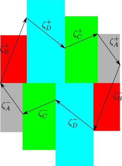
Figure 4. The zippered rectangles for the surface in Figure 3.

which are vertical segments ending at the points of concatenation of the curve $\Gamma$. As such, the flat surface $S(\pi,\lambda,\tau)$ can be presented as the quotient of the closure of the union of the rectangles $\{R_{\alpha}^{0}\}_{\alpha\in\mathbb{R}^{\mathcal{A}}}$ and zippers under a relation defined on the edges of the rectangles. The genus $g$ of this surface satisfies $2g=\mathrm{dim}\,\Omega_{\pi}(\mathbb{R}^{\mathcal{A}})$. The area of the surface is $\mathrm{Area}(S(\pi,\lambda,\tau))=\lambda\cdot h$. Moreover, the horizontal and vertical foliations are the obvious choices. See Figure 4.

12.2. Rauzy-Veech Induction

Given a triple $(\pi,\lambda,\tau)$, where $\pi=\{\pi_{0},\pi_{1}\}$ is an irreducible permutation, $\lambda$ in $\mathbb{R}^{\mathcal{A}}_{+}$ and $\tau$ in $T^{+}_{\pi}$, we will define an operation which produces a new triple $(\pi^{\prime},\lambda^{\prime},\tau^{\prime})$ with the same properties. This procedure is known as Rauzy-Veech induction, or RV induction.

First, let us describe what this procedure is meant to do geometrically, and then we will give the details as to how it is done. Recall that from the triple $(\pi,\lambda,\tau)$ the flat surface it defines can be presented in zippered recangles form. The map $\mathcal{R}(\pi,\lambda,\tau)=(\pi^{\prime},\lambda^{\prime},\tau^{\prime})$ gives new data from which the same surface can be presented in zippered rectangle form, except that the base one of the rectangles will be shorter and the height of one of the rectangles will be longer. This is done by cutting one of the rectangles $R_{\alpha}^{\varepsilon}$ into two and stacking one of the subrectangles above or below another one of the rectangles. The choices of the rectangles picked for this operation are determined by $(\pi,\lambda)$.

Remark 12.1.

It will be important to keep in mind one of the benefits of using Rauzy-Veech induction: it allows us to understand the behavior of the leaf of the vertical foliation on $S(\pi,\lambda,\tau)$ which emanates from the point on this surface coming from the origin in $\mathbb{R}^{2}$. An analogous procedure for the horizontal foliation will be described in §12.3.

First, we define $\pi^{\prime}$ and $\lambda^{\prime}$. Let $\alpha(\varepsilon)=\pi^{-1}_{\varepsilon}(d)=\alpha_{d}^{\varepsilon}$. That is, $\alpha(0)$ and $\alpha(1)$ are the last entries in the top and bottom rows of $\pi$.

Definition 12.2.

We say that $(\pi,\lambda)$ has

$$\mbox{{type 0} if $\lambda_{\alpha(0)}>\lambda_{\alpha(1)}$\hskip 50.58878pt or\hskip 50.58878pt {type 1} if $\lambda_{\alpha(0)}<\lambda_{\alpha(1)}$}.$$

If $(\pi,\lambda)$ is of type $\varepsilon\in\{0,1\}$ then the winner is the symbol $\alpha(\varepsilon)$ and the loser is $\alpha(1-\varepsilon)$.

This makes sense as long as $\lambda_{\alpha(0)}\neq\lambda_{\alpha(1)}$, so we will make the following assumption, to which we will return later.

Hypothesis 12.3.

The pair $(\pi,\lambda)$ satisfies $\lambda_{\alpha(0)}\neq\lambda_{\alpha(1)}$.

If $(\pi,\lambda)$ has type 0, then $\pi^{\prime}$ is defined by

(5) $$\pi^{\prime}=\left(\begin{array}[]{cccccccc}\alpha_{1}^{0}&\cdots&\alpha_{k-1}^{0}&\alpha_{k}^{0}&\alpha_{k+1}^{0}&\cdots&\cdots&\alpha(0)\\ \alpha_{1}^{1}&\cdots&\alpha_{k-1}^{1}&\alpha(0)&\alpha(1)&\alpha^{1}_{k+1}&\cdots&\alpha^{1}_{d-1}\end{array}\right),$$

that is,

$$\alpha_{i}^{0^{\prime}}=\alpha_{i}^{0}\hskip 28.90755pt\mbox{ and }\hskip 28.90755pt\alpha^{1^{\prime}}_{i}=\left\{\begin{array}[]{ll}\alpha_{i}^{1}&\mbox{ if $i\leq\pi_{1}(\alpha(0))$}\\ \alpha(1)&\mbox{ if $i=\pi_{1}(\alpha(0))+1$}\\ \alpha_{i-1}^{1}&\mbox{ if $i>\pi_{1}(\alpha(0))+1$}\end{array}\right..$$

The vector $\lambda^{\prime}$ is now defined by

(6) $$\lambda_{\alpha}^{\prime}=\lambda_{\alpha}\mbox{ if $\alpha\neq\alpha(0)$\;\;\; and \;\;\; $\lambda_{\alpha(0)}^{\prime}=\lambda_{\alpha(0)}-\lambda_{\alpha(1)}$},$$

whereas $\tau^{\prime}$ is defined by

(7) $$\tau_{\alpha}^{\prime}=\tau_{\alpha}\mbox{ if $\alpha\neq\alpha(0)$\;\;\;and \;\;\; $\tau_{\alpha(0)}^{\prime}=\tau_{\alpha(0)}-\tau_{\alpha(1)}$}.$$

If $(\pi,\lambda)$ has type 1, then $\pi^{\prime}$ is defined by

(8) $$\pi^{\prime}=\left(\begin{array}[]{cccccccc}\alpha_{1}^{0}&\cdots&\alpha_{k-1}^{0}&\alpha(1)&\alpha(0)&\alpha^{0}_{k+1}&\cdots&\alpha^{0}_{d-1}\\ \alpha_{1}^{1}&\cdots&\alpha_{k-1}^{1}&\alpha_{k}^{1}&\alpha_{k+1}^{1}&\cdots&\cdots&\alpha(1)\end{array}\right),$$

that is,

$$\alpha_{i}^{1^{\prime}}=\alpha_{i}^{1}\hskip 28.90755pt\mbox{ and }\hskip 28.90755pt\alpha^{0^{\prime}}_{i}=\left\{\begin{array}[]{ll}\alpha_{i}^{0}&\mbox{ if $i\leq\pi_{0}(\alpha(1))$}\\ \alpha(0)&\mbox{ if $i=\pi_{0}(\alpha(1))+1$}\\ \alpha_{i-1}^{1}&\mbox{ if $i>\pi_{0}(\alpha(1))+1$}\end{array}\right..$$

The vector $\lambda^{\prime}$ is now defined by

(9) $$\lambda_{\alpha}^{\prime}=\lambda_{\alpha}\mbox{ if $\alpha\neq\alpha(1)$\;\;\; and \;\;\; $\lambda_{\alpha(1)}^{\prime}=\lambda_{\alpha(1)}-\lambda_{\alpha(0)}$},$$

whereas $\tau^{\prime}$ is defined by

(10) $$\tau_{\alpha}^{\prime}=\tau_{\alpha}\mbox{ if $\alpha\neq\alpha(1)$\;\;\;and \;\;\; $\tau_{\alpha(1)}^{\prime}=\tau_{\alpha(1)}-\tau_{\alpha(0)}$}.$$

Let $\Theta=\Theta_{\pi,\lambda}:\mathbb{R}^{\mathcal{A}}\rightarrow\mathbb{R}^{\mathcal{A}}$ be the matrix defined, when $(\pi,\lambda)$ has type 0,as

$$\Theta_{\alpha\gamma}=\left\{\begin{array}[]{ll}1&\mbox{ if }\alpha=\gamma\\ 1&\mbox{ if $\alpha=\alpha(1)$ and $\gamma=\alpha(0)$}\\ 0&\mbox{ otherwise}\end{array}\right.$$

whose inverse is

$$\Theta_{\alpha\gamma}^{-1}=\left\{\begin{array}[]{ll}1&\mbox{ if }\alpha=\gamma\\ -1&\mbox{ if $\alpha=\alpha(1)$ and $\gamma=\alpha(0)$}\\ 0&\mbox{ otherwise.}\end{array}\right.$$

When $(\pi,\lambda)$ has type 1,

$$\Theta_{\alpha\gamma}=\left\{\begin{array}[]{ll}1&\mbox{ if }\alpha=\gamma\\ 1&\mbox{ if $\alpha=\alpha(0)$ and $\gamma=\alpha(1)$}\\ 0&\mbox{ otherwise}\end{array}\right.$$

whose inverse is

$$\Theta_{\alpha\gamma}^{-1}=\left\{\begin{array}[]{ll}1&\mbox{ if }\alpha=\gamma\\ -1&\mbox{ if $\alpha=\alpha(0)$ and $\gamma=\alpha(1)$}\\ 0&\mbox{ otherwise.}\end{array}\right.$$

This matrix satisfies [Via06, Lemma 10.2] the relation

(11) $$\Theta\Omega_{\pi}\Theta^{*}=\Omega_{\pi^{\prime}}.$$

As such, the relations between $\lambda$ and $\lambda^{\prime}$ and between $\tau$ and $\tau^{\prime}$, are expressed by

$$\lambda^{\prime}=\Theta^{-1*}\lambda\hskip 14.45377pt\mbox{ or }\hskip 14.45377pt\lambda=\Theta^{*}\lambda^{\prime},\hskip 21.68121pt\mbox{ and }\hskip 21.68121pt\tau^{\prime}=\Theta^{-1*}\tau,$$

and so Rauzy-Veech induction is the map

$$\mathcal{R}:(\pi,\lambda,\tau)\mapsto(\pi^{\prime},\Theta^{-1*}\lambda,\Theta^{-1*}\tau).$$

In terms of zippered rectangles, RV induction has an explicit expression in terms of the height vector $h=-\Omega_{\pi}(\tau)$ in $H^{+}_{\pi}$. Indeed, we have that $\Theta\Omega_{\pi}=\Omega_{\pi^{\prime}}\Theta^{-1*}$ and so denoting $h^{\prime}=-\Omega_{\pi^{\prime}}(\tau^{\prime})$ the corresponding height vector for $\tau^{\prime}$, we have that $h^{\prime}=\Theta h$. It is straight forward to verify that if $\tau$ in $T^{+}_{\pi}$ then $\tau^{\prime}$ in $T^{+}_{\pi^{\prime}}$. As such, the surface $S(\pi^{\prime},\lambda^{\prime},\tau^{\prime})$ has area

$$\begin{split}\mathrm{Area}(S(\pi^{\prime},\lambda^{\prime},\tau^{\prime}))&=\lambda^{\prime}\cdot(-\Omega_{\pi^{\prime}}(\tau^{\prime}))=-\Theta^{-1*}\lambda\cdot\Theta\Omega_{\pi}\Theta^{*}(\tau^{\prime})=-\Theta^{-1*}\lambda\cdot\Theta\Omega_{\pi}(\tau)\\ &=\Theta^{-1*}\lambda\cdot\Theta h=\lambda\cdot h=\mathrm{Area}(S(\pi,\lambda,\tau)).\end{split}$$

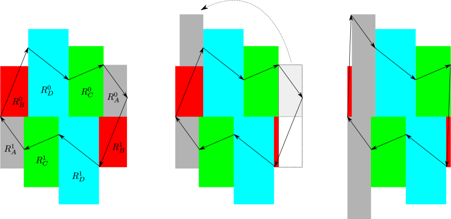
Figure 5. Geometric illustration of Rauzy-Veech induction. Since $\lambda_{\alpha(1)}>\lambda_{\alpha(0)}$, this corresponds to type 1.

Geometrically, Rauzy-Veech induction makes a vertical cut through the widest rectangle at the end, takes the right subrectangle, and stacks it above or below the rectangle according to the rules described above. Figure 5 illustrates an example of what Rauzy-Veech induction does to the zippered rectangles and the surface it represents from Figure 4.

Note that in the definition of RV induction, whenever it was defined (Hypothesis 12.3), we may have that $\pi^{\prime}\neq\pi$. Thus we can consider all possible permutations that can be obtained from $\pi$ under RV induction.

Definition 12.4.

The Rauzy graph $\mathcal{G}_{d}$ of permutations on $d$ elements is the directed graph which has as vertices equivalence classes of permutations $\pi=\{\pi_{0},\pi_{1}\}$, where $\pi\sim\pi^{\prime}$ whenever $\pi_{1}\circ\pi_{0}^{-1}=\pi_{1}^{\prime}\circ\pi_{0}^{-1^{\prime}}$, and there is an edge from $[\pi]$ to $[\pi^{\prime}]$ if there are representatives $\pi$, $\pi^{\prime}$ and vector $\lambda$ in $\mathbb{R}^{\mathcal{A}}_{+}$ such that $\pi^{\prime}$ is the permutation obtained from $(\pi,\lambda)$ through Rauzy-Veech induction. A Rauzy class is by connected components of the Rauzy graph.

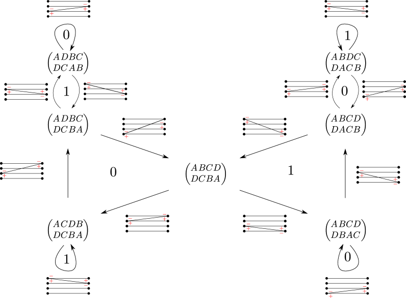
Figure 9. The Rauzy graph for surfaces in the hyperelliptic component of $\mathcal{H}(2)$. The arrows represent a step of RH induction depending on the $\tau$-type in $\{0,1\}$. Next to every arrow is the edge set associated to the Bratteli diagram: if $(\pi,\lambda,\tau)$ is RH-complete, then it defines an infinite walk on this graph, and the edge set $E_{n}$ is defined by the edge set corresponding to the arrow above in the $n^{th}$ step. If $(\pi,\lambda,\tau)$ satisfies the Keane condition, then it defines an infinite backwards walk on this graph and the edge sets of the Bratteli diagram $\mathcal{B}_{\pi,\lambda,\tau}$ are defined accordingly.

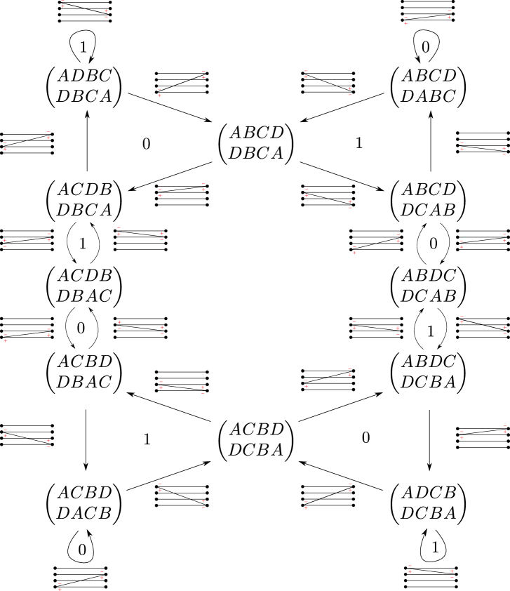
Figure 10. Rauzy graph for surfaces in the non-hyperelliptic component of $\mathcal{H}(2)$ along with corresponding edge sets for the Bratteli diagrams.

There are two outgoing edges from each class $[\pi]$, one for each type, as well as two incoming edges. See Figures 9 and 10 for examples in genus 2.

Let $(\pi,\lambda,\tau)$ in $\mathcal{C}\times\mathbb{R}^{\mathcal{A}}\times T^{+}_{\pi}$ satisfying Hypothesis 12.3. Then the map $\mathcal{R}$ is well defined, and we obtain $(\pi^{\prime},\lambda^{\prime},\tau^{\prime})=\mathcal{R}(\pi,\lambda,\tau)$ in $\mathcal{C}\times\mathbb{R}^{\mathcal{A}}\times T^{+}_{\pi}$. We would like to once again apply $\mathcal{R}$ to this new data, but we do not know a-priori whether $(\pi^{\prime},\lambda^{\prime},\tau^{\prime})$ satisfies Hypothesis 12.3.

To establish conditions for which all iterates of RV induction are defined, we first need to define the interval exchange transformation (IET) defined by $(\pi,\lambda)$. For $\alpha$ in $\mathcal{A}$, let

$$I_{\alpha}=\left[\sum_{\pi_{0}(\gamma)<\pi_{0}(\alpha)}\lambda_{\gamma},\sum_{\pi_{0}(\gamma)\leq\pi_{0}(\alpha)}\lambda_{\gamma}\right)$$

and with $|I|=\|\lambda\|_{1}$, the IET $f:[0,|I|)\rightarrow[0,|I|)$ defined by $(\pi,\lambda)$ is

$$f(x)=x+\Omega_{\pi}(\lambda)_{\alpha}\mbox{ for $x\in I_{\alpha}$}.$$

The reader is encouraged now to verify that the zippered rectangle surfaces in §12.1 are suspensions over the IET $f$ with roof functions given by the height vector $h$. Denote by $\partial I_{\alpha}$ the left endpoint of the interval $I_{\alpha}$.

Definition 12.5.

A pair $(\pi,\lambda)$ satisfies the Keane condition if $f^{m}(\partial I_{\alpha})\neq\partial I_{\gamma}$ for all $m$ in $\mathbb{N}$ and $\alpha,\gamma\in\mathcal{A}$ with $\pi_{0}(\gamma)\neq 1$.

Remark 12.6.

1. This condition guarantees that the orbits of the left endpoints of the intervals are as disjoint as possible. This surely guarantees Hypothesis 12.3. Below we will see that this characterizes the good data for which RV induction is defined for all iterates.

2. It is known that the Keane condition implies the minimality of the interval exchange transformation $f$, that is, that every orbit is dense. This in turn implies that the vertical foliation on $S(\pi,\lambda,\tau)$ has no closed leaves and every leaf is dense in the surface.

Theorem 12.7.

The following are equivalent:

1. $(\pi,\lambda)$ satisfies the Keane condition.

2. All iterates $\mathcal{R}^{n}(\pi,\lambda)$ of Rauzy-Veech induction are defined for $n>0$.

3. For each $\alpha$ in $\mathcal{A}$, there is a subsequence $n_{i}^{\alpha}\rightarrow\infty$ such that $\alpha$ is the winner for $\mathcal{R}^{n_{i}^{\alpha}}(\pi,\lambda)$ for every $i$.

4. For each $\alpha$ in $\mathcal{A}$, there is a subsequence $n_{i}^{\alpha}\rightarrow\infty$ such that $\alpha$ is the loser for $\mathcal{R}^{n_{i}^{\alpha}}(\pi,\lambda)$ for every $i$.

Moreover, these equivalent conditions are satisfied on a full measure subset of the space of parameters.

For a proof, see [Via06, §5]. Thus, it is better to replace Hypothesis 12.3 with the Keane condition.

12.3. RH Induction

The previous section reviewed a procedure which, starting with some data $(\pi,\lambda,\tau)$ and depending only on $\pi$ and $\lambda$, produced a new triple $\mathcal{R}(\pi^{\prime},\lambda^{\prime},\tau^{\prime})$. Moreover, there is a precise condition that characterizes all data for which all iterates of this procedure are defined. Denoting by $(\pi^{(n)},\lambda^{(n)},\tau^{(n)})=\mathcal{R}^{n}(\pi,\lambda,\tau)$, the surfaces $S(\pi^{(n)},\lambda^{(n)},\tau^{(n)})$ are different presentations of $S(\pi,\lambda,\tau)$ which allow us to keep track of longer and longer segments of the vertical leaf emanating from the origin.

In this section, we define a different procedure, $\mathcal{P}:(\pi,\lambda,\tau)\mapsto(\pi^{\prime},\lambda^{\prime},\tau^{\prime})$, with the aim of doing the same for the trajectory of the horizontal foliation emanating from the origin, that is, we will get presentations $S(\pi^{(n)},\lambda^{(n)},\tau^{(n)})$ of $S(\pi,\lambda,\tau)$ through $(\pi^{(n)},\lambda^{(n)},\tau^{(n)})=\mathcal{P}^{n}(\pi,\lambda,\tau)$ which will allow us to capture longer and longer segments of the horizontal leaf emanating from the origin. We will then relate this procedure to RV induction. This exposition is our own, but the recent work [Ber21] captures most of the aspects presented here.

Let us first describe and illustrate how this procedure is meant to work and then we will give the details. Let $(\pi,\lambda,\tau)$ in $\mathcal{C}\times\mathbb{R}^{\mathcal{A}}_{+}\times T^{+}_{\pi}$ and consider the zippered rectangles presentation of it in (4). Our goal is to extend $[0,|I|)$ to $[0,|I^{\prime}|)$, where $|I^{\prime}|=\|\lambda^{\prime}\|_{1}$. Given $\pi=(\pi_{0},\pi_{1})$, define

(12) $$\beta(\varepsilon)=\pi_{\varepsilon}^{-1}(\pi_{\varepsilon}(\alpha(1-\varepsilon))+1),$$

for $\varepsilon=\{0,1\}$. In words, $\beta(\varepsilon)$ is the symbol immediately to the right of $\alpha_{d}^{1-\varepsilon}$ on $\pi_{\varepsilon}$.

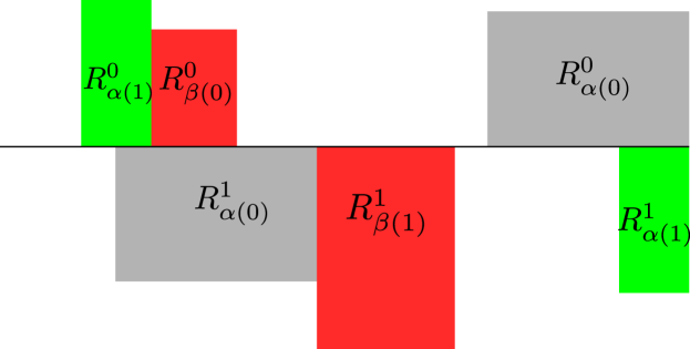
Figure 6. The case $h_{\alpha(1)}>h_{\beta(0)}$ and $h_{\alpha(0)}<h_{\beta(1)}$.

Suppose for the moment that $h_{\alpha(1)}>h_{\beta(0)}$ and $h_{\alpha(0)}<h_{\beta(1)}$ (see Figure 6). In order to extend the horizontal leaf starting at the origin, it must come out of the bottom edge of the rectangle $R^{1}_{\alpha(0)}$ cut through $R^{1}_{\beta(1)}$, subdividing it into two subrectangles. The top rectangle will be absorbed into a larger rectangle $R^{1}_{\alpha^{\prime}(0)}=R^{1}_{\alpha(0)}$, while the bottom rectangle will be moved to the right and become $R^{1}_{\alpha^{\prime}(1)}$. Thus, we extend $[0,|I|)$ by $\lambda_{\beta(1)}$ and rearrange the rectangles as in Figure 7.

If $h_{\alpha(1)}<h_{\beta(0)}$ and $h_{\alpha(0)}>h_{\beta(1)}$ then an analogous procedure is defined by cutting through the rectangle $R^{0}_{\beta(0)}$ and moving the top rectangle to the right-most place on the top set of rectangles.

It may be unclear how to proceed if $h_{\alpha(1)}<h_{\beta(0)}$ and $h_{\alpha(0)}<h_{\beta(1)}$, as in Figure 4. What really determines which rectangle to cut has to do with the $\tau\in T^{+}_{\pi}$ which defines $h=-\Omega_{\pi}(\tau)$. Indeed, in the case $h_{\alpha(1)}>h_{\beta(0)}$ and $h_{\alpha(0)}<h_{\beta(1)}$ as in Figure 6 the zipper between $R^{0}_{\alpha(1)}$ and $R^{0}_{\beta(0)}$ is somewhere in the interior of the right edge of $R^{0}_{\alpha(1)}$, meaning that it is on the right edge of $R^{1}_{\alpha(1)}$, meaning that $\sum_{\alpha}\tau_{\alpha}<0$. Likewise, $h_{\alpha(1)}<h_{\beta(0)}$ and $h_{\alpha(0)}>h_{\beta(1)}$ imply that $\sum_{\alpha}\tau_{\alpha}>0$.

Let us remark that the case $h_{\alpha(1)}>h_{\beta(0)}$ and $h_{\alpha(0)}>h_{\beta(1)}$ is impossible. Indeed, consider the zipper between $R^{0}_{\alpha(1)}$ and $R^{0}_{\beta(0)}$. There is a singularity of the flat surface somewhere between these two rectangles. But this singularity is to the right of $R^{0}_{\alpha(1)}$, which means that there is a singularity on the right edge of $R^{1}_{\alpha(1)}$, which has to have height $\sum_{\alpha}\tau_{\alpha}<0$. The same argument for the rectangles $R^{1}_{\alpha(0)}$ and $R^{1}_{\beta(1)}$ implies that $\sum_{\alpha}\tau_{\alpha}>0$. Since $\tau\in T^{+}_{\pi}$, it satisfies one of the two conditions of (3), so it is impossible to have $h_{\alpha(1)}>h_{\beta(0)}$ and $h_{\alpha(0)}>h_{\beta(1)}$.

Hypothesis 12.8.

The pair $(\pi,\tau)$ with $\tau$ in $T^{+}_{\pi}$ satisfies $\sum_{\alpha}\tau_{\alpha}\neq 0$.

Motivated by this discussion and following the terminology [Via06, §12], we have the following definition.

Definition 12.9.

If the pair $(\pi,\tau)$ satisfies Hypothesis 12.8, it will be called

$$\mbox{{Type $0$} if $\displaystyle\sum_{\alpha}\tau_{\alpha}>0$\ \hskip 50.58878pt or \hskip 50.58878pt {Type $1$} if $\displaystyle\sum_{\alpha}\tau_{\alpha}<0$}.$$

If $(\pi,\tau)$ is of type $\varepsilon\in\{0,1\}$ then the $\tau$-winner is the symbol $\alpha(1-\varepsilon)$.

Thus if $(\pi,\tau)$ is type $0$, then the rectangle $R^{0}_{\beta(0)}$ will be subdivided into two rectangles, the bottom part will be absorbed into $R^{0}_{\alpha(1)}$ while the top part will be moved to the right to become $R_{d}^{0^{\prime}}$. If $(\pi,\tau)$ is type $1$, the rectangle $R^{1}_{\beta(1)}$ will be subdivided into two rectangles, the top part will be absorbed into $R^{1}_{\alpha(0)}$ while the top part will be moved to the right to become $R_{d}^{1^{\prime}}$, as depicted in Figure 7.

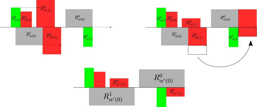
Figure 7. Starting from Figure 6, the procedure producing a new zippered rectangles presentation implies that $\alpha^{\prime}(0)=\alpha(0)$ and $\alpha^{\prime}(1)=\beta(1)$. Compare with Figure 5.

These operations are formally defined as follows. Let $\tau$ in $T^{+}_{\pi}$ be of type $0$. Starting with $(\pi,\lambda,\tau)$ and based on the description in the previous paragraph, the new data $(\pi^{\prime},\lambda^{\prime},h^{\prime})=\mathcal{P}(\pi,\lambda,h)=\mathcal{P}(\pi,\lambda,-\Omega_{\pi}(\tau))$ is defined, first, by letting

(13) $$\pi^{\prime}=\left(\begin{array}[]{cccccccc}\alpha_{1}^{0}&\cdots&\alpha_{k-1}^{0}&\alpha(1)&\alpha^{0}_{k+2}&\cdots&\alpha(0)&\beta(0)\\ \alpha_{1}^{1}&\cdots&\alpha_{k-1}^{1}&\alpha_{k}^{1}&\alpha_{k+1}^{1}&\cdots&\cdots&\alpha(1)\end{array}\right),$$

that is,

$$(\alpha^{{}^{\prime}})^{1}_{i}=\alpha_{i}^{1}\hskip 28.90755pt\mbox{ and }\hskip 28.90755pt(\alpha^{{}^{\prime}})^{0}_{i}=\left\{\begin{array}[]{ll}\alpha_{i}^{0}&\mbox{ if $i\leq\pi_{0}(\alpha(1))$}\\ \alpha^{0}_{i+1}&\mbox{ if $\pi_{0}(\alpha(1))<i<d$}\\ \beta(0)&\mbox{ if $i=d$}\end{array}\right..$$

The vector $\lambda^{\prime}$ is now defined by

(14) $$\lambda_{\alpha}^{\prime}=\lambda_{\alpha}\mbox{ if $\alpha\neq\alpha(1)$\;\;\; and \;\;\; $\lambda_{\alpha(1)}^{\prime}=\lambda_{\alpha(1)}+\lambda_{\beta(0)}$},$$

whereas $h^{\prime}$ is defined by

(15) $$h_{\alpha}^{\prime}=h_{\alpha}\mbox{ if $\alpha\neq\beta(0)$\;\;\;and \;\;\; $h_{\beta(0)}^{\prime}=h_{\beta(0)}-h_{\alpha(1)}$}.$$

The definition of $\tau^{\prime}$ will follow from Proposition 12.9.

Let $\tau$ in $T^{+}_{\pi}$ be of type $1$. Starting from $(\pi,\lambda,\tau)$ we now define $(\pi^{\prime},\lambda^{\prime},h^{\prime})$ by

(16) $$\pi^{\prime}=\left(\begin{array}[]{cccccccc}\alpha_{1}^{0}&\cdots&\alpha_{k-1}^{0}&\alpha_{k}^{0}&\alpha_{k+1}^{0}&\cdots&\cdots&\alpha(0)\\ \alpha_{1}^{1}&\cdots&\alpha_{k-1}^{1}&\alpha(0)&\alpha^{1}_{k+2}&\cdots&\alpha(1)&\beta(1)\end{array}\right),$$

that is,

$$\alpha_{i}^{0^{\prime}}=\alpha_{i}^{0}\hskip 28.90755pt\mbox{ and }\hskip 28.90755pt\alpha^{1^{\prime}}_{i}=\left\{\begin{array}[]{ll}\alpha_{i}^{1}&\mbox{ if $i\leq\pi_{1}(\alpha(0))$}\\ \alpha^{1}_{i+1}&\mbox{ if $\pi_{1}(\alpha(0))<i<d$}\\ \beta(1)&\mbox{ if $i=d$}\end{array}\right..$$

The vector $\lambda^{\prime}$ is now defined by

(17) $$\lambda_{\alpha}^{\prime}=\lambda_{\alpha}\mbox{ if $\alpha\neq\alpha(0)$\;\;\; and \;\;\; $\lambda_{\alpha(0)}^{\prime}=\lambda_{\alpha(0)}+\lambda_{\beta(1)}$},$$

whereas $h^{\prime}$ is defined by

(18) $$h_{\alpha}^{\prime}=h_{\alpha}\mbox{ if $\alpha\neq\beta(1)$\;\;\;and \;\;\; $h_{\beta(1)}^{\prime}=h_{\beta(1)}-h_{\alpha(0)}$}.$$

The definition of $\tau^{\prime}$ will follow from Proposition 12.9.

Let $\Psi=\Psi_{\pi,h}:\mathbb{R}^{\mathcal{A}}\rightarrow\mathbb{R}^{\mathcal{A}}$ be the matrix defined, when $(\pi,h)$ has type $0$, as

(19) $$\Psi_{\alpha\gamma}=\left\{\begin{array}[]{ll}1&\mbox{ if }\alpha=\gamma\\ 1&\mbox{ if $\alpha=\alpha(1)$ and $\gamma=\beta(0)$}\\ 0&\mbox{ otherwise}\end{array}\right.$$

whose inverse is

$$\Psi_{\alpha\gamma}^{-1}=\left\{\begin{array}[]{ll}1&\mbox{ if }\alpha=\gamma\\ -1&\mbox{ if $\alpha=\alpha(1)$ and $\gamma=\beta(0)$}\\ 0&\mbox{ otherwise.}\end{array}\right.$$

When $(\pi,h)$ has type $1$, as

(20) $$\Psi_{\alpha\gamma}=\left\{\begin{array}[]{ll}1&\mbox{ if }\alpha=\gamma\\ 1&\mbox{ if $\alpha=\alpha(0)$ and $\gamma=\beta(1)$}\\ 0&\mbox{ otherwise}\end{array}\right.$$

whose inverse is

$$\Psi_{\alpha\gamma}^{-1}=\left\{\begin{array}[]{ll}1&\mbox{ if }\alpha=\gamma\\ -1&\mbox{ if $\alpha=\alpha(0)$ and $\gamma=\beta(1)$}\\ 0&\mbox{ otherwise.}\end{array}\right.$$

Thus, the map $\mathcal{P}$ acts on data as $\mathcal{P}:(\pi,\lambda,h)\mapsto(\pi^{\prime},\Psi\lambda,\Psi^{-1*}h)$.

Here we want to pick out a condition, analogous to the Keane condition in Theorem 12.7, which characterizes the data for which $\mathcal{P}^{n}(\pi,\lambda,t)$ is defined for all $n>0$. First observe that if we restrict ourselves to all $h$ with rationally independent entries, that is, to $h\in H^{+}_{\pi}$ so that

(21) $$\sum_{\alpha}n_{\alpha}h_{\alpha}\neq 0\mbox{ for all }n\in\mathbb{Z}^{\mathcal{A}},$$

then $\mathcal{P}^{n}(\pi,\lambda,h)$ is defined for all $n>0$. Moreover, the collection of all such vectors has full measure in $H^{+}_{\pi}$.

Definition 12.10.

The triple $(\pi,\lambda,\tau)$ is RH-complete if for every $\alpha$ in $\mathcal{A}$ there is a subsequence $n_{i}^{\alpha}\rightarrow\infty$ such that $\alpha$ is the $\tau$-winner of $\mathcal{P}^{n_{i}^{\alpha}}(\pi,\lambda,\tau)$ for all $i$.

There is an analogous way to characterize when $\mathcal{P}^{n}$ is defined for all $n>0$ recently proved by Berk (see [Ber21]). Compare the following with Theorem 12.7.

Theorem 12.11 ([Ber21]).

The following are equivalent:

1. All iterates $\mathcal{P}^{n}(\pi,\lambda,\tau)$ of RH-induction are defined.

2. $(\pi,\lambda,\tau)$ is RH-complete.

3. The horizontal leaf emanating from the singularity associated to the origin has infinite length.

12.4. Relations between RV and RH inductions

Here, we prove that RH induction is the inverse of RV induction.

Proposition 12.12.

Let $(\pi,\lambda,h)=(\pi,\lambda,-\Omega_{\pi}(\tau))$ with $\tau$ in $T^{+}_{\pi}$. If $\lambda$ in $\mathbb{R}^{\mathcal{A}}_{+}$ satisfies Hypothesis 12.3, then $\mathcal{P}\circ\mathcal{R}=\mathrm{Id}$. If $\tau$ in $T^{+}_{\pi}$ satisfies Hypothesis 12.8, then $\mathcal{R}\circ\mathcal{P}=\mathrm{Id}$.

Proof.

Let $(\pi^{\prime},\lambda^{\prime},h^{\prime})=\mathcal{P}(\pi,\lambda,h)$. Now suppose $\tau$ in $T^{+}_{\pi}$ is of type $0$. Then by (14):

$$\lambda^{\prime}_{\alpha^{\prime}(0)}=\lambda_{\beta(0)}<\lambda_{\beta(0)}+\lambda_{\alpha(1)}=\lambda^{\prime}_{\alpha^{\prime}(1)},$$

which means that $(\pi^{\prime},\lambda^{\prime})$ is of type 1. Comparing (9) and (14), we get that $\mathcal{R}(\lambda^{\prime})_{\alpha}=\lambda^{\prime}_{\alpha}=\lambda_{\alpha}$ whenever $\alpha\neq\alpha^{\prime}(1)=\alpha(1)$ and

$$\mathcal{R}(\lambda^{\prime})_{\alpha^{\prime}(1)}=\lambda^{\prime}_{\alpha^{\prime}(1)}-\lambda^{\prime}_{\alpha^{\prime}(0)}=(\lambda_{\alpha(1)}+\lambda_{\beta(0)})-\lambda_{\beta(0)}=\lambda_{\alpha(1)}.$$

Finally, comparing (8) and (13), we get that $\mathcal{R}\circ\mathcal{P}(\pi,\lambda)=(\pi,\Theta^{-1*}\Psi\lambda)=(\pi,\lambda)$, so $\Psi=\Theta^{*}$. If $\alpha^{\prime}(\varepsilon)$ are the last symbols of the permutation $\pi^{\prime}_{\varepsilon}$, then $\alpha^{\prime}(0)=\beta(0)$. So $\mathcal{R}(h^{\prime})_{\alpha}=h_{\alpha}$ if $\alpha\neq\alpha^{\prime}(0)=\beta(0)$, and

$$\mathcal{R}(h^{\prime})_{\alpha^{\prime}(0)}=h^{\prime}_{\alpha^{\prime}(0)}+h^{\prime}_{\alpha^{\prime}(1)}=h^{\prime}_{\beta(0)}+h^{\prime}_{\alpha(1)}=(h_{\beta(0)}-h_{\alpha(1)})+h_{\alpha(1)}=h_{\beta(0)}=h_{\alpha^{\prime}(0)},$$

so $\mathcal{R}\circ\mathcal{P}(\pi,\lambda,h)=(\pi,\Theta^{-1*}\Psi\lambda,\Theta\Psi^{-1*}h)=(\pi,\lambda,h)$. So $\mathcal{R}\circ\mathcal{P}(\pi,\lambda,h)=(\pi,\lambda,h)$.

Suppose now $\tau$ in $T^{+}_{\pi}$ is of type $1$. Then by (17):

$$\lambda^{\prime}_{\alpha^{\prime}(1)}=\lambda_{\beta(1)}<\lambda_{\beta(1)}+\lambda_{\alpha(0)}=\lambda^{\prime}_{\alpha^{\prime}(0)},$$

which means that $(\pi^{\prime},\lambda^{\prime})$ is of type 0. Comparing (6) and (17), we get that $\mathcal{R}(\lambda^{\prime})_{\alpha}=\lambda^{\prime}_{\alpha}=\lambda_{\alpha}$ whenever $\alpha\neq\alpha^{\prime}(0)$ and

$$\mathcal{R}(\lambda^{\prime})_{\alpha^{\prime}(0)}=\lambda^{\prime}_{\alpha^{\prime}(0)}-\lambda^{\prime}_{\alpha(1)}=(\lambda_{\alpha(0)}+\lambda_{\beta(1)})-\lambda_{\beta(1)}=\lambda_{\alpha(0)}.$$

Finally, comparing (5) and (16), we get that $\mathcal{R}\circ\mathcal{P}(\pi,\lambda)=(\pi,\Theta^{-1*}\Psi\lambda)=(\pi,\lambda)$, so $\Psi=\Theta^{*}$ in this case too.

Note that if $\alpha^{\prime}(\varepsilon)$ are the last symbols of the permutation $\pi^{\prime}$, then $\alpha^{\prime}(1)=\beta(1)$. So $\mathcal{R}(h^{\prime})_{\alpha}=h_{\alpha}$ if $\alpha\neq\alpha^{\prime}(1)=\beta(1)$, and

$$\mathcal{R}(h^{\prime})_{\alpha^{\prime}(1)}=h^{\prime}_{\alpha^{\prime}(1)}+h^{\prime}_{\alpha^{\prime}(0)}=h^{\prime}_{\beta(1)}+h^{\prime}_{\alpha(0)}=(h_{\beta(1)}-h_{\alpha(0)})+h_{\alpha(0)}=h_{\beta(1)}=h_{\alpha^{\prime}(1)},$$

so $\mathcal{R}\circ\mathcal{P}(\pi,\lambda,h)=(\pi,\Theta^{-1*}\Psi\lambda,\Theta\Psi^{-1*}h)=(\pi,\lambda,h)$.

Let $(\pi^{\prime},\lambda^{\prime},\tau^{\prime})=\mathcal{R}(\pi,\lambda,\tau)$ and $(\pi,\lambda)$ is of type $0$. Then by (7) we have that

$$\sum_{\alpha}\tau^{\prime}_{\alpha}=\sum_{\alpha\neq\alpha(1)}\tau_{\alpha}<0$$

and so by (3) we have that $(\pi^{\prime},\tau^{\prime})$ is of type 1 (as in Figure 7). Let $\lambda^{\prime}=\Theta^{-1*}\lambda$, where $\Theta$ is the type 0 matrix. Comparing (5) and (16) it also follows that $\beta^{\prime}(1)=\alpha(1)$. In addition, comparing (9) and (17), we get that $\mathcal{P}(\lambda^{\prime})_{\alpha}=\lambda^{\prime}_{\alpha}=\lambda_{\alpha}$ whenever $\alpha\neq\alpha^{\prime}(0)=\alpha(0)$ and

$$\mathcal{P}(\lambda^{\prime})_{\alpha^{\prime}(0)}=\lambda^{\prime}_{\alpha^{\prime}(0)}+\lambda^{\prime}_{\beta^{\prime}(1)}=\lambda^{\prime}_{\alpha(0)}+\lambda^{\prime}_{\alpha(1)}=(\lambda_{\alpha(0)}-\lambda_{\alpha(1)})+\lambda_{\alpha(1)}=\lambda_{\alpha(0)},$$

so $\mathcal{P}\circ\mathcal{R}$ acts as the identity on $\lambda$.

It follows from (18) that $\mathcal{P}(h^{\prime})_{\alpha}=h^{\prime}_{\alpha}=h_{\alpha}$ if $\alpha\neq\beta^{\prime}(1)=\alpha(1)$ and

$$\mathcal{P}(h^{\prime})_{\beta^{\prime}(1)}=h^{\prime}_{\beta^{\prime}(1)}-h^{\prime}_{\alpha^{\prime}(0)}=(h_{\alpha(0)}+h_{\alpha(1)})-h_{\alpha(0)}=h_{\beta^{\prime}(1)}=h_{\alpha(1)}=\mathcal{P}(h^{\prime})_{\alpha(1)}.$$

So it follows that $\mathcal{P}\circ\mathcal{R}(\pi,\lambda,h)=(\pi,\Psi\Theta^{-1*}\lambda,\Psi^{-1*}\Theta h)=(\pi,\lambda,h)$. The last case is similarly proved. ∎

It follows that the map $\mathcal{P}$ changes the $\tau$ coordinate by $\tau\mapsto\Psi\tau$.

Proposition 12.13.

The map $\mathcal{P}$ preserves the cones $T^{+}_{\pi}$.

Proof.

Suppose $(\pi,\tau)$ is of type 0 with $\tau$ in $T^{+}_{\pi}$ and let $\mathcal{P}(\pi,\tau)=(\pi^{\prime},\Psi\tau)$. Then

$$\sum_{\pi^{\prime}_{0}(\alpha)\leq k}\left(\Psi\tau\right)_{\alpha}=\left\{\begin{array}[]{ll}\displaystyle\sum_{\pi_{0}(\alpha)\leq k}\tau_{\alpha}>0&\mbox{ if $k<\pi_{0}(\alpha(1))=\pi_{0}^{\prime}(\alpha(1))$}\\ \displaystyle\sum_{\pi_{0}(\alpha)\leq k+1}\tau_{\alpha}>0&\mbox{ if $\pi_{0}(\alpha(1))=\pi_{0}^{\prime}(\alpha(1))\leq k<d$,}\end{array}\right.$$

where the case for $k=d-1$ follows because $(\pi,\tau)$ is of type 0. We also have for any $k<d$

$$\sum_{\pi^{\prime}_{1}(\alpha)\leq k}\left(\Psi\tau\right)_{\alpha}=\sum_{\pi_{1}(\alpha)\leq k}\tau_{\alpha}<0,$$

and so it follows that $\Psi\tau\in T^{+}_{\pi^{\prime}}$. Likewise if $(\pi,\tau)$ is of type 1 then

$$\sum_{\pi^{\prime}_{1}(\alpha)\leq k}\left(\Psi\tau\right)_{\alpha}=\left\{\begin{array}[]{ll}\displaystyle\sum_{\pi_{1}(\alpha)\leq k}\tau_{\alpha}<0&\mbox{ if $k<\pi_{1}(\alpha(0))=\pi_{1}^{\prime}(\alpha(0))$}\\ \displaystyle\sum_{\pi_{1}(\alpha)\leq k+1}\tau_{\alpha}<0&\mbox{ if $\pi_{1}(\alpha(0))=\pi_{1}^{\prime}(\alpha(0))\leq k<d$,}\end{array}\right.$$

where the case for $k=d-1$ follows because $(\pi,\tau)$ is of type 1. We also have for any $k<d$

$$\sum_{\pi^{\prime}_{0}(\alpha)\leq k}\left(\Psi\tau\right)_{\alpha}=\sum_{\pi_{0}(\alpha)\leq k}\tau_{\alpha}>0,$$

and so the defining conditions of the cones (3) are preserved. ∎

Thus the map $\mathcal{P}$ is the inverse of the Rauzy-Veech induction map $\mathcal{R}$ and it is sometimes called “backwards Rauzy-Veech induction”. As such, the action on data triples is of the form $\mathcal{P}:(\pi,\lambda,\tau)\mapsto(\pi^{\prime},\Psi\lambda,\Psi\tau)$.

12.5. Dynamics on the space of zippered rectangles

Since a flat surface can be constructed from data $(\pi,\lambda,\tau)$ in $\mathcal{C}\times\mathbb{R}^{\mathcal{A}}_{+}\times T^{+}_{\pi}$, it is natural to ask how the set of all zippered rectangles relates to the set of all flat surfaces. This was described by Veech [Vee82].

Definition 12.14.

The space of zippered rectangles corresponding to a Rauzy class $\mathcal{C}$ is the set

$$\bar{\mathcal{V}}_{\mathcal{C}}=\left\{(\pi,\lambda,\tau):\pi\in\mathcal{C},\lambda\in\mathbb{R}^{\mathcal{A}},\tau\in T^{+}_{\pi}\right\}.$$

There is a natural volume measure $m_{\mathcal{C}}$ in $\bar{\mathcal{V}}_{\mathcal{C}}$ locally given by $m_{\mathcal{C}}=d\pi\,d\lambda\,d\tau$, where $d\pi$ is the counting measure, while $d\lambda,d\tau$ are restrictions of Lebesgue measure on $\mathbb{R}^{\mathcal{A}}$. The Teichmüller flow on $\bar{\mathcal{V}}_{\mathcal{C}}$ is the one-parameter group of diffeomorphisms of $\bar{\mathcal{V}}_{\mathcal{C}}$ defined by $\Phi_{t}(\pi,\lambda,\tau)=(\pi,e^{-t}\lambda,e^{t}\tau)$. We emphasize here that our convention for Teichmüller flow here is backwards Teichmüller flow in the general literature. The reason for this is that our focus here is on the horizontal flow, which is renormalized by the Teichmüller flow as we have defined it.

The Teichmüller flow preserves the measure $m_{\mathcal{C}}$. Note that
$\mathrm{Area}(S(\Phi_{t}(\pi,\lambda,\tau)))=\mathrm{Area}(S(\pi,\lambda,\tau))$ for any $t$ in $\mathbb{R}$. Any $a>0$ defines two independent global cross-sections $\bar{\mathcal{V}}^{\pm a}_{\mathcal{C}}$, defined by

(22) $$\begin{split}\bar{\mathcal{V}}_{\mathcal{C}}^{+a}&=\{(\pi,\lambda,\tau)\in\bar{\mathcal{V}}_{\mathcal{C}}:|\Omega_{\pi}(\tau)|_{1}=|h|_{1}=a\},\\ \bar{\mathcal{V}}_{\mathcal{C}}^{-a}&=\{(\pi,\lambda,\tau)\in\bar{\mathcal{V}}_{\mathcal{C}}:|\lambda|_{1}=a\}.\end{split}$$

The renormalization times of $(\pi,\lambda,\tau)$ are defined by

(23) $$t_{R}^{+}(\pi,\lambda,\tau)=-\log\left(1-\frac{h_{\alpha(1-\varepsilon_{\tau})}}{|h|_{1}}\right)\hskip 21.68121pt\mbox{ and }\hskip 21.68121ptt_{R}^{-}(\pi,\lambda,\tau)=-\log\left(1-\frac{\lambda_{\alpha(1-\varepsilon_{\lambda})}}{|\lambda|_{1}}\right),$$

where $\varepsilon_{*}$ is the $*$-type of the triple, for $*\in\{\lambda,\tau\}$, and it is immediate to check that the composition

(24) $$\hat{\mathcal{P}}^{\pm}=\mathcal{P}^{\pm 1}\circ\Phi_{t_{R}^{\pm}}:(\pi,\lambda,\tau)\mapsto\mathcal{P}^{\pm 1}(\pi,e^{\mp t_{R}^{\pm}}\lambda,e^{\pm t_{R}^{\pm}}\tau)$$

maps each cross section $\bar{\mathcal{V}}_{\mathcal{C}}^{\pm a}$ to itself (assuming $\mathcal{P}^{\pm 1}$ is defined on the triple). In fact, the transformation $\hat{\mathcal{P}}^{\pm}:\bar{\mathcal{V}}^{\pm a}_{\mathcal{C}}\rightarrow\bar{\mathcal{V}}^{\pm a}_{\mathcal{C}}$ is an almost everywhere invertible Markov map (see [Via06, Corollary 20.1]). Let $\Pi^{\pm}$ be the maps defined by

$$\Pi^{+}(\pi,\lambda,\tau)=(\pi,h)=(\pi,-\Omega_{\pi}(\tau))\hskip 28.90755pt\mbox{ and }\hskip 28.90755pt\Pi^{-}(\pi,\lambda,\tau)=(\pi,\lambda)$$

for all $(\pi,\lambda,\tau)$ in $\bar{\mathcal{V}}_{\mathcal{C}}$, and let $m^{\pm}_{\mathcal{C}}=\Pi_{*}^{\pm}m_{\mathcal{C}}$ be the pushforward of the volume measure and $m_{1}^{\pm}$ be their restriction to the simplices

$$\begin{split}\mathbb{V}^{+}_{\mathcal{C}}&=\Pi^{+}(\bar{\mathcal{V}}^{1}_{\mathcal{C}})=\left\{(\pi,h)\in\bigsqcup_{\pi\in\mathcal{C}}\{\pi\}\times H^{+}_{\pi}:|h|_{1}=1\right\},\\ \mathbb{V}^{-}_{\mathcal{C}}&=\Pi^{-}(\bar{\mathcal{V}}^{-1}_{\mathcal{C}})=\left\{(\pi,\lambda)\in\bigsqcup_{\pi\in\mathcal{C}}\{\pi\}\times\mathbb{R}^{\mathcal{A}}_{+}:|\lambda|_{1}=1\right\}.\end{split}$$

There are unique maps $\mathbb{P}^{\pm}:\mathbb{V}^{\pm}_{\mathcal{C}}\rightarrow\mathbb{V}^{\pm}_{\mathcal{C}}$ satisfying $\mathbb{P}^{\pm}\circ\Pi^{\pm}=\Pi^{\pm}\circ\hat{\mathcal{P}}^{\pm}$, for all triples $(\pi,\lambda,\tau)$ where $\mathcal{P}^{\pm 1}$ is defined, which we respectively call the RH/RV renormalization maps.

Proposition 12.15.

The measure on $\mathbb{V}^{+}_{\mathcal{C}}$ defined by

$$\prod_{\alpha\in\mathcal{A}}h_{\alpha}^{-1}\,dh$$

is invariant under the RH renormalization map $\mathbb{P}^{+}$.

This measure is a counterpart to the Gauss measures $m_{1}^{-}$ on $\mathbb{V}^{-}_{\mathcal{C}}$ of Veech [Vee82]. Veech proved that $m^{-}_{1}$ has an invariant density which is a homogeneous rational function of $\lambda$ of degree $-|\mathcal{A}|$ bounded away from zero (see [Via06, §21]). The measure above is also a homogeneous rational function of degree $-|\mathcal{A}|$. That a measure of this form was invariant was claimed in [Put92, §4].

Proof.

Recall that every $(\pi,h)$ in $\mathbb{V}^{+}_{\mathcal{C}}$ has two preimages $(\pi^{\varepsilon},h^{\varepsilon})$, that is, $\mathbb{P}^{+}(\pi^{\varepsilon},h^{\varepsilon})=(\pi,h)$, where $\varepsilon$ in $\{0,1\}$ is the $\tau$-type. Let $\pi$ be represented as

$$\left(\begin{array}[]{lr}\cdots&\alpha(0)\\ \cdots&\alpha(1)\end{array}\right).$$

In terms of $h$, the two preimages $h^{\varepsilon}$ are given by

(25) $$h_{\alpha}^{\varepsilon}=\frac{h_{\alpha}}{1+h_{\alpha(1-\varepsilon)}}\hskip 14.45377pt\mbox{ if }\hskip 14.45377pt\alpha\neq\alpha(\varepsilon)\hskip 21.68121pt\mbox{ and }\hskip 21.68121pth_{\alpha(\varepsilon)}^{\varepsilon}=\frac{h_{\alpha(\varepsilon)}+h_{\alpha(1-\varepsilon)}}{1+h_{\alpha(1-\varepsilon)}}$$

from which we get

(26) $$\frac{\partial h^{\varepsilon}_{\alpha}}{\partial h_{\beta}}=\left\{\begin{array}[]{cl}\displaystyle\frac{(1+h_{\alpha(1-\varepsilon)})\delta_{\alpha,\beta}-h_{\alpha}\delta_{\beta,\alpha(1-\varepsilon)}}{(1+h_{\alpha(1-\varepsilon)})^{2}}&\mbox{ if }\alpha\neq\alpha(\varepsilon)\\ (1+h_{\alpha(1-\varepsilon)})^{-1}&\mbox{ if }\alpha=\beta=\alpha(\varepsilon)\\ \displaystyle\frac{1+h_{\alpha(\varepsilon)}}{(1+h_{\alpha(1-\varepsilon)})^{2}}&\mbox{ if }\alpha=\alpha(\varepsilon)\mbox{ and }\beta=\alpha(1-\varepsilon).\end{array}\right.$$

We denote by $\mathcal{F}_{\varepsilon}$ the map satisfying $\mathcal{F}_{\varepsilon}(h)=h^{\varepsilon}$ and by $\mathcal{J}_{\varepsilon}$ its Jacobian. Note that the only nonzero entries of $\mathcal{J}_{\varepsilon}$ are along the diagonal, which are mostly $(1+h_{\alpha(1-\varepsilon)})^{-1}$ except in the $\alpha(1-\varepsilon)$ entry, in which case it is $(1+h_{\alpha(1-\varepsilon)})^{-2}$, and in the column for index $\alpha(1-\varepsilon)$, where the entry for index $\alpha\neq\alpha(\varepsilon)$ is $-h_{\alpha}/(1+h_{\alpha(1-\varepsilon)})^{-2}$. Thus, we can compute the determinant of $\mathcal{J}_{\varepsilon}$ by expanding along the row with index $\alpha(1-\varepsilon)$, and we get that

$$|\mathcal{J}_{\varepsilon}|=(1+h_{\alpha(1-\varepsilon)})^{-|\mathcal{A}|}.$$

Let $\mathcal{D}(h)=\prod_{\alpha}h^{-1}_{\alpha}$. We would like to verify that $\mathcal{D}\circ\mathcal{F}_{\varepsilon}|\mathcal{J}_{\varepsilon}|+\mathcal{D}\circ\mathcal{F}_{1-\varepsilon}|\mathcal{J}_{1-\varepsilon}|=\mathcal{D}$. First:

(27) $$\mathcal{D}\circ\mathcal{F}_{\varepsilon}(h)=\prod_{\alpha}(h^{\varepsilon}_{\alpha})^{-1}=\frac{(1+h_{\alpha(1-\varepsilon)})^{|\mathcal{A}|}}{\displaystyle(h_{\alpha(\varepsilon)}+h_{\alpha(1-\varepsilon)})\prod_{\alpha\neq\alpha(\varepsilon)}h_{\alpha}}=\frac{(1+h_{\alpha(1-\varepsilon)})^{|\mathcal{A}|}h_{\alpha(\varepsilon)}\mathcal{D}(h)}{h_{\alpha(\varepsilon)}+h_{\alpha(1-\varepsilon)}}.$$

Now putting everything together:

$$\mathcal{D}\circ\mathcal{F}_{\varepsilon}|\mathcal{J}_{\varepsilon}|+\mathcal{D}\circ\mathcal{F}_{1-\varepsilon}|\mathcal{J}_{1-\varepsilon}|=\frac{h_{\alpha(\varepsilon)}\mathcal{D}(h)}{h_{\alpha(\varepsilon)}+h_{\alpha(1-\varepsilon)}}+\frac{h_{\alpha(1-\varepsilon)}\mathcal{D}(h)}{h_{\alpha(1-\varepsilon)}+h_{\alpha(\varepsilon)}}=\mathcal{D}(h).$$

∎

Let $\hat{\mathcal{V}}_{\mathcal{C}}\subseteq\bar{\mathcal{V}}_{\mathcal{C}}$ be the space of data $(\pi,\lambda,\tau)$ which satisfies the Keane condition and is RH-complete. It is invariant under both $\mathcal{P}$ and $\Phi_{t}$. Define the spaces $\mathcal{V}_{\mathcal{C}}^{\pm}=\hat{\mathcal{V}}_{\mathcal{C}}/\sim_{\pm}$, where $\sim_{\pm}$ is the relation

(28) $$\mathcal{P}^{\pm 1}(\pi,\lambda,\tau)\sim\Phi_{\pm t_{R}^{\pm}}(\pi,\lambda,\tau),$$

called the pre-strata of the Rauzy class $\mathcal{C}$. The Teichmüller flow $\Phi_{t}$ descends to flows $\Phi^{\pm}_{t}$ on $\mathcal{V}_{\mathcal{C}}^{\pm}$, and the image of $\bar{\mathcal{V}}^{{}^{\pm}1}_{\mathcal{C}}\cap\hat{\mathcal{V}}_{\mathcal{C}}$ are Poincaré sections for the flows. These now serve as combinatorial models for the Teichmüller flow in the moduli space of flat surfaces.

The Teichmüller flows on $\mathcal{V}_{\mathcal{C}}^{\pm}$ further project to suspension flows over $\mathbb{P}^{\pm}:\mathbb{V}^{\pm}_{\mathcal{C}}\rightarrow\mathbb{V}^{\pm}_{\mathcal{C}}$ with roof functions $t_{R}^{\pm}$. More precisely, let

(29) $$\begin{split}\bar{\mathbb{V}}^{+}_{\mathcal{C}}&=\left\{(h,s)\in\mathbb{V}^{+}_{\mathcal{C}}\times\mathbb{R}:s\in[0,t^{+}_{R})\right\},\\ \bar{\mathbb{V}}^{-}_{\mathcal{C}}&=\left\{(\lambda,s)\in\mathbb{V}^{-}_{\mathcal{C}}\times\mathbb{R}:s\in[0,t^{-}_{R})\right\}\end{split}$$

be the set of coordinates for the suspension flows: $(h,s)\mapsto e^{s}h$ and $(\lambda,s)\mapsto e^{s}\lambda$.

Theorem 12.16 ([Vee82]).

The RV renormalization map $\mathbb{P}^{-}:\mathbb{V}^{-}_{\mathcal{C}}\rightarrow\mathbb{V}^{-}_{\mathcal{C}}$ is ergodic with respect to $m_{1}^{-}$, and thus so is the Teichmüller flow on $\bar{\mathbb{V}}^{-}_{\mathcal{C}}$ with respect to $m^{-}_{\mathcal{C}}=e^{s|\mathcal{A}|}dm^{-}_{1}\,ds$. Moreover, given a Rauzy class $\mathcal{C}$, there exists a vector $\bar{\kappa}$ and a finite-to-one, measurable map $\Pi_{\mathcal{C}}:\mathcal{V}_{\mathcal{C}}^{-}\rightarrow\mathcal{H}(\bar{\kappa}),$ where $\mathcal{H}(\bar{\kappa})$ is stratum of flat surfaces such that $\Pi_{\mathcal{C}}\circ\Phi_{t}^{-}=g_{t}\circ\Pi_{\mathcal{C}}$, and this flow is ergodic when restricted to the subset of surfaces of area 1.

Using the coordinates (29), define the measure on $\bar{\mathbb{V}}^{+}_{\mathcal{C}}$

$$\hat{m}^{h}_{\mathcal{C}}=\sum_{\pi\in\mathcal{C}}e^{s|\mathcal{A}|}\mathcal{D}(h)d_{1}^{\pi}h\,ds,$$

where $\mathcal{D}(h)=\prod_{\alpha}h_{\alpha}^{-1}$ and $d_{1}^{\pi}h$ is the Lebesgue volume in the simplex $\Delta^{+}_{\pi}\subseteq H^{+}_{\pi}$ of vectors $h$ with $|h|_{1}=1$.

Proposition 12.17.

The measure $\hat{m}^{h}_{\mathcal{C}}$ is $\Phi_{t}$-invariant.

Proof.

Using the coordinates $(h,s)$ as above, we pick a small flowbox of the form $\bar{B}=B_{\delta}\times[0,\epsilon]$, where $B_{\delta}\subseteq\Delta^{+}_{\pi}$ is a small ball for some $\pi\in\mathcal{C}$, where $\epsilon<\max_{h\in B_{\delta}}t_{R}(\pi,h)$. For any $t$ small enough,

(30) $$\begin{split}\hat{m}^{h}_{\mathcal{C}}(\Phi_{t}(\bar{B}))&=\int_{B_{\delta}}\int_{t}^{\epsilon+t}e^{s|\mathcal{A}|}\mathcal{D}(e^{s}h)\,ds\,d_{1}^{\pi}=\int_{B_{\delta}}\int_{t}^{\epsilon+t}\frac{e^{s|\mathcal{A}|}}{e^{s|\mathcal{A}|}\prod_{\alpha}h_{\alpha}}\,ds\,d_{1}^{\pi}h\\ &=\epsilon\int_{B_{\delta}}\mathcal{D}(h)\,d_{1}^{\pi}h=\int_{B_{\delta}}\int_{0}^{\epsilon}\frac{e^{s|\mathcal{A}|}}{e^{s|\mathcal{A}|}\prod_{\alpha}h_{\alpha}}\,ds\,d_{1}^{\pi}h\\ &=\int_{B_{\delta}}\int_{0}^{\epsilon}e^{s|\mathcal{A}|}\mathcal{D}(e^{s}h)\,ds\,d_{1}^{\pi}=\hat{m}^{h}_{\mathcal{C}}(\bar{B}).\end{split}$$

This, combined with Proposition 12.15 shows the $\Phi_{t}$-invariance of $\hat{m}^{h}_{\mathcal{C}}$. ∎

12.6. Bratteli diagrams for finite genus

Given $(\pi,\lambda,\tau)$ in $\mathcal{V}^{(1)}_{\mathcal{C}}$, we want to produce a bi-infinite ordered Bratteli diagram, $\mathcal{B}_{\pi,\lambda,\tau}$, so that the resulting surface $S(\mathcal{B}_{\pi,\lambda,\tau})$ is $S(\pi,\lambda,\tau)$.

We make a couple of remarks. The first is that, as we noted earlier, while the space $S_{\mathcal{B}}$ depends only on the bi-infinite ordered Bratteli diagram, the atlas for it also depends on the given state $\nu_{r},\nu_{s}$. In fact, the state here will be given in a rather simple fashion from $\lambda$ and $\tau$.

The second comment is that we will only construct the Bratteli diagram for $(\pi,\lambda,\tau)$ which are RH-complete and satisfy the Keane condition. This isn’t unreasonable as our foliations $\mathcal{F}_{\mathcal{B}}^{\pm}$ tend to be minimal under rather mild restrictions.

Let $(\pi,\lambda,\tau)$ in $\mathcal{V}_{\mathcal{C}}$. In order to define a bi-infinite ordered Bratteli diagram $\mathcal{B}_{\pi,\lambda,\tau}$, it suffices to describe the vertex set $V_{n}$ and the edge set $E_{n}$, for all integers $n$, along with the partial orders $\leq_{r},\leq_{s}$ at every vertex. For all $n\in\mathbb{Z}$, we define $V_{n}=\mathcal{A}$. This presents a minor notational problem: if we write $r^{-1}(\alpha)\subseteq E_{n}$, we are considering $\alpha$ as an element of $V_{n}$, but this does not appear explicitly in the notation. To solve this, we use $r_{n}:E_{n}\rightarrow\mathcal{A}$ and $s_{n}:E_{n}\rightarrow\mathcal{A}$ for the range and source maps. Note that the set $\mathcal{A}$ is that of symbols and not of their positions zippered rectangles. As such, in order to describe $E_{n}$, it suffices to provide a $\mathcal{A}\times\mathcal{A}$ matrix $M_{n}$ which describes the connections between $V_{n-1}$ and $V_{n}$.

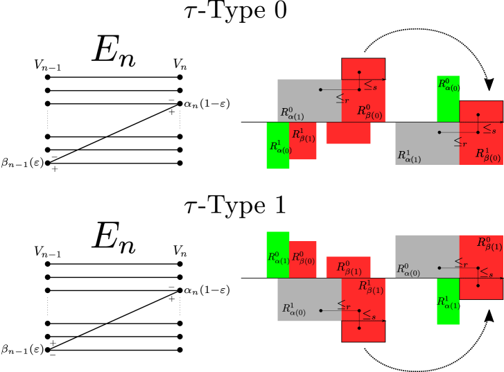
Figure 8. The edge set $E_{n}$ in the case that $\mathcal{P}^{n-1}(\pi,\lambda,\tau)$ is of $\tau$-type $\varepsilon$ in $\{0,1\}$. The $-$ and $+$ symbols indicate the orders at the vertices where there are more than one incoming or outgoing edges. When $\mathcal{P}^{n-1}(\pi,\lambda,\tau)$ is of $\tau$-type 0, the three dots in the rectangles $R^{0}_{\alpha(1)}$ and $R^{0}_{\beta(0)}$ used to define the orders $\leq_{r},\leq_{s}$. Indeed, the two dots sharing a $y$-coordinate sit on the same leaf of the horizontal leaf, making them right-tail-equivalent in $\mathcal{B}$. That $e_{\alpha_{n}(1)}<_{r}e_{n}$ in this case is dictated from the order on the leaf of the foliation containing those two points. This same order on the horizontal foliation happens in the case of $\tau$-type 0. The choice for the $\leq_{s}$ order comes from comparing two points on the same vertical leaf, and these take different forms depending on the type. This is evident from the two figures.

For $n>0$, let

(31) $$M_{n}=\left\{\begin{array}[]{ll}(\ref{eqn:Psi0})&\mbox{ if $\mathcal{P}^{n-1}(\pi,\lambda,\tau)$ is of $\tau$-type 0}\\ (\ref{eqn:Psi1})&\mbox{ if $\mathcal{P}^{n-1}(\pi,\lambda,\tau)$ is of $\tau$-type 1,}\end{array}\right.$$

and let $E_{n}$ be the edge set defined by $M_{n}$. In other words, there is an edge $e_{\alpha}$ in $E_{n}$ with $s_{n}(e_{\alpha})=\alpha$ in $V_{n-1}$ and $r_{n}(e_{\alpha})=\alpha$ in $V_{n}$, for each $\alpha$ in $\mathcal{A}$. We refer to such edges as horizontal. In addition, there is an edge $e_{n}$ in $E_{n}$ with $s_{n}(e_{n})=\beta_{n-1}(\varepsilon)$ and $r_{n}(e_{n})=\alpha_{n}(1-\varepsilon)$, if $\mathcal{P}^{n}(\pi,\lambda,\tau)$ is of type $\varepsilon$ in $\{0,1\}$, where $\alpha_{n}(\varepsilon)$ and $\beta_{n}(\varepsilon)$ are the corresponding symbols in the permutation in $\mathcal{P}^{n}(\pi,\lambda,\tau)$. Note that $\beta_{n}(\varepsilon)=\alpha_{n+1}(\varepsilon)$ depending on the type of $\mathcal{P}^{n}(\pi,\lambda,\tau)$.

We now move to define the orders $\leq_{r},\leq_{s}$ on $\mathcal{B}$. These will also depend on the $\tau$-type of $\mathcal{P}^{n-1}(\pi,\lambda,\tau)$. Since $|r_{n}^{-1}(\alpha)|=1$ for all $\alpha\neq\alpha_{n}(1-\varepsilon)$ and $n>0$, it suffices to define the order $\leq_{r}$ on $\{e_{n},e_{\alpha_{n}(1-\varepsilon)}\}=r^{-1}_{n}(\alpha_{n}(1-\varepsilon))$, depending of the type of $\mathcal{P}^{n-1}(\pi,\tau)$. We let

(32) $$e_{\alpha_{n}(1-\varepsilon)}<_{r}e_{n}$$

at each $r^{-1}_{n}(\alpha_{n}(1-\varepsilon))$, depending on the type. Since $|s_{n}^{-1}(\alpha)|=1$ for all $\alpha\neq\beta_{n-1}(\varepsilon)=\alpha_{n}(\varepsilon)$ and $n>0$ (here $\varepsilon$ is the type of $\mathcal{P}^{n-1}(\pi,\lambda,\tau)$), it suffices to define the order $\leq_{s}$ on $\{e_{n},e_{\beta_{n-1}(\varepsilon)}\}=s_{n}^{-1}(\beta_{n-1}(\varepsilon))$, depending of the type of $\mathcal{P}^{n-1}(\pi,\lambda,\tau)$. We define the orders

(33) $$\begin{array}[]{rl}e_{n}<_{s}e_{\alpha_{n}(1)}=e_{\beta_{n-1}(0)}&\mbox{ if $\mathcal{P}^{n-1}(\pi,\lambda,\tau)$ is of $\tau$-type 0,}\\ e_{\alpha_{n}(0)}=e_{\beta_{n-1}(1)}<_{s}e_{n}&\mbox{ if $\mathcal{P}^{n-1}(\pi,\lambda,\tau)$ is of $\tau$-type 1,}\end{array}$$

at $s_{n}^{-1}(\beta_{n-1}(\varepsilon))$. These choices define the positive half of $\mathcal{B}_{\pi,\lambda,\tau}$, see Figure 8 for a geometric justification for these choices.

The definition for the negative part will essentially be the same form as (31), if we use Proposition 12.9. Recall from the proof of Proposition 12.9 that if $(\pi,\lambda,\tau)=\mathcal{P}(\pi^{\prime},\lambda^{\prime},\tau^{\prime})$ is of $\lambda$-type $\varepsilon$, then $(\pi^{\prime},\lambda^{\prime},\tau^{\prime})=\mathcal{R}(\pi,\lambda,\tau)$ is of $\tau$-type $1-\varepsilon$. Thus, going by (31) for $n=0$ we can define $M_{0}$ as (20) if $(\pi,\lambda,\tau)$ is of $\lambda$ type $0$, and as (19) if $(\pi,\lambda,\tau)$ is of $\lambda$ type $1$. Extending for higher powers of $\mathcal{R}=\mathcal{P}^{-1}$, we get, for $n\leq 0$:

(34) $$M_{n}=\left\{\begin{array}[]{ll}(\ref{eqn:Psi1})&\mbox{ if $\mathcal{R}^{n}(\pi,\lambda,\tau)$ is of $\lambda$-type 0}\\ (\ref{eqn:Psi0})&\mbox{ if $\mathcal{R}^{n}(\pi,\lambda,\tau)$ is of $\lambda$-type 1}.\end{array}\right.$$

The orders are now similarly defined for the negative half: we extend the definitions using (32) and (33) depending on the $\tau$-type of $\mathcal{P}^{n-1}(\pi,\lambda,\tau)$, that is, depending on the $\lambda$-type of $\mathcal{R}^{n}(\pi,\lambda,\tau)$.

Remark 12.18.

1. Note that there are $2(|\mathcal{A}|-1)$ possible matrices that can appear as $\Psi$ in (31) and (34), all of which are invertible and of determinant 1. As such, we have for the AF algebras $A^{\pm}_{\mathcal{B}_{\pi,\lambda,\pi}}$ that the diagrams define,

   (35) $$K_{0}(A^{\pm}_{\mathcal{B}_{\pi,\lambda,\pi}})\cong\mathbb{Z}^{|\mathcal{A}|}\cong H_{1}(S(\pi,\lambda,\tau),\Sigma;\mathbb{Z}),$$

   which had already been proved in [Put92]. This does not, however, address the subtler issue of the natural order structure.

2. Given the definition of the Bratteli diagram $\mathcal{B}=\mathcal{B}_{\pi,\lambda,\tau}$ above, it is easy to identify some extreme elements at once: for any $\alpha$ in $\mathcal{A}$ the path $p_{\alpha}=(\dots,p_{\alpha}^{n-1},p_{\alpha}^{n},p_{\alpha}^{n+1},\dots)$ in $X_{\mathcal{B}}$ with $s_{n}(p_{\alpha}^{n})=\alpha$ and $r_{n}(p_{\alpha}^{n})=\alpha$ is in $X_{\mathcal{B}}^{r-min}$ and so $X_{\mathcal{B}}^{r-min}$ has exactly $|\mathcal{A}|$ elements, the horizontal paths in Figure 8.

Our next task is to define a state on the Bratteli diagram which we have just constructed. In fact, this is fairly simple: we let $(\pi_{n},\lambda_{n},\tau_{n})$ be $(\pi,\lambda,\tau)$ for $n=0$, $\mathcal{P}^{n}(\pi,\lambda,\tau)$ for $n>0$ and $\mathcal{R}^{-n}(\pi,\lambda,\tau)$ for $n<0$. We again let $h_{n}=\Omega_{\pi_{n}}(\tau_{n})$, which lies in $\mathbb{R}^{\mathcal{A}}$. For $\alpha$ in $\mathcal{A}=V_{n}$, we define $\nu_{r}(\alpha)=(\lambda_{n})_{\alpha}$ and $\nu_{s}(\alpha)=(h_{n})_{\alpha}$. It is a trivial matter to see that this is a state on $\mathcal{B}$.

It is a simple matter to see that these definitions mean that, for any $n>0$, a symbol $\alpha$ in $\mathcal{A}$ is the $\tau$-winner in RH induction, $\mathcal{P}^{n}$, if and only if the non-horizontal edge of $E_{n}$ has range equal to $\alpha$. Similarly, a symbol $\alpha$ is the $\lambda$-winner in Rauzy-Veech induction, $\mathcal{R}^{n}$, if and only if the non-horizontal edge of $E_{-n}$ has range equal to $\alpha$. This proves the following.

Proposition 12.19.

The Bratteli diagram $\mathcal{B}_{\pi,\lambda,\tau}$ satisfies the Keane condition if, for every $\alpha$ in $\mathcal{A}$, $|r_{n}^{-1}\{\alpha\}|>1$ for infinitely many negative integers $n$, and is RH-complete if and only if $|r_{n}^{-1}\{\alpha\}|>1$ for infinitely many positive integers $n$.

The next fact follows from [MMY05, §1.2.4] (see also [Ber21, Corollary 10]).

Proposition 12.20.

If $(\pi,\lambda,\tau)$ satisfies the Keane condition and is RH-complete, then $\mathcal{B}_{\pi,\lambda,\tau}$ is strongly simple.

The Keane condition allows us to describe the elements of $X^{ext}_{\mathcal{B}_{\pi,\lambda,\tau}}$ and even more, paths which are tail equivalent to these. To do so, we introduce some notation. Consider compatible representatives of the vertices of the Rauzy graph of $\pi$. That is, pick a representative $\pi=(\pi_{0},\pi_{1})$ of a vertex and consider the representatives of other classes which can be reached under finitely many steps of induction. Let $A_{\varepsilon}=\pi_{\varepsilon}(1)$, the first symbol of $\pi_{\varepsilon}$, and note that they are the first symbols in each representative in the Rauzy graph, that is, they are preserved under induction. Recall that there is an edge $e$ defined by the $\tau$-type of $(\pi,\lambda,\tau)$, which satisfies $s(e)=\beta(\varepsilon)$ and $r(e)=\alpha(1-\varepsilon)$ whenever the $\tau$-type is $\varepsilon$ (Figure 8).

Proposition 12.21.

Suppose that $(\pi,\lambda,\tau)$ satisfies the Keane condition, is RH-complete and that $x$ is an infinite path in $\mathcal{B}_{\pi,\lambda,\tau}$.

1. Suppose there is $n_{0}$ such that $x_{n}$ is $r$-minimal, for all $n\leq n_{0}$. Then $x_{n}$ is horizontal, for all $n\leq n_{0}$. In particular, $X^{r-min}_{\mathcal{B}_{\pi,\lambda,\tau}}$ consists of the $|\mathcal{A}|$ infinite horizontal paths.

2. If $x$ is in $X^{r-max}_{\mathcal{B}_{\pi,\lambda,\tau}}$, then $x_{n}$ is not horizontal, for infinitely many $n>0$.

3. Suppose that there is an integer $n_{0}$ such that $x_{n}$ is $s$-maximal for all $n\geq n_{0}$. Then there exists $m_{0}\geq n_{0}$ such that $r(x_{n})=s(x_{n})=A_{0}$, for all $n\geq m_{0}$.

4. Suppose that there is an integer $n_{0}$ such that $x_{n}$ is $s$-minimal for all $n\geq n_{0}$. Then there exists $m_{0}\geq n_{0}$ such that $r(x_{n})=s(x_{n})=A_{1}$, for all $n\geq m_{0}$.

Proof.

The first part follows easily (even without the Keane condition) from the fact that if $x_{n}$ is $r$-minimal, then it is horizontal, by the definition of $\leq_{r}$.

For the second part, suppose that $x_{n}$ is horizontal for all $n>0$. From the BK condition, there $n>1$ with $|r^{-1}(r(x_{n})|>1$. The definition of $\leq_{r}$ implies that $x_{n}$ is not $r$-maximal.

The last two parts are more subtle.

Observe that $A_{\varepsilon}\neq\beta(\varepsilon)$, since by definition $\beta(\varepsilon)$ is the symbol to the right of another symbol, and $A_{\varepsilon}$ is never to the right of another symbol. Thus there is no non-horizontal edge $e$ defined by the graph with the property that $s(e)=A_{\varepsilon}$ when the data is of type $\varepsilon$. This means that whenever there is a non-horizontal edge $e$ with $s(e)=A_{0}$, then this corresponds to type $1$, and so it is $s$-max, and likewise if there is a non-horizontal edge $e$ with $s(e)=A_{1}$, then this corresponds to type $0$, and so it is $s$-min. It follows that the constant path $\{A_{0}\}$ is $s$-min while the constant path $\{A_{1}\}$ is $s$-max, and both of these paths are also $r$-min.

For a set $V\subseteq V_{n}$, we define

$$Q(V)=\{s(e)\mid e\in E_{n}\mbox{ is $s$-minimal and }r(e)\in V\}.$$

For $V\subseteq V_{n}$ we will denote $Q^{m}(V)\subseteq V_{n-m}$ the image of the composition of $Q$ $m$ times. We first observe that if $\alpha$ is in $Q^{m}(\{A_{0}\})\subseteq V_{n-m}$, then there is an $s$-min path in $E_{n-m,n}$ with $s(p)=\alpha$ and $r(p)=A_{0}$.

Lemma 12.22.

For any $1\leq i<d$, if $V=\{\alpha^{0}_{1},\ldots,\alpha^{0}_{i}\}$, then $Q(V)$ equals one of $\{(\alpha^{\prime})^{0}_{1},\ldots,(\alpha^{\prime})^{0}_{i}\}$ or $\{(\alpha^{\prime})^{0}_{1},\ldots,(\alpha^{\prime})^{0}_{i+1}\}$ Moreover, if $(\pi,\lambda,\tau)$ is $\tau$-type 0 and $\alpha(1)$ is in $V$, then the latter holds.

Proof.

The first case to consider is when $(\pi,\lambda,\tau)$ is $\tau$-type $1$. In this case, every $s$-minimal edge in $E_{n}$ is horizontal and so $Q(V)=V$, for any set $V$. On the other hand, $(\alpha^{\prime})^{0}=\alpha^{0}$ and so the conclusion holds, with the first of the two cases.

We now assume $(\pi,\lambda,\tau)$ is $\tau$-type $0$. Suppose $\alpha(1)=\alpha^{0}_{k}$, for some $1\leq k\leq d$. There are two cases to consider. The first is that $\alpha(1)$ is not in $V$. In other words, $\alpha(1)=\alpha_{j}^{0}$, for some $j>i$. In this case, the horizontal edge to each element of $V$ is also $s$-minimal so $Q(V)=V$. Moreover, the change in $\beta^{0}$ from $\alpha^{0}$ only occurs in entries greater than $k$. In other words, we have $\{(\alpha^{\prime})^{0}_{1},\ldots,(\alpha^{\prime})^{0}_{i}\}=\{\alpha^{0}_{1},\ldots,\alpha^{0}_{j}\}=V$ and $Q(V)=V$.

Now, we suppose that $\alpha(1)$ is in $V$. In other words, $\alpha(1)=\alpha_{j}^{0}$, for some $j\leq i$. In this case, we have the non-horizontal $s$-min edge goes from $\alpha(0)$ to $\alpha(1)$. Observe that because $i<d$, $\alpha(0)$ is not in $V$. It follows that $Q(V)=V\cup\{\alpha(0)\}$. On the other hand, $(\alpha^{\prime})^{0}$ is obtained from $\alpha^{0}$ by inserting $\alpha(0)$ to the right of $\alpha(1)$ and moving the entries to the right one more space to the right. In other words, we have $\{(\alpha^{\prime})^{0}_{1},\ldots,(\alpha^{\prime})^{0}_{i+1}\}=V\cup\{\alpha(0)\}$ and we are done. ∎

∎

Proposition 12.23.

If $(\pi,\lambda,\tau)$ is such that, $|r_{n}^{-1}\{A_{0}\}|>1$ for infinitely many $n>0$, then any $x$ in $X_{\mathcal{B}_{\pi,\lambda,\tau}}$ such that there is some $n_{0}$ such $x_{n}$ is $s$-minimal, for all $n\geq n_{0}$, there is $n_{1}$ such that $x_{n}$ is the horizontal edge from $A_{0}$ to itself, for all $n\geq n_{1}$. In particular, $I_{\mathcal{B}_{\pi,\lambda,\tau}}^{+}=1$ with $x_{1}$ being the infinite horizontal path through $A_{0}$. Similarly, if $(\pi,\lambda,\tau)$ is such that, $|r_{n}^{-1}\{A_{1}\}|>1$ for infinitely many $n>0$, then any $x$ in $X_{\mathcal{B}_{\pi,\lambda,\tau}}$ such that there is some $n_{0}$ such $x_{n}$ is $s$-maximal, for all $n\geq n_{0}$, there is $n_{1}$ such that $x_{n}$ is the horizontal edge from $A_{1}$ to itself, for all $n\geq n_{1}$. In particular, $J_{\mathcal{B}_{\pi,\lambda,\tau}}^{+}=1$ with $x_{2}$ being the infinite horizontal path through $A_{0}$.

Proof.

We prove the first statement only. Choose $n_{1}>n_{0}$ so that $|r_{n}^{-1}\{A_{0}\}|>1$, for at least $|\mathcal{A}|$ values of $n$ between $n_{0}$ and $n_{1}$. If we then consider $A_{0}$ as a vertex in $V_{n_{1}}$, and apply $Q$ successively to $V=\{A_{0}\}$, there will be at least $|\mathcal{A}|$ times when $Q^{m}(V)$ is strictly larger then $V$. For some some $n_{0}\leq n\leq n_{1}$, we have $Q^{n_{1}-n}(V)=V_{n}$. It follows that every $s$-minimal starting in $V_{n}$ will have range equal to $A_{0}$. Also, any $s$-minimal path starting at $A_{0}$ will be horizontal. As $n\geq n_{0}$, $x$ satisfies both properties and the conclusion follows. ∎

Theorem 12.24.

If $(\pi,\lambda,\tau)$ in $\mathcal{V}_{\mathcal{C}}$ satisfies the Keane condition and is RH-complete, then $\mathcal{B}_{\pi,\lambda,\tau}$ satisfies the standard conditions of Definition 6.2.

Proof.

We have already seen that $\mathcal{B}_{\pi,\lambda,\tau}$ is strongly simple in Proposition 12.20. It is clearly finite rank since $\#V_{n}=\#\mathcal{A}$, for all integers $n$.

We finally verify the third condition, starting with considering $(X_{\mathcal{B}}^{s-min}\cup X_{\mathcal{B}}^{s-max})\cap\partial_{r}X_{\mathcal{B}}$. We know from Proposition 12.23 that $(X_{\mathcal{B}}^{s-min}$ and $X_{\mathcal{B}}^{s-max})$ consist of $x_{1}$ and $x_{2}$, the horizontal paths through $A_{0}$ and $A_{1}$, respectively, and hence are both in $X_{\mathcal{B}}^{r-min}$ which is excluded from $\partial_{r}X_{\mathcal{B}}$, by definition.

We now consider $(X_{\mathcal{B}}^{r-min}\cup X_{\mathcal{B}}^{r-max})\cap\partial_{s}X_{\mathcal{B}}$. Again Proposition 12.23 implies that $\partial_{s}X_{\mathcal{B}}$ is contained in $T^{+}(x_{1})$ and $T^{+}(x_{2})$. The only paths which also lie in $X^{r-min}_{\mathcal{B}}$ are the horizontal paths $x_{1}$ and $x_{2}$, which are excluded from $\partial_{s}X_{\mathcal{B}}$, by definition. If $x$ is in $T^{+}(x_{1})$ and $X^{r-max}_{\mathcal{B}}$, then $x_{n}$ is the horizontal edge from $A_{0}$ to itself for all $n\geq n_{0}$. By RH-completeness, there is some $n\geq n_{0}$ with $|r_{n}^{-1}\{A_{0}\}|>1$, which means that $x_{n}$ is not $r$-maximal, a contradiction. The same argument shows $T^{+}(x_{2})\cap X^{r-max}_{\mathcal{B}}$ is empty. ∎

12.7. Flatness of $\mathcal{B}_{\pi,\lambda,\tau}$

In this section, we will prove the following flatness property of $\mathcal{B}_{\pi,\lambda,\tau}$.

Theorem 12.25.

If $(\pi,\lambda,\tau)$ in $\mathcal{V}_{\mathcal{C}}$ satisfies the Keane condition and is RH-complete, then $\Sigma_{\mathcal{B}_{\pi,\lambda,\tau}}=\varnothing$.

Denote by $x_{\varepsilon}=\{A_{\varepsilon}\}$ the corresponding $s$-min/max paths from Proposition 12.21. Then $T^{+}(x_{\varepsilon})$ is linearly ordered by $\leq_{r}$ and $\Delta_{s}:T^{+}(x_{\varepsilon})\setminus\{x_{\varepsilon}\}\rightarrow T^{+}(x_{1-\varepsilon})\setminus\{x_{1-\varepsilon}\}$ is a bijection.

Lemma 12.26.

If $\Delta_{s}$ preserves $\leq_{r}$, then $\Sigma_{\mathcal{B}}=\varnothing$.

Proof.

Let $x\in\partial X_{\mathcal{B}}$ and suppose $\Delta_{r}(x)$ is the $r$-successor of $x$. Then $\Delta_{s}\circ\Delta_{r}(x)$ is the $r$-successor of $\Delta_{s}(x)$, that is $\Delta_{r}\circ\Delta_{s}(x)=\Delta_{s}\circ\Delta_{r}(x)$. ∎

For every $n$, $E_{n}$ has an edge which is not $s$-max, call it $y_{n}$ and an edge $z_{n}$ which is not $s$-min. These are the edges $\{y_{n},z_{n}\}=s^{-1}(v_{\beta_{n-1}(\varepsilon)})$. Define

(36) $$\begin{split}Y_{n}&=\left\{x\in X_{\mathcal{B}}\mid x_{n}=y_{n}\mbox{ and }x_{i}\mbox{ is $s$-max for all }i>n\right\}\\ Z_{n}&=\left\{x\in X_{\mathcal{B}}\mid x_{n}=z_{n}\mbox{ and }x_{i}\mbox{ is $s$-min for all }i>n\right\}.\end{split}$$

Note that $\Delta_{s}:Y_{n}\rightarrow Z_{n}$ is a bijection for every $n$. Moreover, by definition, we also have that

$$T^{+}(x_{0})\setminus\{x_{0}\}=\bigsqcup_{n}Y_{n}\hskip 28.90755pt\mbox{ and }\hskip 28.90755ptT^{+}(x_{1})\setminus\{x_{1}\}=\bigsqcup_{n}Z_{n}$$

so if $Y_{n}\leq_{r}Y_{n+1}$ and $Z_{n}\leq_{r}Z_{n+1}$, for all $n$, then $\Delta_{s}:T^{+}(x_{\varepsilon})\setminus\{x_{\varepsilon}\}\rightarrow T^{+}(x_{1-\varepsilon})\setminus\{x_{1-\varepsilon}\}$ preserves $\leq_{r}$.

Proposition 12.27.

$Y_{n}\leq_{r}Y_{n+1}$

Let $x=\{e_{i}\}$ be in $Y_{n}$ and $x^{\prime}=\{e^{\prime}_{i}\}$ be in $Y_{n+1}$. Let $\ell>n$ be the smallest integer where $r(e_{i})=r(e^{\prime}_{i})$. We will show that $e_{\ell}\leq_{r}e_{\ell}^{\prime}$. We first treat two simple cases.

Lemma 12.28.

If $E_{n},E_{n+1}$ are respectively of $\tau$-type 0,0 or 1,0, then $\ell=n+1$ and $e_{n+1}\leq_{r}e_{n+1}^{\prime}$.

Proof.

If they are of type 0,0, it is immediate to check that $(e_{n},e_{n+1})$ is the concatenation of the $s$-min path from $\beta(0)$ to $\alpha(0)$ followed by the horizontal edge $e_{\alpha(0)}$, whereas $e_{n+1}^{\prime}$ is the $s$-min path from some vertex to $v_{\alpha(0)}$, meaning that $r(e_{n+1})=r(e_{n+1}^{\prime})$. Since horizontal paths are always $r$-min, it follows that $e_{n+1}\leq_{r}e_{n+1}^{\prime}$.

If they are of type 1,0, then it is immediate to check that $(e_{n},e_{n+1})$ is the horizontal path associated with symbol $\beta(1)$, whereas $e_{n+1}^{\prime}$ is the $s$-min path from some vertex to $\beta(1)=r(e_{n+1})$. Again, since horizontal paths are always $r$-min, it follows that $e_{n+1}\leq_{r}e_{n+1}^{\prime}$. ∎

Thus we are left to inspect the cases where $E_{n},E_{n+1}$ are respectively of types 0,1 or 1,1.

Lemma 12.29.

Suppose $E_{n},E_{n+1}$ are respectively of types 0,1 or 1,1. For $n+1\leq i<\ell-1$, if $r(e_{i})=\gamma$ and $r(e_{i}^{\prime})=\gamma^{\prime}$, then the symbol $\gamma$ is immediately to the left of $\gamma^{\prime}$ on the bottom row of the permutation defined by $\mathcal{P}^{i}(\pi,\lambda,\tau)$.

Before proving this lemma, let us prove the proposition assuming the lemma.

Proof of Proposition 12.27 assuming Lemma 12.29.

First note that if $r(e_{\ell})=r(e_{\ell}^{\prime})$, then
$\mathcal{P}^{\ell-1}(\pi,\lambda,\tau)$ is of $\tau$-type 1, as this is the only way that we can have a non-horizontal $s$-max edge in $E_{\ell}$. If $r(e_{\ell-1})=\gamma$ and $r(e^{\prime}_{\ell-1})=\gamma^{\prime}$ and $\gamma$ is immediately to the left of of $\gamma^{\prime}$, then by the definition ( 31) of $M_{\ell}$, the non-horizontal edge goes from $\gamma^{\prime}$ in $V_{\ell-1}$ to $\gamma$ in $V_{\ell}$, and so $e_{\ell}\leq_{r}e_{\ell}^{\prime}$, showing that $Y_{n}\leq_{r}Y_{n+1}$. ∎

We now move to prove Lemma 12.29. To get us started, we have the following.

Lemma 12.30.

If $E_{n},E_{n+1}$ are respectively of $\tau$-type 0,1 or 1,1, then $\ell>n+1$ and the permutation associated to $\mathcal{P}^{n+1}(\pi,\lambda,\tau)$ is of the form

(37) $$\left(\begin{array}[]{lr}\cdots&\cdots\\ \cdots&\gamma\gamma^{\prime}\end{array}\right)$$

for some $\gamma,\gamma^{\prime}$ in $\mathcal{A}$, then $r(e_{n+1})=\gamma$ and $r(e_{n+1}^{\prime})=\gamma^{\prime}$.

Proof.

Suppose they are respectively of type 0,1. Then the sequence of permutations are of the form

$$\left(\begin{array}[]{r}\cdots\alpha(1)\beta(0)\cdots\alpha(0)\\ \cdots\alpha(0)\beta(1)\cdots\alpha(1)\end{array}\right)\mapsto\left(\begin{array}[]{r}\cdots\alpha(1)\cdots\alpha(0)\beta(0)\\ \cdots\beta(0)\beta^{\prime}(1)\cdots\alpha(1)\end{array}\right)\mapsto\left(\begin{array}[]{r}\cdots\alpha(1)\cdots\alpha(0)\beta(0)\\ \cdots\beta(0)\cdots\alpha(1)\beta^{\prime}(1)\end{array}\right),$$

assuming $\beta(0)\neq\alpha(0)$ and $\beta^{\prime}(1)\neq\alpha(1)$. Now, by definition, $(e_{n},e_{n+1})$ is the concatenation of the edge from $\beta(0)$ to the vertex $\alpha(1)$ followed by the horizontal edge associated to the symbol $\alpha(1)$, and so $\gamma=\alpha(1)$, whereas $e_{n+1}^{\prime}$ is the horizontal edge associated to the symbol $\beta^{\prime}(1)$ and $\gamma^{\prime}=\beta^{\prime}(1)$.

Note that it cannot be the case that both $\beta(0)=\alpha(0)$ and $\beta^{\prime}(1)=\alpha(1)$ as this would make the permutation irreducible. Now, if $\beta(0)=\alpha(0)$ and $\beta^{\prime}(1)\neq\alpha(1)$, then the sequence of permutations is of the form

$$\left(\begin{array}[]{r}\cdots\alpha(1)\alpha(0)\\ \cdots\alpha(0)\beta(1)\cdots\alpha(1)\end{array}\right)\mapsto\left(\begin{array}[]{r}\cdots\alpha(1)\alpha(0)\\ \cdots\alpha(0)\beta(1)\cdots\alpha(1)\end{array}\right)\mapsto\left(\begin{array}[]{r}\cdots\cdots\cdots\alpha(1)\alpha(0)\\ \cdots\alpha(0)\cdots\alpha(1)\beta(1)\end{array}\right).$$

Here, $(e_{n},e_{n+1})$ is the concatenation of the edge from $\alpha(0)$ to $\alpha(1)$ followed by the horizontal edge associated to the symbol $\alpha(1)$, and so $\gamma=\alpha(1)$, whereas $e_{n+1}^{\prime}$ is the horizontal edge associated to the symbol $\beta(1)$ and $\gamma^{\prime}=\beta(1)$, and the result also holds here.

If $\beta(0)\neq\alpha(0)$ and $\beta^{\prime}(1)=\alpha(1)$, then the sequence of permutations is of the form

$$\left(\begin{array}[]{r}\cdots\alpha(1)\beta(0)\cdots\alpha(0)\\ \cdots\alpha(0)\beta(1)\cdots\alpha(1)\end{array}\right)\mapsto\left(\begin{array}[]{r}\cdots\alpha(1)\cdots\alpha(0)\beta(0)\\ \cdots\beta(0)\alpha(1)\end{array}\right)\mapsto\left(\begin{array}[]{r}\cdots\alpha(1)\cdots\alpha(0)\beta(0)\\ \cdots\beta(0)\alpha(1)\end{array}\right),$$

Here, $(e_{n},e_{n+1})$ is the concatenation of the edge from $\beta(0)$ to $\alpha(1)$ followed by the (non-horizontal) path from $\beta^{\prime}(1)=\alpha(1)$ to $\beta(0)$, whereas $e_{n+1}^{\prime}$ is the horizontal edge associated to the symbol $\alpha(1)$, and so $(\gamma,\gamma^{\prime})=(\beta(0),\alpha(1))$ and the case of types 0,1 is proved.

Now suppose they are respectively of type 1,1. Then the sequence of permutations are of the form

$$\left(\begin{array}[]{r}\cdots\alpha(1)\beta(0)\cdots\alpha(0)\\ \cdots\alpha(0)\beta(1)\cdots\alpha(1)\end{array}\right)\mapsto\left(\begin{array}[]{r}\cdots\beta(1)\beta^{\prime}(0)\cdots\alpha(0)\\ \cdots\alpha(0)\beta^{\prime}(1)\cdots\alpha(1)\beta(1)\end{array}\right)\mapsto\left(\begin{array}[]{r}\cdots\cdots\cdots\cdots\alpha(0)\\ \cdots\alpha(0)\cdots\alpha(1)\beta(1)\beta^{\prime}(1)\end{array}\right),$$

assuming $\beta(1)\neq\alpha(1)$ (note that $\beta^{\prime}(1)\neq\beta(1)$ as equality would imply that $\alpha(0)=\alpha(1)$ making the original permutation reducible). Now, by definition, $e_{n+1}^{\prime}$ is the horizontal edge associated to the symbol $\beta^{\prime}(1)\neq\beta(1)$, whereas $(e_{n},e_{n+1})$ is the concatenation of the horizontal edge associated to the symbol $\beta(1)$ followed by the horizontal edge associated to the same symbol, $\beta(1)$, and so $\gamma=\beta(1)$ and $\gamma^{\prime}=\beta^{\prime}(1)$.

If $\alpha(1)=\beta(1)$, then the starting permutation is fixed under $\mathcal{P}$ and $\mathcal{P}^{2}$ (under $\tau$-type 1) and it is of the form

$$\left(\begin{array}[]{r}\cdots\alpha(1)\beta(0)\cdots\alpha(0)\\ \cdots\alpha(0)\alpha(1)\end{array}\right).$$

In this case, $(e_{n},e_{n+1})$ is the concatenation of the horizontal edge with symbol $\beta(1)=\alpha(1)$ followed by the (non-horizontal) edge from $\beta(1)$ to $\alpha(0)$, whereas $e_{n+1}^{\prime}$ is the horizontal edge with symbol $\beta(1)=\alpha(1)$. So $(\gamma,\gamma^{\prime})=(\alpha(0),\alpha(1))$ in this case and the lemma is proved. ∎

Proof of Lemma 12.29.

Given Lemma 12.30, we only need to prove that this property does not change when applying $\mathcal{P}$. Now, if $E_{n+2}$ is of $\tau$-type $0$ then $e_{n+2},e_{n+2}^{\prime}$ are both horizontal edges and the condition in the permutation in Lemma 12.30 does not change. In general, going through an edge set of $\tau$-type 0 does not change anything: if $e_{i},e_{i}^{\prime}$ are horizontal edges and have symbols $\gamma,\gamma^{\prime}$, respectively, and $\gamma$ sits to the left of $\gamma^{\prime}$ in the bottom row, and $E_{i}$ is of $\tau$-type 0, then the new permutation will have $\gamma$ and $\gamma^{\prime}$ in the same relative positions in the bottom row. Thus it is only when we get to an edge set $E_{i}$ of $\tau$-type 1 that things may change.

Let $e_{i},e_{i}^{\prime}\in E_{i}$ have $r(e_{i})=v_{\gamma}$ and $r(e_{i}^{\prime})=v_{\gamma^{\prime}}$ and such that the permutation of $\mathcal{P}^{i}(\pi,\lambda,\tau)$ is of $\tau$-type 1 and has $\gamma$ immediately to the left of $\gamma^{\prime}$ on the bottom row. Then either

1. $\mathcal{P}^{i+1}(\pi,\lambda,\tau)$ has $\gamma,\gamma^{\prime}$ in the same positions on the bottom row,

2. $\mathcal{P}^{i+1}(\pi,\lambda,\tau)$ has $\gamma,\gamma^{\prime}$ shifted on spot to the left on the bottom row,

3. $\mathcal{P}^{i+1}(\pi,\lambda,\tau)$ has $\gamma$ at the end of the bottom row, or

4. $\mathcal{P}^{i+1}(\pi,\lambda,\tau)$ has $\gamma^{\prime}$ at the end of the bottom row.

We now treat each case. In case (i), then the bottom row of the permutation in $\mathcal{P}^{i+1}(\pi,\lambda,\tau)$ differs from the bottom row of that of $\mathcal{P}^{i}(\pi,\lambda,\tau)$ on some symbols to the right of $\gamma^{\prime}$. This means that $r(e_{i+1})=v_{\gamma}$ and $r(e_{i+1})=v_{\gamma^{\prime}}$ and so the condition is preserved. If case (ii) holds, then that means that a symbol to the left of $\gamma$ got sent to the end of the bottom row when going from $\mathcal{P}^{i}(\pi,\lambda,\tau)$ to $\mathcal{P}^{i+1}(\pi,\lambda,\tau)$. This again implies that $r(e_{i+1})=v_{\gamma}$ and $r(e_{i+1})=v_{\gamma^{\prime}}$ and so the condition is also preserved.

Now suppose that case (iii) holds. Then the non-horizontal edge $e_{*}\in E_{i+1}$ goes from $\beta_{i}(1)=\gamma$ to $\alpha_{i}(0)\neq\gamma^{\prime}$. This edge is $s$-max and so since $s(e_{*})=r(e_{i})$ we have that $e_{*}=e_{i+1}$. Since $\gamma$ got moved to the end of the row, we have that $\gamma^{\prime}$ sits immediately to the right of $\alpha_{i}(0)$. Since $r(e_{i+1})=\alpha_{i}(0)$, the condition is preserved.

Finally, in case (iv), since $\gamma^{\prime}$ gets moved to the end of the bottom row this means that the non-horizontal edge in $E_{i+1}$ goes from $\gamma^{\prime}$ to $\gamma$ and so $r(e_{i+1})=r(e_{i+1}^{\prime})$. This can only happen if $i+1=\ell$ by the definition of $\ell$, but we are assuming $i<\ell-1$, so this cannot happen. We have proved that the condition is preserved under every case. ∎

We now move to prove that $Z_{n}\leq_{r}Z_{n+1}$. It is done through the same arguments used to show that $Y_{n}\leq_{r}Y_{n+1}$ (Proposition 12.21).

Proposition 12.31.

$Z_{n}\leq_{r}Z_{n+1}$

Let $x=\{e_{i}\}$ be in $Z_{n}$ and $x^{\prime}=\{e^{\prime}_{i}\}$ be in $Z_{n+1}$. Let $\ell>n$ be the smallest integer where $r(e_{i})=r(e^{\prime}_{i})$. We will show that $e_{\ell}\leq_{r}e_{\ell}^{\prime}$.

Lemma 12.32.

If $E_{n},E_{n+1}$ are respectively of $\tau$-type 0,1 or 1,1, then $\ell=n+1$ and $e_{n+1}\leq_{r}e_{n+1}^{\prime}$.

Proof.

If they are of type 0,1, it is immediate to check that $(e_{n},e_{n+1})$ is the concatenation of the $s$-max path from $\beta(0)$ to $\beta(0)$ followed by the horizontal edge $e_{\beta(0)}$, whereas $e_{n+1}^{\prime}$ is the (non-horizontal) $s$-max path from some vertex to $\beta(0)$, meaning that $r(e_{n+1})=r(e_{n+1}^{\prime})$. Since horizontal paths are always $r$-min, it follows that $e_{n+1}\leq_{r}e_{n+1}^{\prime}$.

If they are of type 1,1, then it is immediate to check that $(e_{n},e_{n+1})$ is the non-horizontal horizontal path from $\beta(1)$ to $\alpha(0)$ followed by the horizontal path associated to the symbol $\alpha(0)$, whereas $e_{n+1}^{\prime}$ is the $s$-max path from some vertex to $v_{\alpha(0)}=r(e_{n+1})$. Again, since horizontal paths are always $r$-min, it follows that $e_{n+1}\leq_{r}e_{n+1}^{\prime}$. ∎

We now inspect the cases where $E_{n},E_{n+1}$ are respectively of types 0,0 or 1,0.

Lemma 12.33.

Suppose $E_{n},E_{n+1}$ are respectively of types 0,0 or 1,0. For $n+1\leq i<\ell-1$, if $r(e_{i})=v_{\gamma}$ and $r(e_{i}^{\prime})=\gamma^{\prime}$, then the symbol $\gamma$ is immediately to the left of $\gamma^{\prime}$ on the top row of the permutation defined by $\mathcal{P}^{i}(\pi,\lambda,\tau)$.

Before proving this lemma, let us prove the proposition assuming the lemma.

Proof of Proposition 12.31 assuming Lemma 12.33.

First note that if $r(e_{\ell})=r(e_{\ell}^{\prime})$ then $\mathcal{P}^{\ell-1}(\pi,\lambda,\tau)$ is of $\tau$-type 0, as this is the only way that we can have a non-horizontal $s$-min edge in $E_{\ell}$. If $r(e_{\ell-1})=\gamma$ and $r(e^{\prime}_{\ell-1})=\gamma^{\prime}$ and $\gamma$ is immediately to the left of of $\gamma^{\prime}$, then by the definition (31) of $M_{\ell}$, the non-horizontal edge goes from $\gamma^{\prime}$ in $V_{\ell-1}$ to $\gamma$ in $V_{\ell}$, and so $e_{\ell}\leq_{r}e_{\ell}^{\prime}$, showing that $Z_{n}\leq_{r}Z_{n+1}$. ∎

To prove Lemma 12.33, we begin by proving the analog of Lemma 12.30.

Lemma 12.34.

If $E_{n},E_{n+1}$ are respectively of $\tau$-type 0,0 or 1,0, then $\ell>n+1$ and the permutation associated to $\mathcal{P}^{n+1}(\pi,\lambda,\tau)$ is of the form

(38) $$\left(\begin{array}[]{lr}\cdots&\gamma\gamma^{\prime}\\ \cdots&\cdots\end{array}\right),$$

for some $\gamma,\gamma^{\prime}$ in $\mathcal{A}$, then $r(e_{n+1})=\gamma$ and $r(e_{n+1}^{\prime})=\gamma^{\prime}$.

Proof.

Suppose they are respectively of type 0,0. Then the sequence of permutations are of the form

$$\left(\begin{array}[]{r}\cdots\alpha(1)\beta(0)\cdots\alpha(0)\\ \cdots\alpha(0)\beta(1)\cdots\alpha(1)\end{array}\right)\mapsto\left(\begin{array}[]{r}\cdots\alpha(1)\beta^{\prime}(0)\cdots\alpha(0)\beta(0)\\ \cdots\alpha(0)\beta(1)\cdots\alpha(1)\end{array}\right)\mapsto\left(\begin{array}[]{r}\cdots\alpha(1)\cdots\alpha(0)\beta(0)\beta^{\prime}(0)\\ \cdots\cdots\cdots\cdots\alpha(1)\end{array}\right),$$

assuming $\beta(0)\neq\alpha(0)$ (note that $\beta^{\prime}(0)\neq\beta(0)$ as equality would imply that $\alpha(0)=\alpha(1)$ making the original permutation reducible). Now, by definition, $e_{n+1}^{\prime}$ is the horizontal edge associated to the symbol $\beta^{\prime}(0)\neq\beta(0)$, whereas $(e_{n},e_{n+1})$ is the concatenation of the horizontal edge associated to the symbol $\beta(0)$ followed by the horizontal edge associated to the same symbol, $\beta(0)$, and so $\gamma=\beta(0)$ and $\gamma^{\prime}=\beta^{\prime}(0)$.

If $\alpha(0)=\beta(0)$, then the starting permutation is fixed under $\mathcal{P}$ and $\mathcal{P}^{2}$ (under $\tau$-type 0) and it is of the form

$$\left(\begin{array}[]{r}\cdots\alpha(1)\alpha(0)\\ \cdots\alpha(0)\beta(1)\cdots\alpha(1)\end{array}\right).$$

In this case $(e_{n},e_{n+1})$ is the concatenation of horizontal edge with symbol $\beta(0)=\alpha(0)$ followed by the (non-horizontal) edge from $\beta(0)$ to $\alpha(1)$, whereas $e_{n+1}^{\prime}$ is the horizontal edge with symbol $\beta(0)=\alpha(0)$. So $(\gamma,\gamma^{\prime})=(\alpha(1),\alpha(0))$ in this case and the lemma is proved for type 0,0.

If we have type 1,0, then the sequence of permutations are of the form

$$\left(\begin{array}[]{r}\cdots\alpha(1)\beta(0)\cdots\alpha(0)\\ \cdots\alpha(0)\beta(1)\cdots\alpha(1)\end{array}\right)\mapsto\left(\begin{array}[]{r}\cdots\beta(1)\beta^{\prime}(0)\cdots\alpha(0)\\ \cdots\alpha(0)\cdots\alpha(1)\beta(1)\end{array}\right)\mapsto\left(\begin{array}[]{r}\cdots\beta(1)\cdots\alpha(0)\beta^{\prime}(0)\\ \cdots\alpha(0)\cdots\alpha(1)\beta(1)\end{array}\right),$$

assuming $\beta(1)\neq\alpha(1)$ and $\beta^{\prime}(0)\neq\alpha(0)$. Now, by definition, $(e_{n},e_{n+1})$ is the concatenation of the edge from $\beta(1)$ to the vertex $\alpha(0)$ followed by the horizontal edge associataed to the symbol $\alpha(0)$, and so $\gamma=\alpha(0)$, whereas $e_{n+1}^{\prime}$ is the horizontal edge associated to the symbol $\beta^{\prime}(0)$ and $\gamma^{\prime}=\beta^{\prime}(0)$.

Note that it cannot be the case that both $\beta(1)=\alpha(1)$ and $\beta^{\prime}(0)=\alpha(0)$ as this would make the permutation irreducible. Now, if $\beta(1)=\alpha(1)$ and $\beta^{\prime}(0)\neq\alpha(0)$, then the sequence of permutations is of the form

$$\left(\begin{array}[]{r}\cdots\alpha(1)\beta(0)\cdots\alpha(0)\\ \cdots\alpha(0)\alpha(1)\end{array}\right)\mapsto\left(\begin{array}[]{r}\cdots\alpha(1)\beta(0)\cdots\alpha(0)\\ \cdots\alpha(0)\alpha(1)\end{array}\right)\mapsto\left(\begin{array}[]{r}\cdots\alpha(1)\cdots\alpha(0)\beta(0)\\ \cdots\cdots\cdots\alpha(0)\alpha(1)\end{array}\right).$$

Here ,$(e_{n},e_{n+1})$ is the concatenation of the edge from $\alpha(1)$ to $\alpha(0)$ followed by the horizontal edge associated to the symbol $\alpha(0)$, and so $\gamma=\alpha(0)$, whereas $e_{n+1}^{\prime}$ is the horizontal edge associated to the symbol $\beta(0)$ and $\gamma^{\prime}=\beta(0)$, and the result also holds here.

Finally, if $\beta(1)\neq\alpha(1)$ and $\beta^{\prime}(0)=\alpha(0)$, then the sequence of permutations is of the form

$$\left(\begin{array}[]{r}\cdots\alpha(1)\beta(0)\cdots\alpha(0)\\ \cdots\alpha(0)\beta(1)\cdots\alpha(1)\end{array}\right)\mapsto\left(\begin{array}[]{r}\cdots\beta(1)\alpha(0)\\ \cdots\alpha(0)\cdots\alpha(1)\beta(1)\end{array}\right)\mapsto\left(\begin{array}[]{r}\cdots\beta(1)\alpha(0)\\ \cdots\alpha(0)\cdots\alpha(1)\beta(1)\end{array}\right),$$

Here $(e_{n},e_{n+1})$ is the concatenation of the edge from $\beta(1)$ to $\alpha(0)$ followed by the (non-horizontal) path from $\beta^{\prime}(0)=\alpha(0)$ to $\beta(1)$, whereas $e_{n+1}^{\prime}$ is the horizontal edge associated to the symbol $\alpha(0)$, and so $(\gamma,\gamma^{\prime})=(\beta(0),\alpha(1))$ and the case of types 0,1 is proved. ∎

Proof of Lemma 12.33.

The proof of this Lemma follows the same argument as the proof of Lemma 12.29 except $\tau$-type $\varepsilon$ has to be replaced with type $1-\varepsilon$ and bottom rows with top rows due to Lemma 12.34. We leave the details to the reader. ∎

Proof of Theorem 12.25.

By Propositions 12.27 and 12.31, $\Delta_{s}$ preserves the $\leq_{r}$ order. The result then follows from Lemma 12.26. ∎

Now that the bi-infinite ordered Bratteli diagram has been defined for a typical $(\pi,\lambda,\tau)$, we move on to define the states. Define the negative and positive cones of $\mathcal{B}_{\pi,\lambda,\tau}$ as

$$\mathcal{C}^{-}_{\pi,\lambda,\tau}=\bigcap_{n>0}M_{\pi,\lambda,\tau}^{(-n)}\left(\mathbb{R}^{\mathcal{A}}_{+}\right)\hskip 36.135pt\mbox{ and }\hskip 36.135pt\mathcal{C}^{+}_{\pi,\lambda,\tau}=\bigcap_{n>0}M_{\pi,\lambda,\tau}^{(n)*}\left(\mathbb{R}^{\mathcal{A}}_{+}\right).$$

Recalling Proposition 2.8, we have the following.

Lemma 12.35.

The set of states for $\mathcal{B}_{\pi,\lambda,\tau}$ is parametrized by $\mathcal{C}^{-}_{\pi,\lambda,\tau}\times\mathcal{C}^{+}_{\pi,\lambda,\tau}$.

It follows from Veech’s theorem on the ergodicity of the Teichmüller flow (Theorem 12.16 above) that the set of normalized states of a typical triple $(\pi,\lambda,\tau)$ is in a sense unique.

Theorem 12.36.

For almost every $(\pi,\lambda,\tau)$, there exists a normalized state $\nu=(\nu_{r},\nu_{s})$ for $\mathcal{B}_{\pi,\lambda,\tau}$ which is unique in the sense that any other normalized state $\nu^{\prime}=(\nu_{r}^{\prime},\nu_{s}^{\prime})$ $\mathcal{B}_{\pi,\lambda,\tau}$ satisfies $(\nu_{r}^{\prime},\nu_{s}^{\prime})=(e^{-t}\nu_{r},e^{t}\nu_{s})$, for some $t$ in $\mathbb{R}$.

12.8. Dynamics of Bratteli diagrams

Since we have determined how to build a Bratteli diagram $\mathcal{B}_{\pi,\lambda,\tau}$ from the triple $(\pi,\lambda,\tau)\in\mathcal{V}_{\mathcal{C}}$, we point out that there is an obvious relationship between the diagram for $(\pi,\lambda,\tau)$ and that of $\mathcal{P}(\pi,\lambda,\tau)$.

Definition 12.37.

Let $\mathcal{B}$ be a bi-infinite ordered Bratteli diagram. The shift of $\mathcal{B}$ is the bi-infinite ordered Bratteli diagram $\mathcal{B}^{\prime},\leq_{r,s}^{\prime}$ such that $E^{\prime}_{n}=E_{n+1}$, $V_{n}^{\prime}=V_{n+1}$ with the property that $r^{\prime}=r,s^{\prime}=s,\leq_{r^{\prime}}=\leq_{r},\leq_{s^{\prime}}=\leq_{s}$. We also denote the shift by $\mathcal{B}^{\prime}=\sigma(\mathcal{B})$.

In short, $\sigma(\mathcal{B})$ shifts all the indices of $\mathcal{B}$ while preserving the structure. It follows from the construction in the previous section that we have

$$\mathcal{B}_{\mathcal{P}^{n}(\pi,\lambda,\tau)}=\sigma^{n}(\mathcal{B}_{\pi,\lambda,\tau}).$$

We now make some remarks about how these ideas carry over to the algebras constructed.

First, it is straight-forward that the AF algebras defined by $\mathcal{B}_{\pi,\lambda,\tau}$ and $\mathcal{B}_{\mathcal{P}^{n}(\pi,\lambda,\tau)}=\sigma^{n}(\mathcal{B}_{\pi,\lambda,\tau})$ are the same for every $n$. That is, they are independent of where one chooses the “origin” on $\mathcal{B}_{\pi,\lambda,\tau}$ to be. This is true for any bi-infinite Bratteli diagram and not just for those $\mathcal{B}_{\pi,\lambda,\tau}$ being built from zippered rectangles data.

Second, if $\nu=(\nu_{r},\nu_{s})$ form a state for $\mathcal{B}_{\pi,\lambda,\tau}$, then $\nu_{t}=(e^{-t}\nu_{r},e^{t}\nu_{s})$ is a one-parameter family of states for $\mathcal{B}_{\pi,\lambda,\tau}$ (deforming states like this also does not depend on $\mathcal{B}_{\pi,\lambda,\tau}$ being built from zippered rectangles data). While the AF algebras defined by $\mathcal{B}_{\pi,\lambda,\tau}$ do not depend on the state $\nu$, the various algebras associated to our foliated spaces do depend on a choice of state. Thus $\nu_{t}$ gives several one-parameter families of algebras.

In addition, given the definition of a pre-stratum in (28) it is tempting to make the identification of the form

$$(\mathcal{B}_{\pi,\lambda,\tau},e^{-t_{R}^{+}}\nu_{r},e^{t_{R}^{+}}\nu_{s})\sim(\mathcal{B}_{\mathcal{P}(\pi,\lambda,\tau)},\sigma_{*}\nu_{r},\sigma_{*}\nu_{s})=(\sigma(\mathcal{B}_{\pi,\lambda,\tau}),\sigma_{*}\nu_{r},\sigma_{*}\nu_{s}).$$

Thus the Teichmüller flow $g_{t}$ (or $\Phi_{t}$) is manifested as a continuous deformation of the algebras by deforming the states $\nu\mapsto\nu_{t}$ up to some time before shifting the Bratteli diagram.

12.9. The $K$-theory

We are at a point where we can compute the $K$-theory of the foliation algebras of the typical flat surface in any stratum $\mathcal{H}(\bar{\kappa})$. Let us summarize how we got here: through Veech’s construction of zippered-rectangles, we can represent almost every flat surface $(S,\alpha)\in\mathcal{H}(\bar{\kappa})$ by a triple $(\pi,\lambda,\tau)\in\mathcal{V}_{\mathcal{C}}$ in the space of zippered rectangles $\mathcal{V}_{\mathcal{C}}$. In fact, the subset $\mathcal{V}_{\mathcal{C}}$ is made up exclusively of triples which satisfy the Keane condition and is RH-complete, meaning that we can assign to them a strongly simple bi-infinite Bratteli diagram $\mathcal{B}_{\pi,\lambda,\tau}$. We saw in Propositions 12.21 and 12.23 that these diagrams have the property that $|X^{s-max}|=|X^{s-min}|=1$ and $X^{s-max}\cup X^{s-min}\subseteq X^{r-min}$. Moreover, in Theorem 12.25 we saw that they also satisfy $\Sigma_{\mathcal{B}_{\pi,\lambda,\tau}}=\varnothing$. This sets the stage to compute their $K$-theory.

Theorem 12.38.

For $m^{-}_{\mathcal{C}}$-almost every $(\pi,\lambda,\tau)$, we have

$$K_{0}(C^{*}(\mathcal{F}^{+}_{\mathcal{B}_{\pi,\lambda,\tau}}))\cong K_{0}(A^{+}_{\pi,\lambda,\tau})\cong\mathbb{Z}^{\mathcal{A}}\hskip 43.36243pt\mbox{ and }\hskip 43.36243ptK_{1}(C^{*}(\mathcal{F}^{+}_{\mathcal{B}_{\pi,\lambda,\tau}}))\cong\mathbb{Z}.$$

Proof.

The third and fourth parts of Proposition 12.21 imply that $I^{+}_{\mathcal{B}_{\pi,\lambda,\tau}}J^{+}_{\mathcal{B}_{\pi,\lambda,\tau}}=1$, so by Proposition 10.3 and Theorem 10.4, we have that

$$K_{0}(B_{\mathcal{B}_{\pi,\lambda,\tau}})\cong K_{0}(A^{+}_{\pi,\lambda,\tau})$$

and $K_{1}(B_{\mathcal{B}_{\pi,\lambda,\tau}})\cong\mathbb{Z}$. Turning to Theorem 10.9, $\ker(\iota)$ is trivial, and so by exactness we obtain that $K_{0}(C^{*}(\mathcal{F}^{+}_{\mathcal{B}_{\pi,\lambda,\tau,\leq_{r,s}}}))\cong K_{0}(B_{\mathcal{B}_{\pi,\lambda,\tau}})$. ∎

12.10. Ordered $K$-theory and asymptotic cycles

In this subsection we connect the structure of the topological invariants of the surface with that of the algebras constructed.

First we recall the Schwartzman asymptotic cycle [Sch57]. Let $\phi^{+}_{t}$ be the horizontal flow on a flat surface $S$ of finite genus, which we assume for the moment to be minimal and uniquely ergodic, and $p\in S$ a point with an infinite trajectory. For any $T$ let $\gamma_{T}(p)\subseteq S$ be a closed curve which contains the orbit segment $\{\phi^{+}_{t}(p)\}_{t=0}^{T}$ and is closed by a segment $\gamma^{*}_{T}(p)$ of diameter at most $\mathrm{diam}\,(S)$. Define $c_{T}(p)=[\gamma_{T}(p)]\in H_{1}(S,\Sigma;\mathbb{Z})$ to be its integer homology class. This class is not uniquely defined, but the error is bounded independently of $T$ as the closing segments $\gamma^{*}_{T}(p)$ have bounded length. The (Schwartzman) asymptotic cycle is defined as

(39) $$c=\lim_{T\rightarrow\infty}\frac{c_{T}(p)}{T}\in H_{1}(S,\Sigma;\mathbb{R}).$$

That this limit does not depend on $p$ is a consequence of unique ergodicity.

Recall the map $\hat{\mathcal{P}}^{+}$ in (24) and consider its induced action $\hat{\mathcal{P}}^{+}_{*}:H_{1}(S,\Sigma;\mathbb{R})\rightarrow H_{1}(S,\Sigma;\mathbb{R})$. There is a natural choice of basis of $H_{1}(S,\Sigma;\mathbb{R})$, indexed by $\mathcal{A}$, such that $\hat{\mathcal{P}}^{+}_{*}$ is given in coordinates by $\Theta^{-1}$. This is the (backwards) Rauzy-Veech cocycle over the space of zippered rectangles $\bar{\mathcal{V}}_{\mathcal{C}}$. We denote by $\hat{\mathcal{P}}_{*}^{(n)}=\hat{\mathcal{P}}_{*}^{+n}$ the linear map on homology obtained from the composition of this cocycle $n$ times. This cocycle is not integrable with respect to the measure $m^{-}_{1}$. However, Zorich [Zor96] found an acceleration of this cocycle, called the Zorich cocycle, which is integrable and thuse yields an Oseledets splitting of the homology space. More specifically, there exist real numbers $\nu_{1}>\nu_{2}>\dots>\nu_{k_{m_{1}^{-}}}$ (the Lyapunov spectrum) such that for $m_{1}^{-}$-almost every $(\pi,\lambda,\tau)$, there exists cycles $c_{1},\dots,c_{k_{m_{1}^{-}}}\in H_{1}(S(\pi,\lambda,\tau),\Sigma;\mathbb{R})$ (called Zorich cycles) and a $\hat{\mathcal{P}}^{+}_{*}$-invariant splitting of $H_{1}(S(\pi,\lambda,\tau),\Sigma;\mathbb{R})$

(40) $$H_{1}(S(\pi,\lambda,\tau),\Sigma;\mathbb{R})=\bigoplus_{i=1}^{k_{m_{1}^{-}}}E_{i}$$

with $E_{i}=\mathrm{span}\,\{c_{i}\}$, such that for any non-zero $c\in E_{i}$

$$\lim_{n\rightarrow\infty}\frac{\log\|\hat{\mathcal{P}}_{*}^{(n)}c\|}{n}=\nu_{i}.$$

The Zorich cocycle preserves a symplectic form, and therefore the Lyapunov spectrum is symmetric around zero, that is, if $\nu_{i}$ is in the Lyapunov spectrum, then so is $-\nu_{i}$. Forni [For02] proved that there are exactly $g$ positive and $g$ negative exponents, and Avila-Viana showed [AV07] that each Oseledets subspace corresponding to a non-zero exponent has dimension 1, that is, the Lyapunov spectrum is of the form $\nu_{1}>\nu_{2}>\cdots>\nu_{g}>0>\nu_{g+1}=-\nu_{g}>\cdots>-\nu_{1}=\nu_{g}$. The top Zorich cycle, $c_{1}$ coincides the the Schwartzman asymptotic cycle for the horizontal flow. There is a dual cocycle to the Rauzy-Veech cocycle acting on cohomology, called the Kontsevich-Zorich cocycle, and dual cocycles $c_{1}^{*},\dots,c_{2g}^{*}\in H^{1}(S(\pi,\lambda,\tau),\Sigma;\mathbb{R})$ called Forni cocycles with the same properties. In addition, $c_{1}^{*}=[i_{Y}\omega]\in H^{1}(S(\pi,\lambda,\tau),\Sigma;\mathbb{R})$, where $\omega$ is the area form on $S(\pi,\lambda,\tau)$ and $Y$ is the vector field generating the vertical foliation.

To make the connection between the cocycles above with their Oseledets decomposition and the invariants of our algebras, we need to define the trace space of an AF algebra.

Definition 12.39.

A trace on a $*$-algebra $A$ is a linear functional $\tau:A\rightarrow\mathbb{C}$ satisfying $\tau(ab)=\tau(ba)$, for all $a,b$ in $A$. A trace $\tau$ is called positive if $\tau(a^{*}a)\geq 0$, for all $a$ in $A$. We let $\mathrm{Tr}(A)$ denote the set of all traces on $A$, which is a complex vector space.

Remark 12.40.

Some remarks:

1. It is a fairly easy exercise to see that, for any $n\geq 1$, the $*$-algebra of $n\times n$-matrices, $M_{n}(\mathbb{C})$, has a trace which simply sums the diagonal entries and this is unique, up to a scaling factor. It follows that the set of traces on any finite-dimensional $C^{*}$-algebra, $\bigoplus_{k=1}^{K}M_{n_{k}}(\mathbb{C})$, is in bijection with $\mathbb{R}^{K}$.

   If we consider an inductive system of such $*$-algebras as we have in Proposition 8.3,

   $$A_{m,m}\subseteq A_{m,m+1}\subseteq\cdots$$

   with inclusions described by matrices $E_{m+1},E_{m+2},\ldots$, then the set of traces on the union can be identified with

   $$\lim_{\leftarrow}\mathbb{R}^{V_{m}}\stackrel{{\scriptstyle E_{m+1}^{T}}}{{\longleftarrow}}\mathbb{R}^{V_{m+1}}\stackrel{{\scriptstyle E_{m+2}^{T}}}{{\longleftarrow}}\cdots$$

   It is important to note that these traces are defined only on the union of the finite-dimensional algebras; most do not extend to the AF-algebra which is the completion. On the other hand, it is well-known that the inclusion of the locally finite-dimensional algebra which is the union in the AF-algebra which is its completion induces an order isomorphism on $K$-theory.

   In our situation, where we construct these algebras from groupoids, the traces correspond to finitely additive measures defined on clopen transversals to the equivalence relation $T^{+}(Y_{\mathcal{B}})$. This idea first appeared in the work of Bowen and Franks [BF77]. This relates some of our point of view with that of Bufetov’s [Buf14, Buf13].

2. The trace space $\mathrm{Tr}(A)$ serves as a dual to $K_{0}(A)$: if $p$ and $q$ are projections in $A$ which determine the same $K$-theory class, and if $\tau$ is any trace, then $\tau(p)=\tau(q)$ is a consequence of the trace property. Hence, there is pairing $\mathrm{Tr}(A)\times K_{0}(A)\rightarrow\mathbb{C}$.

Note that by Remark 12.18 (i), we obtain isomorphisms

(41) $$\mathfrak{i}_{\pi,\lambda,\tau}:K_{0}(A^{+}_{\mathcal{B}_{\pi,\lambda,\pi}})\rightarrow H_{1}(S(\pi,\lambda,\tau),\Sigma;\mathbb{Z})\hskip 7.22743pt\mbox{ and }\hskip 7.22743pt\mathfrak{i}^{*}_{\pi,\lambda,\tau}:H^{1}(S(\pi,\lambda,\tau),\Sigma;\mathbb{C})\rightarrow\mathrm{Tr}(A^{+}_{\mathcal{B}_{\pi,\lambda,\tau}}).$$

Through these identifications, and through the identifications of $K_{0}(A^{+}_{\mathcal{B}_{\pi,\lambda,\tau}})$ with
$K_{0}(C^{*}(\mathcal{F}^{+}_{\mathcal{B}_{\pi,\lambda,\tau},\leq_{r,s}}))$ from Theorem 12.38, the map $\hat{\mathcal{P}}^{+}$ also induces isomorphisms which we also denote as

(42) $$\begin{split}\hat{\mathcal{P}}^{+}_{*}&:K_{0}(A^{+}_{\mathcal{B}_{\pi,\lambda,\pi}})\longrightarrow K_{0}(A^{+}_{\sigma(\mathcal{B}_{\pi,\lambda,\pi})})\;\;\;\mbox{ and }\\ \hat{\mathcal{P}}^{+}_{*}&:K_{0}(C^{*}(\mathcal{F}^{+}_{\mathcal{B}_{\pi,\lambda,\tau},\leq_{r,s}}))\rightarrow K_{0}(C^{*}(\mathcal{F}^{+}_{\sigma(\mathcal{B}_{\pi,\lambda,\tau},\leq_{r,s})}))\end{split}$$

and a maps at the level of traces. Moreover, the maps are order-preserving.

Theorem 12.41.

For $m_{\mathcal{C}}^{-}$-almost every $(\pi,\lambda,\tau)$, the order structure on $K_{0}(A^{+}_{\mathcal{B}_{\pi,\lambda,\tau}})$ and $K_{0}(C^{*}(\mathcal{F}^{+}_{\mathcal{B}_{\pi,\lambda,\tau},\leq_{r,s}}))$ are determined by the first Zorich cocycle, that is, the Schwartzman asymptotic cycle, and the maps (42) are order-preserving.

Proof.

Let $(\pi,\lambda,\tau)$ be an Oseledets-regular point for the Zorich cocycle, that is a triple so that an Oseledets decomposition of the form (40) holds. We define the order structure on $K_{0}(A^{+}_{\mathcal{B}_{\pi,\lambda,\tau}})$; the structure $K_{0}(C^{*}(\mathcal{F}^{+}_{\mathcal{B}_{\pi,\lambda,\tau},\leq_{r,s}}))$ is obtained from the order-preserving isomorphism in Theorem 10.5.

Define the positive cone

$$K_{0}^{+}(A^{+}_{\mathcal{B}_{\pi,\lambda,\tau}})=\left\{[p]\in K_{0}(A^{+}_{\mathcal{B}_{\pi,\lambda,\tau}}):\mathfrak{i}^{*}_{\pi,\lambda,\tau}c_{1}^{*}([p])=c_{1}^{*}(\mathfrak{i}_{\pi,\lambda,\tau}([p]))>0\right\},$$

where $c_{1}^{*}$ is the dual of the Schwartzman cycle. By the invariance of the Oseledets decomposition, $\hat{\mathcal{P}}_{*}^{+}$ is an order-preserving isomorphism. ∎

We can now argue that there is some appeal to our approach to translation flows on flat surfaces. It goes like this: the Schwartzman asymptotic cycle is defined for flows on compact manifolds or those whose homology spaces are finite dimensional. If we were to pick at random, the random bi-infinite Bratteli $\mathcal{B}$ diagram (of finite rank, supposing for a moment that there is a unique normalized state on $\mathcal{B}$ in the sense of Theorem 12.36) and random order $\leq_{r,s}$ with a choice of normalized state $\nu$ will yield a flat surface of infinite genus $S_{\mathcal{B},\leq_{r,s}}$. If we were to try to define the asymptotic cycle using (39) as a definition, then it is not necessarily clear it is well-defined as the topology of $H_{1}(S;\mathbb{R})$ is not automatically defined. However, what Theorem 12.41 suggests is that what is relevant to capture the asymptotic topological information is the order structure of $K_{0}(C^{*}(\mathcal{F}^{+}_{\mathcal{B},\leq_{r,s}}))$ especially when its inclusion into $K_{0}(A^{+}_{\mathcal{B}})$ yields an order isomorphism, and when the shift induces an order isomorphism $K_{0}(A^{+}_{\mathcal{B}})\rightarrow K_{0}(A^{+}_{\sigma(\mathcal{B})})$.

References

- [AV07] Artur Avila and Marcelo Viana, Simplicity of Lyapunov spectra: proof of the Zorich-Kontsevich conjecture, Acta Math. 198 (2007), no. 1, 1–56. MR MR2316268 (2008m:37010)
- [Ber21] Przemysław Berk, Backward rauzy-veech algorithm and horizontal saddle connections, 2021.
- [BF77] Rufus Bowen and John Franks, Homology for zero-dimensional nonwandering sets, Ann. of Math. (2) 106 (1977), no. 1, 73–92. MR 458492
- [Bla86] Bruce Blackadar, K-theory for operator algebras, MSRI Publications, vol. 5, Springer-Verlag, New York, 1986.
- [Bra72] Ola Bratteli, Inductive limits of finite dimensional -algebras, Transactions of the American Mathetical Society 171 (1972), 195–234.
- [Buf13] Alexander I. Bufetov, Limit theorems for suspension flows over vershik automorphisms, Russian Mathematical Surveys 68 (2013), no. 5, 789.
- [Buf14] by same author, Limit theorems for translation flows, Ann. of Math. (2) 179 (2014), no. 2, 431–499. MR 3152940
- [Cha04] R. Chamanara, Affine automorphism groups of surfaces of infinite type, In the tradition of Ahlfors and Bers, III, Contemp. Math., vol. 355, Amer. Math. Soc., Providence, RI, 2004, pp. 123–145. MR 2145060 (2006b:30077)
- [Con94] Alain Connes, Noncommutative geometry, Academic Press, Sand Diego, 1994.
- [Ell76] George Elliott, On the classification of inductive limits of sequences of semisimple finite dimensional algebras, Journal of Algebra 38 (1976), no. 1, 29–44.
- [FM14] Giovanni Forni and Carlos Matheus, Introduction to Teichmüller theory and its applications to dynamics of interval exchange transformations, flows on surfaces and billiards, J. Mod. Dyn. 8 (2014), no. 3-4, 271–436. MR 3345837
- [For02] Giovanni Forni, Deviation of ergodic averages for area-preserving flows on surfaces of higher genus, Ann. of Math. (2) 155 (2002), no. 1, 1–103. MR MR1888794 (2003g:37009)
- [Has21] Mitch Haslehurst, Relative -theory for -algebras.
- [HPS92] Richard Herman, Ian F. Putnam, and Christian F. Skau, Ordered bratteli diagrams, dimension groups and topological dynamics, International Journal of Mathematics 3 (1992), 827–864.
- [HR01] Nigel Higson and John Roe, Analytic -homology, Oxford Mathematical Monographs, vol. 5, Oxford University Press, Oxford, 2001.
- [Kar08] Max Karoubi, -theory, an introduction, Calssics in Mathematics, Springer-Verlag, Berlin-Heidelberg-New York, 2008.
- [LT16] K. Lindsey and R. Treviño, Infinite flat surface models of ergodic systems, Discrete Contin. Dyn. Syst. 36 (2016), no. 10, 5509–5553.
- [MMY05] S. Marmi, P. Moussa, and J.-C. Yoccoz, The cohomological equation for Roth-type interval exchange maps, J. Amer. Math. Soc. 18 (2005), no. 4, 823–872. MR 2163864
- [Phi07] N. Cristopher Phillips, Recursive subhomogeneous algebras, Transactions of the American Mathematical Society 359 (2007), 4595–4623.
- [Put92] Ian F. Putnam, -algebras arising from interval exchange transformations, J. Operator Theory 27 (1992), no. 2, 231–250. MR 1249645
- [Put21] by same author, An excision theorem for the k-theory of -algebras, with applications to groupoid -algebras, Münster Journal of Mathematics 14 (2021), 349–402.
- [Ren80] Jean Renault, A groupoid approach to -algebras, Lecture Notes in Mathematics, vol. 793, Springer, Berlin, 1980.
- [Sch57] Sol Schwartzman, Asymptotic cycles, Ann. of Math. (2) 66 (1957), 270–284. MR MR0088720 (19,568i)
- [Vee82] William A. Veech, Gauss measures for transformations on the space of interval exchange maps, Ann. of Math. (2) 115 (1982), no. 1, 201–242. MR 644019 (83g:28036b)
- [Ver82] A. M. Vershik, A theorem on periodical Markov approximation in ergodic theory, Ergodic theory and related topics (Vitte, 1981), Math. Res., vol. 12, Akademie-Verlag, Berlin, 1982, pp. 195–206. MR 730788
- [Ver95] by same author, The adic realizations of the ergodic actions with the homeomorphisms of the Markov compact and the ordered Bratteli diagrams, Zap. Nauchn. Sem. S.-Peterburg. Otdel. Mat. Inst. Steklov. (POMI) 223 (1995), no. Teor. Predstav. Din. Sistemy, Kombin. i Algoritm. Metody. I, 120–126, 338. MR 1374314
- [Via06] Marcelo Viana, Ergodic theory of interval exchange maps, Rev. Mat. Complut. 19 (2006), no. 1, 7–100. MR 2219821
- [Wil19] Dana P. Williams, A tool kit for groupoid -algebras, Mathemical Surveys and Monographs, vol. 241, American Mathematical Society, Providence, 2019.
- [Zor96] Anton Zorich, Finite Gauss measure on the space of interval exchange transformations. Lyapunov exponents, Ann. Inst. Fourier (Grenoble) 46 (1996), no. 2, 325–370. MR 1393518 (97f:58081)
- [Zor06] by same author, Flat surfaces, Frontiers in number theory, physics, and geometry. I, Springer, Berlin, 2006, pp. 437–583. MR 2261104 (2007i:37070)