Machine Learning in the default prediction of credit portfolios: the extra advantage.

Abstract

This paper studies the consequences of using Machine Learning (ML) to predict default in portfolios of credits. We use a large pool of credit card holders to show that ML algorithms, by their very nature, permit to properly embed the dependence of obligors’ default. Traditional methods like the logistic regression underestimate the joint losses and the ensuing risk measures: Value at Risk (VaR) and Expected Shortfall (ES). The result obtains using VaR and ES bounds robust with respect to the model used for joint default modelling and adopting a Bernoulli mixture approach, which already encompasses traditional structural and reduced form models. We consider the superior ability to handle joint - on top of single - defaults the extra and true advantage of ML in default prediction.

keywords: Finance; Risk analysis; Bernoulli mixture model; ML methods; credit cards.

1 Introduction

The prediction of default both of single and groups of obligors remains one of the important applications of statistical learning and operational research. The prediction for single obligors is traditionally performed using a statistical tool, the first order Logistic Regression (LR). Machine Learning (ML) techniques have only recently been considered as alternatives. Most of the literature so far has searched for the most accurate ML method for single obligor defaults.

This paper studies the consequences of using ML to predict default in large portfolios of credits. We use a pool of credit card holders because their joint - and not only single - default matters to the card issuing company.

For each obligor the credit card data gives us a snapshot of a number of covariates at a specific point in time and the default indicator one point in time later. The covariates include socio-economic indicators as well as present and past bill and payment values. Default is assumed to depend on those covariates. As a preliminary analysis, ML and first order LR are used to describe the - respectively non linear and linear - relationship between the covariates and the probability of default for each obligor. As already shown in the literature, the traditional fit measures (accuracy, sensitivity, ROC, AUC, F1) assign a superiority to the ML techniques.

The very contribution of the paper consists in showing that the superiority still holds when predicting the loss deriving from the entire portfolio, through its risk measures, VaR and ES. A key point of this result is the availability of VaR bounds, independent of the joint default distribution. Intuitively, superiority depends on the very nature of ML algorithms, which permit to embed the linear and non linear dependence of obligors’ covariates and therefore of their default. Traditional methods like the logistic regression capture only the linear dependence (or a polynomial approximation of the true dependence), underestimate the losses and the ensuing risk measures.

We show that capturing correctly the dependence is not only as important as fitting appropriately the marginal default probability, as one could expect, but also that is more important than fitting the higher order moments of the joint loss. The result is the greater the higher is the portfolio dimension, namely the number of obligors it contains. It holds both per se and when comparing the LR/ML risk measures with the VaR and ES bounds.

Without loss of generality, together with LR and ML, we use a Bernoulli mixture approach for joint default modelling. We assume that, conditional on the covariates, defaults in the portfolio can be represented as independent Bernoulli variables. The latter model enjoys analytical tractability, is easy to simulate also for high-dimensional portfolios like the credit card one, and encompasses traditional structural and reduced-form models. Last but not least, thanks to the Bernoulli set up, by using it in conjunction with ML - for the first time, up to our knowledge, we also show that it keeps the modelling complexity the same between traditional estimation approaches like the LR and newer ones, like ML. It will therefore be our workhorse model.

The distribution of individual defaults fully determines the estimate of the credit card issuer’s loss, with no need for additional assumptions such as copulas. The Bernoulli approach we use can be parametrical or not. The former is highly recommended for large portfolios, while for small portfolios we also use a non-parametric distribution of the loss. We show that the latter is unfeasible for simulating risk measures beyond a very limited number of obligors. The use of the Bernoulli parametric distribution will not come at a disadvantage, independently of the fit of the overall distributions, thanks to the way we estimate its moments.

Overall, then we point to the extra-advantage of ML, using a mixture approach that has a number of advantages including the fact of putting ML and LR on the same level playing field, in terms of modelling complexity. We show that the superiority depends on the first two moments of the loss and is robust respect to using parametric or non parametric losses.

The paper is organized as follows: Section 2 illustrates the background literature in univariate ML default prediction, especially the credit card one. Section 3 sets up the multivariate model consistently with the Bernoulli mixing approach. Section 4 specifies the research design and reviews both the LR/ML techniques used in the paper and their single-obligor fit measures. Section 5 illustrates the credit card data and its basic features, together with the robustness procedures applied to it for probability fitting. Section 6 explains how we fit the individual and joint default probabilities in the LR and in the three ML cases, and compares their fit. Section 7 studies the corresponding measures of the high quantiles of the portfolio loss distribution with respect to their bounds. The Appendices contain some technical specifications.

2 Background literature

For single obligors, there is a well established literature which studies the assignment of a credit scoring and a default probability. Classic instruments for probability prediction are LR and discriminant analysis. More recently, ML and Artificial Intelligence (AI) algorithms have been exploited. First, researchers have used individual classifiers, that include for instance K-Nearest Neighbors, naive Bayesian, Neural Networks and classification trees (see for instance Yeh and Lien, (2009)). Later on, they have adopted also ensemble methods, that include Random Forest and Support Vector Machines (see for instance Chen et al., (2021) ). Lately, some Authors have used Boosting techniques, leading to the development of the Ada Boost and GBoost or XGBoost techniques (see for instance Chen et al., (2021)). For an explanation of their main features and differences among individual we refer to Kenett and Zacks, (2021), while for a survey of the applications of AI other than ML - for instance Neural Networks and Deep Neural Networks - in credit risk we suggest Gunnarsson et al., (2021).

We adopt an individual, ensemble and boosted ML algorithms, together with the first order LR method. In particular, we use K-Nearest Neighbors, Random Forest and Ada Boost, because all of them are consistent, namely their distribution shrinks to the true parameter value when the sample dimension grows (see Devroye et al., (1994), Scornet et al., (2015), Bartlett and Traskin, (2006)). We describe their specifications below.

K-Nearest Neighbors in the form of closest neighbour was used for the first time in the credit risk domain by Chatterjee and Barcun, (1970), who pointed at its non-parametric, simple applicability to credit scoring, and computed the probability of misclassification. It was then used also for the computation of the probability of default. Random Forest, with the specific purpose of computing the default probability, appears in Kruppa et al., (2013). Tsai et al., (2014) presented bagging and Boosting methods for different ensemble techniques and analyzed their performance in bankruptcy prediction.

The literature has had difficulty in assessing whether one of the ML approaches performs better than the others, while it is quite unanimous in concluding that they perform better than the first order LR, in single-default probability prediction. ML is found to outperform LR, whether it uses individual, ensemble or boosted technologies.

Using individual algorithms, Yeh and Lien, (2009) compare the ability to predict the default probability of different individual algorithms and LR. They conclude that Neural Networks do outperform LR.

Using both individual and ensemble methods, Lessmann et al., (2015) compare 41 ML criteria and the LR. They point at the overall superiority of ML techniques with respect to the LR and find that the best performer is the Random Forest. Dumitrescu et al (2021) use a penalized LR with data coming from decision trees to make the LR results comparable with respect to ensemble methods.

Using ensemble and boosted methods, Wang et al., (2018) find that GBoost outperforms Random Forests without Boosting.

Chen et al., (2021), who consider logistic methods, individual and ensemble ones, show that there is no unique best predictor among the ML ones.

So, the conclusion we feel like taking from recent advances in OR is that first-order LR is outperformed by ML, at the single obligor level.

However, we have mixed results on the relative performance of different ML forecasting methods, letting aside LR. The reason is that the performance is not uniform over measurement tools and data.

In Section 6 we show that, as known in the ML literature, the appropriateness of each method for single default prediction really depends on whether the researcher is more interested in false negative, false positive, or combinations of the two. These features are measured by selected metrics, such as precision, sensitivity, specificity, the area below the so-called ROC curve, and the so-called F1-score, that we illustrate below.

The data on which the ability of the different ML prediction approaches is tested is also important for the result. Below, we examine a publicly available dataset on Taiwanese credit card holders.

The same dataset, which dates back to 2005 and is publicly available from Kaggle, has already been examined with selected ML and AI algorithms, including K-Nearest Neighbors, LR and Neural Networks, in Yeh and Lien, (2009). The authors do not use the F1-score or the area under the ROC curve. They test the predictive accuracy by regressing the real on the forecasted probability, where the real probability is produced using a ”sorting smoothing method”. They reach the conclusion that the artificial Neural Network outperforms other individual methods. We depart from their conclusions, when examining the predictive accuracy of ML methods for single defaults, because the set of ML algorithms we use is different from their own, we do not use AI, and therefore Neural Networks, and because the metrics for assessing the performance is not a regression of their type. We use the standard metrics of ML mentioned above, in particular the F1-score and the area under the ROC curve.

Other studies that use ML to predict default in credit cards are Bellotti and Crook, (2009), Yu et al., (2010), Hamori et al., (2018), Mahbobi et al., (2021). Bellotti and Crook, (2009) use a different credit-card dataset, namely a proprietary dataset of 25000 credit card clients of a private institution, with contracts opened in March 2004. They show that on their data support vector machines, another ML approach, which we do not use, is superior to the traditional approaches they adopt, namely LR and discriminant analysis. Bellotti and Crook focus on the analysis of the covariates that are most important in driving defaults. We are not interested in understanding the importance of the single covariates in order to determine the default of single obligors. We are interested in their dependence because it is what determines joint defaults.

Yu et al. balance a British credit card dataset - which per se, in default data, is unbalanced, because usually there is a greater occurrence of no defaults - and establish that Support Vector Machines (SVM) outperform LR and quadratic discriminant analysis. Hamori et al. use the University of California at Irvine dataset and reach the same conclusion as Yu et al., without rebalacing the dataset. They use ensemble, Neural Network and Deep Neural Networks. Mahbobi et al. discuss exactly the issue of dataset rebalancing versus over and undersampling, on credit card data, in conjunction with those methodologies, such as SVM (not used here) which are more sensitive to unbalanced data. We show below, using SMOTE, a technique which is also in Mahbobi, that on our dataset the estimates are robust to unbalancing vs balancing the dataset.

Together with Yu et al., the only paper, up to our knowledge, which includes in the LR also higher order and interaction terms, and compares their predictive accuracy on individual defaults, is Dumitrescu et al., (2022). In spite of the Authors including polynomial terms to improve the fit of the LR, the latter remains less accurate than the ML techniques in single obligor prediction. The intuitive reason why also the inclusion of higher order terms in the LR does not make it as good in prediction as ML is that, in any case, polynomial terms provide an approximation to the actual, non-linear relationship among the covariates, while increasing the number of parameters to estimate. A paper which testifies that on a different, but huge dataset of mortgages (120 million) is Sadhwani et al., (2021): they recognize that, being ML entirely dictated by the data themselves, it minimizes the model mis-specification and the bias of the variable weights’ estimates inherent in - even higher order - LR. That is why below we stop to the first order LR.

We build on the literature described so far and we take as given -but verify- that ML outperform LR to classify single defaults, on credit cards. We make a step forward and empirically investigate the consequences on the risk of - even high dimensional - portfolios.

3
Modelling dependent defaults

To model the occurrence of losses in portfolios, we use a mixture model, which means that, once we account for the dependence of single defaults on a set of common covariates, through LR or ML, single defaults are the realizations of the mixing distribution in an exchangeable Bernoulli mixture model. This approach - as we recall in Section 3.1 - has the advantage of providing the probability of any number of joint defaults in quasi-closed form and to give a one-to-one mapping between the moments of the mixing variable and the unconditional probabilities of any number of defaults. Also, it is the counterpart of any structural threshold model in which defaults are conditionally independent given the value of some common factors, as proved in Frey and McNeil, (2001) and re-assessed in Basoğlu et al., (2018). This means that its adoption can occur without loss of generality, from the point of view of the economic interpretation. From the numerical point of view, a mixture representation lends itself to easier Monte Carlo simulation and simpler asymptotic results - when the dimension of the credit portfolio becomes large - than alternative ones (see McNeil et al., (2005)).

A standard reference for mixture models, and the particular one we use, the Bernoulli one, is McNeil et al., (2005). We differ from the literature on Bernoulli mixture models in the formulation of the link between the marginal and joint unconditional default probabilities and the covariates, which here relies on ML.

Let the random vector $\bm{Y}=(Y_{1},\ldots,Y_{d})$ be the vector of default indicators of a set of $d$ obligors or credit card owners over a fix time horizon $T$, that in our case is one month. Let $P=(w_{1},\ldots,w_{d})$ be the percentage weights which represent a credit risk portfolio at time $T$ associated to the $d$ obligors, where $w_{i}\in(0,1]$ and $\sum_{i=1}^{d}w_{i}=1$. To model the loss of the portfolio $P$, we consider the sum of the percentage individual losses $L$, given by:

$$L=\sum_{i=1}^{d}w_{i}Y_{i},$$ (3.1)

In this paper we consider the case $w_{i}=\frac{1}{d},\,\,\,i=1,\ldots,d$. The extension to unequal weights can be done numerically or by simulation. A relevant variable is the number of defaults,

$$S=\sum_{i=1}^{d}Y_{i},$$ (3.2)

that fully characterizes the loss in the case of equal weights, where $L=S/d$.

To represent $\bm{Y}$ and $S$ we use a Bernoulli mixture model, according to the following

Definition 3.1.

Given some $n<d$ and a $n-$dimensional random vector $\bm{\psi}=(\psi_{1},\dots,\psi_{n})$, the random vector $\bm{Y}=(Y_{1},\dots,Y_{d})^{\prime}$ follows a Bernoulli mixture model with factor vector $\bm{\psi}$, if there are functions $q_{i}:\mathbb{R}^{p}\rightarrow[0,1]\quad 1\leq i\leq d$, such that conditional on $\bm{\psi}$ the default indicator $\bm{Y}$ is a vector of independent Bernoulli random variables with $\mathbb{P}(Y_{i}=1|\bm{\psi})=q_{i}(\bm{\psi})$.

In a mixture model the default probability of an obligor is assumed to depend on a set of (often unobservable) economic factors $\bm{\psi}$: given $\bm{\psi}$ defaults of different obligors are independent.

3.1 Exchangeable Bernoulli mixture model

Usually, $\bm{\psi}$ is a latent variable and has a factor structure to model common and idiosyncratic factors that affect defaults. Here we depart from this model and we assume that the distributions of individual defaults, $q_{i}(\bm{\psi})$ in Definition 3.1 are the same function of the same set of random covariates $\bm{X}$, thus we write $q(\bm{X})$. We therefore assume that there is only one distribution of default probabilities, i.e. $q(\bm{X})=h(\bm{X})$ for all $i$. We interpret this as modelling a ”homogeneous” group of obligors.

Formally, since default probabilities are conditionally independent given a single common mixing variable $Q=h(\bm{X})$, that represents the distribution of the individual default probabilities of obligors, we assume that the Bernoulli mixture model is exchangeable.

Definition 3.2.

Given a random variable $Q$, the random vector $\bm{Y}=(Y_{1},\dots,Y_{d})^{\prime}$ follows an exchangeable Bernoulli mixture model with mixing variable $Q$ with support on $[0,1]$, if conditional on $Q$ the default indicator $\bm{Y}$ is a vector of independent Bernoulli random variables with $\mathbb{P}(Y_{i}=1|Q)=Q$.

Since $Q=Q_{h}=h(\bm{X})$ is function of a vector of random covariates $\bm{X}$, the realizations of $Q_{h}$ are functions of the realizations of $\bm{X}$, $q=h(\bm{x}).$ The conditional default probability is

$$\mathbb{P}(Y_{i}=1|Q_{h}=h(\bm{x}))=h(\bm{x})$$ (3.3)

The unconditional marginal default probability becomes

$$\mathbb{P}(Y_{i}=1)=\int_{0}^{1}qdG_{h}(q),$$ (3.4)

where $G_{h}(q)$ is the distribution of $Q_{h}$, and the unconditional probability mass function (pmf) $p_{\bm{Y}}(\bm{y})$ of $\bm{Y}$ becomes:

$$p_{\bm{Y}}(\bm{y})=\mathbb{P}(\bm{Y}=\bm{y})=\int_{0}^{1}q^{\sum\limits_{i=1}^{d}y_{i}}(1-q)^{d-\sum\limits_{i=1}^{d}y_{i}}dG_{h}(q).$$ (3.5)

We introduce the following simple notation for the cross moments of $\bm{Y}$:

$$\pi_{k}=E[Y_{i_{1}}\cdots Y_{i_{k}}],\,\,\,\text{$\{i_{1},\dots,i_{k}\}\subset\{1,\dots,d\}$\thinspace\thinspace\thinspace\ $1\leq k\leq d$}.$$ (3.6)

Notice that $\pi_{1}=P(Y_{i}=1)$ is the marginal default probability; we call it $p:=\pi_{1}$, while $\pi_{2}=E[Y_{i_{1}}Y_{i_{2}}],\,\,\,\{i_{1},i_{2}\}\subset\{1,\dots,d\}$; $\pi_{k}$, the $k-$th order joint default probability is the probability that an arbitrary selected subgroup of $k$ obligors defaults in $[0,T]$. We can easily compute the following relevant quantities:

$$\begin{split}E[Y_{i}]&=p,\,\,\,\ Var(Y_{i})=p(1-p)\\ Cov(Y_{i},Y_{j})&=p(1-p),\,\,\,\rho=\rho(Y_{i},Y_{j})=\frac{\pi_{2}-p^{2}}{p(1-p)}\qquad i\neq j.\end{split}$$ (3.7)

We remark that $\rho$ is the correlation among defaults, that is a function of the marginal default probability and the second order moment of the univariate mixing variable. Dependence among covariates is captured by the conditional default probabilities, i.e. by the distribution of individual defaults, that is the distribution of $Q$.

The unconditional distribution $S$ of the number of defaults can be computed in terms of the $\pi_{k}$s in the following way (see Frey and McNeil, (2001)):

$$p_{S}(k)=\mathbb{P}(S=k)=\sum_{i=0}^{d-k}(-1)^{i}\frac{d!}{i!k!(d-k-i)!}\pi_{k+i}.$$ (3.8)

It is entirely determined by the joint distributions of the default indicators. This is a consequence of the exchangeability of the vector $\bm{Y}$. In fact if $\bm{Y}$ is exchangeable there is a one to one correspondence between the distribution of the number of defaults and the joint distribution of defaults (Fontana et al., (2021)). The unconditional distribution $p_{S}(k)$ of the number of defaults $S$ becomes:

$$p_{S}(k)=\binom{d}{k}\int_{0}^{1}q^{k}(1-q)^{d-k}dG(q).$$ (3.9)

In an exchangeable Bernoulli mixture model it can be proved that the cross moments of $\bm{Y}$ are the moments of the mixing variable $Q_{h}$:

$$\pi_{k}=\mathbb{E}[Q_{h}^{k}],$$ (3.10)

In particular

$$\pi_{1} = \mathbb{E}[Q_{h}]=p,$$

$$Cov(Y_{i},Y_{j}) = Var(Q_{h}),.i\neq j$$

Comparing (3.10) with (3.6) and (3.8) it follows that the moments of the mixing variable $Q_{h}$ completely determine the joint distribution of defaults and consequently the distribution of the number of defaults. Therefore, using the sample moments of $Q_{h}$, that are a function of the observable covariates, we can in principle estimate the distribution of $S$. This can be done in practice for low dimensions, since the non parametrical distribution in (3.8) exhibits numerical problems from $m\sim 30$ onwards. The specification of a parametrical distribution for $Q_{h}$ allows us to work also in high dimensions.

Because the distribution of $Q_{h}$ depends on the distribution of the covariates, we do not have any information about its parametrical form. The model risk associated to the parametrical form of the distribution of $Q_{h}$ has been discussed in McNeil et al., (2005), Section 8.4.6. Proposition 8.16 in McNeil et al., (2005) proves that the tail distribution of the number of defaults is determined by the tail distribution of $Q_{h}$. Nevertheless, McNeil et al., (2005) conclude that, if the first two moments are fixed, this seems to be significant only after the $0.99$ quantile of the distribution. When excluding the extreme percentile, the more relevant quantities or the total number of default distribution are the marginal default probability and the default correlation, $p$ and $\rho$. For this reason, we consider the particular parametrical form of the mixing variable less important than the estimates of $p$ and $\rho$ and we opt for a beta distribution with parameters $a$ and $b$ for $Q_{h}$, i.e. $Q_{h}\sim\beta(a,b)$. This gives rise to an exchangeable Bernoulli mixture model frequently used in practice, i.e. the beta mixing-model. If $Q_{h}\sim\beta(a,b)$ then the number of defaults $S$ follows a so-called beta-binomial distribution of parameters $d$, $a$ and $b$ (see McNeil et al., (2005)), where we recall that $d$ is the dimension of $\bm{Y}$ or the number of obligors. The beta and the beta-binomial distributions are recalled in Appendix A.

4 Research design

The classical model specification for the function $h$ that estimates the individual default probabilities $q_{i}$, and consequently the moments of $Q_{h}$, is a first order LR. We are to compare it with different ML techniques as model specifications $h$ for $Q_{h}$. We decide to consider three of the most popular ML methods to empirically support the idea that their impact on the loss is similar and differs from the impact of LR. Comparing the performance of different ML techniques to predict single defaults is out of our aim. We have a total of four models: Random Forest (RF), Ada Boost (AB) and K-Nearest Neighbors (KNN), reviewed in Section 4.1. To each one of them a different corresponds a different $h$ function, $h=$ LR, RF, AB, KNN.

The ultimate goal is to measure the risk of the loss of a multivariate portfolio associated to the choice of a ML technique instead of the classical LR to estimate $Q_{h}$. We therefore consider the risk associated to the corresponding distribution of the number of defaults. As a measure of risk we consider the VaR, that is a very popular measure of risk among financial institutions, due to regulatory requirements, and the ES, that is a coherent measure of risk. We recall their definition for a general random variable $Y$.

Definition 4.1.

Let $Y$ be a random variable representing a loss with finite mean. Then the $\text{VaR}_{\alpha}$ at level $\alpha$ is defined by

$$\text{VaR}_{\alpha}(Y)=\inf\{y\in\mathbb{R}:P(Y\leq y)\geq\alpha\}$$

and the expected shortfall at level $\alpha$ is defined by

$$\text{ES}_{\alpha}(Y)=\frac{1}{1-\alpha}(E[Y;Y\geq\text{VaR}_{\alpha}(Y)]+\text{VaR}(Y)(1-\alpha-P(Y\geq\text{VaR}(Y)))).$$

As known, the VaR is the $\alpha$ quantile of the distribution of $S$, while the ES is the expectation of the losses beyond the VaR threshold, and is usually greater than the VaR itself. At most the two coincide.

Both the VaR and the ES for exchangeable Bernoulli variables have analytical bounds, which depend on the marginal default probability $p$. Indeed, let $\mathcal{S}_{d}(p)$ the class of all distributions of sums of exchangeable $d$-dimensional sums of Bernoulli distributions with mean $p$. We refer to Fontana et al., (2021) for the proof of the following result.

Proposition 4.1.

Let us consider the class $\mathcal{S}_{d}(p)$. Let $j_{1}^{M}$ be the largest integer smaller than $pd$, $j_{2}^{m}$ be the smallest integer greater than pd and $j_{1}^{p}=\frac{(p-(1-\alpha))d}{\alpha}$.

1. If $p<1-\alpha$, $\min_{S\in\mathcal{S}_{d}(p)}\text{\text{VaR}}_{\alpha}(S)=0$ and $\max_{S\in\mathcal{S}_{d}(p)}\text{VaR}_{\alpha}(S)=[\frac{pd}{1-\alpha}]$ if $\frac{pd}{1-\alpha}$ is not integer and $\max_{S\in\mathcal{S}_{d}(p)}\text{VaR}_{\alpha}(S)=\frac{pd}{1-\alpha}-1$ if it is integer.

2. If $1-\alpha\leq p\leq 1-\alpha+\frac{\alpha}{d}j_{1}^{M}$, $\min_{S\in\mathcal{S}_{d}(p)}\text{VaR}_{\alpha}(S)=j_{1}^{\ast}$, where $j_{1}^{\ast}$ is the smallest integer greater or equal to $j_{1}^{p}$ and $\max_{S\in\mathcal{S}_{d}(p)}\text{VaR}_{\alpha}(S)=d$.

3. If $p>1-\alpha+\frac{\alpha}{d}j_{1}^{M}$, $\min_{S\in\mathcal{S}_{d}(p)}\text{VaR}_{\alpha}(S)=j_{2}^{m}=j_{1}^{M}+1$ and $\max_{S\in\mathcal{S}_{d}(p)}\text{VaR}_{\alpha}(S)=d$. In this case, if $pd$ is integer $j_{1}^{M}+1=pd$.

Let $ES_{\alpha}(S_{d})$ be its expected shortfall. Then

$$\min_{S\in\mathcal{S}_{d}(p)}\text{$\text{VaR}$}_{\alpha}(S)\leq\text{$\text{ES}$}_{\alpha}(S_{d})\leq d.$$

The bounds for ES are weak and trivial. Nevertheless, at least in some cases, they cannot be improved (see Fontana et al., (2021)). For this reason, we consider the VaR bounds. Different choices of the function $h$, i.e. of the LR/ML technique, give different estimates of $p$, and therefore different VaR bounds, which we will compare below to assess whether one or more among the LR/ML techniques tends to underestimate the bounds.

Apart from the VaR bounds, to assess whether one or more among the LR/ML techniques tends to underestimate the VaR itself we simulate using the parametrical (beta-binomial) distribution or a non parametrical version of it and, in that case, whether we need only some moments (say, the first two) or all of them. The computational limit for the non parametrical distribution of $S$ is around 25.

As for the needed moments, we expect the VaR itself to depend on the first two moments of the mixing variable, since we established above that the latter affect the tail of the number of defaults. Different choices of the function $h$ give different estimates of these moments, and different VaRs. In particular, they give different first two moments: not only  different $p$s, but also different second order moments $\pi_{2}{.}$ The latter, combined with $p$, give different correlations $\rho,$ according to (4). The correlation $\rho$ is decreasing in $p$ and increasing in $\pi_{2}$. Since $p$ enters in the portfolio VaR both directly and via the correlation $\rho$, it is  worth investigating its role in determining the relative performance of ML approaches vs the LR one. Higher marginal default probabilities should increase the risk of the portfolio, and therefore the VaR. Also, because higher default probabilities lead to lower correlations, that should decrease the VaR as a result of greater diversification.

To determine the effect of $p$ we will study the VaR bounds. To determine the effect of $p$ and $\pi_{2}$, or equivalently $p$ and $\rho$, we will study the VaR estimated using the parametrical distribution of the mixing variable. To determine the effect of all moments we will study the VaR using the nonparametrical distribution.

We expect this to confirm that the higher moments do not matter for risk measures. This approach can be adopted for low dimension portfolios, for which we have both the parametrical and non-parametrical distribution of the number of defaults; we choose $d=25$. For greater portfolios, we can use only the parametrical one.

The research design is put in pratice according to the following operational steps, performed for each choice of $h$ = LR, RF, AB, KNN.

1. We estimate $q_{j}^{h}=h(\bm{x}_{j})$, where $\bm{x}_{j}$ is the $m$-dimensional vector of realizations of $\bm{X}$, and find a sample of estimated conditional default probabilities $\hat{\bm{q}}^{h}=(\hat{q}^{h}_{1},\ldots,\hat{q}^{h}_{n})$;

2. we compute the marginal default probability $p$ and the equicorrelation among default indicators $\rho$.

3. we estimate the parametrical beta-binomial distribution of the number of default $S$ by moments matching, using the first two moments of $Q_{h}$, $p$ and $\pi_{2}$;

4. We consider a low-dimension $d=25$ portfolio and:

   1. we analyze the effect of $p$ on the VaR, by using the analytical bounds provided in Proposition 4.1;

   2. we empirically evaluate the effect of $p$ and $\pi_{2}$ on VaR and ES, by computing the VaR and ES for the beta-binomial distribution of the loss;

   3. we estimate the non parametrical distribution of $S$ using equation 3.8, that uses all the sample moments to measure the impact of higher order moments with respect to the correlation. We use the Kullback-Leibler (KL) distance to compare the non parametrical and parametrical distributions of the loss and we choose the best model for the high-dimension portfolio analysis.

5. We consider a high-dimension $d=6000$ portfolio and:

   1. we analyze the effect of $p$ on the VaR, by using the analytical bounds provided in Proposition 4.1;

   2. we analyze the effect of the first two moments $p$ and $\pi_{2}$ on the risk of the aggregate loss, by computing the VaR and ES of the beta-binomial distribution of the loss.

4.1 Classification techniques

This section recalls the four different classification methods considered: Logistic Regression, Random Forest, AdaBoost and K-Nearest Neighbors. It also recalls the metrics used to compare their performance.

4.1.1 Logistic Regression

The Logistic regression (LR) is a generalized linear model, where the individual conditional responses $Y_{1},\ldots,Y_{n}$ are independent and identically distributed. In the LR model the conditional probabilities are given by:

$$q_{i}:=\mathbb{P}(Y_{i}=1|Q_{h}=h(\bm{x}_{i}))=\frac{e^{\bm{\beta}^{T}{\bm{x}_{i}}}}{1+e^{\bm{\beta}^{T}{\bm{x}_{i}}}}=\frac{1}{1+e^{-\bm{\beta}^{T}{\bm{x}_{i}}}}.$$ (4.1)

Solving the previous equation for the exponential we gain a better insight into the meaning of vector parameter $\beta$:

$$e^{\bm{\beta}^{T}{\bm{x}}_{i}}=\frac{q_{i}}{1-q_{i}}.$$

Then taking the logarithms of both sides, we obtain

$$\log\bigg{(}\frac{q_{i}}{1-q_{i}}\bigg{)}=\bm{\beta}^{T}\bm{x}_{i}.$$

The ratio $q_{i}/(1-q_{i})$ provides us with equivalent information in terms of odds. The logarithm of the odds is known as a logit function.
In order to find a way to fit the regression coefficients against a set of observations ${\bm{x}_{i}}$ and $y_{i}\in\{0,1\}$, $i=1,\dots,n$ the maximum-likelihood method is used.
The target variable $Y_{i}$, which can take values $y_{i}$ in the set $\{0,1\}$, may be regarded as the realization of a Bernoulli variable, whose density probability function is

$$\mathbb{P}(Y_{i}=y_{i}|Q_{h}=q_{i})=q_{i}^{y_{i}}(1-q_{i})^{1-y_{i}}.$$

From the expression (4.1) for the probability $q_{i}$ we know that $q_{i}$ depends on the regressors $\mathbf{x_{i}}$ and the vector of parameters $\mathbf{\beta}$.
Assuming independence of errors, observations are independent as well, and the likelihood function is just the product of individual probabilities:

$$L=\prod\limits_{i=1}^{n}p_{i}^{y_{i}}(1-p_{i})^{1-y_{i}}=\prod\limits_{i=1}^{n}\bigg{(}\frac{1}{1+e^{{-\bm{\beta}^{T}\bm{x}_{i}}}}\bigg{)}^{y_{i}}\bigg{(}\frac{e^{{-\bm{\beta}^{T}\bm{x}_{i}}}}{1+e^{{-\bm{\beta}^{T}\bm{x}_{i}}}}\bigg{)}^{1-y_{i}}.$$ (4.2)

The task of maximizing $L$ with respect to the vector of coefficients $\mathbf{\beta}$ can be simplified by taking its logarithm:

$$\begin{split}\mathcal{L}=\log L&=\sum\limits_{i=1}^{n}\log\bigg{(}\frac{1}{1+e^{\mathbf{-\bm{\beta}^{T}}\bm{x}_{i}}}\bigg{)}y_{i}+\sum\limits_{i=1}^{n}\log\bigg{(}\frac{e^{{-\bm{\beta}^{T}\bm{x}_{i}}}}{1+e^{{-\bm{\beta}^{T}\bm{x}_{i}}}}\bigg{)}(1-y_{i})\\ &=\sum\limits_{i=1}^{n}y_{i}{\bm{\beta}^{T}\bm{x}_{i}-\log(1+e^{\bm{\beta}^{T}\bm{x}_{i}})}\end{split}$$ (4.3)

Thus the goal of the LR is to find the vector of coefficients $\mathbf{\beta}$ that maximizes this log-likelihood function, namely to solve this optimization problem:

$$\bm{\beta}=\operatorname*{arg\,max}_{\bm{\beta}}\mathcal{L}.$$ (4.4)

4.1.2 K-Nearest Neighbors

Nearest Neighbor (NN) algorithms are among the simplest of all machine learning algorithms. A label -  a realization of default or non-default, in our case - is attached to any sample realization. A distance is chosen, so as to separate closest from further ”neighbor samples” based on their distance. The idea behind the NN model is that, by storing all the samples, one can try to predict the label of any new instance on the basis of the label of its closest neighbors in the training set. The rationale behind such a method is that close-by points likely to have the same label.
Let $\mathcal{X}$, the support of the covariate random vector $\bm{X}$, be endowed with a metric function $\rho:\mathcal{X}\times\mathcal{X}\rightarrow\mathbb{R}$ that returns the distance between any two elements of $\mathcal{X}$. For example, if $\mathcal{X}=\mathbb{R}^{d},$then $\rho$ can be the Euclidean distance. However, depending on the type of data we have, there are other popular distance measures, like the Hamming distance, which computes the distance between binary vectors, the Manhattan distance, which computes the distance between real vectors using the sum of their absolute difference and finally the Minkowski distance, which is a generalization of the previous ones.
The KNN algorithm is as follows: given a positive integer $K$ and a test observation $\bm{x}_{0}$, the KNN classifier first identifies the $K$ points in the training data that are closest to $\bm{x}_{0},$ in that they belong to a set $\mathcal{N}_{0}$. It then estimates the conditional probability for $Y_{i}$ to be in class $j,j=0,1,$ as the fraction of points in $\mathcal{N}_{0}$ whose responses equal $j$:

$$\mathbb{P}(Y_{i}=j\lvert\bm{X}=\bm{x}_{0})=\frac{1}{K}\sum_{i\in\mathcal{N}_{0}}{I}(y_{i}=j).$$ (4.5)

where ${I}$ is the indicator function.

Finally, KNN applies Bayes rule and classifies the test observation $\bm{x}_{0}$ in the class to whom it has the largest probability of belonging.

4.1.3 Random Forest

A decision tree is a predictor

$$h:\mathcal{X}\rightarrow\{0,1\},$$

for the default-no-default or $\{0,1\}$ label associated with an instance $\bm{x}_{i}$ obtained by travelling from a so-called root node of a tree to a so-called leaf. Each node of the root-to-leaf path represents a variable, and at each node the data or input space is split into two successors based on the value of that variable or on a predefined set of splitting rules. By successive splitting, the tree arises, until a specific leaf is reached. Each leaf contains a specific label.
One of the main advantages of decision trees is that the resulting classifier is very simple to understand and graphically interpret. The decision trees suffer from high variance in their results. This means that if we split the training data into two parts at random, and fit a decision tree to both halves, the results that we get could be quite different. In contrast, a procedure with low variance will yield similar results if applied repeatedly to distinct data subsets; for example, LR tends to have low variance if the ratio of $n$ (number of observations) and $d$ (number of features) is moderately large.
Decision trees can be improved by a procedure called bagging, which aims at reducing the variance of a statistical learning method. Take repeated samples, say $J$, from the training set, build a separate prediction model using each bootstrapped training set, by calculating $\hat{h}^{1}(\bm{x}_{i}),\hat{h}^{2}(\bm{x}_{i}),\dots,\hat{h}^{J}(\bm{x}_{i})$, and then take a majority vote among all the $J$ predictions. The overall prediction is the most commonly occurring class among the $J$ predictions.
Random Forests provide an improvement over bagged trees by way of a small tweak that decorrelates the trees. As in bagging, a number of decision trees on bootstrapped training samples is built. When building these decision trees, each time a split in a tree is considered, a random sample of $m$ predictors is chosen from the full set of $d$ predictors. The split is allowed to use only the $m$ predictors. A fresh sample of $m$ predictors is taken at each split, typically with $m\approx\sqrt{d}$.  By so doing, in building a Random Forests, at each split in the tree, the algorithm is not even allowed to consider a majority of the available predictors. Random Forests overcome this problem by forcing each split to consider only a subset of the predictors. If there is a strong and some weaker predictors, on average $(d-m)/d$ of the splits will not even consider the strong predictor, and so other predictors will have more of a chance. We can think of this process as decorrelating the trees, thereby making the majority vote among the resulting trees more reliable.

4.1.4 Ada Boost

The AdaBoost algorithm receives as input a training set of samples $S=\{(x_{1},y_{1}),\dots,(x_{m},y_{m})\}$ where for each $i$, $y_{i}$ depends on $x_{i}$ through some labelling function $f,y_{i}=f(x_{i})$. The Boosting process proceeds in a sequence of consecutive rounds. At round $t$, the booster first defines a distribution over the samples in $S$, denoted $D^{(t)}$, that is such that $D^{(t)}\in\mathbb{R}_{+}^{m}$ and $\sum\limits_{i=1}^{m}D_{i}^{(t)}=1$. Then, the booster passes the distribution $D^{(t)}$ and the sample $S$ to the ”weak learner”, in such a way that the weak learner can construct i.i.d. samples according to $D^{(t)}$ and $f$. The weak learner is nothing else that the assignment - at time $t$ - to the realization $x_{i}$ of an hypothetical proxy $h_{t}$ for $f$, whose error is

$$\epsilon_{t}=\sum\limits_{i=1}^{m}D_{i}^{(t)}{I}_{[h_{t}(x_{i})\neq y_{i}]},$$ (4.6)

where ${I}$ is again the indicator function. AdaBoost assigns to $h_{t}$ a weight inversely proportional to the error of $h_{t}$:

$$w_{t}=\frac{1}{2}\log(\frac{1}{\epsilon_{t}}-1).$$

At the end of round $t$, AdaBoost updates the distribution so that the samples on which $h_{t}$ errs will get a higher probability mass while samples on which $h_{t}$ is correct will get a lower probability mass. This will force the weak learner to focus on the problematic samples in the next round. The output of the AdaBoost algorithm is a ”strong” classifier that is based on a weighted sum of all the weak hypotheses.

4.1.5 Single-default performance evaluation metrics

Performance evaluation depends on the comparison between the predictions of any classification model and the actual realizations observed in the data. Define the cases of single obligor default as positives and non-default as negatives. The possible outcomes in the dataset are then true positives (TP) if defaulted customers have been classified as defaulters, or predicted to default by the model. True negatives (TN) are non-defaulted customers that have been predicted not to default. False positives (FP) are non-defaulted customers that have been predicted to default, and false negatives (FN) are defaulted customers that have been predicted not to default.

A very common metric in a classification task, which serves to highlight the likelihood of a predicted default to be a true one, is the precision. It counts the number of correct positive predictions, or true defaults, over the total number of positive predictions, or predicted defaults, namely true positives plus false positives:

$$Precision=\frac{TP}{TP+FP}.$$ (4.7)

Another measure relevant in credit risk, which points to the likelihood of a correct prediction to be a default,is the sensitivity or recall. It counts the true positive occurrences, or defaults which are predicted and do occur, over the total number of true predictions.

$$Sensitivity=\frac{TP}{TP+TN}.$$ (4.10)

Since sensitivity and precision are of equal importance for our analysis, one can consider as well the F1-score, which is is the harmonic weighted average of precision and sensitivity. The definition of the F1-score is

$$F1 =(1+\beta^{2})\frac{Precision\,\cdot\,Sensitivity}{Sensitivity+\,\beta^{2}\,\cdot\,Precision}$$ (4.11)

$$=\frac{(1+\beta^{2})TP}{(1+\beta^{2})TP+\beta^{2}FN+FP},$$

where $\beta$ is a weight parameter. Since in our discussion both measures of precision and sensitivity are equally relevant, the weight is set to $\beta=1$.
A further way to evaluate the results from different classification models is to analyse the Receiver Operating Characteristic (ROC) curve and its Area Under the Curve (AUC). The curve obtains by plotting on the horizontal axis the number of predicted defaults which turned out in survivals - or false positive - over the total actual survivals, and on the vertical the recall. The ROC curve is a monotone increasing function mapping $(0,1)$ to $(0,1)$. An uninformative test is one such that $Sensitivity(c)$ = $(1-Specificity)(c)$ for every $c$ in $(0,1)$. This situation is represented by a ROC curve equal to the bisector of the square $(0,1)\times(0,1)$. The most important numerical index used to describe the behavior of the ROC curve is therefore the area under the ROC curve (AUC). The closer this area to one, the better the overall performance of the model, because the closer to zero is the number of false positives, and the closer to one is the number of true positives.

5 Case study

This section illustrates the credit card data and its basic features, together with the robustness procedures applied to it for probability fitting.

We use the Kaggle database on credit card defaulters, which is a collection of data from 30000 clients of a bank issuing credit cards in Taiwan, from April to September 2005. Both the descriptive analysis of this Section and most of the results obtained in the next Section are obtained using the Scikit learn library in Python. For each client the dataset contains the values of $m=24$ covariates $\bm{X}$, which are listed and described in Appendix B. They capture both socio-economic features of the client and her financial relationship with the card issuer (repayment status, bill amount etc.). Some covariates, such as the monthly repayment status, the past payments, the past bill amounts, are lagged values of the same variable. The variable $\bm{Y}$ represents the occurrence or not of default in the next period of time. It takes the value 1 if default occurs, 0 otherwise. Descriptive statistics of this dataset are in Appendix B.

As one can easily argue, because the predicted event is default, and credit card clients are chosen so as to have a minimum credit standing, the dataset is unbalanced, with a percentage of non defaulters ($77.88\%)$ higher than the one of defaulters ($22.12\%).$ The unbalanced nature of the dataset is not extreme and we do to not correct it. However, we implement different oversampling techniques for the minority class of Y (SMOTE and Random Oversampling) to study the robustness of such choice. The oversampling techniques do not significantly improve the performance of the model.

Once we have decided not to balance the dataset, we first study whether there is multicollinearity among the covariates, then how to split it into a training and a test set, and we perform robustness tests of the decision taken about handling multicollinearity and the split. Aside, when predicting via the ML approaches, we calibrate the ML probabilities.

To investigate whether there is multicollinearity among the covariates $\bm{X}$, we build their correlation matrix, which is presented in Appendix B, as Figure 4. The correlation matrix shows that the variables representing the payment status in the previous and current period, as well as the variables representing the bill amount up to 6 months before and after the current date, are highly correlated. Nevertheless,we do not remove them. As a robustness test of the validity of our decision, we implement a feature selection via the Variance Inflation Factor method (VIF). The overall performance of the models worsens with feature selection. Note that in the LR model multicollinearity does affects the magnitude of the regression coefficients, that are not of interest to our purposes.

Even combining the techniques of balancing the dataset and feature selection does not yield better results than those presented and used in this study.

We then divide the dataset into a train set and a test one. The criterion adopted to divide the dataset is the following: 2/3 belong to the training set and 1/3 to the test. As a consequence, our training set contains 24000 observations of the 24 covariates $\bm{X}$ and the outcome $Y$, while the test one contains 6000 of them, $n=6000$.

In order to fine-tune the parameter set of each model considered and thus obtain a robust model, a Grid Search k Fold Cross Validation was implemented on the training dataset with k = 5 folds. We calibrate the probabilities produced by the ML methods. By calibrated probabilities we mean probabilities that reflect the actual underlying frequencies. First we verify through the so-called calibration curve that the probabilities predicted by the three ML models were not well correctly reproducing the frequencies of default and no-default observed as $\mathbf{Y}$ in the data (see Figure 5 in Appendix B). In KNN the tails of the probability distribution are too heavy with respect to actual frequencies, because they tend to push the predictions towards 0 and 1. RF produces a slight systematic underestimation of the frequencies. AB, by pushing the predicted probabilities away from 0 and 1, makes the center of the theoretical distribution too heavy. As a result, for each model we adopt a second model, called a calibrator, capable of correcting the accurate but uncalibrated probabilities produced by the classifier into probabilities closer to actual frequencies. There are essentially two ways to calibrate the probabilities predicted by a classifier: Platt Scaling and Isotonic Regression. We choose the calibrator that minimises the Expected Calibration Error (ECE). We apply this procedure to the three Machine Learning models, leaving the probabilities predicted by the Logistic Regression unchanged, to avoid overfitting. The probabilities predicted by the calibrators that minimised the ECE are those given by the Isotonic regression for AdaBoost and Random Forest, those given by Platt Scaling for KNN, see Table 1.

Model	Calibration method	expected calibration error
RF	Isotonic regression	2.38%
AB	Isotonic regression	1.79%
KNN	Platt	5.65%

Table 1: Calibration errors.

We use the calibrated proabilities for joint default modeling.

6 Results

This Section evaluates the performance of each $h=$ LR, RF, AB, KNN and reports the coefficients for the estimates of the single and joint defult probabilities.

6.1 Performance measures

For each of the candidate models we report in Table 2 the performance measures on single obligors. Precision is highest for AB, which is literally the most precise method to predict default on this database. Recall is highest for AB, meaning that the latter is also the method which maximizes the true defaults, considering all true predictions, on this dataset. As a synthetic measure, consider the F1-score, which is again highest for AB. All the three indicators are slightly lower for LR.

Model	Precision	Recall	F1-score	AUC
LR	0.61	0.78	0.68	0.64
RF	0.79	0.81	0.78	0.77
AB	0.80	0.82	0.79	0.77
KNN	0.78	0.81	0.78	0.72

Table 2: Performance measure for each model

To get an overall grasp of the performance of the four methods to estimate individual default probabilities, we consider in Figure 1 the ROC curve and in Table 2 last column the area under it, the AUC, which is approximately the same for RF and AB.

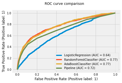
Figure 1: ROC curves

Comparing the indices in Table 2 we conclude that the ML methods perform better that the traditional LR, at least on this database and for single defaults. It is therefore important to compare the discrepancy in joint defaults that they entail.

6.2 Moments and mixing distributions

We provide the estimates of the moments, relevant for the joint defaults and for the number of defaults, and then the parameters of the beta mixing variables.

Table 3 provides the first two empirical moments of $Q_{h}$ and the resulting default correlations, for LR and for each ML model.

Moments	LR	RF	AB	KNN
$p$	0.2635	0.2232	0.2234	0.2209
$\pi_{2}$	0.0883	0.0925	0.0901	0.1023
$\rho$	0.0975	0.2462	0.2319	0.3108

Table 3: Moments estimated with LR and with different ML techniques.

The LR method seems to overestimate the first and underestimate the second order moment, if compared with the ML methods. As a consequence of the relationship among $p$, $\pi_{2}$ and $\rho$, ML techniques are capable to capture higher correlations $\rho$ among default. This preliminary result has to be further investigated to see whether is $p$ or $\rho$ that mainly affects the tail of the loss.

As for the beta mixing variables, using the method of moments, we get the following densities

(a) AB density

(b) LR density

(c) RF density

(d) KNN density

Figure 2: Beta binomial pmf estimated with LR, AB RF and KNN.

Figure 2 shows that the three ML methods provide similar densities, while the LR is significantly different, also in the tails. This will be reflected in the analysis below, particularly in the risk measures.

The corresponding parameters $a,b$ are in Table 4. The remaining entries of the Table are the theoretical or paramerical mean and correlation, which are the counterparts of the emprical - or non parametric - ones in the previous Table:

$\beta$-parameters	LR	RF	AB	KNN
$a$	2.42	0.68	0.73	0.48
$b$	6.78	2.38	2.57	1.72
$p$	0.2630	0.2222	0.2212	0.2182
$\rho$	0.0980	0.2463	0.2326	0.3125

Table 4: Estimated parameters of the beta distribution for each LR/ML model

The Kolmogorov-Smirnov test of the four $\beta$ distributions reject their appropriateness to describe the mixing variable, since the $p$-value is close to zero in all cases. However, Table 4 shows that the theoretical moments are very close to the non parametrical ones. This means that, despite the misspecifications for the distribution of $Q$, we expect theoretical and empirical VaR to be close, with a possible more significant discrepancy in correspondence to $\alpha=0.99$ (see Section 3).

7 VaR bounds and estimates

Risk measurement of the credit losses is done through their VaR and ES, computed along Definition 4.1. Both on a small portfolio ($d=25$) and on the overall portfolio ($d=6000$), we compute the VaR and the corresponding ES bounds and values at the levels of confidence $\alpha=0.9;0.95;0.99$.

7.1 Small portfolio

Table 5 provides the analytical bounds for the VaR, in the class of all credit portfolio with given marginal default probability $p$, for each model specification. The minimum VaR is slightly higher for LR, while all the ML techniques perform similarly. This points to the importance of $p$ in determining the aggregate loss, and is a consequence of the fact that LR overestimates the marginal default probability with respect to ML. It needs to be confirmed for the high dimension portfolio, where the differences can be more evident.

VaR	$\alpha=0.9$	$\alpha=0.95$	$\alpha=0.99$
min LR	5	6	7
max LR	25	25	25
min RF	4	5	6
max RF	25	25	25
min KNN	4	4	5
max KNN	25	25	25
min AB	5	6	6
max AB	25	25	25

Table 5: VaR bounds for a portfolio of $n=25$ obligors, with the $p=$ vaues of Table 4.

We now consider the effect of the second order and higher order moments on joint defaults. The VaRs and ESs computed with the four beta binomial or parametrical models are reported in Table 6 that account only for the first and second moments, because the beta parameters do (see Appendix A). Table 6 also reports the VaR and ES computed with the empirical distribution of $S$, that account for sample higher order moments.

	LR_e	LR_m	RF_e	RF_m	AB_e	AB_m	KNN_e	KNN_m
$\alpha$	VaR	VaR	VaR	VaR	VaR	VaR	VaR	VaR
0.99%	15	17	23	21	22	21	24	23
0.95%	13	14	19	17	18	16	20	18
0.90%	12	12	15	14	15	14	16	15
$\alpha$	ES	ES	ES	ES	ES	ES	ES	ES
0.99%	18.5275	17.5120	23	21.0017	22.0002	21.0017	24	23
0.95%	16.0755	15.5503	19.0084	17.1024	18.0318	16.2864	20.0019	18.0318
0.90%	14.7849	14.7849	15.3527	14.7752	15.3527	14.7752	16.1432	15.3527

Table 6: Non parametrical vs beta-binomial VaRs and ESs of the distribution of number of defaults for a portfolio of $25$ obligors. LR_e; RF_e , AB_e, KNN_e are the non parametrical distributions for each model and LR_m,RF_m, AB_m, KNN_m are the parametrical distributions for each model.

Compare then the VaRs and ESs obtained for the three ML methods with the VaR and ES obtained with LR. The VaRs and ESs obtained with ML techniques are significantly higher than the ones obtained with LR, independently of whether we look at the emprical or theoretical ones. So, when we include correctly the covariates and obligors’ dependencies, as ML by definition does, we do not underestimate risk. This -compared to the bounds- points to the importance of the moments beyond $p$ in determining the aggregate loss. It needs to be confirmed for the high dimension portfolio, where the differences can be more evident.

Comparing the non parametrical vs the beta VaR for each model in Table 6, we obtain the following results. For the LR case the beta VaR is always bigger than the non parametrical one, showing that LR is not capable to capture heavy tails. This is more evident for $\alpha=0.99$, where the importance of the tails of $Q$ is higher. On the contrary, for all the ML techniques the non parametrical VaR is higher than the beta one. This is in line with the ability of these techniques to capture complex dependencies. For all the models the non parametrical and beta VaR are close, something which supports the idea that the estimates of $p$ and $\rho$ are more important than the higher moments. Indeed, only the former determine the beta parameters, while all the moments subsume the non-parametrical specification of a distribution for $Q_{h}$. Similar comments can be made for the ESs in Table 6. This result cannot be confirmed on the high dimension portfolio, since we do not use for it the emprical distribution.

In Table 7 we compare the fit to the non parametrical distribution of $Q_{h}$, $h=$LR, RF, AB, KNN, of the corresponding beta distribution, using the Kullback-Leibler (KL) distance.

	LR	RF	AB	KNN
KL distance	0.0450	0.1153	0.0783	0.1557

Table 7: KL distance for each model.

The conclusion from Table 7 is that the parametrical pmf is closer to the non parametrical one for the AB technique. We therefore focus on AB and the benchmark LR to estimate the VaR and ES for the large portfolio.

7.2 Large portfolio

We now consider a large portfolio, $d=n=6000$, where the differences between LR and ML are more evident than in the small portfolio, as expected.

Table 8 provides the analytical bounds for the VaR, in the class of all credit portfolios with given marginal default probability $p$, estimated respectively with AB and LR. As one can see, since LR overestimates $p$ with respect to $AB$, without specifying the correlation among defaults, the minimum VaR is higher for LR. This confirms what we concluded about $p$ - and the importance not to overestimate it - from a small portfolio.

VaR	$\alpha=0.9$	$\alpha=0.95$	$\alpha=0.99$
min AB	823	1096	1294
max AB	6000	6000	6000
min LR	1091	1384	1573
max LR	6000	6000	6000

Table 8: VaR bounds, for the $p$ values of Table 4.

We now analyse the effect of dependence on the portfolio risk. Our aim is to stress the differences between ML and LR. We compare the portfolio estimated with AB with our benchmark, LR. In Figure 3, the pmf from AB and LR are overlapped to exhibit the differences in the tail distribution.

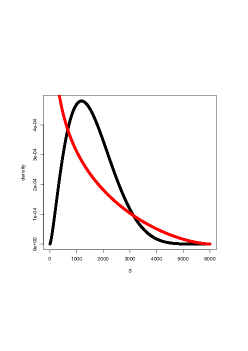
Figure 3: Beta binomial pmf estimated with LR (black) and AB (red).

The theoretical VaRs and ESs obtained from the beta-binomial models corresponding to the parameter $a$ and $b$ estimated using LR and AB and with $d=6000$ are reported in Table 9. Computations are made with the support of $R$.

$\alpha$	VaR LR	VaR AB	ES LR	ES AB
0.99%	3794	4798	4099.6	5131.9
0.95%	3107	3788	3524.3	4395.1
0.90%	2729	3139	3213.0	3916.9

Table 9: Beta-binomial VaR and ES for large portfolios.

Both VaRs and ESs show that using ML to classify individual defaults we have significantly higher measures of risk. The difference between the LR and AB VaRs and $ESs$ in Table 9 is higher for the quantile $\alpha=0.99$. The Table confirms what we concluded about the dependence - and the importance not to underestimate it - from a small portfolio.

We thus have empirical evidence of the importance of ML techniques to properly specify a credit risk model, since they allow us to incorporate the risk coming from dependencies among covariates, that seems to be the more relevant factor affecting the tail of the loss, even without using all moments.

Appendix A Beta and Beta Binomial distributions

Let $Q$ have a Beta distribution of parameters $a$ and $b$, i.e. $Q\sim\beta(a,b)$, its density $g_{Q}$ is given by

$$g_{Q}(q)=\frac{1}{\beta(a,b)}q^{a-1}(1-q)^{b-1},\qquad a,b>0,\quad 0<q<1$$ (A.1)

where

$$\beta(a,b)=\int_{0}^{1}z^{a-1}(1-z)^{b-1}dz,\qquad 0<z<1$$ (A.2)

Standard calculations give:

$$\pi_{k}=\prod_{j=0}^{k-1}\frac{a+j}{a+b+j},$$ (A.3)

in particular

$$\pi=\frac{a}{a+b},\,\,\,\text{and}\,\,\,\rho_{y}=\frac{1}{a+b+1}.$$

A Beta Binomial random variable $S$ with parameters $a,b$ and $d$, $S\sim\beta Bin(a,b,d)$, has pmf $p_{S}(k)$ given by

$$p_{S}(k)=\mathbb{P}(S=k)=\binom{d}{k}\frac{\beta(a+k,b+d-k)}{\beta(a,b)},\,\,\,k\leq d.$$ (A.4)

Appendix B Dataset description

For each client the dataset contains the values of 24 covariates, which include demographic variables, repayment status, past payments, past bill amount, and an indicator of default, namely:

• ID: ID of each client

• LIMIT_BAL: Amount of the given credit (NT dollar), which includes both the individual consumer credit and his/her family (supplementary) credit.

• SEX: Gender (1 = male; 2 = female)

• EDUCATION: (1 = graduate school; 2 = university; 3= high school; 4= others; 5= unknown; 6= unknown)

• MARRIAGE: Marital status (1 = married; 2 = single; 3 = others)

• AGE: Age in years

• PAY_1 to 6 (with 1 missing): Repayment status in September to April 2005 (-1=pay duly, 1=payment delay for one month, 2=payment delay for two months, … 8=payment delay for eight months, 9=payment delay for nine months and above)

• BILL_AMT1 to 6: Amount of bill statement in September to April, 2005 (NT dollar)

• PAY_AMT1: Amount of previous payment in September to April, 2005 (NT dollar)

• default.payment.next.month: Default payment (1=yes, 0=no)

Table 10 provides the descriptive statistics of the data.

-	ID	LIMIT_BAL	SEX	EDUCATION	MARRIAGE	AGE	-
count	30000	30000	30000	30000	30000	30000	-
mean	15000.5	167484.3227	-	-	-	35.4855	-
std	8660.398374	129747.6616	-	-	-	9.217904068	-
min	1	10000	1	0	0	21	-
25%	7500.75	50000	1	1	1	28	-
50%	15000.5	140000	2	2	2	34	-
75%	22500.25	240000	2	2	2	41	-
max	30000	1000000	2	6	3	79	-
-	BILL_AMT1	BILL_AMT2	BILL_AMT3	BILL_AMT4	BILL_AMT5	BILL_AMT6	-
count	30000	30000	30000	30000	30000	30000	-
mean	51223.3309	49179.07517	47013.1548	43262.94897	40311.40097	38871.7604	-
std	73635.86058	71173.76878	69349.38743	64332.85613	60797.15577	59554.10754	-
min	-165580	-69777	-157264	-170000	-81334	-339603	-
25%	3558.75	2984.75	2666.25	2326.75	1763	1256	-
50%	22381.5	21200	20088.5	19052	18104.5	17071	-
75%	67091	64006.25	60164.75	54506	50190.5	49198.25	-
max	964511	983931	1664089	891586	927171	961664	-
-	PAY_1	PAY_2	PAY_3	PAY_4	PAY_5	PAY_6	-
count	30000	30000	30000	30000	30000	30000	-
mean	-	-	-	-	-	-	-
std	-	-	-	-	-	-	-
min	-2	-2	-2	-2	-2	-2	-
25%	-1	-1	-1	-1	-1	-1	-
50%	0	0	0	0	0	0	-
75%	0	0	0	0	0	0	-
max	8	8	8	8	8	8	-
-	PAY_AMT1	PAY_AMT2	PAY_AMT3	PAY_AMT4	PAY_AMT5	PAY_AMT6	def_pay
count	30000	30000	30000	30000	30000	30000	30000
mean	5663.5805	5921.1635	5225.6815	4826.076867	4799.387633	5215.502567	0.2212
std	16563.28035	23040.8704	17606.96147	15666.15974	15278.30568	17777.46578	0.415061806
min	0	0	0	0	0	0	0
25%	1000	833	390	296	252.5	117.75	0
50%	2100	2009	1800	1500	1500	1500	0
75%	5006	5000	4505	4013.25	4031.5	4000	0
max	873552	1684259	896040	621000	426529	528666	1

Table 10: Descriptive statistics.

The correlation matrix of the 24 covariates is presented here as Figure 4.

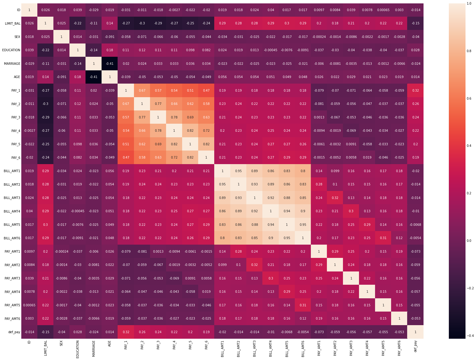
Figure 4: Correlation matrix of the variables.

Figure 5 provides the calibration curves of default probabilities for each ML method.

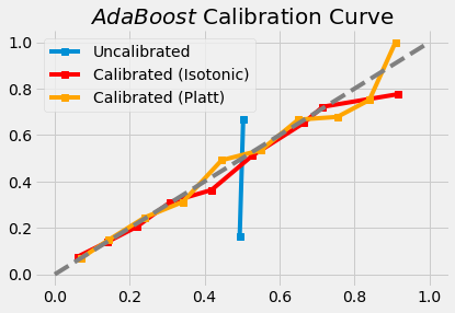
(a) AB curve

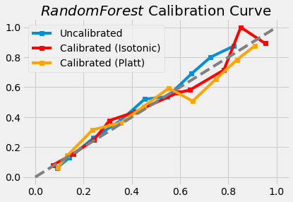
(b) RF curve

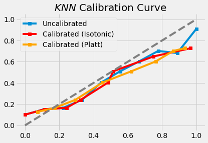
(c) KNN curve

Figure 5: Calibration curves for AB RF and KNN.

References

- Acerbi and Tasche, (2002) Acerbi, C. and Tasche, D. (2002). On the coherence of expected shortfall. Journal of Banking & Finance, 26(7):1487–1503.
- Artzner et al., (1999) Artzner, P., Delbaen, F., Eber, J.-M., and Heath, D. (1999). Coherent measures of risk. Mathematical finance, 9(3):203–228.
- Bartlett and Traskin, (2006) Bartlett, P. and Traskin, M. (2006). Adaboost is consistent. Advances in Neural Information Processing Systems, 19.
- Basoğlu et al., (2018) Basoğlu, I., Hörmann, W., and Sak, H. (2018). Efficient simulations for a bernoulli mixture model of portfolio credit risk. Annals of Operations Research, 260(1):113–128.
- Bellotti and Crook, (2009) Bellotti, T. and Crook, J. (2009). Support vector machines for credit scoring and discovery of significant features. Expert systems with applications, 36(2):3302–3308.
- Chatterjee and Barcun, (1970) Chatterjee, S. and Barcun, S. (1970). A nonparametric approach to credit screening. Journal of the American statistical Association, 65(329):150–154.
- Chen et al., (2021) Chen, S., Guo, Z., and Zhao, X. (2021). Predicting mortgage early delinquency with machine learning methods. European Journal of Operational Research, 290(1):358–372.
- Devroye et al., (1994) Devroye, L., Gyorfi, L., Krzyzak, A., and Lugosi, G. (1994). On the strong universal consistency of nearest neighbor regression function estimates. The Annals of Statistics, 22(3):1371–1385.
- Dumitrescu et al., (2022) Dumitrescu, E., Hue, S., Hurlin, C., and Tokpavi, S. (2022). Machine learning for credit scoring: Improving logistic regression with non-linear decision-tree effects. European Journal of Operational Research, 297(3):1178–1192.
- Fontana et al., (2021) Fontana, R., Luciano, E., and Semeraro, P. (2021). Model risk in credit risk. Mathematical Finance, 31(1):176–202.
- Frey and McNeil, (2001) Frey, R. and McNeil, A. J. (2001). Modelling dependent defaults. Technical report, ETH Zurich.
- Gunnarsson et al., (2021) Gunnarsson, B. R., Vanden Broucke, S., Baesens, B., Óskarsdóttir, M., and Lemahieu, W. (2021). Deep learning for credit scoring: Do or dont́? European Journal of Operational Research, 295(1):292–305.
- Hamori et al., (2018) Hamori, S., Kawai, M., Kume, T., Murakami, Y., and Watanabe, C. (2018). Ensemble learning or deep learning? application to default risk analysis. Journal of Risk and Financial Management, 11(1):12.
- Kenett and Zacks, (2021) Kenett, R. S. and Zacks, S. (2021). Modern industrial statistics: With applications in R, MINITAB, and JMP. John Wiley & Sons.
- Kruppa et al., (2013) Kruppa, J., Schwarz, A., Arminger, G., and Ziegler, A. (2013). Consumer credit risk: Individual probability estimates using machine learning. Expert Systems with Applications, 40(13):5125–5131.
- Lessmann et al., (2015) Lessmann, S., Baesens, B., Seow, H.-V., and Thomas, L. C. (2015). Benchmarking state-of-the-art classification algorithms for credit scoring: An update of research. European Journal of Operational Research, 247(1):124–136.
- Mahbobi et al., (2021) Mahbobi, M., Kimiagari, S., and Vasudevan, M. (2021). Credit risk classification: an integrated predictive accuracy algorithm using artificial and deep neural networks. Annals of Operations Research, pages 1–29.
- McNeil et al., (2005) McNeil, A. J., Frey, R., and Embrechts, P. (2005). Quantitative risk management, volume 3. Princeton university press.
- Sadhwani et al., (2021) Sadhwani, A., Giesecke, K., and Sirignano, J. (2021). Deep learning for mortgage risk. Journal of Financial Econometrics, 19(2):313–368.
- Scornet et al., (2015) Scornet, E., Biau, G., and Vert, J.-P. (2015). Consistency of random forests. The Annals of Statistics, 43(4):1716–1741.
- Tsai et al., (2014) Tsai, C.-F., Hsu, Y.-F., and Yen, D. C. (2014). A comparative study of classifier ensembles for bankruptcy prediction. Applied Soft Computing, 24:977–984.
- Wang et al., (2018) Wang, M., Yu, J., and Ji, Z. (2018). Personal credit risk assessment based on stacking ensemble model. In International Conference on Intelligent Information Processing, pages 328–333. Springer.
- Yeh and Lien, (2009) Yeh, I.-C. and Lien, C.-h. (2009). The comparisons of data mining techniques for the predictive accuracy of probability of default of credit card clients. Expert systems with applications, 36(2):2473–2480.
- Yu et al., (2010) Yu, L., Yue, W., Wang, S., and Lai, K. K. (2010). Support vector machine based multiagent ensemble learning for credit risk evaluation. Expert Systems with Applications, 37(2):1351–1360.