Upper and Lower Bounds for the Correlation Length of the Two-Dimensional Random-Field Ising Model

Abstract.

We study the rate of correlation decay in the two-dimensional random-field Ising model at weak field strength $\varepsilon$. We combine elements of the recent proof of exponential decay of correlations with a quantitative refinement of a result of Aizenman–Burchard on the tortuosity of random curves to obtain an upper bound of the form $\exp(\exp(O(1/\varepsilon^{2})))$ on the correlation length of the model at all temperatures. Conversely, we show, by adapting methods of Fisher–Fröhlich–Spencer, that on square domains of side length as large as $\exp(O(1/\varepsilon^{2/3}))$ the model continues to exhibit strong dependence on boundary conditions at low temperature.

1. Overview

The random-field Ising model (RFIM) is a prime example of a disordered spin system. It is obtained by subjecting the standard Ising model to a random (quenched) external magnetic field composed of independent and identically distributed random variables. The model is described by the formal random Hamiltonian

(1.1) $$H^{h}(\sigma):=-J\sum_{u\sim v}\sigma_{u}\sigma_{v}-\sum_{v}(\eta+\varepsilon h_{v})\sigma_{v},$$

where the Ising spins $\sigma$ take values in $\{-1,1\}$, $J>0$ is the coupling strength, $\varepsilon>0$ is the disorder intensity (or the strength of the random field), $\eta\in\mathbb{R}$ is the intensity of the homogeneous external field and $(h_{v})_{v\in\mathbb{Z}^{2}}$ is the random field, which we take here to consist of independent standard Gaussian random variables. The seminal work of Imry–Ma [17] predicted that the addition of the random field to the two-dimensional Ising model causes the model to lose its ordered low-temperature phase and become disordered at all temperatures (including zero temperature), for every disorder intensity $\varepsilon>0$. This prediction was given a rigorous proof in the celebrated work of Aizenman–Wehr [4, 5]. We discuss here the question of quantifying the rate of correlation decay, as captured by the order parameter

(1.2) $$m(L):=\frac{1}{2}\left(\mathbb{E}\left[\left\langle\sigma_{0}\right\rangle_{\Lambda(L)}^{+}\left(h_{v}\right)\right]-\mathbb{E}\left[\left\langle\sigma_{0}\right\rangle_{\Lambda(L)}^{-}\left(h_{v}\right)\right]\right),$$

where $\left\langle\sigma_{0}\right\rangle_{\Lambda(L)}^{+}\left(h_{v}\right)$ and $\left\langle\sigma_{0}\right\rangle_{\Lambda(L)}^{-}\left(h_{v}\right)$ denote the thermal expectation value of the spin at the origin for the given realization $(h_{v})$ of the random field, when the model is sampled in the discrete square $\Lambda(L):=\{-L,\ldots,L\}^{2}$ with $+$ or $-$ boundary conditions, respectively, and where the operator $\mathbb{E}$ denotes expectation over the values of the random field $(h_{v})$. The order parameter controls several related notions of correlation decay, as discussed in [3, Section 1.2].

It is generally expected that at high enough disorder, be it thermal or due to noisy environment, correlations decay exponentially fast. Results in this vein for systems related to the RFIM can be found in the works of Berretti [6], Imbrie–Fröhlich [15] and Camia–Jiang–Newman [9]. The main challenge thus lies in analyzing the behavior at low temperature and weak disorder strength. In recent years there has been major progress in quantifying the rate of correlation decay for the two-dimensional RFIM in the latter regime. Upper bounds were established in a series of works [10, 3, 2, 13, 12] which culminated in a proof of exponential decay of correlations at all temperatures and all positive disorder strengths. Precisely, the following theorem was proved.

Theorem (exponential decay of correlations [12, 2]).

In the nearest-neighbor random-field Ising model on $\mathbb{Z}^{2}$, as specified by (1.1), at any coupling strength $J>0$ and disorder intensity $\varepsilon>0$ there exist constants $C(J/\varepsilon),c(J/\varepsilon)>0$, depending only on the ratio $J/\varepsilon$, such that at all temperatures $T\geq 0$ and homogeneous external field $\eta\in\mathbb{R}$ the order parameter satisfies for all integer $L\geq 1$,

(1.3) $$m(L)\leq C(J/\varepsilon)\exp(-c(J/\varepsilon)L).$$

While the theorem establishes exponential decay of correlations, it leaves open the question of how the correlation length varies as the ratio $J/\varepsilon$ tends to infinity (at low temperature). Here, the notion of “correlation length” can be given several interpretations: One standard definition is the infimum over $\zeta$ for which $m(L)\leq e^{-L/\zeta}$ for all sufficiently large $L$; denote this value by $\zeta_{1}=\zeta_{1}(T,J,\eta,\varepsilon)$. A second possibility is the minimal value of $L$ for which $m(L)$ drops below some fixed threshold $m$ (e.g., $m=1/2$); denote this value by $\zeta_{2}:=\zeta_{2}(T,J,\eta,\varepsilon,m)$. In [2] it was asked to determine the order of magnitude of the correlation length. It was noted that $\zeta_{2}\leq\exp\left(\exp\left(O\left((\frac{J}{\varepsilon})^{2}\right)\right)\right)$ was established in [3] (for each fixed $T,\eta$ and $m$) and that the behavior $\zeta_{1}=\exp(O((J/\varepsilon)^{2}))$ was discussed in [7].

The goal of this work is to provide upper and lower bounds on the correlation length of the two-dimensional Ising model. The following is our main result.

Theorem 1.

Consider the nearest-neighbor random-field Ising model on $\mathbb{Z}^{2}$, as specified by (1.1), at coupling strength $J>0$ and disorder intensity $\varepsilon>0$ satisfying that $\frac{J}{\varepsilon}\geq 1$.

1. There exists a universal constant $C>0$ such that at all temperatures $T\geq 0$ and homogeneous external field $\eta\in\mathbb{R}$, the correlation length $\zeta_{1}$ satisfies

   (1.4) $$\zeta_{1}(T,J,\eta,\varepsilon)\leq\exp\left(\exp\left(C\left(\frac{J}{\varepsilon}\right)^{2}\right)\right).$$

2. For each $0<\delta<1$ there exists $c(\delta)>0$ (depending only on $\delta$) such that at zero temperature and zero homogeneous external field the correlation length $\zeta_{2}$ satisfies

   (1.5) $$\zeta_{2}(0,J,0,\varepsilon,1-\delta)\geq\exp\left(c(\delta)\left(\frac{J}{\varepsilon}\right)^{2/3}\right).$$

   In other words, when $L<\exp\left(c(\delta)(\frac{J}{\varepsilon})^{2/3}\right)$ the spin at the origin of the ground state in $\Lambda(L)$ with $+$ boundary conditions is equal to $1$ with probability (over the random field) greater than $1-\frac{1}{2}\delta$.

Our approach to the correlation length upper bound (1.4) builds upon the recent proofs of exponential decay of correlations [12, 2]. While the available proofs do not provide an explicit upper bound on the correlation length, it was noted in [2] that such a bound will follow from a quantitative refinement of one of the main tools of the proof, the Aizenman–Burchard theorem on the tortuosity of random curves [1]. In Section 2 we provide such a refinement, which is then used in Section 3 to derive the upper bound (1.4). Our quantitative refinement of the Aizenman–Burchard theorem, given in Theorem 10, may be of use in other contexts as well.

Section 4 and Appendix A are devoted to the proof of the lower bound (1.5), derived in a somewhat more general setting. The proof adapts to the two-dimensional setting the “coarse graining” methods of Fisher–Fröhlich–Spencer [14] which were developed in their discussion of the phase transition that the three-dimensional RFIM displays at low temperature as the random-field strength is varied (the transition was given rigorous proofs in the celebrated works of Imbrie [16] and Bricmont–Kupiainen [8]). This approach will in fact give us a stronger result, which is that below the lower bound we should expect all spins in $\Lambda(L)$, not just at the origin, to be equal to 1 with high probability.

While this work was in progress, a sharper estimate of the correlation length $\zeta_{2}$ was established by Ding–Wirth [11]. For $\frac{J}{\varepsilon}\geq 1$ and $0<\delta<1$, they proved the lower bound $\zeta_{2}(0,J,0,\varepsilon,\delta)\geq\exp\left(c(\delta)(\frac{J}{\varepsilon})^{4/3}\frac{1}{\log(J/\varepsilon)}\right)$ at zero temperature and the near-matching upper bound $\zeta_{2}(T,J,0,\varepsilon,\delta)\leq\exp\left(C(\delta)(\frac{J}{\varepsilon})^{4/3}\right)$ at all temperatures $T\geq 0$.

2. The Aizenman–Burchard Theorem and a Quantitative Refinement

2.1. A Brief Introduction

In this section we present a quantitative refinement to a result by Aizenman and Burchard regarding fractality of random curves in $\mathbb{R}^{d}$ [1].

A system of random curves is a collection of set-valued random variables, $(\mathcal{F}_{\delta})_{\delta>0}$, where each element of $\mathcal{F}_{\delta}$ is some piecewise linear curve, composed of line segments of length $\delta$. In essence, Aizenman and Burchard showed that if a system of random curves satisfies an assumption, which we will call H2, then as $\delta$ gets lower, $\mathcal{F}_{\delta}$ will resemble a collection of curves of Hausdorff dimension greater than some constant $d_{\min}>1$ independent of $\delta$. Our goal in this section is to quantify both $d_{\min}$ and also the rate at which $\mathcal{F}_{\delta}$ starts to resemble such a collection of curves.

The assumption H2 depends on three parameters, $0<\rho<1,\sigma>0$, and $K>0$, and it goes roughly as follows; for any set of $n$ cylinders in $\mathbb{R}^{d}$ with aspect ratio $\sigma$ and length greater than $\delta$, the probability that each of the cylinders is crossed by some curve in $\mathcal{F}_{\delta}$ is less than $K\rho^{n}$. Our improvement to the Aizenman–Burchard theorem will be to quantify the fractality of a system of curves $(\mathcal{F}_{\delta})_{\delta>0}$ satisfying H2 in terms of the parameter $\rho$ when it’s close to 1. More specifically, assuming $\rho=1-\varepsilon$ for small enough $\varepsilon>0$, we will show the lower bound

$$d_{\min}\geq 1+\kappa\frac{\varepsilon^{2}}{\log\left(1/\varepsilon\right)^{3}},$$

for a universal constant $\kappa$ independent of $\rho$.

This quantification, in addition to a more technical one we will define later, will be crucial later in this paper for obtaining the upper bound (1.4).

2.2. Definitions

Definition 2.

A finite collection of subsets in $\mathbb{R}^{d}$ is called well separated if for any two sets $A,B$ in it:

$$d(A,B)\geq\max(\text{diam}(A),\text{diam}(B)),$$

where $d(A,B):=\inf\{d(x,y)\,|\,x\in A,\,y\in B\}$, $d(x,y)$ is the Euclidean distance between $x,y\in\mathbb{R}^{d}$, and where $\text{diam}(A):=\sup\{d(x,y)\,|\,x,y\in A\}$ is the Euclidean diameter of $A$.

Definition 3.

A $\delta$-polygonal path in $\mathbb{R}^{d}$ is a piece-wise linear continuous path, $\gamma:I\rightarrow\mathbb{R}^{d}$ (where $I\subseteq\mathbb{R}$ is some closed interval), formed by the concatenation of finitely many segments of length $\delta$.

Definition 4.

A system of random curves with short variable cutoff in a compact set $\Lambda\subseteq\mathbb{R}^{d}$ is a collection of set-valued random variables $\mathcal{F}=\left(\mathcal{F_{\delta}}\right)_{0<\delta\leq 1}$, with each $\mathcal{\mathcal{F}_{\delta}}$ equaling a random finite set of $\delta$-polygonal paths. Such collections form closed sets in the Hausdorff metric contained in $\Lambda$ and the sigma algebra in this case is the one induced by the Hausdorff metric. We will usually denote the probability measure of the space on which $\mathcal{F_{\delta}}$ is defined by $\mathbb{P}_{\delta}$.

In a way, a system of random curves with short variable cutoff is a substitute for sampling a random continuous curve (or collection of curves) via discrete approximations. We sample random piece-wise linear curves with step length $\delta$, and the smaller $\delta$ gets the more complex our curves become.

Definition 5.

A system of random curves with short variable cutoff $\mathcal{F}=\left(\mathcal{F_{\delta}}\right)_{0<\delta\leq 1}$ in some compact $\Lambda\subseteq\mathbb{R}^{d}$ is said to satisfy hypothesis H2 with parameters $0<\rho<1$ and$\,\sigma\geq 1$, if there exists a constant $C>0$ such that for any $\delta>0$ and any finite collection of well-separated cylinders $(A_{i})_{i=1}^{m}\subseteq\Lambda$ with aspect ratio $\sigma$ and lengths $>\delta$ it holds that

(2.1) $$\mathbb{P}_{\delta}\left(\textup{$\bigcap_{i=1}^{m}\{$$A_{i}$ is crossed in the long direction by a curve in $\mathcal{F}_{\delta}$\}}\right)\leq C\rho^{m},$$

and the constant $C$ is independent of $m$ and the chosen cylinders. Here the length of the cylinder is the length between its two circular bases, and the aspect ratio $\sigma$ is the ratio between its length and the radius of the bases. By a crossing of a cylinder we mean a path contained in the cylinder which connects its two bases. Note that the bases need not be parallel to one of the coordinate hyper-planes $\{x_{i}=0\}$.

Remark 6.

In the original theorem [1], the assumption that $\sigma\geq 1$ is ommited and in its place a crossing of the cylinder is defined as a crossing of its long side rather than a crossing from one base to the other. Here we will simplify things by just looking at the $\sigma\geq 1$ and only at crossings from one base to the other. As will be seen later, our proof will also work if the assumption of $\sigma\geq 1$ is replaced by $\sigma\geq\sigma_{0}$ for some $\sigma_{0}>0$.

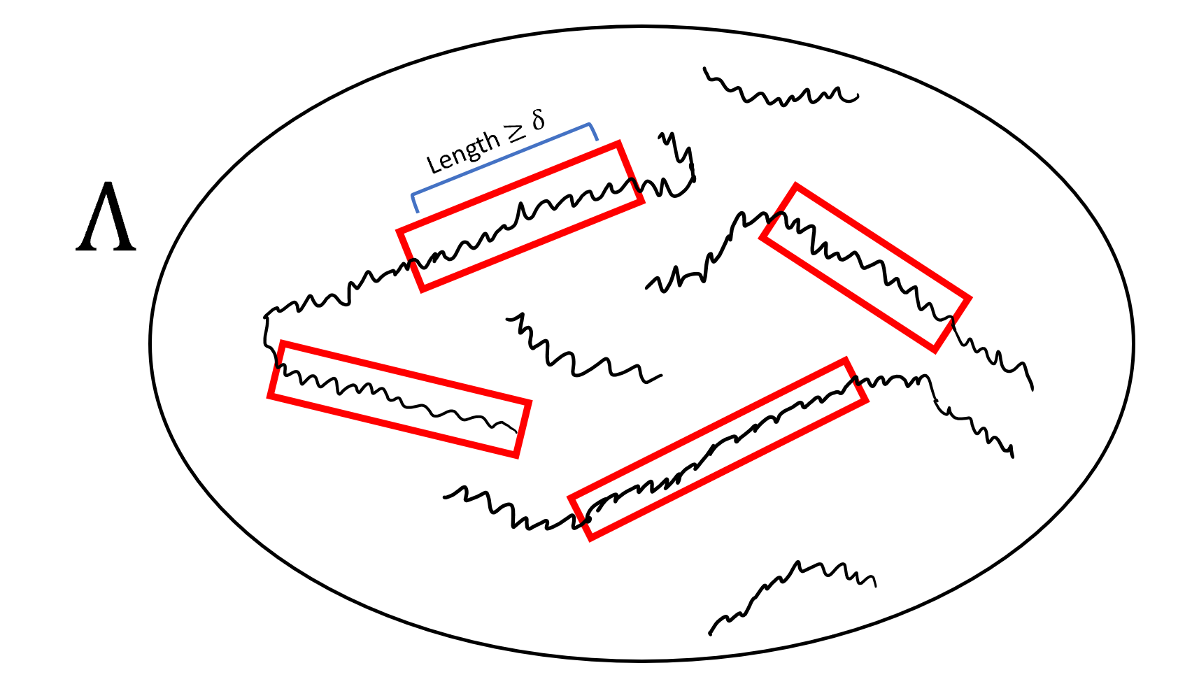
Figure 2.1. In order for hypothesis H2 to hold, we need that for every collection of cylinders (with sufficient length and separation) the probability of all of them being crossed by curves in $\mathcal{F_{\delta}}$ is exponentially decreasing with the number of cylinders.

Definition 7.

For a set $A\subseteq\mathbb{R}^{d}$, parameters $\ell>0$ and $s$, we define the $s,\ell$ capacity of $A$ to be:

(2.2) $$\frac{1}{\text{Cap}_{s;\ell}(A)}=\inf_{\mu\geq 0,\mu(A)=1}\iint_{A\times A}\frac{\mu(dx)\mu(dy)}{\max(\left|x-y\right|,\ell)^{s}},$$

where the infimum is over all probability measures on $A$.

The following properties of the capacity from [1] will be of use to us:

Claim 8.

Let $A\subset\mathbb{R}^{d}$. Then:

(i) For any covering of $A$ by sets $(B_{j})$ of diameter at least $\ell$:

(2.3) $$\sum_{j}\text{diam}(B_{j})^{s}\geq\text{Cap}_{s;\ell}(A).$$

(ii) The minimal number of elements in a covering of $A$ by sets of diameter $\ell$, $\mathcal{N}(A,\ell)$, satisfies:

(2.4) $$\mathcal{N}(A,\ell)\geq\text{Cap}_{s;\ell}(A)\cdot\ell^{-s}.$$

(iii) If $\inf_{\ell>0}\text{Cap}_{s;\ell}(A)>0$, then the Hausdorff dimension of $A$ is at least $s$.

2.3. The Main Theorem

Aizenman and Burchard proved the following theorem relating the hypothesis H2 and the capacity (and thus Hausdorff dimension and tortuosity) of a random curve system:

Theorem 9.

Let $\mathcal{F}=(\mathcal{F_{\delta}})_{0<\delta\leq 1}$ be a system of random curves with short variable cutoff in $\Lambda\subseteq\mathbb{R}^{d}$ satisfying hypothesis H2, then there exists some $d_{\min}>1$ such that for any fixed $r>0$ and $s>d_{\min}$, the random variables:

(2.5) $$T_{s,r;\delta}:=\inf_{\mathcal{C}\in\mathcal{F}_{\delta},\text{diam}(C)\geq r}\text{Cap}_{s;\delta}(\mathcal{C})$$

satisfy that for every $\varepsilon>0$ there exists a $\mu>0$ such that for all $\delta$:

$$\mathbb{P}(T_{s,r;\delta}\leq\mu)<\varepsilon.$$

As stated before, the intuition of the theorem is that as we take $\delta$ to be smaller and smaller, the random curves will resemble a set of Hausdorff dimension $>d_{min}$ more and more. This intuition can be formalized in terms of a scaling limit as in [1], however we will not use nor need it here. Our goal in this section will be to give an improvement of the result, by giving quantitative bounds for the minimal dimension $d_{min}$ and in addition probabilistic bounds on how the random variables $T_{s,r;\delta}$ are bounded away from zero. Both of these will be given in terms of the parameter $\rho$ from hypothesis H2. We shall prove the following:

Theorem 10.

Let $\mathcal{F}=(\mathcal{\mathcal{F}_{\delta}})_{0<\delta\leq 1}$ be a system of random curves in a compact subset $\Lambda\subset\mathbb{R}^{d}$ with a short variable cutoff. Suppose $\mathcal{F}$ satisfies hypothesis H2 with parameters $\rho=1-\varepsilon$, where $0<\varepsilon<\frac{1}{10}$, and $\sigma>0$. Then there exists some constant $\alpha$ satisfying

(2.6) $$\alpha\geq\kappa\frac{\varepsilon^{2}}{\log\left(1/\varepsilon\right)^{3}},$$

so that for all $\delta>0$ and for all $\mu>0$

(2.7) $$\mathbb{P}_{\delta}(T_{1+\alpha,1;\delta}<\mu)\leq\mu^{\frac{K}{\log(1/\varepsilon)}},$$

with $\kappa,K>0$ depending only on $\sigma$ and $\Lambda$.

2.4. Straight Runs

Policy regarding constants: During proofs in this section, we will use $K$ (or $C$) and $\kappa$ (or $c$) to denote universal constants depending only on $\sigma$ and $\Lambda$, which may increase or decrease respectively from line to line.

Our goal in this section will be to give a lower bound for the capacity in terms of a function on a random variable, $k_{0;s}$.

Definition 11.

Let $\gamma>1$ be some constant (called the “scaling factor”), $\mathcal{C}$ a curve in $\mathbb{R}^{d}$. A $\gamma$-straight run at scale $L$ for $\mathcal{C}$ is a crossing of $\mathcal{C}$ from one spherical “face” to the other of some cylinder of length $L$ and radius $\frac{9}{2\sqrt{\gamma}}L$. We say a straight run is nested in another straight run if the cylinder of the first is contained in the cylinder of the second one.

Definition 12.

For a curve $\mathcal{C}$ in $\mathbb{R}^{d}$, positive integer $k_{0}$, scaling factor $\gamma>1$, and length $\ell>0$, we say straight runs in $\mathcal{C}$ are $(\gamma,k_{0})$-sparse down to length $\ell>0$, if for any $n\geq\frac{1}{2}k_{0}$ and positive integers $1\leq k_{1}<k_{2}<...<k_{n}\leq 2n$, $\gamma^{-k_{n}}\geq\ell$, there is no nested sequence of $\gamma$-straight runs at scales $\gamma^{-k_{1}},\gamma^{-k_{2}},...,\gamma^{-k_{n}}$.

Aizenman and Burchard proved the following theorem relating straight runs and their sparsity to the Hausdorff dimension ([1], Theorem 5.1)

Theorem 13.

Let $\gamma>1$ be a scaling factor and let $m=\left\lfloor\gamma\right\rfloor$. If in some curve $\mathcal{C}$ in $\mathbb{R}^{d}$ straight runs are $(\gamma,k_{0})$-sparse (down to all scales), then:

(2.8) $$\dim_{\mathcal{H}}(\mathcal{C})\geq\frac{\log\left(m(m+1)\right)}{2\log(\gamma)},$$

where $\dim_{\mathcal{H}}(\mathcal{C})$ denotes the Hausdorff dimension of $\mathcal{C}$.

Unfortunately for us, this theorem is only of use in a scaling limit setting, not the piece-wise linear curves we are interested in. Luckily though, the above theorem is actually implied from a more general fact, also proven in [1] (Lemma 5.2 and Lemma 5.4, equation (5.22)).

Lemma 14.

Let $\mathcal{C}$ be a curve in $\mathbb{R}^{d}$ in which straight runs are $(\gamma,k_{0})$-sparse down to scale $\ell$. Then:

(2.9) $$\text{Cap}_{s;\ell}(\mathcal{C})\geq\left(\left(\frac{\gamma}{m}-1\right)\cdot\text{diam}(\mathcal{C})\right)^{s}\left(\gamma^{s\cdot k_{0}}+\frac{\beta}{1-\gamma^{s}/\beta}\right)^{-1},$$

where $m$ is any integer in $[\gamma/2,\gamma]$, $\beta=\sqrt{m(m+1)}$, and $\gamma^{s}<\beta$.

Note that what matters to us most is the smallest $k_{0}$ for which straight runs are $(\gamma,k_{0})$-sparse. Our goal in this section will be to prove a relation between hypothesis H2 and the distribution of this smallest $k_{0}$.

Lemma 15.

Let $\mathcal{F}=(\mathcal{\mathcal{F}_{\delta}})_{0<\delta\leq 1}$ be a system of random curves with short variable cutoff in $\Lambda\subseteq\mathbb{R}^{d}$ satisfying hypothesis H2 with parameters $\rho=1-\varepsilon,\sigma$. Suppose $\gamma>\max(4d,\sigma^{2})$. Then for small enough $\varepsilon$ there exists constants $K_{0},K_{1}>0$ depending only on $\sigma$ and $\Lambda$ for which:

(2.10) $$\mathbb{P}_{\delta}\left(\begin{array}[]{c}\textup{in some curve in $\mathcal{F}_{\delta},$ there is a nested sequence of straight runs}\\ \textup{at scales }\gamma^{-k_{1}},\gamma^{-k_{2}},...,\gamma^{-k_{n}}\end{array}\right)$$

$$\leq K_{1}\gamma^{2dk_{n}}e^{K_{1}n-K_{0}\sqrt{\gamma}\varepsilon n},$$

for any increasing sequence of positive integers $k_{1},\ldots,k_{n}$ such that $\gamma^{-k_{n}}\geq\delta$.

Proof.

First note that if a curve in $\mathbb{R}^{d}$ crosses a cylinder of length $L$ and radius $\frac{9}{2\sqrt{\gamma}}L$, then it also crosses a cylinder of radius $\frac{5}{\sqrt{\gamma}}L$ and length $\frac{L}{2}$, which is centered on a line between two points in the discrete lattice $\frac{L}{\gamma}\mathbb{Z}^{d}$. Therefore, we can instead bound the probability of there existing a sequence of straight runs whose cylinders are centered on a segment in $\gamma^{-k_{1}-1}\mathbb{Z}^{d},\ldots,\gamma^{-k_{n}-1}\mathbb{Z}^{d}$.

The number of possible positions for the cylinder at scale $\gamma^{-k_{1}}$ will be at most $K_{\Lambda}\gamma^{2dk_{1}}$, where $K_{\Lambda}\approx\textup{Vol}(\Lambda)$ is a constant only depending on $\Lambda$. Then the number of possible positions for the second cylinder at scale $\gamma^{-k_{2}}$ will be at most $K_{d}\gamma^{2d(k_{2}-k_{1})}$ for a constant $K_{d}$ depending only on the dimension. Indeed, to pick the second cylinder given the first cylinder we need to pick two points in the lattice $\gamma^{-k_{2}-1}\mathbb{Z}^{d}$ contained in a subset of $\mathbb{R}^{d}$ with volume $K_{d}\gamma^{dk_{1}}$ for appropriate constants depending solely on the dimension. Repeating this until $k_{n}$, we get that the number of possible cylinders at scales $\gamma^{-k_{1}},\gamma^{-k_{2}},...,\gamma^{-k_{n}}$ is bounded above by:

(2.11) $$K_{\Lambda}\gamma^{2dk_{1}}K_{d}\gamma^{2d(k_{2}-k_{1})}\cdots K_{d}\gamma^{2d(k_{n}-k_{n-1})}=K_{d}^{n}\gamma^{2dk_{n}}.$$

For a fixed collection of cylinders $A_{1},..,A_{n}$, with radius and length as above, we want to bound the probability of all of them being crossed at once. This will be done using the assumption regarding hypothesis H2. To match the aspect ratio $\sigma$ in H2, cut each cylinder $A_{i}$ into $\sqrt{\gamma}/10\sigma$ smaller cylinders of aspect ratio $\sigma$ (whose spherical bases are translates of the bases of $A_{i}$). If the length of the original cylinder $A_{i}$ is $L/2$, as described above its radius will be $\frac{5}{\sqrt{\gamma}}L$. Therefore the length of each cylinder obtained from the cutting is $\frac{5L}{\sqrt{\gamma}/\sigma}$ and so each has diameter (diameter as defined in 2, not diameter of the base of the cylinder) of $L\sqrt{\frac{10^{2}}{\gamma}+\frac{(5\sigma)^{2}}{\gamma}}=5L\sqrt{\frac{4+\sigma^{2}}{\gamma}}$. To obtain a collection of well seperated cylinders from the ones cut from $A_{i}$, we pick every second cylinder (since $\sigma\geq 1$), which yields at least $\sqrt{\gamma}/20\sigma$ cylinders.

Finally, note that each section of $A_{i+1}$ intersects at most two of the smaller cylinders $A_{i}$ was cut into, so by removing those two cylinders from each layer $A_{i}$ we get a well seperated collection with at least $n(\sqrt{\gamma}/20\sigma-2)$. Therefore, using hypothesis H2:

(2.12) $$\mathbb{P}_{\delta}(\textup{All the cylinders $A_{1},..,A_{n}$ are crossed)$\leq C(1-\varepsilon)^{n(\sqrt{\gamma}/20\sigma-2)}\leq Ce^{C\sqrt{\gamma}\log(1-\varepsilon)n}\leq Ce^{-K_{0}\sqrt{\gamma}\varepsilon n}$.}$$

Finally, combining (2.11) and (2.12) and applying a union bound, we get our desired result. $\blacksquare$

Remark 16.

This is the only place where the assumption $\sigma\geq 1$ was needed. Were we to replace this assumption with $\sigma\geq\sigma_{0}$ instead, we would have had to pick instead every $\left\lceil\frac{4+\sigma_{0}^{2}}{\sigma_{0}}\right\rceil$-th layer instead. This wouldv’e yielded a similar result, but with the constants depending on $\sigma_{0}$.

Proposition 17.

Let $\mathcal{F}=(\mathcal{F}_{\delta})_{0<\delta\leq 1}$ be a system of random curves with short variable cutoff in $\Lambda\subseteq\mathbb{R}^{d}$ satisfying hypothesis H2 with parameters $\rho,\sigma$. Let $\gamma>\max(4d,\sigma^{2})$ be a scaling factor satisfying the inequality $\gamma^{4d}e^{K_{1}-K_{0}\varepsilon\sqrt{\gamma}}<\frac{1}{8}$, with $K_{0},K_{1}$ being the constants from the above lemma. Then there exist constants $C,c>0$, depending only on $\sigma$ and $\Lambda$, such that for all integer $k_{0}$,

$$\mathbb{P}_{\delta}(\textup{straight runs are }(\gamma,k_{0})\textup{-sparse down to scale $\delta$ for all curves in $\mathcal{F}_{\delta}$)}\geq 1-Ce^{-ck_{0}}.$$

Proof.

Combining Lemma 15 and the definition of sparsity of straight runs, we see that:

(2.13) $$\mathbb{P}_{\delta}(\textup{straight runs are not }(\gamma,k_{0})\textup{-sparse down to scale $\delta$)}\\ \leq\sum_{n=\lceil k_{0}/2\rceil}^{\infty}\sum_{1\leq k_{1}<\cdots<k_{n}\leq 2n,\,\gamma^{-k_{n}}\geq\delta}\mathbb{P}_{\delta}\left(\textup{$\begin{array}[]{c}\textup{there is a nested sequence of straight runs}\\ \textup{at scales}\gamma^{-k_{1}},\gamma^{-k_{2}},...,\gamma^{-k_{n}}\end{array}$}\right)\\ \leq\sum_{n=\lceil k_{0}/2\rceil}^{\infty}\sum_{1\leq k_{1}<\cdots<k_{n}\leq 2n}K_{1}\gamma^{4dn}e^{K_{1}n-K_{0}\sqrt{\gamma}\varepsilon n}\\ \leq K\sum_{n=\lceil k_{0}/2\rceil}^{\infty}{2n\choose n}\gamma^{4dn}e^{K_{1}n-K_{0}\sqrt{\gamma}\varepsilon n}\\ \leq K\sum_{n=\lceil k_{0}/2\rceil}^{\infty}{2n\choose n}\left(\frac{1}{8}\right)^{n}\leq K\sum_{n=\lceil k_{0}/2\rceil}^{\infty}4^{n}\left(\frac{1}{8}\right)^{n}\leq Ce^{-ck_{0}},$$

which is our desired result. $\blacksquare$

We summarize the results of this section in the following proposition:

Proposition 18.

In a system satisfying the conditions of Theorem 10,there exists a random variable $k_{0;\delta}$ such that for any single curve $\mathcal{C}\in\mathcal{F}_{\delta}$:

(2.14) $$\text{Cap}_{s;\delta}(\mathcal{C})\geq\left(\left(\frac{\gamma}{m}-1\right)\cdot\text{diam}(\mathcal{C})\right)^{s}\left(\gamma^{s\cdot k_{0;\delta}}+\frac{\beta}{1-\gamma^{s}/\beta}\right)^{-1},$$

where $k_{0;\delta}=\min(k_{0}\geq 0\textup{ : straight runs are $k_{0;\delta}$ sparse down to scale $\delta$)}$ is a random variable which satisfies:

(2.15) $$\mathbb{P}_{\delta}(k_{0;\delta}>N)\leq Ce^{-cN},N\in\mathbb{N},$$

$\gamma>\max(4d,\sigma^{2})$ is a scaling factor such that $\gamma^{4d}e^{K_{1}-K_{0}\varepsilon\sqrt{\gamma}}<\frac{1}{8}$, $m$ is an integer in $[\gamma/2,\gamma]$, $\beta=\sqrt{m(m+1)}$, and $\gamma^{s}<\beta$.

Before moving on, note that we can simplify the required inequality on $\gamma$ and rewrite it instead as:

(2.16) $$\gamma>K\varepsilon^{-2}\log^{2}\left(\varepsilon\right)=:\gamma_{0}$$

where $K$ is a constant independent of $\rho$ (but depending on the dimension and $\sigma$), and recalling that $\rho=1-\varepsilon$, where $0<\varepsilon<\frac{1}{10}$.

2.5. Completing the Argument

Proof of Theorem 10: Pick a value $\gamma\in(\gamma_{0},2\gamma_{0})$ as in (2.16), with the additional property that $\gamma-\frac{1}{4}$ is an integer. Denote $m=\left\lfloor\gamma\right\rfloor=\gamma-\frac{1}{4}$, $\beta=\sqrt{m(m+1)}$ as before and take $s$ for which

(2.17) $$\gamma^{s}=m\left(1+\frac{1}{m}\right)^{3/8}\leq m\left(1+\frac{1}{m}\right)^{1/2}=\beta.$$

Then by Proposition 18, for any curve $\mathcal{C}$ in $\mathcal{F_{\delta}}$ such that $\text{diam}(\mathcal{C})\geq 1$:

(2.18) $$\text{Cap}_{s;\delta}(\mathcal{C})\geq(\frac{\gamma}{m}-1)^{s}\left(\gamma^{s\cdot k_{0;\delta}}+\frac{\beta}{1-\gamma^{s}/\beta}\right)^{-1}=\frac{1}{4m}\left(\gamma^{s\cdot k_{0;\delta}}+\frac{\beta}{1-\gamma^{s}/\beta}\right)^{-1}.$$

Additionally, the value of $s$ we chose also has the property that:

(2.19) $$\frac{\gamma^{s}}{\beta}=\left(1+\frac{1}{m}\right)^{-1/8}=\left(\frac{m}{\beta}\right)^{1/4},$$

so by (2.14) and (2.15) we get for this value of $s$ and any $\mu>0$ small enough:

(2.20) $$\mathbb{P}(T_{s,1;\delta}<\mu)\leq\mathbb{P}\left(\frac{1}{4m}\left(\gamma^{s\cdot k_{0;\delta}}+\frac{\beta}{1-\gamma^{s}/\beta}\right)^{-1}<\mu\right)=\\ =\mathbb{P}\left(\gamma^{s\cdot k_{0;\delta}}+\frac{\beta}{1-\gamma^{s}/\beta}>\frac{1}{4\mu m}\right)\leq\mathbb{P}\left(\gamma^{s\cdot k_{0;\delta}}+\frac{\beta}{1-(m/\beta)^{1/4}}>\frac{1}{4\mu\beta}\right)=\\ =\mathbb{P}\left(\gamma^{s\cdot k_{0;\delta}}+\frac{\beta^{5/4}}{\beta^{1/4}-m^{1/4}}>\frac{1}{4\beta\mu}\right)\leq\mathbb{P}\left(\gamma^{s\cdot k_{0;\delta}}+4\beta^{5/4}>\frac{1}{4\beta\mu}\right)=\\ =\mathbb{P}\left(k_{0;\delta}>\frac{\log\left(\frac{1}{4\mu\beta}-4\beta^{5/4}\right)}{s\log(\gamma)}\right)\leq\exp\left(-c\frac{\log\left(\frac{1}{4\beta\mu}-4\beta^{5/4}\right)}{s\log(\gamma)}\right)\leq K(\beta\mu)^{\frac{K}{s\log(\gamma)}}\leq K\mu^{\frac{K}{s\log(\gamma)}},$$

and in addition, for $\mu<1$:

(2.21) $$K\mu^{\frac{K}{s\log(\gamma)}}=K\mu^{\frac{K}{\log(\gamma^{s})}}\leq K\mu^{\frac{K}{\log(\beta)}}\leq K\mu^{\frac{K}{\log(\gamma)}}\leq K\mu^{\frac{K}{\log(1/\varepsilon)}},$$

proving (2.7). Finally, in order to get (2.6) we see that:

(2.22) $$s=\frac{\log\left(m\left(1+\frac{1}{m}\right)^{3/8}\right)}{\log(\gamma)}=\frac{\log\left(m\left(1+\frac{1}{m}\right)^{3/8}\right)}{\log(m+1/4)}=\\ \frac{\log\left(m\left(1+\frac{1}{m}\right)^{3/8}\right)}{\log\left(m(1+\frac{1}{4m})\right)}\geq\frac{\log\left(m(1+\frac{1}{m})^{3/8}\right)}{\log\left(m(1+\frac{1}{m})^{1/4}\right)}\geq 1+\frac{1}{8}\frac{\log\left(1+\frac{1}{m}\right)}{\log\left(m(1+\frac{1}{m})^{1/4}\right)}\geq\\ \geq 1+\frac{1}{16m\log(m)}\geq 1+\frac{c}{\gamma\log(\gamma)}\geq 1+c\frac{\varepsilon^{2}}{\ln(1/\varepsilon)^{3}}$$

Therefore, for $\alpha\geq c\frac{\varepsilon^{2}}{\log(1/\varepsilon)^{3}}$ . In the same way, we also get an upper bound on $\alpha$. $\blacksquare$

3. Upper Bound in the Random-Field Ising Model

3.1. Overview of the proof

Our goal in this section will be to prove the first part of Theorem 1. Namely:

Theorem 19.

In the two-dimensional random-field Ising model, for each fixed temperature $T\geq 0$ and external field $\eta\in\mathbb{R}$, the correlation length satisfies

(3.1) $$\zeta_{1}\leq\exp\left(\exp\left(O\left(\frac{J}{\varepsilon}\right)^{2}\right)\right),$$

as $J/\varepsilon$ tends to infinity.

Throughout this section, we fix the temperature $T\geq 0$ and external field $\eta\in\mathbb{R}$ and omit them from the notation.

The Aizenman–Harel–Peled [2] argument relies on analyzing a disagreement percolation; see Section 3 there. At zero temperature, the disagreement percolation is a random set of vertices obtained as follows: one samples two independent instances of the Ising model in $\Lambda(L)$ with the same realization of the random field, one instance with $+$ boundary conditions and the other with – boundary conditions, and sets the disagreement vertices to be those vertices where the two instances differ (at such vertices the instance with $+$ boundary conditions lies strictly above the instance with $-$ boundary conditions, as the temperature is zero). At positive temperature, a more complicated construction is used and the resulting disagreement percolation is a random set consisting of both vertices and edges.

The main result proved for the disagreement percolation is stated in the following lemma taken from [2, Lemma 5.1], which makes use of the Aizenman–Burchard theorem. The zero-temperature version of the lemma was first proved by [13]. In the following lemma we shall use the following notation: the operator $\left\langle\cdot\right\rangle^{\partial\mathcal{A}_{1,2}(\ell),+\backslash-}$ denotes expectation over the disagreement percolation for a fixed realization of the random field, and the operator $\mathbb{E}$ denotes expectation over the random field itself.

Lemma 20.

Set $\mathcal{A}_{1,2}(\ell):=\Lambda(2\ell)\setminus\Lambda(\ell)$ to be the annulus of side length $2\ell$, and let $A_{\alpha,\ell}$ denote the event that the annulus $\mathcal{A}_{1,2}(\ell)$ is crossed by a path of disagreement percolation of length at most $\ell^{1+\alpha}$ (the path alternates between edges and vertices, or consists only of vertices if $T=0$, and connects the inner boundary to the outer boundary). Then there exists an $\alpha_{0}>0$ for which:

(3.2) $$\lim_{\ell\rightarrow\infty}\mathbb{E}\left[\left\langle 1_{A_{\alpha_{0},\ell}}\right\rangle^{\partial\mathcal{A}_{1,2}(\ell),+\backslash-}\right]\rightarrow 0.$$

As in [2, Theorem 5.5], we define $\alpha$ to be $\frac{\alpha_{0}}{2}$, where $\alpha_{0}$ is any value for which (3.2) holds. In addition to that, we define $\ell_{1}=\ell_{0}^{2}$ where $\ell_{0}>0$ is the minimal value of $\ell$ for which the expression inside the limit (3.2) is less then some universal constant $\kappa<1$ independent of $J,\varepsilon$ [2, Theorem 5.5, see (5.47)]. Then, as stated in [2, (6.48)], an upper bound for the correlation length $\zeta_{1}$ is given by

(3.3) $$C\max\left(2,\frac{J}{\varepsilon},\frac{1}{\alpha},\ell_{1}\right)^{\frac{C}{\alpha^{2}}},$$

with $C$ being a universal constant. Our goal then, is to give estimates for $\ell_{1}$ and $\alpha$ in terms of $J/\varepsilon$. The main technical results of this section are the following bounds.

Theorem 21.

(Upper bound for correlation length) The values of $\alpha$ and $\ell_{1}$ satisfy:

(3.4) $$\alpha=\exp\left[-O\left((\frac{J}{\varepsilon})^{2}\right)\right],$$

(3.5) $$\ell_{1}=\exp\left(\exp\left(O\left(\frac{J}{\varepsilon}\right)^{2}\right)\right).$$

Consequently, due to (3.3), the correlation length $\zeta_{1}$ satisfies the upper bound $\zeta_{1}=\exp\left(\exp\left(O\left((\frac{J}{\varepsilon})^{2}\right)\right)\right)$, proving Theorem 19.

3.2. Technical arguments regarding the disagreement percolation

The proof of Lemma 20 relies on regarding the disagreement percolation as a system of random curves to which the Aizenman–Burchard framework may be applied, and showing that this system satisfies hypothesis H2 (see Section 2.2).

We may consider the disagreement percolation as a system of random curves with short variable cutoff in the following way: For the disagreement percolation in the discrete annulus $\mathcal{A}_{1\text{,2}}(\ell)$, we first dilate this annulus by a factor proportional to $1/\ell$ to make it contained inside $[-8,8]^{2}\setminus(-4,4)^{2}$. The system of random curves is defined to be the collection of all paths in the rescaled disagreement percolation, alternating between edges and vertices, and embedding these paths in $\mathbb{R}^{2}$ in the natural way. In addition, we also only consider the intersection of the curves with the sub annulus $[-7,7]^{2}\backslash(-5,5)^{2}$. Overall this allows us to define a system of random curves with short variable cutoff $(\mathcal{F}_{\delta})_{0<\delta\leq 1}$ in $[-7,7]^{2}\backslash(-5,5)^{2}$, by sampling for a given $\delta$ the disagreement curves in the measure $\left\langle\cdot\right\rangle^{\partial\mathcal{A}_{1\text{,2}}(\ell),+\backslash-}$ for $\ell$ proportional to $1/\delta$ and re-scaling as earlier. Later, we will denote the obtained measure on this system of random curves by $\mathbb{P}_{\delta}$ (this measure is obtained by averaging over both $\left\langle\cdot\right\rangle^{\partial\mathcal{A}_{1\text{,2}}(\ell),+\backslash-}$ and the random field).

The following was proven in [2, Theorem 5.2]

Lemma 22.

Let $\mathcal{R}$ be a collection of rectangles contained in the annulus $[-\frac{7}{4}\ell,\frac{7}{4}\ell]\backslash[-\frac{5}{4}\ell,\frac{5}{4}\ell]$ with the following properties:

1. The side lengths of each $R\in\mathcal{R}$ are $\ell(R)\times 5\ell(R)$ with $\ell(R)\in[10,\frac{1}{160}\ell]$.

2. The $\ell_{1}(\mathbb{R}^{2})$ distance between distinct $R_{1},R_{2}\in\mathcal{R}$ is at least $60\max(\ell(R_{1}),\ell(R_{2}))$.

Let $\mathcal{D}(\mathcal{R})$ be the event that all the rectangles in $\mathcal{R}$ are crossed by the disagreement percolation (after embedding the disagreement percolation in $\mathbb{R}^{2}$ in the natural way). Then there exist universal constants $c,C>0$ for which:

(3.6) $$\mathbb{E}\left[\left\langle 1_{\mathcal{D}(\mathcal{R})}\right\rangle^{\partial\mathcal{A}_{1\text{,2}}(\ell),+\backslash-}\right]\leq\left(1-c\exp\left(-C\left(\frac{J}{\varepsilon}\right)^{2}\right)\right)^{\left|\mathcal{R}\right|}.$$

Unfortunately, this weaker notion of well separatedness, alongside the requirement of only having rectangles with length greater than 10 does not give us hypothesis H2 quite yet. What follows is a rather technical argument on how we can convert this into a system of random curves satisfying hypothesis H2 with parameters:

(3.7) $$\sigma=200,\>\rho=1-c\exp\left(-C\left(\frac{J}{\varepsilon}\right)^{2}\right).$$

Let $\mathcal{R}$ be a collection of well-separated rectangles in $[-7,7]^{2}\backslash(-5,5)^{2}$ of aspect ratio $\sigma=200$ and length $>\delta$. For each rectangle $R\in\mathcal{R}$, we define a rectangle $R^{\prime}$ via the following: if the short side of $R$ is of length $a$, we define $R^{\prime}$ to be the $3a\times 15a$ rectangle with the same center as $R$, such that the sides of length $10a$ in $R^{\prime}$ are parallel to those of length $a$ in $R$ . This way, if $R$ is crossed by a curve, so is $R^{\prime}$. Denote by $\mathcal{R}^{\prime}$ the collection of all such sub-rectangles with the additional constraint that their diameter is less than $1/1600$. Then for any pair $R_{1}^{\prime},R_{2}^{\prime}\in\mathcal{R}^{\prime}$, as the distance from $R_{1}$ to $R_{2}$ is at most $\max(\text{diam}(R_{1}),\text{diam}(R_{2}))$. Denote $a_{1},a_{2}$ the lengths of the short sides of $R_{1},R_{2}$ respectively. Then the euclidian distance between $R_{1}^{\prime},R_{2}^{\prime}$ is at least:

(3.8) $$\max(\text{diam}(R_{1}),\text{diam}(R_{2}))-2a_{1}-2a_{2}\geq 200\max(a_{1},a_{2})-2a_{1}-2a_{2}\\ \geq 194\max(a_{1},a_{2})\geq 180\max(a_{1},a_{2})=60\max(\ell(R_{1}^{\prime}),\ell(R_{2}^{\prime}).$$

and since $\ell_{1}$ distance is greater than euclidean distance, we get that the collection $\mathcal{R}^{\prime}$ satisfies the conditions of Lemma 22, and so the probability of there being a crossing of all rectangles in $\mathcal{R}^{\prime}$ and in particular of all rectangles in $\mathcal{R}$ is less than $\left(1-c\exp\left(-C\left(\frac{J}{\varepsilon}\right)^{2}\right)\right)^{\left|\mathcal{R}^{\prime}\right|}$. Finally, since the size of $\mathcal{R}^{\prime}$ is only a constant less than that of $\mathcal{R}$ (as there is a bounded finite number of rectangles that can fail the diameter condition), we get that the system of random curves $(\mathcal{F}_{\delta})$ we defined indeed satisfies hypothesis H2 with parameters (3.7).

3.3. Proof of Theorem 21

Applying Theorem 10 to the curves $(\mathcal{F_{\delta}})$ defined earlier, we get that for $\alpha=e^{-C(\frac{J}{\varepsilon})^{2}}$ and every $\mu,\delta>0$,

(3.9) $$\mathbb{P}_{\delta}(T_{1+2\alpha,1;\delta}<\mu)\leq\mu^{c\left(\frac{\varepsilon}{J}\right)^{2}},$$

where $T_{1+2\alpha,1;\delta}=\inf_{C\in\mathcal{F}_{\delta},\text{diam}(C)\geq 1}\text{Cap}_{1+2\alpha;\delta}(C)$.

Should the event $A_{\alpha,\ell}$ from Lemma 20 occur for this value of $\alpha$ and some integer $\ell>0$, we would get a crossing of the annulus in the disagreement percolation which has less than $\ell^{1+\alpha}$ steps, and so a curve in $\mathcal{F}_{\delta}$, where $\delta:=c/\ell$, of length at most $C\ell^{\alpha}$ which crosses $[-7,7]^{2}\backslash(-5,5)^{2}$. Denoting this crossing curve by $\gamma$, note that $\gamma$ must have diameter greater than 1, and that we may cover $\gamma$ by at most $\ell^{1+\alpha}$ disks of diameter $\delta$ (centered at each of the vertices in the rescaled disagreement path). So by (2.4) we obtain that:

(3.10) $$\ell^{1+\alpha}\geq\text{Cap}_{1+2\alpha;\delta}(\gamma)\cdot\left(C/\ell\right)^{-1-2\alpha}.$$

Therefore $\text{Cap}_{1+2\alpha;\delta}\leq C\ell^{-\alpha}$, and in particular $T_{1+2\alpha,1;\delta}\leq C\ell^{-\alpha}$. We conclude by (3.9)

(3.11) $$\mathbb{E}\left[\left\langle 1_{A_{\alpha,\ell}}\right\rangle^{\partial\mathcal{A}_{1\text{,2}}(\ell),+\backslash-}\right]\leq\mathbb{P}_{c/\ell}(T_{1+2\alpha,1;c/\ell}\leq C\ell^{-\alpha})\\ \leq\left(C\ell^{-\alpha}\right)^{c\left(\frac{\varepsilon}{J}\right)^{2}}\leq e^{-c\log(\ell)\alpha(\frac{\varepsilon}{J})^{2}}.$$

The last expression is less than a universal constant when $\ell\geq e^{e^{C(\frac{J}{\varepsilon})^{2}}}$. Recalling that we seek $\ell_{1}=\ell_{0}^{2}$, where $\ell_{0}$ is the minimal value for which $\mathbb{E}\left[\left\langle 1_{A_{\alpha,\ell}}\right\rangle^{\partial\mathcal{A}_{1\text{,2}}(\ell),+\backslash-}\right]\leq\kappa<1$ we conclude that $\ell_{1}=\exp\left(\exp\left(O\left(\frac{J}{\varepsilon}\right)^{2}\right)\right))$, which combined with (3.3) gives us our desired bound on the correlation length. $\blacksquare$

4. Lower Bound

4.1. A Brief Overview

We will now give a lower bound for the correlation length in the following sense:

Theorem 23.

In the zero-temperature 2D RFIM Ising model with sufficiently small field strength $\varepsilon$ ,coupling constant $J>0$, and inside the box $\Lambda(L)$ centered at 0 with positive boundary conditions

$$H(\sigma)=-J\sum_{u\sim v}\sigma_{u}\sigma_{v}+\varepsilon\sum_{v}h_{v}\sigma_{v}.$$

Where the random fields $h_{i}$ are independent random variables satisfying $\mathbb{E}[h_{i}]=0$ and a sub-Gaussian bound $\mathbb{P}(\left|h_{i}\right|>t)<e^{-\frac{1}{2}t^{2}}$. Then for all $0<\delta<\frac{1}{2}$ there exists a constant $C=C(\delta)>0$ independent of $\varepsilon,J,L$ such whenever $L<e^{C\left(\frac{J}{\varepsilon}\right)^{\frac{2}{3}}}$then

$$\mathbb{P}(\forall i,\sigma_{i}^{+}=1)>1-\delta.$$

Where $\sigma_{i}^{+}$ denotes the spin at $i$ in the ground state. In particular, we get a lower bound $\zeta_{2}\geq e^{C\left(\frac{J}{\varepsilon}\right)^{\frac{2}{3}}}$ on the correlation length, at zero temperature.

Note that we do not require the random variables $h_{i}$ to be identically distributed. This gives us a slightly more generalized result. We can easily work around this limitation by using the following Hoeffding type inequality [18, Theorem 2.2.6]

Lemma 24.

Let $X_{1},X_{2},..$ be a collection of independent random variables with $\mathbb{E}[X_{i}]=0$ for all $i$. Suppose there exists a constant $\psi$ such that $\mathbb{E}[e^{X_{i}^{2}/\psi^{2}}]\leq 2$ for all $i$. Then there exists a universal constant $c$ such that:

$$\mathbb{P}\left(\left|\sum_{i=1}^{n}X_{i}\right|\geq t\right)\leq\exp\left(-\frac{ct}{n\psi^{2}}\right).$$

In order to prove the theorem, we give a modified version of the proof sketch presented by Fisher, Fröhlich and Spencer[14]. They gave a proof of magnetization in the 3D RFIM, but under the assumption what is called “no contours within contours”. Essentially, they assume an argument that is only known to be true in the case that each $-$ component does not have any “holes”. E.g, all components of $-$ spins are simply connected.

Thankfully, since we only care about correlation length in 2D, as it turns out we can circumvent this issue via the following steps.

1. First, we prove that for that sufficiently small box size, the probability of seeing a simply connected set containing 0 with disagreements in the boundary is low. This will be done using the methods developed in [14].

2. Then, we extend this argument to simply connected sets with disagreements in the boundary, but not necessarily ones containing the origin 0. That is, we will show that up to length $e^{C\varepsilon^{-\frac{2}{3}}}$ we should expect with high probability that there will be no simply connected sets with constant $+$ or $-$ signs with disagreements on the boundary.

3. After that, we deduce that there must be no sites with a “$-$” configuration with high probability via the following deterministic argument; Suppose there was a site with a “$-$” configuration, then we may look at the maximal connected component containing this site with all “$-$” configurations. As we show in 2., with a high probability there are no simply connected constant sign maximal components. In particular, our “$-$” component cannot be simply connected, so it must contain a “$+$” component inside of it. But that + component also cannot be simply connected, so it must contain a “$-$” component within. We repeat to infinity, and reach an obvious contradiction as we are in a finite discrete lattice.

To formalize these steps, we first give a few definitions:

Definition 25.

A subset $A\subseteq\mathbb{Z}^{2}$ is called connected if it is connected as a sub-graph of the integer lattice. Furthermore, $A$ is called simply connected if $A$ is connected and also $\mathbb{Z}^{2}\backslash A$ is connected. We call $\left|A\right|$ the area of $A$.

Definition 26.

The boundary of a subset $A\subseteq\mathbb{Z}^{2}$, $\partial A$, is the collection of all edges in $\mathbb{Z}^{2}$ with one end in $A$ and the other in $\mathbb{Z}^{2}\backslash A$. We call $\left|\partial A\right|$ the perimeter of $A$, or the length of $\partial A$.

Definition 27.

For a given configuration $\sigma:\Lambda(L)\rightarrow\{-1,1\}$, we say a subset $A\subseteq\Lambda(L)$ is a connected component of $\sigma$ if $A$ is connected, $\sigma$ is constant on $A$, and there is no $B\supset A$ such that $B$ is connected and $\sigma$ is constant on $B$ (e.g, there are disagreements on the boundary of $A$).

4.2. A Random Field Argument

We first rephrase our problem to be one of the random field instead of the Ising model. Suppose that in a ground state for a given random field $(h_{i})$ then the origin 0 is contained in a simply connected component $\Gamma$. Then we should expect the field inside $\Gamma$ to be bigger than the length of the boundary of $\Gamma$ in absolute value. Indeed, if:

(4.1) $$\left|\varepsilon\sum_{i\in\Gamma}h_{i}\right|<\frac{J}{2}\left|\partial\Gamma\right|,$$

then we may reduce the energy of the configuration by changing all the signs inside $\Gamma$ to match the signs next to the boundary, a contradiction to $\Gamma$ being in the ground state.

Thus, we deduce that if 0 is contained in such simply connected component $\Gamma$, it must suffice that:

(4.2) $$\left|\sum_{i\in\Gamma}h_{i}\right|\geq\frac{J}{2\varepsilon}\left|\partial\Gamma\right|.$$

So we will prove the following:

Theorem 28.

For any $\delta>0$ there exists a constant $c>0$ such that for any $L<\exp\left(c(\frac{J}{\varepsilon})^{\frac{2}{3}}\right)$, then:

(4.3) $$\mathbb{P}(\textup{There exists a simply connected set $\Gamma$$\subseteq\Lambda(L)$ such that $\left|\sum_{i\in\Gamma}h_{i}\right|\geq\frac{J}{2\varepsilon}\left|\partial\Gamma\right|)<\delta$}.$$

From simple geometry we know that $\left|\partial\Gamma\right|\geq\frac{1}{4}\sqrt{\left|\Gamma\right|}$, so applying Lemma 24 with $\psi=2$ gives us that for a given simply connected component $\Gamma\ni 0$ then:

(4.4) $$\mathbb{P}\left(\left|\sum_{i\in\Gamma}h_{i}\right|\geq\frac{J}{2\varepsilon}\left|\partial\Gamma\right|\right)\leq e^{-c\left(\frac{J}{\varepsilon}\right)^{2}},$$

for some universal constant $c$. Unfortunately however, the number of such components is exponential in the box size $L$, so we cannot just use a union bound on all such components. To get around this problem, we will abuse the fact that there are many such components very similar to each other. That is the motivation behind the so-called “coarse graining” presented in [14].

Remark.

As in the previous sections, we will use C to denote some positive universal constant which may increase from line to line.

4.3. The Coarse Graining

Definition 29.

We call the tiling of $\mathbb{Z}^{2}$ by disjoint $2^{k}\times 2^{k}$ squares $\mathcal{T}_{k}$ $(k\geq 0)$. That is:

$\mathcal{F}_{k}$=$\left\{\{m2^{k},m2^{k}+1,..,m2^{k}+2^{k}-1\right\}\times\{n2^{k},n2^{k}+1,..,n2^{k}+2^{k}-1\}:n,m\in\mathbb{Z}\}$.

Definition 30.

For a subset $\Gamma\subseteq\mathbb{Z}^{2}$, we say that a square $s\in\mathcal{T}_{k}$ is admissible with respect to $\Gamma$ if $\left|s\cap\Gamma\right|\geq 2^{2k-1}$. That is, the majority of vertices in $s$ are also in $\Gamma$.

We may now define the coarse gaining with respect to a starting set $\Gamma$:

Definition 31.

For a (simply connected) set $0\in\Gamma\subseteq\mathbb{\mathbb{Z}}^{2}$, the coarse graining of $\Gamma$ to be a sequence of sets $\Gamma_{0},\Gamma_{1},\Gamma_{2},...\subseteq\mathbb{Z}^{2}$ as follows: For each $k\geq 0$, define $\Gamma_{k}$ to be the union of all admissible $2^{k}\times 2^{k}$ squares $c\in\mathcal{T}_{k}$ with respect to $\Gamma$. Note that under this definition, $\Gamma_{0}=\Gamma$.

Figure 4.1. An example of one step of the coarse graining. If a square in the red grid has two or more gray squares, it becomes gray in $\Gamma_{1}$, otherwise it becomes white.

The coarse graining will be useful as it will allow us to look at the event that the field is large inside the coarse graining of a starting set, instead of the original set. This will be very useful as there will be far fewer coarse grained sets than simply connected starting sets. For this, we need two key lemmas:

Proposition 32.

(Key Lemma 1) For any starting set $\Gamma$, we have that for all $k>1$:

1. $\left|\partial\Gamma_{k}\right|<8\left|\partial\Gamma\right|$.

2. $\left|\Gamma_{k}\backslash\Gamma_{k-1}\right|,\left|\Gamma_{k-1}\backslash\Gamma_{k}\right|<16\cdot 2^{k}\left|\partial\Gamma\right|$

3. $\left|\Gamma_{k}\right|<32\cdot 2^{k}\left|\partial\Gamma\right|+\left|\Gamma\right|$.

Proposition 33.

(Key Lemma 2) The number of possible coarse grained sets $\Gamma_{k}$ for a starting simply connected set $\Gamma\subseteq\Lambda(L)$ is less than:

(4.5) $$L^{2}\cdot\exp\left(\textup{C}\cdot\frac{\left|\partial\Gamma\right|k+\left|\partial\Gamma\right|\log\left|\partial\Gamma\right|}{2^{k}}\right).$$

We delay the proof of the second key lemma to the end of the paper. For now, let us prove the first key lemma:

Proof of Key Lemma 1:

In this proof, C will denote some constant independent of the starting set $\Gamma$ and also independent of $k$.

We emulate the methods in the proof of proposition 1 in [14] for 2D. To prove (1), note that $\left|\partial\Gamma_{k}\right|$ is exactly $2^{k}$ times the number of distinct unordered pairs of adjacent squares $s_{1},s_{2}\in\mathcal{T}_{k}$ where $s_{1}$ is admissible and $s_{2}$ is not. That is, $\left|\Gamma\cap s_{1}\right|\geq 2^{2k-1}$ and $\left|\Gamma\cap s_{2}\right|<2^{2k-1}$. Denoting $s=s_{1}\cup s_{2}$, we get that $2^{2k-1}\leq\left|\Gamma\cap s\right|<3\cdot 2^{2k-1}$. We want to give an estimation to the length of $\left|\partial\Gamma\cap\textup{int}(s)\right|$, where the interior is again in the Euclidean metric. That is, we want to give an estimation of the number of length 1 edges of $\partial\Gamma$ which are strictly contained inside $s$.

Indeed, project $\Gamma\cap s_{1}$ onto the shared side of $s_{1}$ and $s_{2}$. Let $q$ denote the number of edges projected. Since $\left|\Gamma\cap s_{1}\right|\geq 2^{2k-1}$, we must have $q\geq 2^{k-1}$. Subdivide $s_{2}$ into $2^{k}$ columns of length $2^{k}$, perpendicular to the shared side of $s_{1}$ and $s_{2}$. For one of the $q$ elements projected, it will contribute an element of $\partial\Gamma\cap\textup{int}(s)$ if the column touching it has at least one element not in $\Gamma$. If every column has at least one such element, we get $\left|\partial\Lambda\cap\textup{int}(s_{1}\cup s_{2})\right|\geq 2^{k-1}$. Otherwise, there is a column fully contained in $\Gamma$, denote it by $\mathcal{R}$. We can again subdivide $s_{2}$ to $2^{k}$ “rows” of length $2^{k}$, this time perpendicular to $\mathcal{R}$. Each element in $\mathcal{R}$ will contribute at least one element to $\partial\Lambda\cap\textup{int}(s_{1}\cup s_{2})$ if its corresponding row has an element not in $\Gamma$. Since $\left|\Gamma\cap c_{2}\right|<2^{2k-1}$, we know that there must be at least $2^{k-1}$ such rows. So again we get $\left|\partial\Lambda\cap\textup{int}(s_{1}\cup s_{2})\right|\geq 2^{k-1}$

Finally, go over all such pairs of $s_{1}$ and $s_{2}$ and count the number of edges in $\left|\partial\Lambda\cap\textup{int}(s_{1}\cup s_{2})\right|$. As each edge of $\partial\Gamma$ will be counted at most 4 times, we get:

(4.6) $$4\left|\partial\Gamma\right|\geq\sum_{s_{1},s_{2}}\left|\partial\Lambda\cap\textup{int}(s_{1}\cup s_{2})\right|\geq 2^{k-1}\cdot\left[\#(s_{1},s_{2})\right]=2^{k-1}\cdot\frac{\left|\partial\Gamma_{k}\right|}{2^{k}}=\frac{1}{2}\left|\partial\Gamma_{k}\right|.$$

Where the sum is over unordered pairs of adjacent squares $s_{1},s_{2}$ where one is admissible and the other is not, giving us our desired result.

Now to prove part 2. It is enough to show that $\left|\Gamma_{k}\setminus\Gamma_{k-1}\right|,\left|\Gamma_{k-1}\setminus\Gamma_{k}\right|<\textup{C}\cdot 2^{k}\left|\partial\Gamma\right|$. For the first inequality, suppose $s\in\mathcal{T}_{k}$ is a square such that $s\cap(\Gamma_{k}\backslash\Gamma_{k-1})\neq\emptyset$. We can write $s$ as a union of four disjoint squares in $\mathcal{T}_{k-1}$. Then at least one of these squares is not admissible, else we have $s\subseteq\Gamma_{k-1}$. But $s$ itself must be admissible, as $s\cap\Gamma_{k}\neq\emptyset$, so one of these four squares must be admissible. We conclude that $s$ contains two adjacent squares $s_{1},s_{2}\in\mathcal{T}_{k-1}$ such that $s_{1}$ is admissible and $s_{2}$ is not. So, by the proof of part 1 of the lemma, we get that the number of such squares $s\in\mathcal{T}_{k}$ such that $s\cap(\Gamma_{k}\backslash\Gamma_{k-1})\neq\emptyset$ is at most $\frac{1}{2^{k-1}}\left|\partial\Gamma_{k-1}\right|\leq\frac{16}{2^{k}}\left|\partial\Gamma\right|$. Finally, we note that:

(4.7) $$\left|\Gamma_{k}\backslash\Gamma_{k-1}\right|\leq(2^{k})^{2}\cdot(\textup{number of $s\in\mathcal{F}_{k}$with $s\cap(\Gamma_{k}\backslash\Gamma_{k-1})\neq\emptyset$)}<\\ <2^{2k}\cdot 16\cdot 2^{-k}\left|\partial\Gamma\right|=16\cdot 2^{k}\left|\partial\Gamma\right|.$$

As for $\left|\Gamma_{k-1}\backslash\Gamma_{k}\right|$, the proof is nearly identical, as for any $s\in\mathcal{T}_{k}$ such that $s\cap(\Gamma_{k-1}\backslash\Gamma_{k})\neq\emptyset$ must too contain an admissible square in $\mathcal{T}_{k-1}$ and an inadmissible one. Then we continue exactly as before to obtain $\left|\Gamma_{k-1}\backslash\Gamma_{k}\right|<16\cdot 2^{k}\left|\partial\Gamma\right|$, as we wanted.

For the final part, note that $\Gamma_{k}\subseteq\bigcup_{i=2}^{k}\Gamma_{i}\backslash\Gamma_{i-1}\cup\Gamma$, and so by 4.7:

(4.8) $$\left|\Gamma_{k}\right|=\sum_{i=2}^{k}\left|\Gamma_{i}\backslash\Gamma_{i-1}\right|+\left|\Gamma\right|\leq\sum_{i=2}^{k}16\cdot 2^{i}\left|\partial\Gamma\right|+\left|\Gamma\right|=32\cdot 2^{k}\left|\partial\Gamma\right|+\left|\Gamma\right|.$$

$\blacksquare$

Remark.

Before we continue, note that the definition of the coarse graining is for general subsets of $\mathbb{Z}^{2}$, not just subsets of $\Lambda(L)$. As we will be confined to $\Lambda(L)$, we shall also confine the coarse graining to remain inside of it by intersecting the coarse grained sets $\Gamma_{k}$ with $\Lambda(L)$. It is easy to check that the two key lemmas still hold in this case.

Remark.

Note that the proof did not require the starting set $\Gamma$ itself to be simply connected. Nevertheless all our applications of the lemma will involve a simply connected $\Gamma$. In which case, we may ’improve’ the third part of the lemma to $\left|\Gamma_{k}\right|<32\cdot 2^{k}\left|\partial\Gamma\right|+\left|\Gamma\right|\leq 32\cdot 2^{k}\left|\partial\Gamma\right|+\left|\partial\Gamma\right|^{2}$. This modification will be useful for us later.

4.4. Back to the Random Field

Returning to the random field $(h_{i})$ in $\Lambda(L)$, we define the following three events:

Definition 34.

For an integer $0<\ell<4L^{2}$, define the “low field in corridor” event:

$\mathcal{E}_{k}(\ell)=\left\{\left|\sum_{i\in\Gamma_{k+1}\backslash\Gamma_{k}}h_{i}\right|,\left|\sum_{i\in\Gamma_{k}\backslash\Gamma_{k+1}}h_{i}\right|\leq c_{\ell},\text{for all simply connected $\Gamma$ with $\left|\partial\Gamma\right|=\ell$}\right\}.$

Where $1\leq k<N_{\ell}$ is an integer, and $N_{\ell}=\left\lfloor\log_{2}(\ell)\right\rfloor$, and $c_{\ell}=\frac{J\ell}{8N_{\ell}\varepsilon}.$ In addition define:

$\mathcal{E}_{N_{\ell}}(\ell)=\left\{\left|\sum_{i\in\Gamma_{N_{\ell}}}h_{i}\right|\leq c_{\ell},\textup{for all starting simply connected sets $\Gamma$ with $\left|\partial\Gamma\right|=\ell$}\right\},$

$Q=\left\{\textup{There exists a simply connected set $\Gamma\ni 0$ such that $\left|\sum_{i\in\Gamma}h_{i}\right|\geq\frac{J}{2\varepsilon}\left|\partial\Lambda\right|$}\right\}.$

Recalling theorem28 our goal is to show the probability of $Q$ is low.
It is easy to check that:

(4.9) $$Q^{c}\supseteq\bigcap_{\ell=1}^{4L^{2}}\bigcap_{k=1}^{N_{\ell}}\mathcal{E}_{k}(\ell),$$

and so:

(4.10) $$\mathbb{P}(Q)\leq\sum_{\ell=1}^{4L^{2}}\sum_{k=1}^{N_{\ell}}\mathbb{P}\left(\mathcal{E}_{k}(\ell)^{c}\right).$$

So in order to prove theorem 28 our goal will be to estimate the probabilities of the low field corridor events $\mathcal{E}_{k}(\ell)$, and then the sum 4.10.

Proposition 35.

For a given simply connected set $\Gamma$, with $\left|\partial\Gamma\right|=\ell$ then:

$$\mathbb{P}\left(\left|\sum_{i\in\Gamma_{k+1}\backslash\Gamma_{k}}h_{i}\right|\geq c_{\ell}\textup{ or }\left|\sum_{i\in\Gamma_{k}\backslash\Gamma_{k+1}}h_{i}\right|\geq c_{\ell}\right)\leq\exp\left(-\left(\frac{J}{\varepsilon}\right)^{2}\frac{\textup{C}\cdot\ell}{\log(\ell)^{2}\cdot 2^{k}}\right).$$

In addition:

$$\mathbb{P}\left(\left|\sum_{i\in\Gamma_{N_{\ell}}}h_{i}\right|\geq c_{\ell}\right)\leq\exp\left(-\left(\frac{J}{\varepsilon}\right)^{2}\frac{\textup{C}\cdot\ell}{2^{N_{\ell}}\log(\ell)^{2}}\right).$$

Proof.

By 4.4 and the second part of the first key lemma, when $k<N_{\ell}$:

(4.11) $$\mathbb{P}\left(\left|\sum_{i\in\Gamma_{k+1}\backslash\Gamma_{k}}h_{i}\right|\geq c_{\ell}\right)\leq\exp\left(-c_{\ell}^{2}\cdot\frac{\textup{C}}{\left|\Gamma_{k+1}\backslash\Gamma_{k}\right|}\right)\leq\exp\left(-c_{\ell}^{2}\cdot\frac{\textup{C}}{2^{k}\cdot\ell}\right)\leq\\ \leq\exp\left(-\left(\frac{J}{\varepsilon}\right)^{2}\left(\frac{\ell}{\log(\ell)}\right)^{2}\frac{\textup{C}}{2^{k}\cdot\ell}\right)=\exp\left(-\left(\frac{J}{\varepsilon}\right)^{2}\frac{\textup{C}\cdot\ell}{\log(\ell)^{2}\cdot 2^{k}}\right),$$

and the same holds for $\mathbb{P}\left(\left|\sum_{i\in\Gamma_{k+1}\backslash\Gamma_{k}}h_{i}\right|\geq c_{\ell}\right)$, hence the union bound gives us the first part of the proposition.

When $k=N_{\ell}$, by the third part of the first key lemma:

(4.12) $$\mathbb{P}\left(\left|\sum_{i\in\Gamma_{N_{\ell}}}h_{i}\right|\geq c_{\ell}\right)\leq\exp\left(-c_{\ell}^{2}\cdot\frac{\textup{C}}{\left|\Gamma_{N_{\ell}}\right|}\right)\leq\exp\left(-c_{\ell}^{2}\cdot\frac{\textup{C}}{2^{N_{\ell}}\ell+\ell^{2}}\right)\leq\\ \leq\exp\left(-\left(\frac{J}{\varepsilon}\right)^{2}\left(\frac{\ell}{\log(\ell)}\right)^{2}\frac{\textup{C}}{2^{N_{\ell}}\ell+\ell^{2}}\right)\leq\exp\left(-\left(\frac{J}{\varepsilon}\right)^{2}\frac{\textup{C}\cdot\ell}{2^{N_{\ell}}\log(\ell)^{2}}\right).$$

$\blacksquare$

From here, we can find the probabilities of the $\mathcal{E}_{k}(\ell)$ events:

Proposition 36.

For all $\ell,k\leq N_{\ell}$, then

(4.13) $$\mathbb{P}\left(\mathcal{E}_{k}(\ell)^{c}\right)\leq L^{2}\exp\left(\frac{\ell\log(\ell)}{2^{k}}-\left(\frac{J}{\varepsilon}\right)^{2}\frac{\textup{C}\cdot\ell}{2^{k}\log(\ell)^{2}}\right).$$

Proof.

From the second key lemma, we know that the number of pairs $\Gamma_{k},\Gamma_{k-1}$ when $\Gamma$ is a starting set with $\left|\partial\Gamma\right|=\ell$ is at most $L^{2}\exp\left(\textup{C}\cdot\frac{\ell k+\ell\log(\ell)}{2^{k}}\right)$, so by the union bound and proposition 35 we get that whenever $k<N_{\ell}$

(4.14) $$\mathbb{P}\left(\mathcal{E}_{k}(\ell)^{c}\right) \leq L^{2}\exp\left(\textup{C}\cdot\frac{\ell k+\ell\log(\ell)}{2^{k}}\right)\exp\left(-\left(\frac{J}{\varepsilon}\right)^{2}\frac{\textup{C}\cdot\ell}{\log(\ell)^{2}\cdot 2^{k}}\right)\leq$$

$$\leq L^{2}\exp\left(\textup{C}\frac{\ell\log(\ell)}{2^{k}}-\left(\frac{J}{\varepsilon}\right)^{2}\frac{\textup{C}\cdot\ell}{2^{k}\log(\ell)^{2}}\right).$$

For $k=N_{\ell}$, the proof is identical, as the number of possible sets $\Gamma_{k}$ is still at most $L^{2}\exp\left(\textup{C}\cdot\frac{\ell\log(\ell)}{2^{k}}\right)$ . $\blacksquare$

We are now ready to prove theorem 28:

Proof of Theorem 28:

Reusing the event $Q$ from definition 34, we deduce from proposition . ‣ Back to the Random Field that:

(4.15) $$\mathbb{P}(Q^{c})\leq\sum_{\ell=1}^{4L^{2}}\sum_{k=1}^{N_{\ell}}\mathbb{P}\left(\mathcal{E}_{k}(\ell)^{c}\right)\leq\\ \leq\sum_{\ell=1}^{4L^{2}}\sum_{k=1}^{N_{\ell}}L^{2}\exp\left(\textup{C}\frac{\ell\log(\ell)}{2^{k}}-\left(\frac{J}{\varepsilon}\right)^{2}\frac{\textup{C}\cdot\ell}{2^{k}\log(\ell)^{2}}\right)\\ \leq\sum_{\ell=1}^{4L^{2}}\sum_{k=1}^{N_{\ell}}L^{2}\exp\left(\frac{\ell}{2^{k}}\left[\textup{C}\log(\ell)-\left(\frac{J}{\varepsilon}\right)^{2}\frac{\textup{C}}{\log(\ell)^{2}}\right]\right).$$

For appropriate constants, when $L\leq\exp\left(\textup{C}\left(\frac{J}{\varepsilon}\right)^{\frac{2}{3}}\right)$, then $\log(\ell)\leq\textup{C}\left(\frac{J}{\varepsilon}\right)^{\frac{2}{3}}$ whenever $\ell\leq 4L^{2}$ , and so $\textup{C}\log(\ell)-\left(\frac{J}{\varepsilon}\right)^{2}\frac{\textup{C}}{\log(\ell)^{2}}<0$. Therefore:

(4.16) $$\sum_{\ell=1}^{4L^{2}}\sum_{k=1}^{N_{\ell}}L^{2}\exp\left(\frac{\ell}{2^{k}}\left[\textup{C}\log(\ell)-\left(\frac{J}{\varepsilon}\right)^{2}\frac{\textup{C}}{\log(\ell)^{2}}\right]\right)\leq\\ \leq\sum_{\ell=1}^{4L^{2}}\sum_{k=1}^{N_{\ell}}L^{2}\exp\left(\left[\textup{C}\log(L)-\left(\frac{J}{\varepsilon}\right)^{2}\frac{\textup{C}}{\log(L)^{2}}\right]\right)\\ =4L^{4}\log(L)\exp\left(\left[\textup{C}\log(L)-\left(\frac{J}{\varepsilon}\right)^{2}\frac{\textup{C}}{\log(L)^{2}}\right]\right).$$

We conclude that for any $\delta>0$, we may find an appropriate constant $C=C(\delta)$ such that when $L\leq\exp\left(\textup{C}\left(\frac{J}{\varepsilon}\right)^{\frac{2}{3}}\right)$, then $\mathbb{P}(Q)<\delta$. $\blacksquare$

4.5. Closing Arguments

We are now ready to prove Theorem 23:

Proof.

Let $\delta>0$. From Theorem 28, we know that there exists a constant $c=c(\delta)>0$ such that whenever $L<\exp\left(c(\frac{J}{\varepsilon})^{\frac{2}{3}}\right)$, then:

(4.17) $$\mathbb{P}\left(\textup{There exists a simply connected set $\Gamma\subseteq\Lambda(L)$ on which $\left|\sum_{i\in\Gamma}h_{i}\right|\geq\frac{J}{2\varepsilon}\left|\partial\Gamma\right|$}\right)<\delta.$$

Suppose a configuration $\sigma:\Lambda(L)\rightarrow\{-1,+1\}$ is not all $+1$. Then there must be a simply connected subset $\Gamma\subset\Lambda(L)$ with a constant sign for $\sigma$ and disagreements on the boundary. Indeed, start at 0. If the component containing $v_{0}=0$ in $\sigma$ is simply connected, we are done. Otherwise, the component containing $0$ has a hole. Pick any vertex $v_{1}$ in that hole. If the component in $\sigma$ containing $v_{1}$ is simply connected, we are done. Otherwise, that component has a hole and we can pick a vertex $v_{2}$ in it. We repeat until we reach a simply connected component $\Gamma$ with constant signs and disagreements on the boundary. The process must end, otherwise we would get an infinite sequence of vertices in the finite graph $\Lambda(L)$.

Finally, should the complement of the event in 4.17 hold, there cannot be a $-1$ in the ground state configuration $\sigma$. Indeed, if there was a $-1$, by the above argument, there would be a simply connected set $\Gamma$ with a constant sign and disagreements on the boundary. Then we can flip the signs on $\Gamma$ to reduce the energy by $J\left|\partial\Gamma\right|$, but add at most $\varepsilon\left|\sum_{i\in\Gamma}h_{i}\right|$ to the energy. As the complement of the even in 4.17 holds, we know that by doing this we must reduce the energy, as $J\left|\partial\Gamma\right|>\varepsilon\left|\sum_{i\in\Gamma}h_{i}\right|$. This will give us a new configuration $\sigma^{\prime}$ with lower energy, a contradiction to $\sigma$ being the ground state.

In total, for $L<\exp\left(c(\frac{J}{\varepsilon})^{\frac{2}{3}}\right)$ it must hold with probability higher than $1-\delta$ that the ground state will be the constant state $\sigma=+1$. $\blacksquare$

Appendix A Appendix: Proving the Second Key Lemma

In this appendix, we adapt the proof given in the Appendix of [14] to the case of two dimensions in order to prove Proposition 33.

Let $\Gamma\subseteq\mathbb{Z}^{2}$ be a simply connected set containing the origin $0$. Note that while the original set $\Gamma$ and its boundary $\partial\Gamma$ are both connected, the coarse grained sets $\Gamma_{k}$ and hence their boundaries $\partial\Gamma_{k}$ need not be connected. For example:

Figure A.1. An example of a starting set $\Gamma_{0}$ for which the coarse grained set $\Gamma_{2}$ is disconnected.

Nevertheless, $\partial\Gamma_{k}$ must have no more than $\frac{8\ell}{2^{k}}$ connected components when $\left|\partial\Gamma\right|=\ell$. Indeed, each connected component of $\partial\Gamma_{k}$ must contain at least two lines of length $2^{k}$. But from the first key lemma, we know that $\left|\partial\Gamma_{k}\right|\leq 8\left|\partial\Gamma\right|=8\ell$. So the number of connected components of $\partial\Gamma_{k}$ must indeed by no more than $\frac{4\ell}{2^{k}}$. We write $\partial\Gamma_{k}=\biguplus_{i}\gamma_{i}$, where $\gamma_{i}$ are the connected components of $\partial\Gamma_{k}$. Additionally denote $\alpha=\alpha(\ell):=\frac{4\ell}{2^{k}}$.

For a fixed set of points $x_{1},x_{2},..,x_{\alpha}\in\mathbb{Z}^{2}$, and integer lengths $l_{1},..,l_{\alpha}\geq 0$, $l_{1}+\cdots+l_{\alpha}\leq\frac{8\ell}{2^{k}}$, define a function:

(A.1) $$F_{\ell,k}(\{x_{i},l_{i}\}):=\left(\begin{array}[]{c}\textup{Number of initial sets $0\in\Gamma$ with $\left|\partial\Gamma\right|=\ell,$and for which $\left|\gamma_{i}\right|=2^{k}l_{i}$,}\\ \textup{ and either $x_{i}$$\in\gamma_{i}$ or $\gamma_{i}$ is empty for each $i$}\end{array}\right).$$

Then the number of possible $\gamma_{i}$ with length $2^{k}l_{i}$ containing an arbitrary $x_{i}$ is at most $\exp(\textup{C}\cdot l_{i})$, as $\gamma_{i}$ is comprised of $l_{i}$ segments of length $2^{k}$. So as there are at most $\exp(\textup{C}\cdot l_{i})$ ways to pick those segments. Therefore:

(A.2) $$F_{\ell,k}(\{x_{i},l_{i}\})\leq\exp\left(\textup{C}\cdot\sum l_{i}\right)\leq\exp\left(\textup{C}\frac{\ell}{2^{k}}\right).$$

It now remains to bound the number of possible $l_{i}$’s and $x_{i}$’s. First, for $l_{i}$, we know from basic combinatorics that the number of ways to sum $\alpha$ positive integers to get a result less than $\textup{C}\cdot\frac{\ell}{2^{k}}$ is at most $2^{\textup{C}\cdot\frac{\ell}{2^{k}}}.$ Now for the $x_{i}$’s. For them, note that from Proposition 32 that if we want $F_{\ell,k}(\{x_{i},l_{i}\})\neq 0$, we must have that all the $x_{i}$’s are all contained in a set of diameter $\leq 16\cdot\ell$ centered around the origin. Therefore, the number of $x_{i}$’s is bounded by:

(A.3) $$\binom{\textup{C}\cdot\ell^{2}}{\alpha}\leq\left(\textup{C}\cdot\frac{\ell^{2}}{\alpha}\right)^{\alpha}=\left(\textup{C}\cdot 2^{k}\ell\right)^{\textup{C}\cdot\frac{\ell}{2^{k}}}\leq\exp\left(\textup{C}\cdot\frac{\ell\log(\ell)+\ell k}{2^{k}}\right).$$

So at last, we get that the number of coarse grained sets $\Lambda_{k}$ starting from a set $0\in\Gamma\subseteq\mathbb{Z}^{2}$ with $\left|\partial\Gamma\right|=\ell$, will be at most (by the above inequalities):

(A.4) $$\left(\textup{number of $l_{i}$'s}\right)\cdot\left(\textup{number of $x_{i}$'s}\right)\cdot\left(\textup{maximal value of $F_{\ell,k}$}\right) \leq$$

$$\leq\exp\left(\textup{C}\frac{\ell}{2^{k}}\right)\cdot\exp\left(\textup{C}\cdot\frac{\ell\log(\ell)+\ell k}{2^{k}}\right).\exp\left(\textup{C}\cdot\frac{k\ell}{2^{k}}\right)\leq\exp\left(\textup{C}\cdot\frac{k\ell+\ell\log(\ell)}{2^{k}}\right).$$

To conclude the proof, we note that this bounds works for any starting point in a set $x_{0}\in\Gamma$. So by going over all the $L^{2}$ in the $L\times L$ square, we get (4.5). $\blacksquare$

References

- [1] Michael Aizenman and Almut Burchard. Hölder regularity and dimension bounds for random curves. Duke Math. J. v. 99, 419 (1999), January 1998.
- [2] Michael Aizenman, Matan Harel, and Ron Peled. Exponential decay of correlations in the 2D random field Ising model. Journal of Statistical Physics, pages 1–28, 2019.
- [3] Michael Aizenman and Ron Peled. A power-law upper bound on the correlations in the 2D random field Ising model. Communications in Mathematical Physics, 372(3):865–892, 2019.
- [4] Michael Aizenman and Jan Wehr. Rounding of first-order phase transitions in systems with quenched disorder. Physical review letters, 62(21):2503, 1989.
- [5] Michael Aizenman and Jan Wehr. Rounding effects of quenched randomness on first-order phase transitions. Communications in mathematical physics, 130(3):489–528, 1990.
- [6] Alberto Berretti. Some properties of random Ising models. Journal of statistical physics, 38(3):483–496, 1985.
- [7] Jean Bricmont and Antti Kupiainen. The hierarchical random field Ising model. Journal of Statistical Physics, 51(5):1021–1032, 1988.
- [8] Jean Bricmont and Antti Kupiainen. Phase transition in the 3d random field Ising model. Communications in mathematical physics, 116(4):539–572, 1988.
- [9] Federico Camia, Jianping Jiang, and Charles M Newman. A note on exponential decay in the random field Ising model. Journal of Statistical Physics, 173(2):268–284, 2018.
- [10] Sourav Chatterjee. On the decay of correlations in the random field Ising model. Communications in Mathematical Physics, 362(1):253–267, 2018.
- [11] Jian Ding and Mateo Wirth. Correlation length of two-dimensional random field Ising model via greedy lattice animal. arXiv preprint arXiv:2011.08768, 2020.
- [12] Jian Ding and Jiaming Xia. Exponential decay of correlations in the two-dimensional random field Ising model at positive temperatures. arXiv preprint arXiv:1905.05651, 2019.
- [13] Jian Ding and Jiaming Xia. Exponential decay of correlations in the two-dimensional random field Ising model at zero temperature. arXiv preprint arXiv:1902.03302, 2019.
- [14] Daniel S Fisher, Jürg Fröhlich, and Thomas Spencer. The Ising model in a random magnetic field. Journal of Statistical Physics, 34(5):863–870, 1984.
- [15] Jürg Fröhlich and John Z Imbrie. Improved perturbation expansion for disordered systems: beating Griffiths singularities. Communications in mathematical physics, 96(2):145–180, 1984.
- [16] John Z Imbrie. The ground state of the three-dimensional random-field Ising model. Communications in mathematical physics, 98(2):145–176, 1985.
- [17] Yoseph Imry and Shang-keng Ma. Random-field instability of the ordered state of continuous symmetry. Physical Review Letters, 35(21):1399, 1975.
- [18] Roman Vershynin. High-dimensional probability: An introduction with applications in data science, volume 47. Cambridge university press, 2018.