A Re-defined and Generalized Percent-Overlap-of-Activation Measure for Studies of fMRI Reproducibility and its Use in Identifying Outlier Activation Maps

Abstract

Functional Magnetic Resonance Imaging (fMRI) is a popular non-invasive modality to investigate activation in the human brain. The end result of most fMRI experiments is an activation map corresponding to the given paradigm. These maps can vary greatly from one study to the next, so quantifying the reliability of identified activation over several fMRI studies is important. The percent overlap of activation [1, 2] is a global reliability measure between activation maps drawn from any two fMRI studies. A slightly modified but more intuitive measure is provided by the  [3] coefficient of similarity, whose use we study in this paper. A generalization of these measures is also proposed to comprehensively summarize the reliability of multiple fMRI studies. Finally, a testing mechanism to flag potentially anomalous studies is developed. The methodology is illustrated on studies involving left- and right-hand motor task paradigms performed by a right-hand dominant male subject several times over a period of two months, with excellent results.

I Introduction

The past two decades have seen the widespread adoption of functional Magnetic Resonance Imaging (fMRI) as a noninvasive tool for understanding human cognitive and motor functions. The primary objective of fMRI is the identification of cerebral regions that are activated by a given stimulus or while performing some task. Accurate identification of such voxels is however challenged by factors such as scanner variability, potential inherent unreliability of the MR signal, between-subject variability, subject motion – whether voluntary, involuntary or stimulus-correlated [4, 5, 6] – or the several-seconds delay in the onset of the blood-oxygen-level-dependent (BOLD) response as a result of the passage of the neural stimulus through the hemodynamic filter [7]. Since most signal differences between activated and control or resting states are small, typically no more than 5% [8], there is strong possibility of identifying false positives. This lack of reliability is disconcerting [9, 10, 11, 12]), so fMRI data are subject to pre-processing such as the removal of flow artifacts by digital monitoring and filtering [4] or image registration to align time course image sequences to sub-pixel accuracy [13]. The quality of acquired fMRI data is only partially improved by such pre-processing: identified activation regions still vary from one study to the other. Quantifying the reliability of fMRI studies is therefore needed for drawing accurate conclusions  [14, 15, 16] and is usually done by calibrating repeatability of activation results across multiple studies.

There are two main approaches to quantitating reliability of activation. The first involves the analysis of fMRI data that are acquired in one or more groups of subjects performing tasks at different time-points (called experimental replications) or under multiple stimulus or task-performance levels (experimental conditions). The intra-class correlation (ICC) [17, 18, 19] provides a measure of correlation or conformity between regions identified as activated in multiple subjects under two or more experimental replications and/or conditions [20, 21, 22, 23, 24, 25, 26]. [25] also recently proposed a within- and between-measurements ICC for multi-subject studies with multiple experimental conditions. By design however, the ICC can not be used to determine reliability of activation in single-subject studies with several replications.

The second scenario, which is the subject of this paper, is when replicated fMRI data are acquired on the same subject under the same experimental condition or under multiple subjects under the same experimental paradigm. In these scenarios, [1] and [2] have proposed a global reliability measure for any pair of fMRI studies: For any two replications (say, $j$ and $l$), the percent overlap of activation is defined as $\omega_{j,l}=2V_{j,l}/(V_{j}+V_{l})$, where $V_{j,l}$ is the number of three-dimensional image voxels identified as activated in both the $j$th and the $l$th replications, and $V_{j}$ and $V_{l}$ represent the number of voxels identified as activated in the $j$th and the $l$th experiments, respectively. Thus, $\omega_{j,l}$ is a ratio of the number of voxels identified as activated in both replications to the average number of voxels identified as activated in each replication. Note that $0\leq\omega_{j,l}\leq 1$, spanning the cases measuring zero to perfect overlap in identified activation at the two ends of the scale. [25] have proposed significance tests on the percent overlap using Fisher’s $z$-transformation $z^{\prime}=\tanh^{-1}\omega_{j,l}$, however, the basis for either the transformation (of a proportion rather than correlation coefficient) or the significance test (which tests for the null hypothesis that $\omega_{j,l}=0$) in this framework is unclear.

A reviewer for this paper has pointed out that $\omega_{j,l}$ is really identical to the [27] or the [28] similarity coefficient. As such, it has been well-studied in many applications and found to possess the undesirable property known as “aliasing” [29], i.e. different input values can result in values that are very similar to one other. [30] also found the  [3] similarity coefficient to be the best among a range of similarity indices in the context of comprehensively measuring social stability. Additionally, its complement from unity is a true distance metric [31]. This paper, therefore, introduces and studies its use in quantifying fMRI reproducibility in Section II-A. This measure, although a slight modification to the [1] and [2] definition of $\omega_{j,l}$, is seen to be both intuitive and physically interpretable. At the same time, like $\omega_{j,l}$, it is also a pairwise reliability measure so that we get $M\choose 2$ overlap measures $\omega_{j,l},1\leq l\leq j\leq M$ from $M$ fMRI studies. There is no obvious way to combine these into a single, easily understood measure of activation reliability. In Section II-B, I develop a way to describe these $M\choose 2$ overlap measures, using a spectral decomposition of the matrix of these overlap measures to arrive at a interpretable summary. This is followed by a novel use of the summarized overlap measure in flagging outliers among the $M$ studies, for which a testing strategy is proposed in Section II-C. Accounting for such outliers in inference can provide more accurate determination of activated regions over several studies. As opposed to the exploratory approaches to outlier detection proposed by  [32], [33] or [34], my testing strategy is more formal and supplements the approaches of [35] or [36]. Section III demonstrates the methodology of Section II on two sets of experiments involving motor paradigms that were replicated on the same subject twelve times over the course of two months. The paper concludes with some discussion.

II Statistical Methodology

II-A The Jaccard Similarity Coefficient as a Modified Percent Overlap of Activation

Define the modified percent overlap of activation between any two fMRI studies ($j$ and $l$) as

$${}_{m}\omega_{j,l}=\frac{V_{j,l}}{V_{j}+V_{l}-V_{j,l}}$$ (1)

where $V_{j}$, $V_{l}$ and $V_{j,l}$ are as before. The measure ${}_{m}\omega$ has a set-theoretic interpretation: specifically, it is the proportion of voxels identified as activated in both the $l$th and $j$th replications among the ones that have been identified as activated in either. As such, it is analogous to the [3] similarity coefficient. Further, it can also be viewed as the conditional probability that a voxel is identified as activated in both the $l$th and the $j$th replications, given that it is identified as activated in at least one of the two replications. There is thus a more natural justification for defining ${}_{m}\omega_{jl}$ than there is for $\omega_{jl}$.

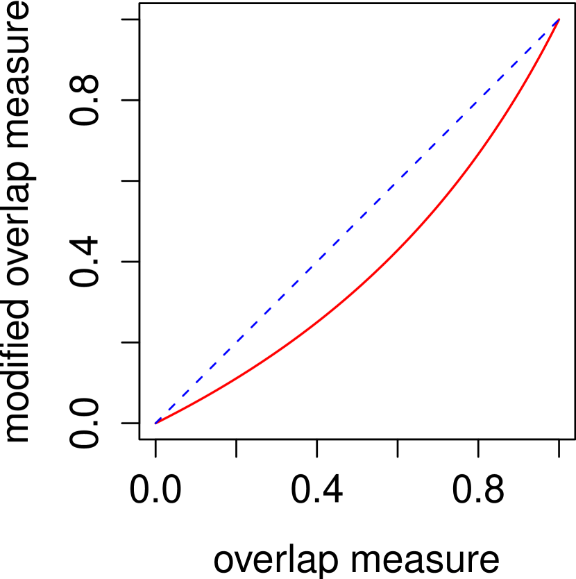
Figure 1: Plot of the modified percent overlap measure of activation (Jaccard similarity coefficient) ${}_{m}\omega$ (solid red line) against the percent overlap measure of activation (Dice coefficient) $\omega$. The half-broken blue line is the straight line passing through the origin and (1, 1).

Both $\omega_{j,l}$ and ${}_{m}\omega_{j,l}$ apply to single-subject test-retest studies as well as to cases where registered fMRI data are acquired on multiple subjects under the same experimental paradigm. Further $0\leq\omega_{j,l},{}_{m}\omega_{j,l}\leq 1$ with $\omega_{j,l}={}_{m}\omega_{j,l}=0$ when $V_{j,l}=0$ (i.e., no voxels activated in both replications) and $\omega_{j,l}={}_{m}\omega_{j,l}=1$ when $V_{j,l}=V_{j}=V_{l}$ (i.e., the same voxels are identified as activated in the $j$th and $l$th replications). However, $\omega_{j,l}$ and ${}_{m}\omega_{j,l}$ share a non-linear relationship between 0 and 1. To see this, note that dividing both the numerator and denominator in (1) by $2V_{j,l}$ for $V_{j,l}\neq 0$ yields

$${}_{m}\omega_{j,l}=\frac{\omega_{j,l}}{2-\omega_{j,l}}.$$

Since ${}_{m}\omega_{j,l}=\omega_{j,l}=0$ when $V_{j,l}=0$, this relationship holds always. Also, $\omega_{j,l}\leq 1$, so that $0\leq{}_{m}\omega_{j,l}\leq\omega_{j,l}\leq 1$, with equality only when both are zero or unity. Figure 1 shows the relationship between ${}_{m}\omega_{j,l}$ and $\omega_{j,l}$. Both ${}_{m}\omega_{j,l}$ and $\omega_{j,l}$ climb from a minimum value of zero to a maximum value of unity, but they do so at different rates. I next contend through two illustrative example scenarios that ${}_{m}\omega_{j,l}$ provides a more natural quantification of overlap. All my examples are on putative registered activation maps of dimensions $128\times 128\times 22$ voxels: thus they contain 360,448 voxels. Further, my examples are chosen to have between only 1–3.7% of active voxels in any replication, to mimic the often low rate of active voxels in an imaging study.

Illustrative Example 1

Replication A has 3,604 (1%) activated voxels while Replication B has 10,813 (3%) activated voxels, with 1,081 (0.3%) voxels commonly identified as activated in both replications, so there are $3,604+10,813-1,081=13,336$ (3.7%) voxels activated in at least one of the two replications. If our basis were these 13,336 voxels, a natural measure of coincidence is the proportion of these voxels in the overlapping area i.e., the 1,081 voxels. Now $1,081/13,336=0.081$ which is exactly ${}_{m}\omega$. This measure is therefore more intuitive than $\omega=0.150$.

Illustrative Example 2

This example has the same number of activated voxels for both replications as before, but there are 3,243 (0.9%) voxels commonly identified as activated in both replications. Here ${}_{m}\omega=0.29$ while $\omega=0.45$. The value of $\omega$ is three times that of the previous example which may, at first glance, seem appropriate – after all, there are three times more common activated voxels – but the number of commonly active voxels, is over a basis of far fewer voxels (11,174) than previously (13,336). Thus, there is far more reliability in activation than three times the previous value, as suggested by $\omega$: ${}_{m}\omega$ which at 0.29 is 3.625 times the corresponding value in the previous example, provides a better quantification of the relative sense of this reliability.

In this section, I have introduced the Jaccard similarity coefficient as a modified measure of the percent overlap of activation. I now introduce a generalized measure to summarize several percent-overlap- of-activation measures.

II-B Summarizing Several Pairwise Overlap Measures

Suppose we have $M$ activation maps, each obtained from a fMRI study under the same experimental paradigm. Define ${}_{m}\omega_{j,j}=\omega_{j,j}=1$ for $j=1,2,\ldots,M$. For each pair $(j,l);1\leq j,l\leq M$ of studies, let $\omega_{j,l}$ be the percent overlap of activation and ${}_{m}\omega_{j,l}$ be its corresponding modified version. Further, let $\Omega=\left(\left(\omega_{j,l}\right)\right)_{j=1,2,\ldots,M;l=1,2,\ldots M}$ and ${}_{m}\Omega=\left(\left({}_{m}\omega_{j,l}\right)\right)_{j=1,2,\ldots,M;l=1,2,\ldots M}$ be the matrices of the corresponding $\omega_{j,l}$s and ${}_{m}\omega_{j,l}$s. These ${}_{m}\omega_{j,l}$s and $\omega_{j,l}$s are all pairwise overlap measures which need to be summarized. Before proceeding further, I note that a generalized overlap measure between all studies could be defined in terms of the proportion of the voxels identified as activated in all replications out of those identified as activated in at least one replication; but, given the low rate of active voxels and high variability in activation in many fMRI studies, this measure would in many cases be too small to be of much practical value.  [37, page 122] have passed on a suggestion made by E. C. Pielou (in personal communication to them) in deriving a multiple Jaccard index from the pairwise indices: for large $M$, this suggestion takes a maximum value of $MS_{M}/4$, where $S_{M}$ (in our case) is the total number of voxels activated in at least one study. This generalization does not provide us with a proper sense for what constitutes a high or a low value even when $M$ is large, since the upper value depends on $S_{M}$ which can change from one set of studies to the next. For more modest-sized $M$, the maximum possible attained value is not known so that quantification is an even bigger issue. I therefore propose to derive a measure summarizing the matrix of pairwise overlaps. To fix ideas, I develop methodology here using ${}_{m}\Omega$ but emphasize that derivations are analogous for $\Omega$.

Before deriving a summarized measure over all $M$ studies, I note that there is highest reliability between them when ${}_{m}\omega_{j,l}=1$ for all $j,l\in\{1,2,\ldots,M\}$, the $M\times M$-matrix of ones. On the other hand, the worst case is when there is zero pairwise overlap between any two fMRI maps, then ${}_{m}\Omega=I_{M}$, the $M\times M$ identity matrix. Any summarized measure should assess these best- and worst-case scenarios at the two ends of the scale. I now proceed with my derivations.

Let ${}_{m}\lambda_{(1)}\geq{}_{m}\lambda_{(2)}\geq\ldots\geq{}_{m}\lambda_{(M)}$ be the eigenvalues of ${}_{m}\Omega$; these values are all real since ${}_{m}\Omega$ is a symmetric matrix. Further, the trace of ${}_{m}\Omega$ is $M$, hence ${}_{m}\lambda_{(1)}>0$. I define the summarized measure of the modified percent overlap of activation, i.e., the summarized multiple Jaccard similarity coefficient as

$${}_{m}^{s}\omega=\frac{1}{M-1}\left(M\frac{{}_{m}\lambda_{(1)}}{\sum_{i=1}^{M}{}_{m}\lambda_{(i)}}-1\right)\equiv\frac{{}_{m}\lambda_{(1)}-1}{M-1},$$ (2)

where the last equality follows from the fact that the trace of ${}_{m}\Omega$ is also equal to $\sum_{i=1}^{M}{}_{m}\lambda_{(i)}$. The motivation for this derivation comes from principal components analysis (PCA) in statistics. In PCA, the ratio of the largest eigenvalue to that of the sum of all the eigenvalues measures the proportion of variation explained by the first principal component (PC). The first PC is that projection of the data which captures the maximum amount of variability in the $M$ coordinates. PCA can be performed by obtaining a spectral decomposition of either the correlation or the covariance matrix, with differing results: since ${}_{m}\Omega$ has the flavor of a correlation matrix with unity on the diagonals and off-diagonal (nonnegative) elements of less than unity, I motivate ${}_{m}^{s}\omega$ using the analogue to the correlation matrix. When the correlation matrix is identity, the coordinates are all independent and the first PC captures only $1/M$ fraction of variability in the data. On the other hand, when the correlation matrix is equal to $J_{M}$, then all the information is carried in one coordinate: thus the first PC explains 100% of the variation in the data. When ${}_{m}\Omega=I_{M}$, all eigenvalues are the same so that the ratio of the largest eigenvalue ${}_{m}\lambda_{(1)}$ to the sum of the eigenvalues is equal to $1/M$. This is the worst-case scenario, so we shift and scale the value such that the summarized measure is zero. Alternatively, when ${}_{m}\Omega=J_{M}$, ${}_{m}\lambda_{(1)}=M$ and all other eigenvalues are zero. This is the best-case scenario, with perfect overlap between all replications, so the summary should take its highest possible value of 1: ${{}_{m}\lambda_{(1)}}/{\sum_{i=1}^{M}{}_{m}\lambda_{(i)}}$ is shifted and scaled to equal 1. Solving the two simultaneous equations for the best and worst cases yields the proposed summarized measure ${}_{m}^{s}\omega$ in (2).

Note that ${}_{m}\Omega$ is a nonnegative symmetric matrix, i.e. all entries are nonnegative. By the Perron-Frobenius theorem for nonnegative matrices (see Theorems 1.4.4 and 1.7.3 in [38]), ${}_{m}\lambda_{(1)}$ (which is also the spectral radius of ${}_{m}\Omega$) is bounded above and below by the minimum and the maximum of the row sums, respectively. All row sums of ${}_{m}\Omega$ are not less than 1 (since the diagonal elements are 1) and not greater than $M$ (since each of the $M$ elements in a row is between 0 and 1). Thus, $0\leq{}^{s}_{m}\omega\leq 1$. Further, when there are only two replications (i.e. $M=2$), ${}_{m}\Omega$ is a $2\times 2$-matrix with diagonal elements given by unity and off-diagonal elements given by ${}_{m}\omega_{1,2}\equiv{}_{m}\omega$. Trivial algebra shows that ${}_{m}\lambda_{(1)}=1+{}_{m}\omega$, so ${}_{m}^{s}\omega$ in (2) reduces to ${}_{m}\omega$ for $M=2$. Thus, the proposed ${}_{m}^{s}\omega$ is consistent with the pairwise overlap measure for $M=2$.

II-C Identifying Outlying and Anomalous Activation Maps

This section develops a testing tool using ${}_{m}^{s}\omega$ in order to identify studies that are anomalous or outliers. As before, ${}^{s}_{m}\omega$ is calculated from the $M$ studies. Further, for each $j=1,2,\ldots,M$, let ${}^{s}_{m}\omega_{-j}$ be the summarized overlap measure obtained from the $M-1$ studies with the $j$th study deleted. If the $j$th study is not very similar to the other studies, i.e. ${}_{m}\omega_{j,l}$ is low for $l\neq j$, then including it should result in a much lower ${}^{s}_{m}\omega$ than ${}^{s}_{m}\omega_{-j}$. I propose a testing scheme to flag such studies.

To do so, I advocate using as my measure

$$\zeta_{-j}=\frac{2}{\pi}\arcsin\sqrt{{}_{m}^{s}\omega_{-j}}-\frac{2}{\pi}\arcsin\sqrt{{}_{m}^{s}\omega}.$$

My motivation for applying the arcsine transformation on the ${}_{m}^{s}\omega_{-j}$ arises from the variance-stabilizing transformation $\psi(p)=\frac{2}{\pi}\arcsin\sqrt{p}$ often used to approximate the distribution of the proportion of success in binomial trials using a constant-variance normal distribution. Because $0\leq^{s}_{m}\!\!\omega\leq 1$, we have a similar framework as a proportion. However, the distributional assumption governing the form of $\zeta_{-j}$ is not known. In any case, the normal approximation (to the binomial distribution) is asymptotic and not very accurate for small $M$: therefore I propose using a jackknife test [39, 40]. I obtain a jackknifed variance estimate of $\zeta_{-j}$ for each $j=1,2,\ldots,M$. Specifically, I calculate $\zeta_{-(j,k)}=\frac{2}{\pi}\arcsin\sqrt{{}_{m}^{s}\omega_{-(j,k)}}-\frac{2}{\pi}\arcsin\sqrt{{}_{m}^{s}\omega_{-k}}$, where ${}_{m}^{s}\omega_{-(j,k)}$ is the summarized overlap measure obtained using all but the $j$th and the $k$th studies. The jackknifed variance estimator for $\zeta_{-j}$ is then given by

$${s}^{2}_{\zeta_{-j}}=\frac{1}{(M-1)(M-2)}\sum_{\begin{subarray}{c}k=1\\ k\neq j\end{subarray}}^{M}\left[\zeta_{-(j,k)}-\bar{\zeta}_{-j}\right]^{2},$$ (3)

where $\bar{\zeta}_{-j}$ is the jackknifed mean given by

$$\bar{\zeta}_{-j}=\frac{1}{M-1}\sum_{\begin{subarray}{c}k=1\\ k\neq j\end{subarray}}^{M}\zeta_{-(j,k)}.$$

The test statistic for detecting significant reduction in the summarized overlap measure upon including the $j$th study (and hence detecting if it is anomalous) is given by

$$\tau_{-j}=\frac{\zeta_{-j}}{s_{\zeta_{-j}}},$$

with $p$-value computed from the area under the $t_{M-2}$ density to the right of $\tau_{-j}$. False Discovery Rate (FDR)-controlling techniques, such as in [41] may be used to control for the proportions of expected false discoveries in detecting significant outliers.

Several comments are in order. First, I note that the multiple Jaccard index proposed in [37] is unusable in our testing strategy because its range of values changes from one set of studies to the next. My summarized multiple Jaccard similarity coefficient however takes values between zero and unity and is comparable from one set of studies to the other: thus, it can be compared across different jackknifed samples, which under the null hypothesis would have similar distributional properties. Further, the outlier detection method proposed in this section contrasts with that in [36] in that the latter draws inferences on the original post-processed time series data at each voxel.  [35] use maps of $t$-statistics or $p$-values of activation to identify outliers. My proposed approach uses downstream statistics in a similar manner as the latter, but only requires activation maps which can be acquired by any method, even methods that differ from one study to the next. In this regard, it may be considered to be a generalization of [35]’s methodology.

A reviewer has pointed out that the pairwise Jaccard similarity coefficient ${}_{m}\omega_{jl}$, while a proportion, is still a ratio of the number of voxels activated in both the $j$th and the $l$th replications to the number of voxels activated in at least one of them. This is also true of the pairwise percent overlap measure of activation proposed by [1] and [2]. The distribution of the ratios of random variables is quite complicated and can bring with it a host of issues (see, for instance, [42]). The use of the jackknife, however means that no assumptions are made on the distribution of either the numerator or the denominator in any of the pairwise measures involved in the construction of the (jackknifed) variance estimator in (3). This allays potential concerns on distributional assumptions as a consequence of using ratios of random variables.

III Illustration and Application to Motor-task Experiments

III-A Experimental and Imaging Setup

The methodology was applied to two replicated sets of experiments, with each set corresponding to right- and left-hand finger-thumb opposition tasks, performed by the same normal right-hand dominant male volunteer, after obtaining his informed consent. Each set of experiments consisted of twelve sessions conducted over a two-month period. The experimental paradigm in a session consisted of eight cycles of a simple finger-thumb opposition motor task, with the experiment performed by the right or left hand depending on whether the session was for the right- or left-hand experiment. During each cycle, the subject conducted finger-thumb opposition of the hand for 32 seconds, followed by an equal period of rest. MR images for both experiments were acquired on a GE 1.5 Tesla Signa system equipped with echo-planar gradients, with inter-session differences minimized using [15]’s recommendations on slice-positioning. For each fMRI session, a single-shot spiral sequence (TE/TR = 35/4000 ms) was used to acquire twenty-four 6 mm-thick slices parallel to the AC-PC line and with no inter-slice gap. Thus, data were collected at 128 time points. Structural $\mbox{T}_{1}$-weighted images were also acquired using a standard spin-echo sequence (TE/TR = 10/500 ms). The data were transferred from the scanner on to an SGI Origin 200 workstation where image reconstructions were performed. Motion-related artifacts in each replication were reduced via the Automated Image Registration (AIR) software using the default first image as target, and then the time series at each voxel [13] was normalized to remove linear drift. Further residual misregistration between the twelve sessions was minimized by application of inter-session registration algorithms in AFNI  [43]. Functional maps were created for each session after computing voxel-wise $t$-statistics (and corresponding $p$-values) using a general linear model, discarding the first three image volumes (to account for $\mbox{T}_{1}$ saturation effects) and assuming first-order autoregressive errors, using sinusoidal waveforms with lags of 8 seconds. The choice of waveform represented the BOLD response with the lag duration corresponding to when the response was seen after the theoretical start of the stimulus. Activation maps were drawn using the R package AnalyzeFMRI and Random Field theory and the expected Euler characteristic derivations of [44] and [45] at a significance level of 5%. The methodologies developed in this paper were applied to these maps. All computations were written using the open-source statistical software R [46].

III-B Results

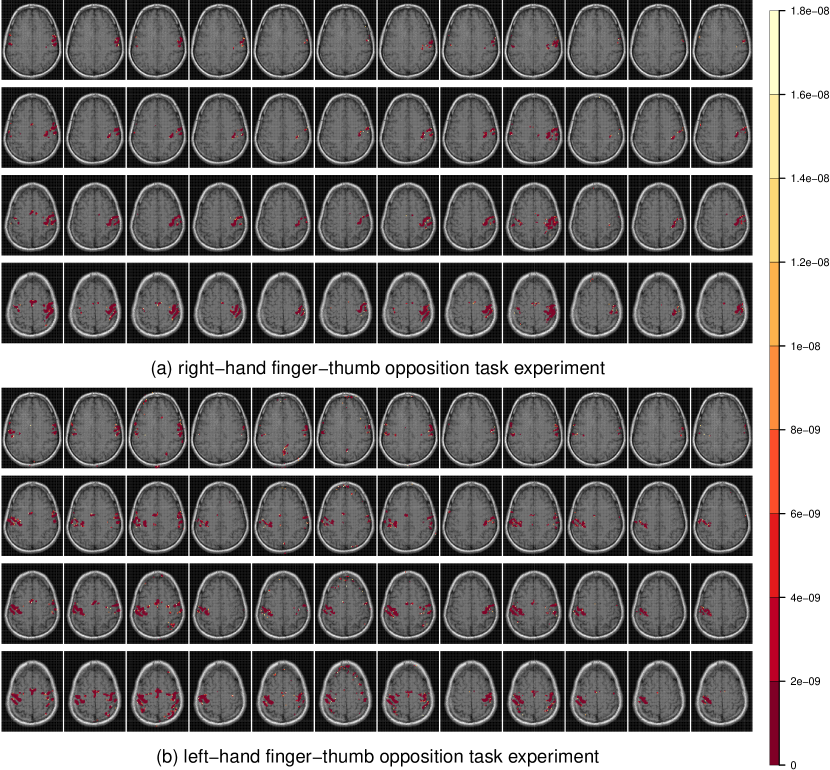
Figure 2: Radiologic view maps of observed $p$-values of activation of the $t$-test of motor function for (a) the right-hand and (b) left-hand finger-thumb opposition task experiments. For each set of experiments, we display radiologic view maps for the 18th, 19th, 20th and 21st slices (row-wise). The twelve replications are represented column-wise from 1 through 12. For each slice, we display the $p$-values of activation for the thresholded voxels using a $t$-test of the motor function for the twelve replications of the finger-thumb opposition experiment performed by (a) the right hand and (b) the left hand of the same right-hand dominant male volunteer. Note the differences in location and extent of activation over the twelve replications. Note, also the substantial more variability in the experiments performed by the subject’s left hand than on the right.

Figure 2 represents the observed $p$-values of activation for slices 18, 19, 20 and 21 (row-wise) over the twelve replications for both the (a) right-hand and (b) left-hand finger-thumb opposition tasks. (All displayed maps in this paper are in radiologic views and overlaid on top of the corresponding $\mbox{T}_{1}$-weighted anatomical images.) The specific slices were chosen for display because they encompass the ipsi- and contra-lateral pre-motor cortices (pre-M1), the primary motor cortex (M1), the pre-supplementary motor cortex (pre-SMA), and the supplementary motor cortex (SMA). Clearly, there is some variability in the results for the right-hand task. In Figure 2a for instance, all experiments identify activation in the left M1 and in the ipsi-lateral pre-M1 areas, but there is some modest variability in the identified activation in the contra-lateral pre-M1, pre-SMA and SMA voxels, with some experiments reporting very localized or no activation and others having these regions as activated and somewhat diffused in extent. Slices for the left-hand finger-thumb opposition task experiments in Figure 2b, on the other hand, show far more variability, both in location and extent. It is interesting to note that while most experiments identify activation in the right M1, the ipsi-lateral, contra-lateral pre-M1, pre-SMA and SMA areas, they also often show activation in the corresponding left regions. The case of the eighth replication is extremely peculiar. Most of the activity in the four slices are in the left areas and the right areas have little to no activation. This makes one wonder if the naturally right-hand dominant male volunteer had, perhaps unintentionally and out of habit, used his right hand instead of his left in performing some part of the experimental paradigm. In summary, there is clearly far more variability in the left hand set of experiments than in the right hand set. We now assess the reliability in each set separately.

III-B1 Reliability of right-hand finger-thumb opposition task experiments

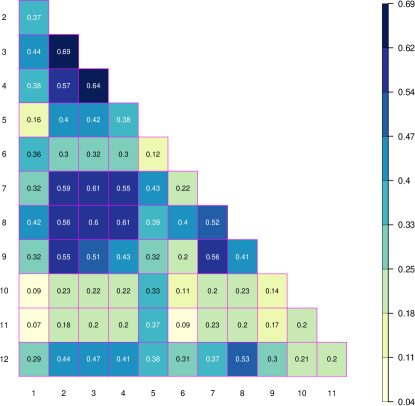
(a) $\Omega$

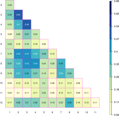
(b) ${}_{m}\Omega$

Figure 3: Display of overlap measures on the right-hand finger-thumb-opposition task experiment, obtained using (a) [1] and [2]’s $\Omega$ and its (b) modified Jaccard similarity coefficient version ${}_{m}\Omega$ as proposed in this paper.

Figure III-B1 displays the lower triangle of the matrix pairwise per cent overlap measures of activation calculated as per (a) [1] and [2] and (b) the Jaccard similarity coefficient modification suggested in this paper. As proved in Section II-A, ${}_{m}\Omega\leq\Omega$, entry-wise. The (3,2) pair of experiments has the highest percent overlap of activation, with ${}_{m}\omega_{3,2}=0.524$ while $\omega_{3,2}=0.688$. Compared to other values of $j$, the low ${}_{m}\omega_{j,l}$ values for $j=10$ or 11 are striking! While $\omega_{j,l}$s are lower for $j=10,11$ than for other $j$, they are not as pronounced as ${}_{m}\omega_{j,l}$. This points to the possibility that activation maps obtained using these replications may be somewhat different from the others. Using the methodology of Section II-B provides us with the summarized measures ${}_{m}^{s}\omega=0.244$ and ${}^{s}\omega=0.372$. We now investigate performance of the methodology of Section II-C in flagging potential outliers or anomalous studies.

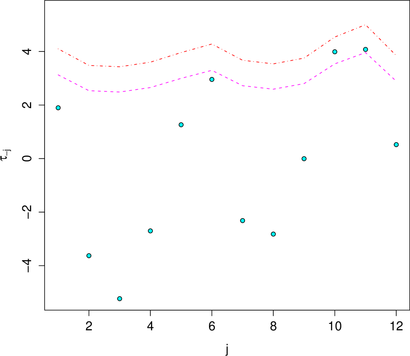
Figure 4: Plot of $\tau_{-j}$ against $j$ for the right-hand finger-thumb opposition task experiment. The half-broken and semi-solid lines displays thresholds obtained when controlling eFDR at $q=0.05$ and $q=0.01$, respectively.

The coefficient of variation in the jackknife-estimated standard deviations of $\hat{\zeta}_{-j}$s was around 0.0501: this indicates that the arc-sine transformation was able to stabilize the variance substantially. Figure 4 plots the computed $\tau_{-j}$ against $j$ for each $j=1,2,\ldots,12$. Note that the values of $\tau_{-10}$ and $\tau_{-11}$ are fairly high: indeed, the corresponding fMRI maps would be identified as significant outliers if we used an expected FDR (eFDR) of $q=0.05$, but not so using an eFDR of $q=0.01$. Thus they may be considered to be moderate outliers: this finding is in keeping with the general impression we obtained from Figure 2a. Eliminating the moderate outliers increases the summarized overlap measure: ${}^{s}_{m}\omega_{-(10,11)}=0.287$ (${}^{s}\omega_{-(10,11)}=0.432$). Figure 5a and b displays the composite activation map obtained upon combining all the replications and all but the tenth and eleventh replications, respectively. Each composite map was obtained by averaging the $t$-statistics for each study [47] and determining activation as before using the Random Field theory of [45] at 5% significance. The activated regions in Figure 5b are slightly more defined than in Figure 5a. This makes sense because the effects of the less reliable studies have been removed in constructing the composite activation map of Figure 5b.

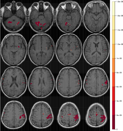
Figure 5: Composite activation map for slices 7 through 22, of the right-hand finger-thumb opposition task experiment obtained using (a) all twelve fMRI studies and (b) all but the tenth and eleventh studies. Displays are as in Figure 2.

III-B2 Reliability of left-hand finger-thumb opposition task experiments

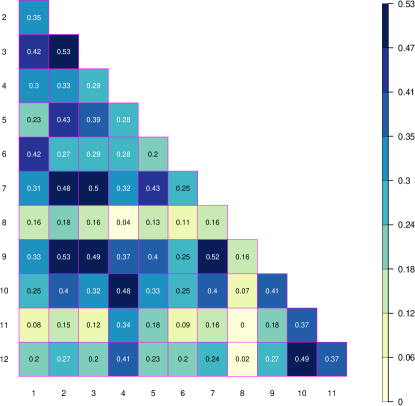
(a) $\Omega$

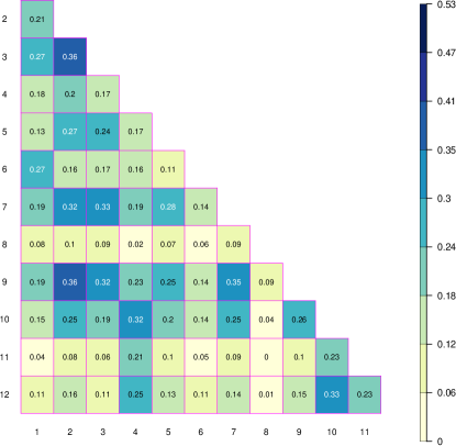
(b) ${}_{m}\Omega$

Figure 6: Display of overlap measures on the left-hand finger-thumb-opposition task experiment, obtained using (a) [1] and [2]’s percent overlap measures of activated and their (b) modified (Jaccard similarity coefficient) versions as proposed in this paper. Displays are analogous to Figure III-B1.

Figure III-B2 displays the lower triangle of $\Omega$ and ${}_{m}\Omega$ for this set of experiments. Once again, ${}_{m}\Omega\leq\Omega$ element-wise. The second and the ninth replications have the highest percent overlap of activation (${}_{m}\omega_{9,2}=0.361$ and $\omega_{9,2}=0.531$) while there is hardly any overlap between the eighth and the eleventh replications (${}_{m}\omega_{11,8}=0.002$, $\omega_{11,8}=0.004$). In general, the values of ${}_{m}\omega_{8,j}$ (and $\omega_{8,j}$) are very low for all $j\neq 8$ and in line with our suspicions from studying Figure 2b. The graphical representation of $\omega_{8,2}$ and ${}_{m}\omega_{8,2}$ in Figure III-B2 presents the case for using ${}_{m}\omega$ over $\omega$ very well. In Figure III-B2a, the value of $\omega_{8,2}$ is in the middle third of the scale for $\Omega$: thus, the graphical display would cause us to hesitate before declaring that the activation identified in the eighth and second replications are very different from each other. However, Figure 2b does not provide much justification for such second thoughts, corroborating the value of ${}_{m}\omega{8,2}$ (which is in the lower third of the values graphically displayed in Figure III-B2b). Values of ${}_{m}\omega_{11,j}$ (and $\omega_{11,j}$) are also low for all $j\neq 11$ even though they are a bit higher than for ${}_{m}\omega_{8,j}$ and $\omega_{8,j}$. The summarized measure over all twelve replications was ${}^{s}_{m}\omega=0.187$ and ${}^{s}\omega=0.303$. Thus, there is far less reliability in identified activation in this set of experiments relative to the right-hand set. We now identify potentially anomalous fMRI studies in the left-hand set.

Once again, the coefficient of variation in the jackknife-estimated standard deviations of $\zeta_{-j}$ is small, around 0.093 so that the variance stabilizing transformation is seen to do a good job in terms of homogenizing variances in both sets of our experiments. Figure 7 plots $\tau_{-j}$ against $j$. Note that $\tau_{-8}$ is significant even when controlling eFDR at $q=0.01$. The eighth study is thus an extreme outlier. The eleventh replication is, however, a moderate outlier. Deleting the eighth replication yields ${}^{s}_{m}\omega_{-8}=0.204$ (${}^{s}\omega_{-8}=0.329$) while deleting the moderate and extremely anomalous studies results in ${}^{s}_{m}\omega_{-(8,11)}=0.219$ (${}^{s}\omega_{-(8,11)}=0.351$).

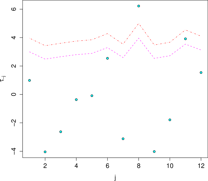
Figure 7: Plot of $\tau_{-j}$ against $j$ for the left-hand finger-thumb opposition task experiment, with displays as in Figure 4.

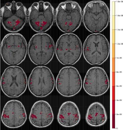
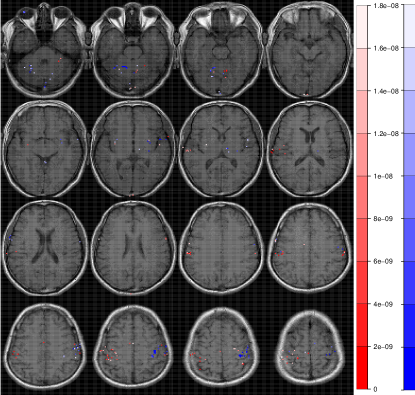
Figure 8: Composite activation maps obtained using (a) all studies and (b) all but the eighth fMRI study for the left-hand finger-thumb opposition task experiment. Displays are as in Figure 2. (c) Difference in the composite activation maps of (a) and (b). Blue-hued voxels are those that were identified as activated in (a) but not in (b) while red-hued voxels are those identified as activated in (b) but not in (a). In both cases, hue is proportional to the $p$-value of the test statistic when it was identified as significant.

Figures 8a and b display the composite activation maps for the left-hand set by combining all studies and all but the eighth studies, respectively. Figure 8c shows voxels that were differentially activated in the two composite maps. Slices 18 through 21 have more significant voxels in the left areas of (a) than in (b) and fewer significant voxels in the right areas of (a) than in (b). There is therefore increased localization in the identified activation when the eighth study is excluded.

III-B3 Sensitivity to thresholding values

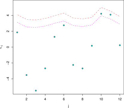
(a) right-hand experiments, $\alpha=0.01$

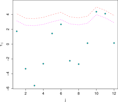
(b) right-hand experiments, $\alpha=0.001$

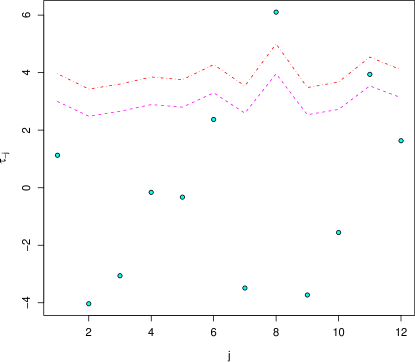
(c) left-hand experiments, $\alpha=0.01$

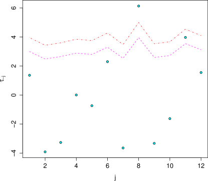
(d) left-hand experiments, $\alpha=0.001$

Figure 9: Plot of $\tau_{-j}$ against $j$ at thresholding values of (a, c) $\alpha=0.01$ and (b, d) $\alpha=0.001$ for (a, b) the right- and (c, d) left-hand finger-thumb opposition task experiments. Displays are as in Figure 4.

A reviewer has very kindly pointed out that the outliers identified in Sections III-B1 and III-B2 are from fMRI activation maps drawn using Random Field theory and at a significance threshold of $\alpha=0.05$. The methodology was therefore applied to activation maps drawn using the same approach but with more conservative significance thresholding ($\alpha=0.01$ and $\alpha=0.001$). Figure 9 displays the $\tau_{-j}$’s obtained from activation maps at the two significance thresholds for the right- and the left-hand experiments. The tenth and eleventh fMRI studies are again the only ones identified as moderately anomalous for the right-hand experiments at both $\alpha=0.01$ and $\alpha=0.001$. As before, the eighth fMRI study is also the only extreme outlier in the left-hand set while the eleventh study is the only moderate outlier. The outlier-detection strategy thus appears to be remarkably robust to the exact significance thresholding selected in creating our fMRI maps.

In this section, I have demonstrated use of the Jaccard similarity coefficient as a modified measure for the pairwise percent overlap of activation and shown that it can provide a better sense of reliability. I have also illustrated the use of my summary measure for quantifying the overall percent overlap of activation from multiple fMRI studies. Finally, I have illustrated the utility of the developed testing tool to identify potentially anomalous fMRI maps and have also shown that it is fairly robust to different choices of thresholding used in the preparation of fMRI activation maps.

IV Discussion

[1] and [2] have proposed a measure of the percent overlap in voxels that are identified as activated in any pair of replications. Although novel in the context of studying fMRI reproducibility, this measure is the same as the Dice coefficient [27, 28] which is known to have several drawbacks. This paper has investigated use of the Jaccard similarity coefficient by slightly modifying the  [1] and [2] measure. The modified measure is seen to incorporate a more intuitive set theoretic interpretation, which is demonstrated through some illustrative examples as well as through application to two replicated fMRI datasets. A summarized percent overlap measure of activation (the summarized multiple Jaccard similarity coefficient) for quantifying reliability of activation over multiple fMRI studies has also been proposed. A testing strategy has also been developed that uses improvements in the summarized multiple Jaccard similarity coefficient upon excluding studies to evaluate whether a particular study is an outlier or an anomaly and should be discarded from the analysis. Although developed and demonstrated on test-retest studies with replicated activation maps on a single subject, the methodology is general enough to apply to multi-subject fMRI data.

We have applied our developed methodologies to two sets of replicated experiments performed by the same right-hand-dominant normal male volunteer. The two sets of experiments pertained to finger-thumb opposition tasks performed by the subject using his right and his left hand respectively. Our summarized measures of percent overlap of activation are substantially higher for the right-hand task than for the left-hand task. This agrees with the visual cues provided in Figure 2 where we noticed substantially more variability in the activation maps for the left-hand task experiments than for the right-hand ones. We have further used our testing strategy to flag down potentially anomalous replications: for the right-hand task experiment, there were two moderately anomalous studies. For the set of experiments on the left-hand tasks, the eighth replication was an extreme anomaly while the eleventh study was moderately anomalous. Deleting these studies resulted in both increased localization and spatial extent of the composite fMRI maps. Finally, the outlier detection was seen to be remarkably insensitive to the choice of thresholding used in the creation of the original activation maps.

There are a number of benefits that our suggested testing mechanism for flagging anomalous studies provides. A study identified as a potential outlier may trigger further investigation since there are several reasons why a study may be flagged as anomalous. For one, it may point to physical issues with regard to the scanner. Alternatively, and in the context of multi-subject studies, this may be useful for clinical diagnosis: for example, it may be worth investigating why a particular subject had a very different activation map. In other words, this can point the researcher and the neurologist to the need for further clinical investigation and diagnosis. In the testing scheme developed in Section II-C, we only evaluated the effect of removing one observation at a time. It would be interesting to investigate the effect of removing multiple observations. Another avenue worth pursuing is the development of similar measures for grouped fMRI studies. Thus, while this paper has made a promising contribution, several issues meriting further attention remain.

V Acknowledgments

I am very grateful to the Section Editor, the Handling Editor and three reviewers whose very detailed and insightful comments on an earlier version of this manuscript greatly improved its quality. I thank Rao P. Gullapalli of the University of Maryland School of Medicine for providing me with the data used in this study. This material is based, in part, upon work supported by the National Science Foundation (NSF) under its CAREER Grant No. DMS-0437555 and by the National Institutes of Health (NIH) under its Grant No. DC-0006740.

References

- [1] S. A. Rombouts, F. Barkhof, F. G. Hoogenraad, M. Sprenger, and P. Scheltens, “Within-subject reproducibility of visual activation patterns with functional magnetic resonance imaging using multislice echo planar imaging,” Magnetic Resonance Imaging, vol. 16, pp. 105–113, 1998.
- [2] W. C. Machielsen, S. A. Rombouts, F. Barkhof, P. Scheltens, and M. P. Witter, “fMRI of visual encoding: reproducibility of activation,” Human Brain Mapping, vol. 9, pp. 156–64, 2000.
- [3] P. Jaccard, “Ètude comparative de la distribution florale dans une portion des alpes et des jura,” Bulletin del la Sociètè Vaudoise des Sciences Naturelles, vol. 37, p. 547–579, 1901.
- [4] B. Biswal, A. E. DeYoe, and J. S. Hyde, “Reduction of physiological fluctuations in fMRI using digital filters.” Magn Reson Med, vol. 35, no. 1, pp. 107–113, January 1996. [Online]. Available: http://view.ncbi.nlm.nih.gov/pubmed/8771028
- [5] C. R. Genovese, D. C. Noll, and W. F. Eddy, “Estimating test-retest reliability in functional MR imaging: I. Statistical methodology,” Magnetic Resonance in Medicine, vol. 38, pp. 497–507, 1997.
- [6] J. V. Hajnal, R. Myers, A. Oatridge, J. E. Schweiso, J. R. Young, and G. M. Bydder, “Artifacts due to stimulus-correlated motion in functional imaging of the brain,” Magnetic Resonance in Medicine, vol. 31, pp. 283–291, 1994.
- [7] R. Maitra, S. R. Roys, and R. P. Gullapalli, “Test-retest reliability estimation of functional mri data,” Magnetic Resonance in Medicine, vol. 48, pp. 62–70, 2002.
- [8] E. E. Chen and S. L. Small, “Test-retest reliability in fMRI of language: Group and task effects,” Brain and Language, vol. 102, no. 2, pp. 176–85, 2007. [Online]. Available: http://dx.doi.org/10.1016/j.bandl.2006.04.015
- [9] B. R. Buchsbaum, S. Greer, W. L. Chang, and K. F. Berman, “Meta-analysis of neuroimaging studies of the wisconsin card-sorting task and component processes,” Human Brain Mapping, vol. 25, pp. 35–45, 2005.
- [10] J. Derrfuss, M. Brass, J. Neumann, and D. Y. von Cramon, “Involvement of inferior frontal junction in cognitive control: meta-analyses of switching and stroop studies,” Human Brain Mapping, vol. 25, pp. 22–34, 2005.
- [11] K. R. Ridderinkhof, M. Ullsperger, E. A. Cron, and S. Nieuwenhuis, “The role of the medial frontal cortex in cognitive control,” Science, vol. 306, pp. 443–447, 2004.
- [12] W. R. Uttal, The new phrenology: the limits of localizing cognitive processes in the brain. Cambridge, MA: The MIT Press, 2001.
- [13] R. P. Wood, S. T. Grafton, J. D. G. Watson, N. L. Sicotte, and J. C. Mazziotta, “Automated image registration. ii. intersubject validation of linear and non-linear models,” Journal of Computed Assisted Tomography, vol. 22, pp. 253–265, 1998.
- [14] D. J. McGonigle, A. M. Howseman, B. S. Athwal, K. J. Friston, R. S. J. Frackowiak, and A. P. Holmes, “Variability in fMRI: an examination of intersession differences,” Neuroimage, vol. 11, pp. 708–734, 2000.
- [15] F. C. Noll, C. R. Genovese, L. E. Nystrom, A. L. Vazquez, S. D. Forman, W. F. Eddy, and J. D. Cohen, “Estimating test-retest reliability in functional MR imaging. II. Application to motor and cognitive activation studies,” Magnetic Resonance in Medicine, vol. 38, pp. 508–517, 1997.
- [16] X. Wei, S. S. Yoo, C. C. Dickey, K. H. Zou, C. R. Guttman, and L. P. Panych, “Functional MRI of auditory verbal working memory: long-term reproducibility analysis,” Neuroimage, vol. 21, pp. 1000–1008, 2004.
- [17] P. E. Shrout and J. L. Fleiss, “Intraclass correlations: Uses in assessing rater reliability,” Psychological Bulletin, vol. 86, no. 2, pp. 420–428, 1979.
- [18] G. G. Koch, “Intraclass correlation coefficient,” in Encyclopedia of Statistical Sciences, S. Kotz, , and N. L. Johnson, Eds., vol. 4. New York: John Wiley and Sons, 1982, pp. 213–217.
- [19] K. O. McGraw and S. P. Wong, “Forming inferences about some intraclass correlation coefficients,” Psychological Methods, vol. 1, no. 1, pp. 30–46, 1996.
- [20] A. R. Aron, D. Shohamy, J. Clark, C. Myers, M. A. Gluck, and R. A. Poldrack, “Human midbrain sensitivity to cognitive feedback and uncertainty during classification learning,” Journal of Neurophysiology, vol. 92, pp. 1144–1152, 2004.
- [21] G. Fernández, K. Sprecht, S. Weis, I. Tendolkar, M. Reuber, J. Fell, K. P., J. Ruhlmann, J. Reul, and C. E. Elger, “Intrasubject reproducibility of presurgical language lateralization and mapping using fMRI,” Neurology, vol. 60, pp. 969–975, 2003.
- [22] L. Friedman, H. Stern, G. G. Brown, D. H. Mathalon, J. Turner, G. H. Glover, R. L. Gollub, J. Lauriello, K. O. Lim, T. Cannon, D. N. Greve, H. J. Bockholt, A. Belger, B. Mueller, M. J. Doty, J. He, W. Wells, P. Smyth, S. Pieper, S. Kim, M. Kubicki, M. Vangel, and S. G. Potkin, “Test-retest and between-site reliability in a multicenter fMRI study,” Human Brain Mapping, vol. 29, no. 8, pp. 958–972, 2008. [Online]. Available: http://dx.doi.org/10.1002/hbm.20440
- [23] D. S. Manoach, E. F. Halpern, T. S. Kramer, Y. Chang, D. C. Goff, S. L. Rauch, D. N. Kennedy, and R. L. Gollub, “Test-retest reliability of a functional MRI working memory paradigm in normal and schizophrenic subjects,” American Journal of Psychiatry, vol. 158, pp. 955–958, 2001.
- [24] F. M. Miezin, L. Maccotta, J. M. Ollinger, S. E. Petersen, and R. L. Buckner, “Characterizing the hemodynamic response: effects of presentation rate, sampling procedure, and the possibility of ordering brain activity based on relative timing,” Neuroimage, vol. 11, pp. 735–759, 2000.
- [25] M. Raemekers, M. Vink, B. Zandbelt, R. J. A. van Wezel, R. S. Kahn, and N. F. Ramsey, “Test-retest reliability of fMRI activation during prosaccades and antisaccades,” Neuroimage, vol. 36, pp. 532–542, 2007.
- [26] K. Sprecht, K. Willmes, N. J. Shah, and L. Jäncke, “Assessment of reliability in functional imaging studies,” Journal of Magnetic Resonance Imaging, vol. 17, pp. 463–471, 2003.
- [27] L. R. Dice, “Measures of the amount of ecologic association between species,” Ecology, vol. 26, pp. 297–302, 1945.
- [28] T. Sørensen, “A method of establishing groups of equal amplitude in plant sociology based on similarity of species and its application to analyses of the vegetation on danish commons,” Biologiske Skrifter / Kongelige Danske Videnskabernes Selskab, vol. 5, no. 4, p. 1–34, 1948.
- [29] R. E. Tulloss, “Assessment of similarity indices for undesirable properties and a new tripartite similarity index based on cost functions,” in Mycology in Sustainable Development: Expanding Concepts, Vanishing Borders, M. E. Palm and I. H. Chapela, Eds. North Carolina: Parkway Publishers, 1997, pp. 122–143.
- [30] S. Ruddell, S. Twiss, and P. Pomeroy, “Measuring opportunity for sociality: quantifying social stability in a colonially breeding phocid,” Animal Behaviour, vol. 74, pp. 1357–1368, 2007.
- [31] M. Levandowsky and D. Winter, “Distance between sets,” Nature, vol. 234, pp. 34–35, 1971.
- [32] F. Kherif, J.-B. Poline, S. Meriaux, H. Benali, G. Flandin, and M. Brett, “Group analysis in functional neuroimaging: selecting subjects using similarity measures,” Neuroimage, vol. 20, no. 4, pp. 2197–2208, 2003.
- [33] W.-L. Luo and T. E. Nichols, “Diagnosis and exploration of massively univariate neuroimaging models,” Neuroimage, vol. 19, no. 3, pp. 1014–1032, 2003.
- [34] M. Seghier, K. Friston, and C. Price, “Detecting subject-specific activations using fuzzy clustering,” Neuroimage, vol. 36, pp. 594–605, 2007.
- [35] R. L. McNamee and N. A. Lazar, “Assessing the sensitivity of fMRI group maps,” Neuroimage, vol. 22, no. 2, pp. 920–931, 2004.
- [36] M. Woolrich, “Robust group analysis using outlier inference,” Neuroimage, vol. 41, pp. 286–301, 2008.
- [37] R. K. Colwell and J. A. Coddington, “Estimating terrestrial biodiversity through extrapolation,” Philosophical Transactions of the Royal Society of London, vol. 345, pp. 101–118, 1994.
- [38] R. B. Bapat and T. E. S. Raghavan, Nonnegative Matrices and Applications. Cambridge, United Kingdom: Cambridge University Press, 1997.
- [39] B. Efron, “Bootstrap methods: another look at the jackknife,” Annals of Statistics, vol. 7, pp. 1–26, 1979.
- [40] B. Efron and G. Gong, “A leisurely look at the bootstrap, the jackknife, and cross-validation,” American Statistician, vol. 37, no. 1, pp. 36–48, 1983.
- [41] Y. Benjamini and Y. Hochberg, “Controlling the false discovery rate: A practical and powerful approach to multiple testing,” Journal of the Royal Statistical Society. Series B (Methodological), vol. 57, no. 1, pp. 289–300, 1995. [Online]. Available: http://dx.doi.org/10.2307/2346101
- [42] D. B. Allison, F. Paultre, M. I. Goran, E. T. Poehlman, and S. B. Heymseld, “Statistical considerations regarding the use of ratios to adjust data,” International Journal of Obesity, vol. 19, pp. 644–652, 1995.
- [43] R. W. Cox and J. S. Hyde, “Software tools for analysis and visualization of fMRI data,” NMR in Biomedicine, vol. 10, no. 4-5, pp. 171–178, 1997.
- [44] R. Adler, The geometry of random fields. New York: Wiley, 1981.
- [45] K. J. Worsley, “Local maxima and the expected euler characteristic of excursion sets of , and fields,” Advances in Applied Probability, vol. 26, pp. 13–42, 1994.
- [46] R Development Core Team, R: A Language and Environment for Statistical Computing, R Foundation for Statistical Computing, Vienna, Austria, 2009, ISBN 3-900051-07-0. [Online]. Available: http://www.R-project.org
- [47] N. A. Lazar, B. Luna, J. A. Sweeney, and W. F. Eddy, “Combining brains: a survey of methods for statistical pooling of information,” Neuroimage, vol. 15, pp. 538–50, 2002.