Tempered, Anti-trunctated, Multiple Importance Sampling

Abstract

Importance sampling is a Monte Carlo method that introduces a proposal distribution to sample the space according to the target distribution. Yet calibration of the proposal distribution is essential to achieving efficiency, thus the resort to adaptive algorithms to tune this distribution. In the paper, we propose a new adpative importance sampling scheme, named Tempered Anti-truncated Adaptive Multiple Importance Sampling (TAMIS) algorithm. We combine a tempering scheme and a new nonlinear transformation of the weights we named anti-truncation. For efficiency, we were also concerned not to increase the number of evaluations of the target density. As a result, our proposal is an automatically tuned sequential algorithm that is robust to poor initial proposals, does not require gradient computations and scales well with the dimension.

1 Introduction

Importance sampling is a Monte Carlo method that predates Markov Chain Monte Carlo (MCMC). It was and is still used to sample distributions. importance sampling targets $\pi(x)$ with draws from the proposal distribution $q(x)$. A draw $x$ is weighted with $\pi(x)/q(x)$ to correct the discrepancy between $q$ and $\pi$. When $\pi\ll q$, these algorithms are unbiased. Moreover, when the density of the target $\pi(x)$ is known up to a constant, we normalized the weights by their sum, which introduce a small bias that has been well studied [see, e.g. 18]. Unlike MCMC, importance sampling is an embarrassingly parallel algorithm that can easily be distributed on CPU cores or clusters. Moreover, importance sampling does not require to sort the wheat from the chaff by finding the limit of the warm-up or burn-in period. And, since it is not based on local moves, it may be able to discover the different modes of the target. It has therefore received a recent interest, in particular when considering algorithms that calibrates the tuning parameters of the algorithm to the target [3].

The efficiency of importance sampling depends heavily on the choice of the proposal. Many adaptive algorithms [15, 16] have been proposed to calibrate the proposal based on past samples from the target. Thus a temporal dimension is introduced in these algorithms to adapt the tuning parameters of the proposal distribution: at time $t$, draws $x$ are sampled from a distribution $q_{t}(x)=q(x|\theta_{t})$ whose parameter $\theta_{t}$ is adapted on past results. However these algorithms suffer from numerical instability and sensibility to the first proposal used at initialization. For instance, Liu, [12, Section 2.6] claimed that such algorithms were unstable. Indeed estimating large covariance matrices from weighted samples can lead to ill-conditioned estimation problems [see, e.g., 7]. And Cornuet et al., [5] asserted that the initial distribution of their algorithm has a major impact on the accuracy of adaptive algorithms. They talked about the “what-you-get-is-what-you-see” nature of such algorithms: these methods have to guess which part of the space is charged by the target based on points of this space that have been previously visited. Several schemes have been introduced to initialise the first proposal distribution. The initialization method proposed by Cornuet et al., [5, Section 4] requires multidimensional simplex optimization, hence requires many evaluations of $\pi(\theta)$ that are then discarded. On the other hand, Beaujean and Caldwell, [1] runs a complete Metropolis-Hastings algorithm that can miss several modes of the target since it is based on local moves.

Numerical instability may come from the fact that the adaptive algorithm can be trapped around a point of the space that better fits the target than previously visited points. When such phenomenon occurs, the algorithm misses important parts of the core of the target: the learnt proposal distribution becomes concentrated around this point, and the rest of the space to sample is eliminated forever. When the space to sample is of moderate or large dimension, numerical instability becomes a major problem. Many ideas were proposed to tackle the issue including tempering and clipping [3]. Tempering [6, 11] can be implemented as replacing the target $\pi(x)$ by $\pi(x)^{\beta}$, with $\beta<1$. It eases the discovery of the core of the target since it extends the part of the space that is charged by the target. Thus, tempering can smooth the bridge from the first proposal $q_{1}(x)$ to the target $\pi(x)$. Clipping [9, 10, 19] of the importance weights is a non linear transformation of the weights that decreases the importance of points with high $w(x)=\pi(x)/q_{t}(x)$. The most common way to implement clipping as a variance reduction method (which introduce a bias) is the truncation that deals with the degeneracy as follows. If $w(x)>S$ where $S$ is a threshold that needs to be calibrated, the weights $w(x)$ are replaced by some value (e.g., by $S$). Otherwise, they are left unchanged. As noted by Koblents and Míguez, [10] and Bugallo et al., [3], this transformation of the weights flattens the target distribution. Therefore, truncation is redundant with tempering. Finally, in order to increase computational efficiency, schemes have been introduced to recycle the successive samples generated at every iterations. In this vein, Cornuet et al., [5], Marin et al., [13] considered the whole set of draws from the different proposals calibrated at each stage of the algorithm as drawn from a mixture of these distributions to significantly increase their efficiency.

In this paper, we propose an adaptive importance sampling whose sensitivity to the first proposal, and numerical instability are highly reduced. We have tried to design our algorithm to keep control on the number of evaluations of the (unnormalized) target density. In many situations where we are interested in sampling the posterior distribution, the target density is indeed a complex function of the paramaters $x$ and the data. For instance, an extreme case is a Gaussian model whose average $\mu(x)$ is a blackbox function which carries a physical model of the reality given the value of the parameters $x$. Thus, the time complexity of our algorithm should be assessed in number of evaluations of the proposal density. We relied on a simple form of tempering to adapt the proposal distribution. Nevertheless tempering was not enough to stabilize the algorithm on spaces of large dimension. In our algorithm, at each stage after initialization, we update the proposal using tempering, and an anti-truncation that replaces all weights $w(x)$ lower than a threshold $s$ by $s$. We show that this kind of clipping can be considered as a contamination of the current proposal with the previous one. As exhibited in the numerical simulations in the last Section, both tricks (tempering and contamination with previous proposal) avoid focusing too quickly on the few points with high weights. At least, our method keeps the variance of the proposal large enough to take time to explore the space to sample before exploiting the points with high importance weights.

2 Calibration of importance sampling

We propose here a new strategie to walk on the bridge from the first proposal $q_{1}(x)$ to a proposal $q_{T}(x)$ well adapted to the target $\pi(x)$ in terms of effective sample size. In order to adapt the proposal gradually, we introduce a sequence of temporary targets:

$$\widehat{\pi}_{1}(x),\ldots,\widehat{\pi}_{T}(x)$$

which are intermediaries between the first proposal $q_{1}(x)$ and the target $\pi(x)$. The precise definition of these temporary targets, given in Section 2.2, is paramount to the succes of the algorithm. They are based on a tempering $w^{\beta}$ of the importance weights $w$. As described in Section 2.1, the tempering

1. eases the discovery of the area charged by the real target $\pi(x)$,

2. temporarily removes the problems due to large queues of the target,

3. allows us to design a diagnostic based on the final of $\beta$.

To this non-linear transformation of the weights, we add an anti-truncation, defined as $\widehat{w}^{\beta}=w^{\beta}\vee s$, that pulls up all tempered weights $w^{\beta}$ less than a threshold $s$ to this single value, see Section 2.2. This anti-truncation

1. performs a contamination of the temporary target by the last proposal,

2. helps to stabilize numerically the algorithm and

3. allows us to explore new directions in large-dimension spaces.

Both $\beta$ and $s$ are automatically calibrated at the end of stage $t$ of the algorithm, as explained in Section 3.1. The new proposal $q_{t+1}(x)$ is tuned to fit the temporary $\widehat{\pi}_{t}(x)$ with the EM algorithm as given in Section 2.3. The whole algorithm is given in Figure 1.

Figure 1: The tempered, anti-truncated multiple importance sampling (TAMIS) algorithm

2.1 The tempering

Let us assume that, given all past draws, a set $x_{t,1},\ldots,x_{t,N_{t}}$ of size $N_{t}$ has been drawn independently from a distribution $q_{t}(x)=q(x|\theta_{t})$ picked among a parametric family $\mathscr{Q}$ of laws. The importance weights at this stage are

$$w_{t,i}=\frac{\pi(x_{t,i})}{q_{t}(x_{t,i})}.$$ (1)

We can replace the target $\pi(x)$ by the distribution of density

$$\pi_{\beta,t}(x)\propto\pi(x)^{\beta}q_{t}(x)^{1-\beta}$$ (2)

with inverse temperature $\beta\in(0,1)$ as proposed by Neal, [14] in his Annealed importance sampling. When $\beta=0$, (2) is the proposal distribution that served to draw the $x_{t,i}$’s: $\pi_{\beta=0,t}(x)=q_{t}(x)$. When $\beta=1$, (2) is the target distribution: $\pi_{\beta=1,t}(x)=\pi(x)$. Moreover, $\beta\mapsto\operatorname{KL}(\pi\|\pi_{\beta,t})$ decreases from $\operatorname{KL}(\pi|q_{t})$ to $0$, see Proposition 3 in A. If we use the $x_{t,i}$’s to target $\pi_{\beta,t}(x)$, the unnormalized importance weights become

$$\frac{\pi_{\beta,t}(x_{t,i})}{q_{t}(x_{t,i})}\propto\frac{\pi(x)^{\beta}q_{t}(x)^{1-\beta}}{q_{t}(x_{t,i})}=\left(\frac{\pi(x)}{q_{t}(x_{t,i})}\right)^{\beta}=w_{t,i}^{\beta}.$$ (3)

Such weights have been use in the past, for instance by Koblents and Míguez, [10] who relied on the $x_{t,i}$’s weighted with the $w_{t,i}^{\beta}$’s to get a sample from $\pi_{\beta,t}(x)$ and to tune a $q_{t+1}(x)=q(x|\theta_{t+1})$ that approximates $\pi_{\beta,t}(x)$. It is also explored by Korba and Portier, [11] as a regularization strategy.

2.2 Anti-trunctation and temporary targets

There are many ways to contaminate this weighted sample with draws from $q_{t}(x)$. The first idea is to add $N_{t}^{\prime}$ new draws $x_{t,N_{t}+1},x_{t,N_{t}+2}\ldots$ with all weights equal to $s$ to the above weighted sample. This idea may add a non negligeable amount of computational time when the dimension of $x$ is large. Another idea to contaminate this weighted sample with $q_{t}(x)$, is to change the weights. We introduce a deterministic contamination based on the value of $w_{t,i}^{\beta}$. Indeed, the $x_{t,i}$’s weighted with

$$\widehat{w}_{t,i}^{\beta}=s\vee w_{t,i}^{\beta}$$ (4)

form an approximation of the distribution with density

$$\widehat{\pi}_{\beta,t}(x)\propto sq_{t}(x)\mathbf{1}\{x\in E\}+\pi^{\beta}(x)q_{t}^{1-\beta}(x)\mathbf{1}\{x\not\in E\},\quad\text{where }E=\{x:\ \pi^{\beta}(x)/q_{t}^{\beta}(x)\leq s\}.$$ (5)

An easy computation gives us the weights of the mixture as follows.

Lemma 1.

Let $q_{t}^{E}(x)$ denotes the normalized probability density of $q_{t}(x)$ knowing $x\in E$ and $\pi_{\beta,t}^{\bar{E}}(x)$ the normalized probability density of $\pi_{\beta,t}(x)=\pi^{\beta}(x)q_{t}^{1-\beta}(x)$ knowing $x\not\in E$.

We have

$$\widehat{\pi}_{\beta,t}(x)=\lambda q_{t}^{E}(x)+(1-\lambda)\pi_{\beta,t}^{\bar{E}}(x)$$

where $\lambda=s\int_{E}q_{t}(x)\mathrm{d}x=1-\int_{\bar{E}}\pi^{\beta}(x)q_{t}^{1-\beta}(x)\mathrm{d}x$.

Note that the scheme is different from the Safe Importance Sampling one [6, 17] as the anti-truncation contaminates the target with the current proposal $q_{t}$ instead of $q_{0}$, and specifically in $E$. We apply in (4) a non-linear transformation of the weights. Yet it is the inverse of truncating the importance weights and we refer to these transformed weights as anti-truncated weights. Unlike the common truncation of the weights that replaces all weights larger than $S$ by $S$, the anti-truncation we propose in (4) replaces all weights smaller than $s$ by $s$. Actually, we do not need to truncate large values since we relied on tempering to remove the degeneracy of the weights. However the sample drawn from $q_{t}(x)$ with weights $w_{t,i}^{\beta}$ may not be of sufficient size to approximate (2) correctly, even if $\beta$ is well calibrated. If we trust that $q_{t}(x)$ is a decent sampling distribution, the anti-truncated, tempered weights fight against the degeneracy of the weights in importance sampling (tempering) and keep part of the old proposal ($q_{t}$) to keep exploring the space from it (anti-truncation). At the end of each stage $t$ (except the final one), the future proposal distribution $q_{t+1}(x)=q(x|\theta_{t+1})$ is calibrated on the temporary target given by (5). The anti-truncated, tempered $\widehat{\pi}_{\beta,t}(x)$ defined in (5), is a continuous bridge from

• the real target $\pi(x)$ to

• the freshly used proposal $q_{t}(x)=q(x|\theta_{t})$.

The tempered target $\pi_{\beta,t}(x)=\pi^{\beta}(x)q_{t}^{1-\beta}(x)$ is already such a continuous bridge. But, when $\beta$ is fixed, the anti-truncated, tempered $\widehat{\pi}_{\beta,t}$ is in-between the tempered $\pi_{\beta,t}$ and the freshly used proposal $q_{t}(x)$ in terms of Kullback divergence as given by Proposition 2. Let us recall first that, if both $f$ and $g$ are probability densities, then the Kullback divergence is defined as

$$\operatorname{KL}(f||g)=\int f(x)\log\frac{f(x)}{g(x)}\mathrm{d}x.$$

If $f$ and $g$ are unnormalized probability densities, we will still denote by $\operatorname{KL}(f||g)$ the Kullback divergence between their normalized versions.

The following proposition is proved in B.

Proposition 2.

When $s\leq 1$, we have

$$0=\operatorname{KL}\big{(}\pi_{\beta,t}\big{\|}\pi_{\beta,t}\big{)}\leq\operatorname{KL}\big{(}\pi_{\beta,t}\big{\|}\widehat{\pi}_{\beta,t}\big{)}\leq\operatorname{KL}\big{(}\pi_{\beta,t}\big{\|}q_{t}\big{)}$$

2.3 Updating the proposal

The family of proposals we recommend for TAMIS is composed of Gaussian mixture models, with diagonal covariance matrix for each component. The density of a distribution $q(x|\theta)\in\mathscr{Q}$ is defined as

$$q(x|\theta)=\sum_{k=1}^{K}\mathfrak{p}_{k}\,\varphi(x|\mu_{k},\Sigma_{k})$$

where $\varphi(x|\mu,\Sigma)$ is the multivariate Gaussian density with mean $\mu$ and covariance matrix $\Sigma$. This family is parametrized by $\theta=(\mathfrak{p}_{1},\ldots,\mathfrak{p}_{K},\mu_{1},\ldots,\mu_{K},\Sigma_{1},\ldots,\Sigma_{K})$.

The future proposal distribution $q_{t+1}(x)\in\mathscr{Q}$ is set by using the EM algorithm. Let us assume that $q_{t}(x)=q(x|\theta_{t})\in\mathscr{Q}$ is the Gaussian mixture with parameter $\theta_{t}$. We tune $q_{t+1}(x)=q(x|\theta_{t+1})\in\mathscr{Q}$, that is to say, we pick $\theta_{t+1}$ with the help of the $x_{t,i}$’s weighted with $\widehat{w}_{t,i}^{\beta}$ as given in (4). After resampling this sample occording to their weights $\widehat{w}_{t,i}^{\beta}$, we resort to iterations of the EM algorithm, starting from $\theta_{t}$, to get $\theta_{t+1}$. Because of well known properties of the EM algorithm [see, e.g., 8], we have that

$$\operatorname{KL}\big{(}\widehat{\pi}_{\beta,t}\big{\|}q_{t+1}\big{)}<\operatorname{KL}\big{(}\widehat{\pi}_{\beta,t}\big{\|}q_{t}\big{)}.$$

3 Practical aspects of the TAMIS algorithm

We can now discuss pratical aspects of the proposed algorithm, based on numerical results that demonstrate the typical behavior of the method.

3.1 Choosing the inverse temperature $\beta$ and the anti-truncation $s$

The inverse temperature $\beta$ has to be chosen at each stage of the algorithm (except the last one). We follow the path open by by Beskos et al., [2] to chose $\beta$. To ensure that the $x_{t,i}$’s weighted with $\widehat{w}_{t,i}^{\beta}$ is a sample that can approximate $\widehat{\pi}_{\beta,t}$, we set $\beta$ automatically at each stage with

$$\beta_{t}=\sup\big{\{}\beta\in(0,1):\ \operatorname{ESS}(\beta)>\operatorname{ESS}_{\text{min}}\big{\}},\quad\text{where }\operatorname{ESS}(\beta)={\displaystyle\left(\sum_{i=1}^{N_{t}}w_{t,i}^{\beta}\right)^{2}}\bigg{/}{\displaystyle\sum_{i=1}^{N_{t}}w_{t,i}^{2\beta}}.$$ (6)

The function $\beta\mapsto\text{ESS}(\beta)$ is continuously decreasing (see Proposition 4 of the Appendix). Hence the optimization problem stated in (6) can be solved easily by a simple one-dimensional bisection method and do not require a new sampling step, contrary to Korba and Portier, [11]’s adaptive regularization scheme. Note that the weights $\widehat{w}^{\beta}$ related to the temporary target (5) are used only to calibrate the next proposal $q_{t+1}(x)$ — this is an important difference with the algorithm proposed by Koblents and Míguez, [10]. Hence the value of $\operatorname{ESS}_{\text{min}}$ should be fixed such that the fit of $q_{t+1}(x)$ with the EM algorithm provides stable estimates with an iid sample of size $\operatorname{ESS}_{\text{min}}$.

A good choice of $\operatorname{ESS}_{\text{min}}$ is essential to get numerical stability in our algorithm. If $\operatorname{ESS}_{\text{min}}$ is much larger than really needed, the algorithm will remain stable numerically. But convergence to the target will be slow down: as the tempering will be more aggressive at each stage, more iterations will be needed to move from the first proposal $q_{1}(x)$ to the target $\pi(x)$. The typical effect of changing the value of $\operatorname{ESS}_{\text{min}}$ is studied in Figure 2. For example, if $\mathscr{Q}$ is the set of mixtures of $K$ Gaussian densities with diagonal covariances, the update of the proposal with EM steps require to calibrate $Kd$ mean paramaters and $Kd$ variance parameters. Thus, we should have $2Kd\ll\operatorname{ESS}_{\text{min}}\leq N_{t}$.

The value of $s$ that set the amount of anti-truncation is more easy to tune. We choose $s$ to be the quantile of order $\tau$ of the tempered weights:

$$s_{t}=\operatorname{quantile}_{\text{order}=\tau}\Big{(}w_{t,1}^{\beta},\ldots,w_{t,N_{t}}^{\beta}\Big{)}.$$ (7)

Although the required number of iterations may be suboptimal, the value $\tau=0.4$ appears to be a universal compromise, working flawlessly in every numerical example considered in this paper. Lower values of $\tau$ picked in $(0,0.1)$ can speed up the algorithm in low dimensional problems, but can induce instability. Hence, we strongly advocate for the almost universal $\tau=0.4$, see Figure 3.

3.2 Numerical diagnostics

In order to assess the convergence of the algorithm we monitor the inverse temperature and the estimated Kullback-Leibler divergence along iterations. Following [4], we estimate the Kullback-Leibler divergence between the target density and the mixture proposal using the Shannon entropy of the normalised IS weights. Indeed since the normalised perplexity $\exp(H^{t,N})/N$ is a consistent estimator of $\exp(-KL(\pi||q_{t}))$,where $H^{t,N}=-\sum_{i=1}^{N_{t}}\omega_{i,t}\log\omega_{i,t}$ [4], we simply estimate $KL(\pi||q_{t})\approx\sum_{i=1}^{N_{t}}\omega_{i,t}\log\omega_{i,t}+\log N_{t}$. Note that this estimate is upper bounded by $\log N_{t}$, leading to an obvious bias when $KL(\pi||q_{t})$ is large or $N_{t}$ small. However this bias does not practically prevent the use of this estimate as a monitoring tool.

We show in Figure 4 the typical evolution of both the inverse temperature $\beta$ and the estimated KL divergence along iteration. The inverse temperature starts increasing slowly during the first iterations, followed by a strong acceleration until it stabilises. The estimated KL divergence on the other hand starts with a plateau at its upper bound ($\log N_{t}$), then drops to a much small value as $\beta$ reaches it maximum.

In some cases, $\beta$ does not reach 1, nor does the estimated KL divergence reach 0. Indeed if the target density can’t be well approximated by any proposal in $\mathscr{Q}$, $KL(\pi||q_{t})$ never reaches 0. This behaviour is also observed on targets of very high dimension regardless of the proposal distribution family (see Section 4.2). Even in those pathological cases, the convergence of TAMIS can be simply assessed by the sharp increase of $\beta$ followed by its stabilization (or the sharp decrease of the estimated KL).

3.3 Stopping criterion and recycling

When the iterative algorithm is stopped at time $T$, we end with a set of weighted simulations:

$$x_{t,i}\sim q_{t}(\cdot)=q(\cdot|\theta_{t}),\quad\text{with weight }w_{t,i}=\frac{\pi(x_{t,i})}{q_{t}(x_{t,i})}.$$

As in many iterative importance sampling algorithms such as AMIS [5], we recycle all these draws and change their weights to

$$w_{t,i}=\frac{\pi(x_{t,i})}{Q(x_{t,i})},\quad\text{where }Q(x)=\frac{1}{N_{1}+\cdots+N_{T}}\sum_{t=1}^{T}N_{t}q_{t}(x).$$

We use the usual effective sample size estimate to assess the quality of the IS sample given by TAMIS. Thus we suggest stopping the algorithm when the predifined ESS or the maximal number of iterations is reached. As usual in such adaptive algorithms, we recycle all particles with their weights after stopping the iterations. This recycling improve the efficiency of the algorithm. Thus, the ESS of the final sample returned by the algorithm is underestimated by the sum of the effective sample sizes at each iteration. Hence, to monitor that we have reached the predefined level, we stop at the first time where

$$\operatorname{ESS}_{1}+\cdots+\operatorname{ESS}_{t}>\operatorname{ESS}_{\text{predefined}}$$

or when we reach the maximal number of iterations.

Table 1: Parameter tuning and monitoring experiments

Experiment	E3.1	E3.2	E3.3
Dimension	$d=50$	$d=50$	$d=1,000$
Target	$\mathcal{N}(50,5)^{\otimes d}$	$\mathcal{N}(50,5)^{\otimes d}$	$\mathcal{N}(10,5)^{\otimes d}$
Proposals	Gaussian mixture with 5 components		Gaussian
Draws	$N_{t}=2,000$	$N_{t}=2,000$	$N_{t}=2,000$
$\textbf{ESS}_{\textbf{min}}$	$\in\{100,200,1400\}$	$300$	$1,000$
$\boldsymbol{\tau}$	$0$	$\in\{0,0.1,\ldots,0.9,0.95\}$	$0.4$
Stop	$\sum_{t}\operatorname{ESS}_{t}>10,000$		$t=500$

3.4 Parameter tuning and monitoring

We start by illustrating the effect of parameter tuning on TAMIS with the experiments targeting various multivariate Gaussian distribution as given in Table 1. The proposal at first iteration was a Gaussian mixture with 5 components: each component is centered around a $\mu_{k}$ drawn at random from $\mathcal{U}([-4,4])^{\otimes d}$ and has covariance matrix $\Sigma_{k}=200\times\mathbb{I}_{50}$ with large eigenvalues. To approximate de MSE, we ran $20$ replicates of the experiences for each set of parameters.

Figure 2 shows Experiment E3.1 described in Figure 1 and Figure 3 shows Experiment E3.2. The conclusion is that we should set $\operatorname{ESS}_{\text{min}}$ so that the calibration of the new proposal (i.e., of $\theta_{t+1}$) is stable and that $\tau=0.4$ is a decent value.

To illustrate monitoring in Figure 4, we first plot a typical tempering path (obtained on Experiment E3.1 with $\operatorname{ESS}_{\text{min}}=100$ and $\tau=0$) along with the estimated KL divergence. As mentioned in section 3.1, the auto calibrated tempering path has a rather sigmoid-like shape with a clear transition and stabilization to $\beta=1$, while the KL-divergence decreases (despite the estimator bias at the beginning) until both quantities stabilizes together around $1$ and $0$ respectively.

Finally we illustrate the typical behavior of the monitoring on targets of very high dimension with Experiment E3.3. The first proposal distribution to initialize TAMIS is a Gaussian distribution centered at $\mu$ drawn from $\mathcal{U}([-4,4])^{\otimes d}$ and with covariance matrix $\Sigma=100\times\mathbb{I}_{d}$. Figure 5 shows that TAMIS provide more than decent results in high dimension.

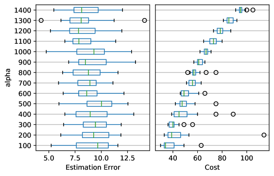
Figure 2: Effect of varying the $\operatorname{ESS}_{\text{min}}$ parameter ($y$-axis) defining the minimum ESS to be reached for calibration of the interse temperature. As stopping depends on the total estimated ESS, the MSE of the variance ($x$-axis on the left) estimation doesn’t depend on $\operatorname{ESS}_{\text{min}}$, but the number of required iterations ($x$-axis on the right) before convergence of the sequence of proposal distributions increases. Increasing $\operatorname{ESS}_{\text{min}}$ further than the minimum required to stabilize the calibration of the new proposal (i.e., of $\theta_{t+1})$ with the EM step results in an increased computational cost.

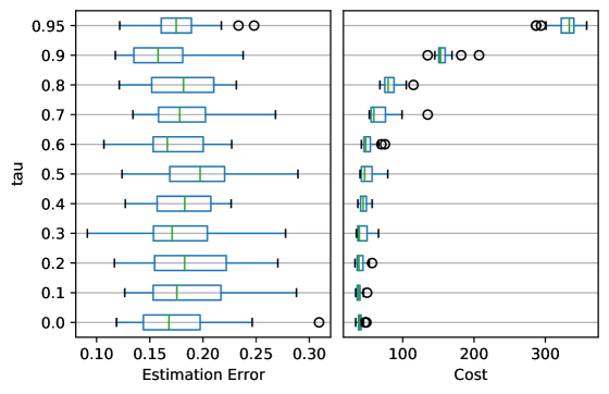
Figure 3: Effect of varying the $\tau$ parameter ($y$-axis) defining the antitruncation threshold. Except for very high values, the truncation has no detrimental effect on either the MSE ($x$-axis on the left) of the estimated variance or the required number of iterations ($x$-axis on the right) before convergence of the sequence of proposal distributions increases. As for $\operatorname{ESS}_{\text{min}}$, once the calibration of of the new proposal (i.e., of $\theta_{t+1})$ with the EM step is stable, increasing $\tau$ further only increases the computational cost.

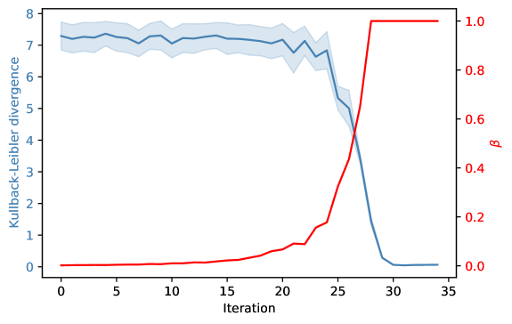
Figure 4: Typical evolution of the inverse temperature $\beta$ ($y$-axis in red) and estimated Kullback-Leibler divergence ($y$-axis in blue) along iterations ($x$-axis). The automatically calibrated $\beta$ starts by increasing slowly until a sharp acceleration, followed by stabilization clearly indicating convergence of sequence of proposal distributions. The estimated KL divergence shows the upper bound biais until iteration $20$, as detailed in 3.2. Yet its sharp decrease and stabilization mirrors $\beta$’s path.

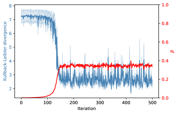
Figure 5: A very high-dimensional problem : The target is a $1000$-dimensional gaussian distribution, the proposals are gaussian distributions with diagonal covariance. (left) Evolution of the inverse temperature $\beta$ (in red) and estimated Kullback-Leibler divergence (blue) along iterations. (right) the L2 distance between the moments of the target and proposal distribution at each iteration. The temperature doesn’t go to $1$ despite the target distribution belonging to the family of proposal distributions and the covariance of the proposal doesn’t converge to the real covariance.

4 Numerical Experiments

We finally illustrate the good numerical properties of TAMIS relatively to its initialization and to the dimensionality of the problem.

Table 2: Initialization and dimensionality

Experiment	E4.1	E4.2	E4.3
Dimension	$d\in\{20,50\}$	$d\in\{5,10,20,50,100\}$	$d\in\{300,500\}$
Target	Rosenbrock distr.	$\mathcal{N}(50,5)^{\otimes d}$
Proposal	Gaussian mixture with 5 components
Draws	$N_{t}=2,000$	$N_{t}=1,000$	$N_{t}=2,000$
$\textbf{ESS}_{\textbf{min}}$	$100$	$300$	$1,000$
$\boldsymbol{\tau}$	$0.4$
Stop	$t=20$	$\sum_{t}\operatorname{ESS}_{t}>1,000$

4.1 On the effect of initialization

We now compare the effect of a bad initialization on TAMIS, AMIS and N-PMC with Experiment E4.1 given in Table 2. The example considered is the banana shape target density of Haario et al., also know as the Rosenbrock distribution. Let $\sigma^{2}=100,\Sigma=\text{diag}(\sigma^{2},1,\dots,1),b=0.03$ and $\Psi(x)=\left(x_{1},x_{2}+b(x_{1}^{2}-\sigma^{2}),x_{3},\dots,x_{d}\right)$. The target is the Rosebrock distribution with density

$$\pi(x)=\varphi(\Psi(x)|0,\Sigma).$$

For N-PMC, the inverse temperature sequence is chosen as in [10], i.e., $\beta_{t}=1/(1+e^{-(t-\ell)})$ where $\ell$ is a tuning parameter we have set to $5$.

The first proposal at initialization is a Gaussian mixture model with 5 components with covariance matrix all equal to $\Sigma$, and centered at random $\mu_{k}$ drawn from $\mathcal{N}(0,\Sigma_{0,k}/5)$. We used various covariance matrices $\Sigma$, starting from the diagonal matrix $\mathrm{diag}(200,50,4,\dots,4)$ used in [20] and [10]. This initial covariance matrix is already adapted to the target and can be considered as an a priori informed proposal. Then, we used less informed covariance matrices for $\Sigma$:

• $\mathrm{diag}(200,50,10,\dots,10)$,

• $\mathrm{diag}(200,50,20,\dots,20)$, $\mathrm{diag}(200,50,50,\dots,50)$,

• $\mathrm{diag}(200,100,100,\dots,100)$ and

• finally $200\times\mathrm{I}_{d}$ which is blind regarding the shape of the target.

Each experiment was repeated $500$ times.

Figure 6 shows the final ESS. As expected the final ESS after a fixed number of iterations decreases as the initialization gets worse. Since the dimension is already high, AMIS fails very frequently even with the first initialization. The tempering scheme of N-PMC is effective only with a well calibrated initialization, while TAMIS remains effective and allows the algorithm to converge in every case without any additional parameter tuning.

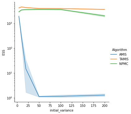
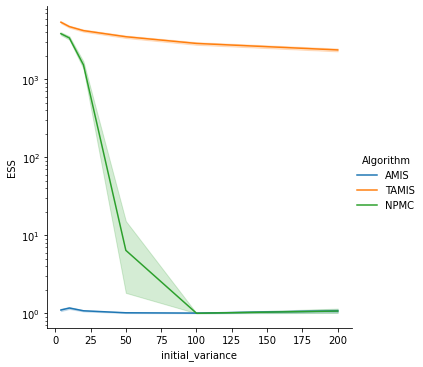
Figure 6: Effective Sample Size ($y$-axis) of AMIS, N-PMC and TAMIS after $40,000$ draws along 20 iterations, with increasingly wide covariance matrix at initialization ($x$-axis) in dimension 20 (left) and 50 (right). As expected from the litterature, AMIS is only performing well with a good initialization and if the dimension is relatively low. N-PMC is able to correct for bad initialization with a well chosen tempering path if the dimension is low enough, while TAMIS performs well in every case.

4.2 On the effect of dimensionality

We now consider a simple Gaussian target

$$\mathcal{N}(50,5)^{\otimes d}$$

of Experiment E4.3 of Table 2 in high dimension. We only consider TAMIS only, as both AMIS and N-PMC fail in every case. The initialization of the proposal distribution is poor for both location and for scale. The proposal distributions are Gaussian mixture models with $5$ components. At initialization, they are centered at random $\mu_{k}\sim\text{Unif}([-4,4])^{\otimes d}$ and have covariance matrices $\Sigma_{k}=200\times\mathrm{I}_{d}$. The target is therefore very concentrated and centered very far in the tail of the initial proposal. The other tuning details are given in Table 2.

We plot the MSE when estimating the trace of the covariance matrix along iterations. We also plot the number of likelihood evaluations required before convergence of the proposal (assessed by the number of iterations such that $\hat{\mathrm{KL}}(\pi||q_{t})>1$ in Figure 7.

The number of simulations required before convergence increases as expected with the dimension. But we note that not only is TAMIS able to accurately estimate scale and location of a very high dimensional target, it does so with the same bad initialization as previously, with very little tuning required.

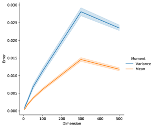
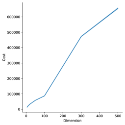
Figure 7: Mean square error ($y$-axis on the left) of the estimates of the mean and covariance for increasing dimension ($x$-axis) and the required number of iterations ($y$-axis on the right) before convergence of the proposal to the target distribution (right).

5 Conclusion

We have designed an adaptive importance sampling that is

• robust to poor initialization of proposal and

• robust to high dimension of the space to sample

• efficient in the number of evaluations of the target density and

• does not rely on any gradient computation.

Very few importance sampling algorithm are stable in dimension higher than $100$, and TAMIS is one of them. Therefore, TAMIS can be used to initialize other Monte Carlo algorithm such as MCMC methods that can lead to more precise estimates when correctly initialized. The phase transition observed in the decrease of the Kullbuck-Leibler divergence we monitor remains to be explained theoretically.

Appendix A Results on the tempered targets

Here, we consider that $\pi(x)$ and $q_{t}(x)$ are normalized densities.

For all $\beta\in[0;1]$, we introduce the normalized density

$$\pi_{\beta,t}(x) =\frac{1}{C_{t}(\beta)}\pi^{\beta}(x)q_{t}^{1-\beta}(x)\quad\text{where }C_{t}(\beta)=\int\pi^{\beta}(x)q_{t}^{1-\beta}(x)\mathrm{d}x.$$

Since the logarithm is a concave function, we have for all $\beta$ and $x$,

$$\pi^{\beta}(x)q_{t}^{1-\beta}(x)\leq\beta\pi(x)+(1-\beta)q_{t}(x).$$

Thus, for all $\beta$, $C_{t}(\beta)\leq 1$. Moreover, $C_{t}(0)=C_{t}(1)=1$.

Proposition 3.

The function $\beta\mapsto\operatorname{KL}(\pi\|\pi_{\beta,t})$ is a convex, non increasing function. It decreases from $\operatorname{KL}(\pi|q_{t})$ to $0$.

Proof of Proposition 3.

Set for all $\beta$, $k(\beta)=\operatorname{KL}(\pi\|\pi_{\beta,t})$. We have

$$k(\beta) =\int\pi(x)\log\frac{\pi(x)C_{t}(\beta)}{\pi^{\beta}(x)q_{t}^{1-\beta}(x)}\mathrm{d}x=(1-\beta)\operatorname{KL}(\pi\|q_{t})+\log C_{t}(\beta).$$

Hence its first and second derivatives are

$$k^{\prime}(\beta)=-\operatorname{KL}(\pi\|q_{t})+\frac{C^{\prime}_{t}(\beta)}{C_{t}(\beta)},\quad k^{\prime\prime}(\beta)=\frac{C^{\prime\prime}_{t}(\beta)}{C_{t}(\beta)}-\left(\frac{C^{\prime}_{t}(\beta)}{C_{t}(\beta)}\right)^{2}.$$ (8)

On the other hand, the first and second derivative of $C_{t}(\beta)$ are

$$C^{\prime}_{t}(\beta) =\int\pi^{\beta}(x)q_{t}^{1-\beta}(x)\log\frac{\pi(x)}{q_{t}(x)}\mathrm{d}x=C_{t}(\beta)\,\mathbb{E}_{\beta,t}\left(\log\frac{\pi(x)}{q_{t}(x)}\right),$$

$$C^{\prime\prime}_{t}(\beta) =\int\pi^{\beta}(x)q_{t}^{1-\beta}(x)\log^{2}\frac{\pi(x)}{q_{t}(x)}\mathrm{d}x=C_{t}(\beta)\,\mathbb{E}_{\beta,t}\left(\log^{2}\frac{\pi(x)}{q_{t}(x)}\right).$$

where $\mathbb{E}_{\beta,t}$ is the expected value when $x\sim\pi_{\beta,t}(x)$. Thus, using (8),

$$k^{\prime\prime}(\beta)=\text{Var}_{\beta,t}\left(\log\frac{\pi(x)}{q_{t}(x)}\right)\geq 0$$

and $k(\beta)$ is a convex function.

Moreover, using (8) again, we have

$$k^{\prime}(1)=-\operatorname{KL}(\pi\|q_{t})+\frac{C^{\prime}_{t}(1)}{C_{t}(1)}=-\operatorname{KL}(\pi\|q_{t})+\int\pi(x)\log\frac{\pi(x)}{q_{t}(x)}\mathrm{d}x=0.$$

Because of the convexity of $k$, for all $\beta\in[0,1]$, $k^{\prime}(\beta)\leq k^{\prime}(1)=0$. Thus, $k(\beta)$ is decreasing and the proof is completed. ∎

The proposition given below is similar to the one of [2], but the proof we give here deals with finite samples.

Proposition 4.

Consider a collection of positive weights $w_{i}$, $i=1,\ldots,n$. The function $\beta\mapsto\operatorname{ESS}(\beta)$ defined by

$$\operatorname{ESS}(\beta)=\left(\sum_{i=1}^{n}w_{i}^{\beta}\right)^{2}\Big{/}\left(\sum_{i=1}^{n}w_{i}^{2\beta}\right)$$

is decreasing.

Proof.

If $x>0$, the derivate of $x^{\beta}$ with respect to $\beta$ is $x^{\beta}\log x$. Hence,

$$\frac{\mathrm{d}}{\mathrm{d}\beta}\operatorname{ESS}(\beta) =\frac{\displaystyle 2g(\beta)\sum_{i=1}^{n}w_{i}^{\beta}}{\displaystyle\left(\sum_{i=1}^{n}w_{i}^{2\beta}\right)^{2}}\quad\text{where}$$

$$g(\beta) =\left(\sum_{i=1}^{n}w_{i}^{\beta}\log w_{j}\right)\sum_{j=1}^{n}w_{j}^{2\beta}-\left(\sum_{j=1}^{n}w_{j}^{2\beta}\log w_{i}\right)\sum_{i=1}^{n}w_{i}^{\beta}.$$

Now,

$$g(\beta) =\sum_{1\leq i,j\leq n}w_{i}^{2\beta}w_{j}^{\beta}\Big{(}\log w_{j}-\log w_{i}\Big{)}$$

$$=\sum_{1\leq i<j\leq n}w_{i}^{\beta}w_{j}^{\beta}\Big{(}\log w_{j}-\log w_{i}\Big{)}\Big{(}w_{i}^{\beta}-w_{j}^{\beta}\Big{)}$$

$$\leq 0,$$

since, for all $a,b>0$,

$$a^{2\beta}b^{\beta}(\log b-\log a)+a^{\beta}b^{2\beta}(\log a-\log b)=a^{\beta}b^{\beta}\Big{(}a^{\beta}-b^{\beta}\Big{)}\log\frac{b}{a}\leq 0.\qed$$

Appendix B Proof of Proposition 2

We start with this simple Lemma.

Lemma 5.

Let $f(x)$ and $g(x)$ be two densities on the $x$-space, which partitioned by $E\cup\bar{E}$. Introduce the normalized densities knowing $x\in E$ or $\bar{E}$ as

$$f_{|E}(x)=\frac{1}{f(E)}f(x)\mathbf{1}_{E}(x),\quad f_{|\bar{E}}(x)=\frac{1}{f(\bar{E})}f(x)\mathbf{1}_{\bar{E}}(x)$$

and likewise for $g_{|E}$ and $g_{|\bar{E}}$. We have

$$\operatorname{KL}\big{(}f\big{\|}g\big{)}=f(E)\,\operatorname{KL}\big{(}f_{|E}\big{\|}g_{|E}\big{)}+f(\bar{E})\,\operatorname{KL}\big{(}f_{|\bar{E}}\big{\|}g_{|\bar{E}}\big{)}+f(E)\log\frac{f(E)}{g(E)}+f(\bar{E})\log\frac{f(\bar{E})}{g(\bar{E})}.$$

Proof.

We have

$$\operatorname{KL}\big{(}f\big{\|}g\big{)}=\int_{E}f(x)\log\frac{f(x)}{g(x)}\mathrm{d}x+\int_{\bar{E}}f(x)\log\frac{f(x)}{g(x)}\mathrm{d}x.$$

Moreover

$$\int_{E}f(x)\log\frac{f(x)}{g(x)}\mathrm{d}x =\int_{E}f(E)f_{|E}(x)\log\frac{f(E)f_{|E}(x)}{g(E)g_{|E}(x)}\mathrm{d}x$$

$$=f(E)\int_{E}f_{|E}(x)\log\frac{f_{|E}(x)}{g_{|E}(x)}\mathrm{d}x+f(E)\log\frac{f(E)}{g(E)}$$

$$=f(E)\,\operatorname{KL}\big{(}f_{|E}\big{\|}g_{|E}\big{)}+f(E)\log\frac{f(E)}{g(E)}.$$

Likewise,

$$\int_{\bar{E}}f(x)\log\frac{f(x)}{g(x)}\mathrm{d}x =f(\bar{E})\,\operatorname{KL}\big{(}f_{|\bar{E}}\big{\|}g_{|\bar{E}}\big{)}+f(\bar{E})\log\frac{f(\bar{E})}{g(\bar{E})}.\qed$$

Proof of Propostion 2.

Using Lemma 5, $\operatorname{KL}\Big{(}\pi_{\beta,t}\Big{\|}\widehat{\pi}_{\beta,t}\Big{)}=\operatorname{KL}_{I}+\operatorname{KL}_{II}+\operatorname{KL}_{III}$ where

$$\operatorname{KL}_{I} =\pi_{\beta,t}(E)\operatorname{KL}\Big{(}\pi_{\beta,t}^{E}\Big{\|}q_{t}^{E}\Big{)}$$

$$\operatorname{KL}_{II} =\pi_{\beta,t}(\bar{E})\operatorname{KL}\Big{(}\pi_{\beta,t}^{\bar{E}}\Big{\|}\pi_{\beta,t}^{\bar{E}}\Big{)}=0$$

$$\operatorname{KL}_{III} =\pi_{\beta,t}(E)\log\frac{\pi_{\beta,t}(E)}{\lambda}+(1-\pi_{\beta,t}(E))\log\frac{1-\pi_{\beta,t}(E)}{1-\lambda}.$$

Likewise, $\operatorname{KL}\Big{(}\pi_{\beta,t}\Big{\|}q_{t}\Big{)}=\operatorname{KL}_{I}^{\prime}+\operatorname{KL}_{II}^{\prime}+\operatorname{KL}_{III}^{\prime}$ where

$$\operatorname{KL}_{I}^{\prime} =\pi_{\beta,t}(E)\operatorname{KL}\Big{(}\pi_{\beta,t}^{E}\Big{\|}q_{t}^{E}\Big{)}=\operatorname{KL}_{I}$$

$$\operatorname{KL}_{II}^{\prime} =\pi_{\beta,t}(\bar{E})\operatorname{KL}\Big{(}\pi_{\beta,t}^{\bar{E}}\Big{\|}q_{t}^{\bar{E}}\Big{)}\geq 0=\operatorname{KL}_{II}$$

$$\operatorname{KL}_{III}^{\prime} =\pi_{\beta,t}(E)\log\frac{\pi_{\beta,t}(E)}{q_{t}(E)}+(1-\pi_{\beta,t}(E))\log\frac{1-\pi_{\beta,t}(E)}{1-q_{t}(E)}.$$

Moreover, when $s\leq 1$, $\lambda=sq_{t}(E)\leq q_{t}(E)$, thus $\operatorname{KL}_{III}^{\prime}\geq\operatorname{KL}_{III}$. Finally,

$$\operatorname{KL}\Big{(}\pi_{\beta,t}\Big{\|}\widehat{\pi}_{\beta,t}\Big{)}=\operatorname{KL}_{I}+\operatorname{KL}_{II}+\operatorname{KL}_{III}\leq\operatorname{KL}_{I}^{\prime}+\operatorname{KL}_{II}^{\prime}+\operatorname{KL}_{III}^{\prime}=\operatorname{KL}\Big{(}\pi_{\beta,t}\Big{\|}q_{t}\Big{)}.\qed$$

References

- Beaujean and Caldwell, [2013] Beaujean, F. and Caldwell, A. (2013). Initializing adaptive importance sampling with markov chains.
- Beskos et al., [2016] Beskos, A., Jasra, A., Kantas, N., and Thiery, A. (2016). On the convergence of adaptive sequential Monte Carlo methods. The Annals of Applied Probability, 26(2):1111 – 1146.
- Bugallo et al., [2017] Bugallo, M. F., Elvira, V., Martino, L., Luengo, D., Miguez, J., and Djuric, P. M. (2017). Adaptive importance sampling: The past, the present, and the future. IEEE Signal Processing Magazine, 34(4):60–79.
- Cappé et al., [2008] Cappé, O., Douc, R., Guillin, A., Marin, J.-M., and Robert, C. P. (2008). Adaptive importance sampling in general mixture classes. Statistics and Computing, 18(4):447–459.
- Cornuet et al., [2012] Cornuet, J.-M., Marin, J.-M., Mira, A., and Robert, C. P. (2012). Adaptive multiple importance sampling. Scandinavian Journal of Statistics, 39(4):798–812.
- Delyon and Portier, [2021] Delyon, B. and Portier, F. (2021). Safe adaptive importance sampling: A mixture approach. The Annals of Statistics, 49(2):885 – 917.
- El-Laham et al., [2018] El-Laham, Y., Elvira, V., and Bugallo, M. (2018). Robust Covariance Adaptation in Adaptive Importance Sampling. IEEE Signal Processing Letters, 25(7):1049–1053.
- Fruhwirth-Schnatter et al., [2019] Fruhwirth-Schnatter, S., Celeux, G., and Robert, C. P. (2019). Handbook of mixture analysis. CRC press.
- Ionides, [2008] Ionides, E. L. (2008). Truncated importance sampling. Journal of Computational and Graphical Statistics, 17(2):295–311.
- Koblents and Míguez, [2015] Koblents, E. and Míguez, J. (2015). A population monte carlo scheme with transformed weights and its application to stochastic kinetic models. Statistics and Computing, 25(2):407–425.
- Korba and Portier, [2022] Korba, A. and Portier, F. (2022). Adaptive importance sampling meets mirror descent : a bias-variance tradeoff. In Camps-Valls, G., Ruiz, F. J. R., and Valera, I., editors, Proceedings of The 25th International Conference on Artificial Intelligence and Statistics, volume 151 of Proceedings of Machine Learning Research, pages 11503–11527. PMLR.
- Liu, [2001] Liu, J. S. (2001). Monte Carlo strategies in scientific computing, volume 10. Springer.
- Marin et al., [2019] Marin, J.-M., Pudlo, P., and Sedki, M. (2019). Consistency of adaptive importance sampling and recycling schemes. Bernoulli, 25(3):1977–1998.
- Neal, [2001] Neal, R. M. (2001). Annealed importance sampling. Statistics and Computing, 11(22):125–139.
- Oh and Berger, [1992] Oh, M.-S. and Berger, J. O. (1992). Adaptive importance sampling in monte carlo integration. Journal of Statistical Computation and Simulation, 41(3-4):143–168.
- Oh and Berger, [1993] Oh, M.-S. and Berger, J. O. (1993). Integration of multimodal functions by monte carlo importance sampling. Journal of the American Statistical Association, 88(422):450–456.
- Owen and Zhou, [2000] Owen, A. and Zhou, Y. (2000). Safe and effective importance sampling. Journal of the American Statistical Association, 95(449):135–143.
- Robert et al., [1999] Robert, C. P., Casella, G., and Casella, G. (1999). Monte Carlo statistical methods, volume 2. Springer.
- Vehtari et al., [2021] Vehtari, A., Simpson, D., Gelman, A., Yao, Y., and Gabry, J. (2021). Pareto smoothed importance sampling.
- Wraith et al., [2009] Wraith, D., Kilbinger, M., Benabed, K., Cappé, O., Cardoso, J.-F. m. c., Fort, G., Prunet, S., and Robert, C. P. (2009). Estimation of cosmological parameters using adaptive importance sampling. Phys. Rev. D, 80:023507.