On The Uncertainty Principle of Neural Networks

Abstract

Despite the successes in many fields, it is found that neural networks are difficult to be both accurate and robust, i.e., high accuracy networks are often vulnerable. Various empirical and analytic studies have substantiated that there is more or less a trade-off between the accuracy and robustness of neural networks. If the property is inherent, applications based on the neural networks are vulnerable with untrustworthy predictions. To more deeply explore and understand this issue, in this study we show that the accuracy-robustness trade-off is an intrinsic property whose underlying mechanism is closely related to the uncertainty principle in quantum mechanics. By relating the loss function in neural networks to the wave function in quantum mechanics, we show that the inputs and their conjugates cannot be resolved by a neural network simultaneously. This work thus provides an insightful explanation for the inevitability of the accuracy-robustness dilemma for general deep networks from an entirely new perspective, and furthermore, reveals a potential possibility to study various properties of neural networks with the mature mathematical tools in quantum physics.

1 Introduction

1.1 Background

An intriguing issue concerning the deep neural networks has garnered significant attentions recently. Despite wide applications in many fields, such as image classification[1], speech recognition[2], playing chess[3] and games[4], predicting protein structures[5], designing chips[6], searching for particles[7], and solving quantum systems[8, 9], etc., these well-trained models are found to be vulnerable under attacks that are imperceptible in terms of human sensations. Overwhelming empirical evidences have manifested that a small non-random perturbation can make a carefully designed neural network give erroneous predictions at a high coincidence[10, 11, 12, 13, 14, 15, 16, 17].

Seeing the fact that more and more researchers are seeking to understand the neural networks, it is crucial for us to further study the accuracy-robustness trade-off of these networks as aforementioned. Meanwhile, since many researchers are using neural networks in their investigations, it is also important for us to explore that if the neural networks are brittle to even small perturbations, which might potentially make applications based on the state-of-the-art deep learning under potential risks. For instance, catastrophic accident may occur on self-driving cars if any inperceptable noises are added on the road signs; medical diagnose can falsely discriminate the cancer cells due to disturbances that the doctors cannot tell by eyes; and personal bank account based on face recognition may be crashed when hacked by small negligible pixels, etc.

To understand the phenomenon, various empirical studies[18, 15, 19] involving different network structures, sizes, performances and even the scales of the training data, do substantiate that there is more or less a trade-off between the accuracy and the robustness of a general neural network. Along with the experimental evidences, theoretical studies[20, 21, 22, 23], ranging from binary classification models to the information theory based analysis, also support the possibility of such trade-off in neural networks. Despite the fact that we still lack a proof to certify these phenomena, many researchers have already begun the concurrent training strategy which optimizes both the robustness and the accuracy of deep neural networks[24, 25, 19, 22, 26, 27, 28, 29].

1.2 Motivation

To the best of our knowledge, the underlying theoretical reason for this accuracy-robustness trade-off is still unknown so far, and it is still not sure whether we can ultimately invent a neural network with both sufficient accuracy and robustness. Therefore, it is of vital importance to clarify the issue, in hope to make all future man-made products relying on the neural networks possibly be predictable and controllable.

Intuitively, it is hard to understand the vulnerability phenomenon since the classical approximation theorems have already shown that a continuous function can be approximated arbitrarily well by a neural network[30, 31, 32, 33]. That is, stable problems described by stable functions should always be solved stably in principle. Therefore, a natural question concerning this issue is to ask whether this accuracy-robustness trade-off is an intrinsic and universal property possessed by general neural networks. If it is purely a matter of neural architecture design and training data acquisition, it is then only needed to concentrate on the designing and training perspectives. If, otherwise, it involves some intrinsic properties which stand at the foundations of deep learning, it is then crucial to further study this trade-off issue in depth.

1.3 Contribution of this work

In this work, we theoretically show that the accuracy-robustness trade-off of a neural network can be insightfully understood under the uncertainty principle in quantum mechanics, where two complementary factors cannot be measured to an arbitrary high accuracy simultaneously (see derivation in Sec. 3). In terms of neural networks, the uncertainty principle implies that one cannot expect a trained neural network to extract two complementary features of a same input to an arbitrary accuracy. For example, in image classification, if one has trained a network with high accuracy on distinguishing an image class (e.g., dog), this class samples tend to be more easily attacked to enter the domain of other distinguished classes (e.g.,car,deer,etc.).

To verify the above statement, we list various experimental evidences both from our attempts and other literatures in Sec. 4. Many experiments with different network structures, datasets, attack strengths as well as loss functions all suggest the inevitable uncertainty principle for general neural networks.

Specifically, our work reveals that neural networks obey the complementarity principle[34] and cannot be both extremely accurate and robust. If we can find out the complementary features of a neural network, we will be able to conduct a concurrent training[25] to possibly achieve a better balance between the accuracy and robustness in the specific applications. Moreover, by introducing the mature mathematics, which has been developed for over 100 years in physics, to the neural networks, we have demonstrated the potential possibility to analyze more intrinsic properties of neural networks in terms of quantum physics.

2 Relevant information

For the convenience of introducing our main theoretical result, in this section we present some relevant information. Firstly, we introduce one of the most classical and simplest attacking methods, the FGSM attack, as an typical instance to intuitively demonstrate the attacking effect on neural networks. Then, we introduce the necessary knowledge on the uncertainty principle in quantum physics.

2.1 The FGSM attack

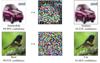
Figure 1: FGSM attack reduces the test accuracy by adding an imperceptible non-random noise. The trained Googlenet on Cifar-10[35] (see the architecture and implementation in Ref. [36]) gives a 90.78% test accuracy on the test set and only 3.67% robust accuracy under the FGSM attack. The attack is achieved via the transformation $X=X_{0}+\epsilon\cdot\text{sign}(\nabla_{X}l(f(X,\theta),Y^{*})|_{X=X_{0}})$, where $X_{\text{0}}$ denotes the input images of the training set and $X$ denotes the image to be attacked, $\epsilon=8/255$ and $\text{sign}(\nabla_{X}l(f(X,\theta),Y^{*})|_{X=X_{0}})$ gives the non-random noise with $l(f(X,\theta),Y^{*})$ denoting the loss function. $\theta$ denotes the weights of the trained network.

One of the most classical and simplest attacking methods is the Fast Gradient Sign Method[21] (FGSM) presented by Goodfellow et al. in 2015. Given a loss function $l(f(X,\theta),Y^{*})$, the FGSM creates an attack $X$ by

$$X = X_{0}+\epsilon\cdot\text{sign}(\nabla_{X}l(f(X,\theta),Y^{*})|_{X=X_{0}}),$$ (1)

where the loss function $l$ is obtained under a network model $f(X,\theta)$ with parameters $\theta$ trained on a pre-collected training dataset, and $\epsilon$ is a positive number usually taken to be a small value to make the attack possibly imperceptible. $X_{0}$ denotes the raw image to be attacked and classified, and $Y^{*}$ is the true label for image $X_{0}$. Here, $\nabla_{X}l(f(X,\theta),Y^{*})$ is interpreted as the gradient of $l$ with respect to $X$. For most of the classifiers, the loss function $l$ is simply the training loss used in training the network. Note that the choice of the loss function does not significantly affect the performance of the attack [37, 38]. Since the gradient is not difficult to compute for deep neural networks, the attack can always be efficiently implemented.

Fig. 1 depicts the effect of the FGSM attack on two typical images of the Cifar-10 dataset. The trained network correctly identifies the “red car” ($X_{0}$ in Eq. (1)) in the left panel as Automobile with a 99.99% confidence, but falsely classifies the attacked one ($X$ in Eq. (1)) on the right panel as Airplane with a 54.53% confidence. Since the two images $X_{0}$ and $X$ are imperceptable in terms of human eyes, it is interesting to ask why the neural network fails at identifying them.

2.2 Uncertainty principle in quantum physics

In this subsection, all physical quantities are expressed in the natural unit. In quantum physics, we can describe a particle by a wave packet $\psi(X)$ in the coordinate representation with respect to the coordinate reference frame. The normailzation condition for $\psi(X)$ is given by

$$\int|\psi(X)|^{2}dX = 1,$$ (2)

where the square amplitude $|\psi(X)|^{2}$ gives the probability density for finding a particle at position $X=(x,y,z)$. To measure the physical quantities of the particle, such as position $X$ and momentum $P=(p_{x},p_{y},p_{z})$, we need to define the position and momentum operators $\hat{x}_{i}$ and $\hat{p}_{i}$ as:

$$\hat{x}_{i}\psi(X) = x_{i}\psi(X),$$

$$\hat{p}_{i}\psi(X) = -i\frac{\partial}{\partial x_{i}}\psi(X),$$ (3)

where $i=1,2,3$ denote the $x,y,z$ components in the coordinate space, respectively. The average position and momentum of the particle can be evaluated by

$$\langle\hat{x}_{i}\rangle = \int\psi^{*}(X)x_{i}\psi(X)dX$$

$$\langle\hat{p}_{i}\rangle = \int\psi^{*}(X)[-i\frac{\partial}{\partial x_{i}}\psi(X)]dX,$$ (4)

where $\langle\cdot\rangle$ is the Dirac symbol widely used in physics and $\psi^{*}(X)$ is the complex conjugate of $\psi(X)$. The standard deviations of the position $\sigma_{x_{i}}$ and momentum $\sigma_{p_{i}}$ are defined respectively as:

$$\sigma_{x_{i}} = \langle(\hat{x}_{i}-\langle\hat{x}_{i}\rangle)^{2}\rangle^{1/2},$$

$$\sigma_{p_{i}} = \langle(\hat{p}_{i}-\langle\hat{p}_{i}\rangle)^{2}\rangle^{1/2}.$$ (5)

In the year of 1927, Heisenberg introduced the first formulation of the uncertainty principle in his German article[39]. The Heisenberg’s uncertainty principle asserts a fundamental limit to the accuracy for certain pairs. Such variable pairs are known as complementary variables (or canonically conjugate variables). The formal inequality relating the standard deviation of position $\sigma_{x_{i}}$ and the standard deviation of momentum $\sigma_{p_{i}}$ reads

$$\sigma_{x_{i}}\sigma_{p_{i}} \geq \frac{1}{2}.$$ (6)

Uncertainty relation Eq. (6) states a fundamental property of quantum systems and can be understood in terms of the Niels Bohr’s complementarity principle[34]. That is, objects have certain pairs of complementary properties cannot be observed or measured simultaneously.

3 Uncertainty principle for neural networks

3.1 Formulas and notations for neural networks

Without loss of generality, we can assume that the loss function $l(f(X,\theta),Y)$ is square integrable,

$$\int l(f(X,\theta),Y)^{2}dX = \beta.$$ (7)

Eq. (7) allows us to further normalize the loss function as

$$\psi_{Y}(X) = \frac{l(f(X,\theta),Y)}{\beta^{1/2}},$$ (8)

so that

$$\int\psi_{Y}(X)^{2}dX=1.$$ (9)

For convenience, we refer $\psi_{Y}(X)$ as a neural packet in the later discussions. Note that under different labels $Y$, a neural network will be with a set of neural packets.

An image $X=(x_{1},...,x_{i},...,x_{M})$ with $M$ pixels can be seen as a point in the multi-dimensional space, where the numerical values of $(x_{1},...,x_{i},...,x_{M})$ correspond to the pixel values. The pixel and attack operators of the neural packet $\psi_{Y}(X)$ can then be defined as:

$$\hat{x}_{i}\psi_{Y}(X) = x_{i}\psi_{Y}(X),$$

$$\hat{p}_{i}\psi_{Y}(X) = \frac{\partial}{\partial x_{i}}\psi_{Y}(X).$$ (10)

Similar as Eq. (4), the average pixel value at $x_{i}$ associated with neural packet $\psi_{Y}(X)$ can be evaluated as

$$\langle\hat{x}_{i}\rangle = \int\psi_{Y}^{*}(X)x_{i}\psi_{Y}(X))dX.$$ (11)

Since $\psi_{Y}(X)$ corresponds to a purely real number without imaginary part, the above equation is equivalent to:

$$\langle\hat{x}_{i}\rangle = \int\psi_{Y}(X)x_{i}\psi_{Y}(X))dX.$$ (12)

Besides, the attack operator $\hat{p}_{i}=\frac{\partial}{\partial x_{i}}$ corresponds to the conjugate variable of $x_{i}$. And we can obtain the average value for $\hat{p_{i}}$ as

$$\langle\hat{p}_{i}\rangle = \int\psi_{Y}(X)\frac{\partial}{\partial x_{i}}\psi_{Y}(X)dX.$$ (13)

3.2 Derivation of the uncertainty relation

TABLE I: Comparison of the uncertainty principle between quantum physics and neural networks.

Quantum physics		Neural networks
position	$X=(x,y,z)$	$X=(x_{1},...,x_{i},...,x_{M})$	image (input)
momentum (conjugate of position)	$P=(p_{x},p_{y},p_{z})$	$P=(p_{1},...,p_{i},...,p_{M})$	attack (conjugate of input)
wave function	$\psi(X)$	$\psi_{Y}(X)$	normalized loss function (neural packet)
normalize condition	$\int|\psi(X)|^{2}dX=1$	$\int|\psi_{Y}(X)|^{2}=1$	normalize condition
position operator	$\hat{x}_{i}\psi(X)=x_{i}\psi(X)$	$\hat{x}_{i}\psi_{Y}(X)=x_{i}\psi_{Y}(X)$	pixel operator
momentum operator	$\hat{p}_{i}\psi(X)=-i\frac{\partial}{\partial x_{i}}\psi(X)$	$\hat{p}_{i}\psi_{Y}(X)=\frac{\partial}{\partial x_{i}}\psi_{Y}(X)$	attack operator
standard deviation for measuring position	$\sigma_{x_{i}}=\langle(\hat{x}_{i}-\langle\hat{x}_{i}\rangle)^{2}\rangle^{1/2}$	$\sigma_{x_{i}}=\langle(\hat{x}_{i}-\langle\hat{x}_{i}\rangle)^{2}\rangle^{1/2}$	standard deviation for resolving pixel
standard deviation for measuring momentum	$\sigma_{p_{i}}=\langle(\hat{p}_{i}-\langle\hat{p}_{i}\rangle)^{2}\rangle^{1/2}$	$\sigma_{p_{i}}=\langle(\hat{p}_{i}-\langle\hat{p}_{i}\rangle)^{2}\rangle^{1/2}$	standard deviation for resolving attack
uncertainty relation	$\sigma_{x_{i}}\sigma_{p_{i}}\geq\frac{1}{2}$	$\sigma_{x_{i}}\sigma_{p_{i}}\geq\frac{1}{2}$	uncertainty relation

The uncertainty principle of a trained neural network can then be deduced by the following theorem:

Theorem 1.

The standard deviations $\sigma_{{p}_{i}}$ and $\sigma_{{x}_{i}}$ corresponding to the attack and pixel operators $\hat{p_{i}}$ and $\hat{x_{i}}$, respectively, are restricted by the relation:

$$\sigma_{{p}_{i}}\sigma_{{x}_{i}} \geq \frac{1}{2}.$$ (14)

Proof.

We first introduce the standard deviations $\sigma_{a}$ and $\sigma_{b}$ corresponding to two general operators $\hat{A}$ and $\hat{B}$. Then it follows that:

$$\sigma_{a}\sigma_{b}=\langle(\hat{A}-\langle\hat{A}\rangle)^{2}\rangle^{\frac{1}{2}}\langle(\hat{B}-\langle\hat{B}\rangle)^{2}\rangle^{\frac{1}{2}}\equiv\langle\hat{a}^{2}\rangle^{\frac{1}{2}}\langle\hat{b}^{2}\rangle^{\frac{1}{2}}.$$

(15)

In general, for any two unbounded real operators $\langle\hat{a}\rangle$ and $\langle\hat{b}\rangle$, the following relation holds

$$0\leq\langle(\hat{a}-i\hat{b})^{2}\rangle=\langle\hat{a}^{2}\rangle-i\langle\hat{a}\hat{b}-\hat{b}\hat{a}\rangle+\langle\hat{b}^{2}\rangle.$$

(16)

If we further replace $\hat{a}$ and $\hat{b}$ in Eq. (16) by operators $\hat{a}\langle\hat{a}^{2}\rangle^{-1/2}$ and $\hat{b}\langle\hat{b}^{2}\rangle^{-1/2}$, we can then obtain the property $2\langle\hat{a}^{2}\rangle^{1/2}\langle\hat{b}^{2}\rangle{}^{1/2}\geq i\langle\hat{a}\hat{b}-\hat{b}\hat{a}\rangle$, which gives the basic bound for the commutator $[\hat{a},\hat{b}]\equiv\hat{a}\hat{b}-\hat{b}\hat{a}$,

$$\langle\hat{a}^{2}\rangle^{\frac{1}{2}}\langle\hat{b}^{2}\rangle^{\frac{1}{2}} \geq |i\frac{1}{2}\langle[\hat{a},\hat{b}]\rangle|.$$ (17)

Seeing the fact that $[\hat{a},\hat{b}]=[\hat{A},\hat{B}]$, we finally obtain the uncertainty relation

$$\sigma_{a}\sigma_{b} \geq |i\frac{1}{2}\langle[\hat{A},\hat{B}]\rangle|.$$ (18)

In terms of the neural networks, we can simply replace operators $\hat{A}$ and $\hat{B}$ by $\hat{p}_{i}$ and $\hat{x}_{i}$ introduced in Eq. (10), and this leads to

$$\sigma_{{p}_{i}}\sigma_{{x}_{i}} \geq |i\frac{1}{2}\langle[\hat{p}_{i},\hat{x}_{i}]\rangle|=\frac{1}{2},$$ (19)

where we have used the relation

$$[\hat{p}_{i},\hat{x}_{i}]\psi_{Y}(X) = [\hat{p}_{i}\hat{x}_{i}-\hat{x}_{i}\hat{p}_{i}]\psi_{Y}(X)$$ (20)

$$= \frac{\partial}{\partial x_{i}}[x_{i}\psi_{Y}(X)]$$

$$-x_{i}\frac{\partial}{\partial x_{i}}\psi_{Y}(X)$$

$$= \psi_{Y}(X).$$

∎

Note that for a trained neural network, $\psi_{Y}(X)$ depends on the dataset and the structure of the network.

Eq. (19) is a general result for general neural networks (see extension to the generation network in supplementary material). For convenience, we compare the formulas in quantum physics with those used in neural networks in Tab. I to facilitate easy understandings for readers.

3.3 Understanding the uncertainty principle

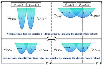
Figure 2: Schematic illustration of the uncertain relation in binary classification. $\psi_{\text{Car}}(X)$ and $\psi_{\text{Deer}}(X)$ denote the normalized loss functions; $\widetilde{\psi}_{\text{Car}}(X)$ and $\widetilde{\psi}_{\text{Deer}}(X)$ denote the corresponding conjugats.

To understand how Eq. (19) leads to the trade-off of accuracy and robustness, we consider an example of a binary classifier which distinguishes two categories, e.g., Car and Deer. In Fig. 2, we schematically plot the neural packets $\psi_{\text{Car}}(X)$ and $\psi_{\text{Deer}}(X)$ in the representation of the pixel variable $X$, as well as their corresponding conjugates. Here the attack operators are denoted as $P=(\hat{p}_{1},...,\hat{p}_{i},...,\hat{p}_{M})$. Images $X$ can be seen as vectors in the high dimensional space. The neural packets map the images into scalar values. The two separated functions in the left panel represent the neural packets of the two classes after training. A higher test accuracy is expected if the standard deviations $\sigma_{X,\text{Car}}$ and $\sigma_{X,\text{Deer}}$ are small, so that the two neural packets can be more easily separated apart (as shown in the upper left panel). In the upper right panel, restricted by the uncertainty relation shown in Eq. (19), $\sigma_{P,\text{Cars}}$ and $\sigma_{P,\text{Deer}}$ are inevitably larger, inclining to more possibly conduct an overlap between the neural packets in $P$. On the other hand, if $\sigma_{X,\text{Cars}}$ and $\sigma_{X,\text{Deer}}$ are relatively larger, the trained network tends to be less accurate, while simultaneously leading to a smaller overlapped region between neural packets in $P$, as illustrated in the lower panel of Fig. 2.

In the FGSM attack, the attacked image is of the form:

$$X = X_{0}+\epsilon\cdot\text{sign}(\nabla_{X}l(f(X,\theta),Y^{*})|_{X=X_{0}})$$ (21)

$$\sim X_{0}+\epsilon\cdot\nabla_{X}l(f(X,\theta),Y^{*})|_{X=X_{0}}$$

$$= X_{0}+\epsilon\cdot\nabla_{X}[\beta^{1/2}\psi_{Y^{*}}(X_{0})]$$

$$= X_{0}+\epsilon^{\prime}\hat{P}\psi_{Y^{*}}(X_{0}),$$

where $\hat{P}=(\frac{\partial}{\partial x_{1}},...,\frac{\partial}{\partial x_{i}},...,\frac{\partial}{\partial x_{M}})$ and $\epsilon^{\prime}=\epsilon\cdot\beta^{1/2}$. In the second line of Eq. (21) we have used the property substantiated in [40]: ”even without the ’Sign’ of the FGSM, a successful attack can also be achieved". From Eq. (21), we can then obtain

$$\hat{P}\psi_{Y^{*}}(X_{0})\sim\epsilon/\epsilon^{\prime}\cdot\text{sign}(\nabla_{X}l(f(X,\theta),Y^{*})|_{X=X_{0}}),$$ (22)

which is the reason that we call $\hat{p_{i}}$ the attack operator. In the upper panel of Fig. 2, we know that the two neural packets tend to overlap in $P$ under small $\sigma_{X,\text{Car}}$ and $\sigma_{X,\text{Deer}}$. Therefore, in such circumstances, a successful attack tends more possibly to occur.

4 Numerical evidences for the uncertainty principle

4.1 Numerical experimental results

To verify the proposed uncertainty principle, we use four different networks, including Convolutional (ConVNet) [41, 42, 43], Residual (ResNet) [44], Google (GoogleNet)[45] and YGCNN [46], as the classifiers. ConvNet, ResNet and GoogleNet are used for Cifar-10 dataset and ConvNet, ResNet and YGCNN are applied on MNIST dataset. The four networks are trained at various epoch numbers $\text{N}_{\text{epoch}}$. Since the network structures are standard, we refer readers to Ref. [36] for more implementation details.

Here the test accuracy (TA) is calculated as the classification accuracy on the test data, and the robust accuracy (RA) is obtained by applying the trained classifiers on the attacked images on the test data. The attack is implemented by employing the Projected Gradient Descent (PDG) method [47, 48], which is considered as one of the most effective ways to achieve moderate adversarial attacks. Inspired by FGSM, PDG performs an iterative attack via

$$X_{\text{n}+1} = \text{Clip}_{\epsilon}\{X_{\text{n}}$$ (23)

$$+\alpha\cdot\text{sign}(\nabla_{X}l(f(X,\theta),Y^{*})|_{X=X_{n}}),$$

where $\text{Clip}_{\epsilon}$ refers to a truncation which limits the data in range $[-\epsilon,\epsilon]$. For the MNIST dataset the attack strength $\alpha$ and clamp bound $\epsilon$ are set to be 0.025 and 0.1, and for Cifar-10 they are specified as $\alpha=2/255$ and $\epsilon=8/255$. All test images are attacked iteratively for 4 steps with $l_{\infty}$ loss.

TABLE II: Test and robust accuracies for different classifiers on MNIST dataset.

Network type	Test accuracy (%)			Robust accuracy (%)
	$\text{N}_{\text{epoch}}$			$\text{N}_{\text{epoch}}$
	1	30	50	1	30	50
ConvNet	97.31	98.71	98.72	41.44	50.98	53.74
ResNet	98.65	99.50	99.57	90.88	98.22	98.27
YGCNN	97.35	99.15	99.19	59.84	49.06	45.68

TABLE III: Test and robust accuracies for different classifiers on Cifar-10 dataset.

Network type	Test accuracy (%)			Robust accuracy (%)
	$\text{N}_{\text{epoch}}$			$\text{N}_{\text{epoch}}$
	1	5	50	1	5	50
ConvNet	45.71	60.46	63.07	12.49	6.62	2.88
ResNet	70.42	82.97	86.86	10.67	14.17	1.45
GoogleNet	67.71	81.18	86.61	10.64	8.44	0.08

Since the uncertainty relation provides a lower bound on the standard deviations, we are able to increase TA and RA simultaneously if the lower bound is not reached. This condition is shown by the result of ConvNet and ResNet in Tab. II (for clarity, we have set these values in bold and italic font), where we present the obtained TA and RA on the MNIST dataset. If the lower bound is approximately reached, as shown by the result of YGCNN, the uncertainty relation will pose a limit on TA and RA. Thus, we see that an increase in TA corresponds to a decrease in RA. Note that higher TA does not necessarily implies that the trained network with neural packet $\psi_{Y^{*}}(X)$ has reached the lower bound. As mentioned in Subsec. 3.2, the neural packet $\psi_{Y^{*}}(X)$ depends on the dataset and the network architecture. Thus, different network structures and datasets may behave differently. This can rationally explain that even though TA for ResNet is larger than that of YGCNN, we can still improve its TA and RA simultaneously. The similar phenomenon can also be observed on Cifar-10 dataset, which can be seen in Tab. III, where an increase in TA corresponds to a decrease in RA.

4.2 Accuracy-robustness trade-off on 18 different deep classification models

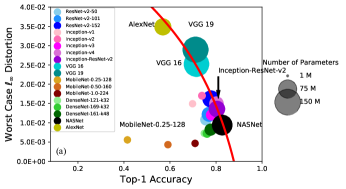
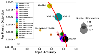
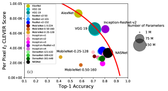
Figure 3: Robustness vs. classification accuracy of I-FGSM attack, $C\&W$ attack and CLEVER score on random targets over 18 ImageNet models. (a) Fitted Pareto frontier of $l_{\infty}$ distortion (I-FGSM attack) vs. top-1 accuracy. (b) Fitted Pareto frontier of $l_{2}$ distortion (C$\&$W attack) vs. top-1 accuracy. (c) Fitted Pareto frontier of $l_{2}$ CLEVER score vs. top-1 accuracy. More details of these attacks are demonstrated in Ref. [18].

Actually, the aforementioned accuracy-robustness trade-off has been widely observed in current literatures on image classification as well as other neural network based applications. Here, as a complement, we report one of such comprehensive studies on 18 deep classification models raised in [18]. For other related empirical studies, readers can refer to Refs. [15, 16, 19, 20, 21, 22, 24, 29].

In [18], TA is measured by the Top-1 accuracy on ImageNet dataset, and RA is measured by three different metrics: the worst case $l_{\infty}$ distortion, per pixel $l_{2}$ distortion and per pixel $l_{2}$ CLEVER score. Higher RA values correspond to more robust models. Fig. 3 shows the obtained results on 18 different networks with different attacking methods in this literature. In general, an increase in TA evidently corresponds to a decrease in RA. The tendency is not sensitive to the specific attacking methods adopted. Meanwhile, the networks of a same family, e.g., VGG, Inception Nets, ResNets, and DenseNets, share similar robustness properties. Since the uncertainty relation depends on both the network structure and dataset, the reported results in [18] is consistent with the proposed uncertainty principle, and thus also provides an evidence to support the rationality of our result.

5 Conclusion and Discussion

TABLE IV: Possible effective conjugates of some attacking methods.

Attack method	Attack procedure	Possible effective conjugates
One-step target class [47]	$X^{\text{adv}}=X-\epsilon\text{sign}(\nabla_{X}l(f(X,\theta),y_{\text{target}}))$	$\epsilon\text{sign}(\nabla_{X}l(f(X,\theta),y_{\text{target}}))$
Basic iterative [47]	$X_{0}^{\text{adv}}=X$, $X_{N+1}^{\text{adv}}=\text{Clip}_{X,\epsilon}\{X_{N}^{\text{adv}}+\alpha\text{sign}(\nabla_{X}l(f(X_{N}^{\text{adv}},\theta),y_{\text{True}}))\}$	$\alpha\text{sign}(\nabla_{X}l(f(X_{N}^{\text{adv}},\theta),y_{\text{True}}))$
Iterative least-likely class [47]	$X_{0}^{\text{adv}}=X$, $X_{N+1}^{\text{adv}}=\text{Clip}_{X,\epsilon}\{X_{N}^{\text{adv}}-\alpha\text{sign}(\nabla_{X}l(f(X_{N}^{\text{adv}},\theta),y_{\text{LL}}))\}$	$\alpha\text{sign}(\nabla_{X}l(f(X_{N}^{\text{adv}},\theta),y_{\text{LL}}))$
Jacobian Saliency Map Attack [49]	$X^{\text{adv}}=X+\delta_{X}$, $\underset{\delta_{X}}{\text{argmin}||\delta_{X}||}\ \ \text{{s}}.\text{{t}}.\ \ F(X+\delta_{X})=Y^{*}$, a term $S=\text{saliency\_map}(\nabla F(X^{*},\Gamma,Y^{*}))$ is evaluated when finding $\delta_{X}$	$\text{saliency\_map}(\nabla F(X^{*},\Gamma,Y^{*}))$
DeepFool [50]	$X^{\text{adv}}=X+\sum_{i}r_{i}$, $r_{i}=\frac{|l_{\hat{l}}^{\prime}|}{||\omega_{\hat{l}}^{\prime}||_{2}^{2}}\omega_{\hat{l}}^{\prime}$. When evaluating $\omega_{\hat{l}}^{\prime}$, a term $\omega_{k}^{\prime}\sim\nabla l_{k}(X_{i})-\nabla l_{\hat{k}(X_{0})}(X_{i})$ is evaluated	$\nabla l_{k}(X_{i})-\nabla l_{\hat{k}(X_{0})}(X_{i})$
SparseFool [51]	Based on DeepFool. $X^{\text{adv}}=X+r$, $r=X_{i}-X_{0}$. $X_{i}$ is iteratively obtained via $X_{i+1}=\text{LinearSolver}(x_{i},\omega_{i},X_{i}^{B},Q)$, where $X_{i}^{B}=X_{i}+\text{DeepFool}(X_{i})$ and $\omega_{i}=\nabla l_{k(X_{i}^{B})}(X_{i}^{B})-\nabla l_{\hat{k}(X_{i})}(X_{i}^{B})$	$\nabla l_{k(X_{i}^{B})}(X_{i}^{B})-\nabla l_{\hat{k}(X_{i})}(X_{i}^{B})$

In this study, we have found that for a classifier to be both accurate and robust, it needs to resolve the features of both the input and its conjugate, which is restricted by the uncertainty relation expressed as Eq. (19). The underlying mathematics of the uncertainty principle for neural networks is equivalent to that used in the quantum theory, indicating that the uncertainty relation is an intrinsic property for general neural networks. This exploration should be beneficial in inspiring more attentions to be paid to the vulnerability of neural networks, especially in current days when this issue has been widely exposed due to the growing needs in the applications of neural networks.

Meanwhile, our work reveals that the mathematics in quantum physics could be potentially extended to reveal the insightful properties of neural networks. In quantum physics, as long as we specify the wave function $\psi(X)$, we can study the relevant properties of the physical state following a set of mature mathematical procedures. Similarly, since we have directly converted the loss function into neural packets, it is possible to use the analytical tools in quantum physics to study neural networks.

There are also possible effective conjugates in other adversarial attacks beyond those attempted in this study. In Tab. IV, we list some of the typical attacking methods and their conjugates that probably make them successful attack. Although we still cannot give the conjugates of the black-box attacks [52, 53] explicitly, these methods should possibly map the distribution functions of the datasets to the overlapped ones as shown in Fig. 2. We will make efforts to investigate this issue in our future research.

References

- [1] A. Krizhevsky, I. Sutskever, and G. E. Hinton, “Imagenet classification with deep convolutional neural networks,” Commun. ACM, vol. 60, no. 6, pp. 84–90, may 2017.
- [2] G. Hinton, L. Deng, D. Yu, G. E. Dahl, A.-r. Mohamed, N. Jaitly, A. Senior, V. Vanhoucke, P. Nguyen, T. N. Sainath, and B. Kingsbury, “Deep neural networks for acoustic modeling in speech recognition: The shared views of four research groups,” IEEE Signal Processing Magazine, vol. 29, no. 6, pp. 82–97, 2012.
- [3] D. Silver, A. Huang, C. J. Maddison, A. Guez, L. Sifre, G. van den Driessche, J. Schrittwieser, I. Antonoglou, V. Panneershelvam, M. Lanctot, S. Dieleman, D. Grewe, J. Nham, N. Kalchbrenner, I. Sutskever, T. Lillicrap, M. Leach, K. Kavukcuoglu, T. Graepel, and D. Hassabis, “Mastering the game of go with deep neural networks and tree search,” Nature, vol. 529, no. 7587, pp. 484–489, jan 2016.
- [4] J. Schrittwieser, I. Antonoglou, T. Hubert, K. Simonyan, L. Sifre, S. Schmitt, A. Guez, E. Lockhart, D. Hassabis, T. Graepel, T. Lillicrap, and D. Silver, “Mastering atari, go, chess and shogi by planning with a learned model,” Nature, vol. 588, no. 7839, pp. 604–609, dec 2020.
- [5] A. W. Senior, R. Evans, J. Jumper, J. Kirkpatrick, L. Sifre, T. Green, C. Qin, A. Žídek, A. W. R. Nelson, A. Bridgland, H. Penedones, S. Petersen, K. Simonyan, S. Crossan, P. Kohli, D. T. Jones, D. Silver, K. Kavukcuoglu, and D. Hassabis, “Improved protein structure prediction using potentials from deep learning,” Nature, vol. 577, no. 7792, pp. 706–710, jan 2020.
- [6] A. Mirhoseini, A. Goldie, M. Yazgan, J. W. Jiang, E. Songhori, S. Wang, Y.-J. Lee, E. Johnson, O. Pathak, A. Nazi, J. Pak, A. Tong, K. Srinivasa, W. Hang, E. Tuncer, Q. V. Le, J. Laudon, R. Ho, R. Carpenter, and J. Dean, “A graph placement methodology for fast chip design,” Nature, vol. 594, no. 7862, pp. 207–212, jun 2021.
- [7] P. Baldi, P. Sadowski, and D. Whiteson, “Searching for exotic particles in high-energy physics with deep learning,” Nature Communications, vol. 5, no. 1, jul 2014.
- [8] G. Carleo and M. Troyer, “Solving the quantum many-body problem with artificial neural networks,” Science, vol. 355, no. 6325, pp. 602–606, 2017. [Online]. Available: https://www.science.org/doi/abs/10.1126/science.aag2302
- [9] L.-G. Pang, K. Zhou, N. Su, H. Petersen, H. Stöcker, and X.-N. Wang, “An equation-of-state-meter of quantum chromodynamics transition from deep learning,” Nature Communications, vol. 9, no. 1, jan 2018.
- [10] C. Szegedy, W. Zaremba, I. Sutskever, J. Bruna, D. Erhan, I. Goodfellow, and R. Fergus, “Intriguing properties of neural networks,” in 2nd International Conference on Learning Representations, ICLR 2014, Jan. 2014.
- [11] K. Eykholt, I. Evtimov, E. Fernandes, B. Li, A. Rahmati, C. Xiao, A. Prakash, T. Kohno, and D. Song, “Robust physical-world attacks on deep learning visual classification,” in 2018 IEEE/CVF Conference on Computer Vision and Pattern Recognition, 2018, pp. 1625–1634.
- [12] R. Jia and P. Liang, “Adversarial examples for evaluating reading comprehension systems,” in Proceedings of the 2017 Conference on Empirical Methods in Natural Language Processing. Copenhagen, Denmark: Association for Computational Linguistics, Sep. 2017, pp. 2021–2031. [Online]. Available: https://aclanthology.org/D17-1215
- [13] H. Chen, H. Zhang, P.-Y. Chen, J. Yi, and C.-J. Hsieh, “Attacking visual language grounding with adversarial examples: A case study on neural image captioning,” Proceedings of the 2017 Conference on Empirical Methods in Natural Language Processing, pp. 2587–2597, 2018.
- [14] N. Carlini and A. D. Wagner, “Audio adversarial examples: Targeted attacks on speech-to-text,” 2018 IEEE Symposium on Security and Privacy Workshops (SPW 2018), pp. 1–7, 2018.
- [15] H. Xu, C. Caramanis, and S. Mannor, “Sparse algorithms are not stable: A no-free-lunch theorem,” IEEE Trans. Pattern Anal. Mach. Intell., pp. 187–193, 2012.
- [16] P. Benz, C. Zhang, A. Karjauv, and I. S. Kweon, “Robustness may be at odds with fairness: An empirical study on class-wise accuracy,” in NeurIPS 2020 Workshop on Pre-registration in Machine Learning, ser. Proceedings of Machine Learning Research, L. Bertinetto, J. F. Henriques, S. Albanie, M. Paganini, and G. Varol, Eds., vol. 148. PMLR, 11 Dec 2021, pp. 325–342. [Online]. Available: https://proceedings.mlr.press/v148/benz21a.html
- [17] S. A. Morcos, G. T. D. Barrett, C. N. Rabinowitz, and M. Botvinick, “On the importance of single directions for generalization,” in International Conference on Learning Representations, 2018.
- [18] D. Su, H. Zhang, H. Chen, J. Yi, P.-Y. Chen, and Y. Gao, “Is robustness the cost of accuracy? – a comprehensive study on the robustness of 18 deep image classification models,” in Computer Vision – ECCV 2018, 2018, pp. 644–661.
- [19] P. Arcaini, A. Bombarda, S. Bonfanti, and A. Gargantini, “Roby: a tool for robustness analysis of neural network classifiers,” in 2021 14th IEEE Conference on Software Testing, Verification and Validation (ICST), 2021, pp. 442–447.
- [20] H. Zhang, Y. Yu, J. Jiao, E. Xing, L. E. Ghaoui, and M. Jordan, “Theoretically principled trade-off between robustness and accuracy,” in Proceedings of the 36th International Conference on Machine Learning, ser. Proceedings of Machine Learning Research, vol. 97, 09–15 Jun 2019, pp. 7472–7482. [Online]. Available: https://proceedings.mlr.press/v97/zhang19p.html
- [21] J. I. Goodfellow, J. Shlens, and C. Szegedy, “Explaining and harnessing adversarial examples,” in International Conference on Learning Representations, 2015.
- [22] D. Tsipras, S. Santurkar, L. Engstrom, A. Turner, and A. Madry, “Robustness may be at odds with accuracy,” in International Conference on Learning Representations, 2019.
- [23] J. M. Colbrook, V. Antun, and C. A. Hansen, “The difficulty of computing stable and accurate neural networks: On the barriers of deep learning and smale’s 18th problem,” Proceedings of the National Academy of Sciences, p. e2107151119, 2021.
- [24] Y.-Y. Yang, C. Rashtchian, H. Zhang, R. R. Salakhutdinov, and K. Chaudhuri, “A closer look at accuracy vs. robustness,” in Advances in Neural Information Processing Systems, H. Larochelle, M. Ranzato, R. Hadsell, M. F. Balcan, and H. Lin, Eds., vol. 33. Curran Associates, Inc., 2020, pp. 8588–8601. [Online]. Available: https://proceedings.neurips.cc/paper/2020/file/ 61d77652c97ef636343742fc3dcf3ba9-Paper.pdf
- [25] E. Arani, F. Sarfraz, and B. Zonooz, “Adversarial concurrent training: Optimizing robustness and accuracy trade-off of deep neural networks,” in The British Machine Vision Conference (BMVC), 2020.
- [26] V. Sehwag, S. Mahloujifar, T. Handina, S. Dai, C. Xiang, M. Chiang, and P. Mittal, “Improving adversarial robustness using proxy distributions,” in ICLR 2021 Workshop on Security and Safety in Machine Learning Systems, 2021.
- [27] K. Leino, Z. Wang, and M. Fredrikson, “Globally-robust neural networks,” in International Conference on Machine Learning, vol 139, 2021, pp. 6212–6222.
- [28] V. Antun, F. Renna, C. Poon, B. Adcock, and C. A. Hansen, “On instabilities of deep learning in image reconstruction and the potential costs of ai,” Proceedings of the National Academy of Sciences, pp. 30 088–30 095, 2020.
- [29] A. Rozsa, M. Günther, and E. T. Boult, “Are accuracy and robustness correlated?” in 2016 15TH IEEE International Conference on Machine Learning and Applications (ICMLA 2016), 2016, pp. 227–232.
- [30] G. Cybendo, “Approximations by superpositions of a sigmoidal function,” Mathematics of Control, Signals and Systems, pp. 303–314, 1992.
- [31] K. Hornik, M. Stinchcombe, and H. White, “Multilayer feedforward networks are universal approximators,” Neural Networks, vol. 2, no. 5, pp. 359–366, 1989. [Online]. Available: https://www.sciencedirect.com/science/article/pii/ 0893608089900208
- [32] E. Gelenbe, “Random Neural Networks with Negative and Positive Signals and Product Form Solution,” Neural Computation, vol. 1, no. 4, pp. 502–510, 12 1989. [Online]. Available: https://doi.org/10.1162/neco.1989.1.4.502
- [33] E. Gelenbe, Z.-H. Mao, and Y.-D. Li, “Function approximation with spiked random networks,” IEEE Transactions on Neural Networks, vol. 10, no. 1, pp. 3–9, Jan 1999.
- [34] N. Bohr, “On the notions of causality and complementarity,” Science, vol. 111, no. 2873, pp. 51–54, jan 1950.
- [35] A. Krizhevsky, “Learning multiple layers of features from tiny images,” 2009.
- [36] J.-J. Zhang, D.-X. Zhang, J.-N. Chen, and L.-G. Pang, “Robust and Test accuracy of the IFA pipeline and the frequencies related,” 2021. [Online]. Available: https://doi.org/10.7910/DVN/FKFJZQ
- [37] M. Zhao, X. Dai, B. Wang, F. Yu, and F. Wei, “Further understanding towards sparsity adversarial attacks,” in Advances in Artificial Intelligence and Security, X. Sun, X. Zhang, Z. Xia, and E. Bertino, Eds. Cham: Springer International Publishing, 2022, pp. 200–212.
- [38] C. Zhang, P. Benz, C. Lin, A. Karjauv, J. Wu, and I. S. Kweon, “A survey on universal adversarial attack,” in Proceedings of the Thirtieth International Joint Conference on Artificial Intelligence, IJCAI-21, Z.-H. Zhou, Ed. International Joint Conferences on Artificial Intelligence Organization, 8 2021, pp. 4687–4694, survey Track. [Online]. Available: https://doi.org/10.24963/ijcai.2021/635
- [39] W. Heisenberg, “Über den anschaulichen inhalt der quantentheoretischen kinematik und mechanik,” Zeitschrift für Physik, vol. 43, no. 3-4, pp. 172–198, mar 1927.
- [40] A. Agarwal, R. Singh, and M. Vatsa, “The role of ’sign’ and ’direction’ of gradient on the performance of cnn,” in 2020 IEEE/CVF Conference on Computer Vision and Pattern Recognition, 2020, pp. 2748–2756.
- [41] Y. LeCun, B. Boser, J. S. Denker, D. Henderson, R. E. Howard, W. Hubbard, and L. D. Jackel, “Backpropagation applied to handwritten zip code recognition,” Neural Computation, vol. 1, no. 4, pp. 541–551, 1989.
- [42] Y. LeCun, L. Bottou, Y. Bengio, and P. Haffner, “Gradient-based learning applied to document recognition,” Proceedings of the Institute of Radio Engineers, vol. 86, no. 11, pp. 2278–2323, 1998.
- [43] W. L. Zhang, K. Doi, M. L. Giger, R. M. Nishikawa, and R. A. Schmidt, “An improved shift-invariant artificial neural network for computerized detection of clustered microcalcifications in digital mammograms.” Medical physics, vol. 23 4, pp. 595–601, 1996.
- [44] K. He, X. Zhang, S. Ren, and J. Sun, “Deep residual learning for image recognition,” in 2016 IEEE Conference on Computer Vision and Pattern Recognition (CVPR), 2016, pp. 770–778.
- [45] C. Szegedy, W. Liu, Y. Jia, P. Sermanet, S. Reed, D. Anguelov, D. Erhan, V. Vanhoucke, and A. Rabinovich, “Going deeper with convolutions,” in 2015 IEEE Conference on Computer Vision and Pattern Recognition (CVPR), 2015, pp. 1–9.
- [46] https://www.kaggle.com/code/yassineghouzam/introduction-to-cnn-keras-0-997-top-6.
- [47] A. Kurakin, J. I. Goodfellow, and S. Bengio, “Adversarial examples in the physical world,” in International Conference on Learning Representations, 2017.
- [48] A. Madry, A. Makelov, L. Schmidt, D. Tsipras, and A. Vladu, “Towards deep learning models resistant to adversarial attacks,” in International Conference on Learning Representations, 2018. [Online]. Available: https://openreview.net/forum?id=rJzIBfZAb
- [49] N. Papernot, P. McDaniel, S. Jha, M. Fredrikson, Z. B. Celik, and A. Swami, “The limitations of deep learning in adversarial settings,” in 2016 IEEE European Symposium on Security and Privacy (EuroS&P), 2016, pp. 372–387.
- [50] S.-M. Moosavi-Dezfooli, A. Fawzi, and P. Frossard, “Deepfool: A simple and accurate method to fool deep neural networks,” in 2016 IEEE Conference on Computer Vision and Pattern Recognition (CVPR), 2016, pp. 2574–2582.
- [51] A. Modas, S.-M. Moosavi-Dezfooli, and P. Frossard, “Sparsefool: A few pixels make a big difference,” in 2019 IEEE/CVF Conference on Computer Vision and Pattern Recognition (CVPR), 2019, pp. 9079–9088.
- [52] J. Su, D. V. Vargas, and K. Sakurai, “One pixel attack for fooling deep neural networks,” IEEE Transactions on Evolutionary Computation, vol. 23, no. 5, pp. 828–841, 2019.
- [53] M. Andriushchenko, F. Croce, N. Flammarion, and M. Hein, “Square attack: A query-efficient black-box adversarial attack via random search,” in Computer Vision – ECCV 2020, A. Vedaldi, H. Bischof, T. Brox, and J.-M. Frahm, Eds. Cham: Springer International Publishing, 2020, pp. 484–501.