Deployment of Aerial Mobile Access Points and User Association in Highly Dynamic Environments

QoS-aware User Association, Number, and 3D Placement of Aerial Vehicles in dynamic Mobile Networks

Dynamic User Association and QoS-aware Number and 3D Placement of Aerial Vehicles in 6G Networks

QoS-aware Number and 3D Placement of 6G Aerial Vehicles via Dynamic User Association

Cost-efficient and QoS-aware User Association, Number and 3D Placement of 6G Aerial Vehicles

Cost-Efficient and QoS-Aware User Association and 3D Placement of 6G Aerial Mobile Access Points

Abstract

6G networks require a flexible infrastructure to dynamically provide ubiquitous network coverage. Mobile Access Points (MAP) deployment is a promising solution. In this paper, we formulate the joint 3D MAP deployment and user association problem over a dynamic network under interference and mobility constraints. First, we propose an iterative algorithm to optimize the deployment of MAPs. Our solution efficiently and quickly determines the number, position and configuration of MAPs for highly dynamic scenarios. MAPs provide appropriate Quality of Service (QoS) connectivity to mobile ground user in mm-wave or sub-6GHz bands and find their optimal positions in a 3D grid. Each MAP also implies an energy cost (e.g. for travel) to be minimized. Once all MAPs deployed, a deep multi-agent reinforcement learning algorithm is proposed to associate multiple users to multiple MAPs under interference constraint. Each user acts as an independent agent that operates in a fully distributed architecture and maximizes the network sum-rate.

I Introduction

The sixth-generation (6G) of wireless networks aims to dynamically and efficiently extend the communication environment to enable access to all people, information, and goods, anywhere and anytime, in an ultra-real-time experience. This requires the design and development of mechanisms for the dynamic coverage and connectivity extension through the exploitation of innovative devices (e.g., drones, robots, cars). These innovative devices can act in the network as Mobile Access Points to cover areas that are difficult to access, where the infrastructure is only needed for a limited and short time, or where the regular network infrastructure has been damaged. This flexible infrastructure [1] brings several challenges: dynamic three-dimensional (3D) MAPs deployment and their trajectory adaptation, line-of-sight management, and dynamical network management and configuration (e.g., associating multiple users with multiple access points).

The problem of MAP placement attracts particular attention in the literature. It is a challenging problem, involving complex path-planning, as well as radio resource optimization and network management. The optimal solution of such a problem usually gives rise to the following problems: i) how many MAPs to deploy, and ii) how and where to deploy them with respect to the network dynamics. In this context, a genetic algorithm is proposed in [2] for network coverage extension. In [3], the authors designed a framework for drone placement under user mobility constraints. Authors in [4] adopts a two-phase approach, iteratively optimizing the number of Unmanned Aerial Vehicles (UAVs) to deploy and adjusting their positions with respect to (w.r.t.) user equipment’s(UE) locations. A similar approach is proposed in [5] based on graph theory taking into account backhaul constraint. However, none of these solutions jointly consider the dynamic of user traffic request, their mobility, and their association with MAPs during optimization, which is the focus of our paper. To address this problem, authors in [6] proposed a reinforcement learning algorithm that continuously learns and adapts the placement of a MAP w.r.t. users mobility in order to maximize the network sum-rate. In [7], the authors jointly optimize the coverage extension, together with UAV trajectory and spectrum allocation, but without mobility. However, all of these approaches are applied to a single UAV and have failed to generalize to multiple MAPs, which is a difficult problem. Specifically, a key task in MAP placement optimization is to dynamically determine the optimal UE association with multiple MAPs. Inefficient user association can severely affect network spectral efficiency and UEs’ perceived QoS. Unfortunately this problem cannot be reduced to connecting users to the nearest Base Station (BS) due to co-channel interference and unfavorable channels conditions, which impact network performance. To address this issue, a machine learning algorithm and a contract theory algorithm are proposed in [8] to solve the MAP placement problem while guaranteeing user QoS. However, this work does not consider mobility. In [9], the authors proposed dual connectivity management where users can be connected with the ground BS and MAPs simultaneously using a genetic algorithm to optimize network sum-rate. In [10], the authors proposed a joint optimization of 3D MAP placement and user association but for a single UAV. Similarly, [11] found the MAP position, user association, and backhaul configuration using a clustering algorithm. However, these solutions do not consider user mobility, highly impacting the interference network profile. In our previous work [12], we proposed a Deep Multi-Agent Reinforcement Learning (MARL) based user association algorithm, which jointly considers co-channel interference and network traffic dynamics. Moreover the solution can handle a variable number of users and their mobility. In solution proposed in this work, each user acts as an independent agent operating in a fully distributed architecture and making autonomous decisions. We propose a two-phase approach, which first optimizes the number and placement of MAPs to minimize the associated deployment cost. We achieve this first step with a scalable iterative Monte Carlo based algorithm, which jointly optimizes the number and position of deployed MAPs. Next, in the second step, we optimize the user association to provide access to UEs in both sub-6GHz and and mm-wave band and to guarantee the UEs’ QoS requirement. Our proposed solution jointly considers inter- and intra-cell interference, user mobility, and user traffic request during the optimization. As a result, the proposed solution adapts well by design to dynamic networks with mobility, dynamic traffic, and varying number of UEs.

The remainder of the paper is organized as follows. Section II presents the system model and formulates the addressed problem. Then, Section III describes the proposed solution, whereas Section IV provides numerical results, demonstrating the performance of our proposed algorithm. Finally, Section V concludes the paper.

II System Model and Problem Formulation

II-A System Model

We consider a downlink network where $K$ MAPs, (e.g., UAVs), are jointly deployed with a Macro Base Station (MBS) to provide ubiquitous coverage to $P$ UEs. We define $\mathcal{A}$ the set of APs and $\mathcal{U}=\{u_{0},u_{1},...,u_{P-1}\}$ the set of UEs. We assume that each UE $i\in\mathcal{U}$ is equipped with two antennas and can communicate at sub-6GHz and mm-wave frequencies with the MBS and MAPs, respectively. In this network, we focus on the optimization of MAP locations jointly with Radio Resource Management (RRM). In this context, let $l_{i,k}=\{x_{i,k},y_{i,k},z_{i,k}\}$ denote $k$-th possible location of the MAP $i$ represented as a coordinate in 3D dimensional space as represented in Fig. 1. We denote with $\mathcal{L}_{i}=\{l_{i,k}\}_{k=0,\dots,L_{i}-1}$ the set of all possible locations of MAP $i$, and let $\mathcal{L}=\cup_{i\in\mathcal{A}}\mathcal{L}_{i}$ denote the set of all possible MAPs locations, which can be determined a priori using path-planning or defined as the set of possible safe locations of MAPs e.g., in urban area. We define $\ell_{i,k}$ as the binary variable which equals $1$ if the MAP $i$ is effectively deployed on its $k$-th location and $0$ otherwise. Moving a MAP from one location to another incurs a certain cost either in terms of energy consumption, network operation or renting. We consider this aspect by defining $c_{i}(k,p)$ as the cost associated to moving a MAP $i$ from location $k\in\mathcal{L}_{i}(t)$ to location $p\in\mathcal{L}_{i}(t+1)$:

$$c_{i}(k,p)=e_{i}(k,p)E_{c}+c_{i,0},$$ (1)

where $E_{c}$ is the cost of a unit of energy, $e_{i}(k,p)$ is the energy consumed by MAP $i$ to move from $k$ to $p$, which is a function of the distance [13], and $c_{i,0}$ is a fixed cost due to, e.g., the renting of MAP $i$. Hence, we can define the total cost $C(t)$ incurred by the deployment of all MAPs as follows:

$$C(t)=\sum_{i\in\mathcal{A}}\underbrace{\sum_{k\in\mathcal{L}_{i}(t)}\sum_{p\in\mathcal{L}_{i}(t+1)}c_{i}(k,p)\ell_{i,k}(t)\ell_{i,p}(t+1)}_{C_{i}(t)}.$$ (2)

Such a cost function may also vary depending on the number of targeted UEs, which will be served by the MAP. Therefore, our first objective focuses on determining the optimal subset $\mathcal{D}\subset\mathcal{L}$ of MAPs locations that minimize $C(t)$ by jointly minimizing the number of deployed MAPs and optimizing their deployment w.r.t. UEs’ QoS. Accordingly, our second objective focuses on the user association problem. This is because the optimal assignment of UEs to APs improves the network spectral efficiency and the perceived QoS of UEs [12]. Hence, let us denote with $x_{i,j}(t)$ the binary association variable, which equals $1$ if UE $j$ is associated with AP $i\in\mathcal{A}$ at time $t$, and $0$ otherwise. We assume that all APs perform beam training in advance, so that they are able to set up an appropriate beam when a connection is established between AP $i$ and UE $j$. We denote with $R_{i,j}(t)$ the corresponding communication rate, which is given by the Shannon capacity:

$$R_{i,j}(t)=B_{i,j}\mathrm{log}_{2}(1+\mathrm{SINR}_{i,j}(t)),$$ (3)

where $B_{i,j}$ is the bandwidth allocated by AP $i$ to UE $j$ and $\mathrm{SINR}_{i,j}$ the signal-to-interference-plus-noise ratio between AP $i$ and UE $j$, which comprises intra-cell and inter-cell interference of both grounded and mobile APs. Then, given the data demand of UE $j$, $D_{j}(t)$, we define its QoS’s satisfaction $\kappa_{j}(t)\in[0,1]$ as follows:

$$\kappa_{j}(t)=\sum_{i\in\mathcal{A}}x_{i,j}(t)\mathrm{min}\left(1,\frac{R_{i,j}(t)}{D_{j}(t)}\right).$$ (4)

Accordingly, we say that the QoS is fully satisfied when $\kappa_{j}(t)=1$. Finally, to account with fairness in the association, we define the total network utility function as:

$$R_{\alpha}(t)=\sum_{i\in\mathcal{A}}\sum_{j\in\mathcal{U}}x_{i,j}U_{\alpha}\left(\min\left(D_{j}(t),R_{i,j}(t)\right)\right),$$ (5)

where $U_{\alpha}(\cdot)$ is the $\alpha$-fair utility function given in [14] as:

$$U_{\alpha}(x)={}\left\{\begin{array}[]{l l}(1-\alpha)^{-1}{x^{1-\alpha}},&\forall\alpha\geq 0\text{~{}and~{}}\alpha\neq 1,\\ \mathrm{log}(x),&\quad\text{if~{}}\alpha=1.\end{array}\right.$$ (6)

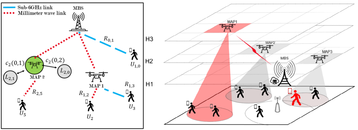
Figure 1: Cell architecture and 3D cell configuration

II-B Channel Model

The channel model varies according to several factors such as the radio environment (i.e. suburban, urban, dense urban, high rise building), the communication band (i.e. sub-6GHz and mm-wave), and the type of communication (i.e. ground-to-ground or ground-to-air). In general, the channel path loss ${\rm PL}_{T}$ for any communication link can be defined on the basis of the Line of Sight (LoS) conditions as follows:

$${\rm PL}_{T}=p{\rm PL}_{Los}+(1-p){\rm PL}_{NLos},$$ (7)

where $p$ is the LoS probability, ${\rm PL}_{Los}$, and ${\rm PL}_{NLos}$ are the LoS and NLoS path loss respectively.
Air/ground sub-6GHz path-loss. Following [15], we define the LoS probability as a function of the elevation angle $\theta$ :

$$p(\theta)=c(\theta-\theta_{0})^{d},$$ (8)

where $\theta_{0}=15^{\circ}$ is the lowest possible angle and $c,d$ are environmental parameters, and we compute the frequency-dependent path loss model as a function of the link type $l\in\{\rm Los,NLos\}$:

$${\rm PL}_{l}=20\mathrm{log}_{10}(d)+20\mathrm{log}_{10}(f)-27.55+\chi_{\sigma_{l}}.$$ (9)

Here, $d$ the distance between the transmitter and the receiver, $f$ is the carrier frequency in $\mathrm{MHz}$, and $\chi_{\sigma_{l}}$ is the shadowing coefficient, which follows a normal distribution with a mean $\mu_{l}$ and a standard deviation $\sigma_{l}$, whose values are given in [15].
Air/ground mm-wave path-loss. Here, we define the LoS probability as a function of the height of the transmitter ($h_{t}$) and receiver ($h_{r}$) and some environmental parameters [16]:

$$p(d)=\prod_{n=0}^{\mathclap{\max(0,\gamma(d))}}1-e^{\left(-\frac{\gamma(d)\max(h_{t},h_{r})-(n+\frac{1}{2})(\left|h_{t}-h_{r}\right|)^{2}}{2\epsilon^{2}\gamma(d)^{2}}\right)}.$$ (10)

In (10), $\gamma(d)$ represents the average number of buildings crossing the link between the transmitter and the receiver separated by a distance $d$. Hence, the distance-dependent path loss model is [17]:

$${\rm PL}_{l}=\alpha_{l}+10\beta_{l}\mathrm{log}_{10}(d)+\chi_{\sigma_{l}};~{}l\in\{\rm Los,NLos\},$$ (11)

where, $\alpha_{l}$, $\beta_{l}$ depend on the radio environment.
Ground/ground sub-6GHz or mm-wave path-loss. Here, the path loss model can be defined without considering the LoS probability [18]:

$${\rm PL}_{T}(d)=10\alpha\mathrm{log}_{10}(d)+\beta+10\gamma\mathrm{log}_{10}(f)+\chi_{\sigma}.$$ (12)

Where $d$ is the distance between the transmitter and the receiver, $f$ the carrier frequency and $\chi_{\sigma}$ the shadowing effect.

II-C Formulation of MAP Deployment Problem

After the above definitions, we formulate the MAP deployment problem to minimize the total deployment cost as:

$$\operatorname*{minimize}_{x_{i,j},\ell_{i,k}}~{} \frac{1}{T}\sum_{t=0}^{T-1}C(t) \mathcal{P}_{1}$$ ()

s.t. $$x_{i,j}(t),~{}\ell_{i,k}(t)\in\{0,1\}, \forall i,j,k,t \mathcal{C}_{1}$$ ()

$$C_{i}(t)\leq C_{\max}, \forall i\in\mathcal{A}\backslash\{0\} \mathcal{C}_{2}$$ ()

$$\sum_{j\in\mathcal{U}}x_{i,j}(t)\leq N_{i}, \forall i,t, \mathcal{C}_{3}$$ ()

$$\sum_{i\in\mathcal{A}}x_{i,j}(t)=1,~{}~{} \forall j,t, \mathcal{C}_{4}$$ ()

$$\kappa_{j}(t)\geq\mathcal{Q}_{j}, \forall j,t, \mathcal{C}_{5}$$ ()

$$\sum_{\mathclap{k\in\mathcal{L}_{i}(t)}}\ell_{i,k}(t)\leq 1, \forall t,i\in\mathcal{A}\backslash\{0\}, \mathcal{C}_{6}$$ ()

$$\sum_{\mathclap{i\in\mathcal{A}\backslash\{0\}}}\quad\sum_{~{}~{}\mathclap{k\in\mathcal{L}_{i}(t)}}\ell_{i,k}(t)\leq K_{\max}, \forall t, \mathcal{C}_{7}$$ ()

The constraint ($\mathcal{C}_{1}$) defines $x_{i,j}$ and $\ell_{i,k}$ as binary variables. The constraint ($\mathcal{C}_{2}$) ensures that the deployment cost of a MAP is lower than the maximum cost $C_{\max}$. The constraints ($\mathcal{C}_{3}$) and ($\mathcal{C}_{4}$) ensure that each AP $i$ serves at most $N_{i}$ UEs and that each UE is associated to exactly one AP. The constraint ($\mathcal{C}_{5}$) guarantees the QoS satisfaction of each UE. Finally, the constraints ($\mathcal{C}_{6}$)-($\mathcal{C}_{7}$) guarantees that a MAP is deployed to at most one location at a time and that the total number of deployed MAP does not exceed $K_{\max}$. It is worth noting that Problem ($\mathcal{P}_{1}$) is non-convex and NP-hard, thus difficult to solve with classical optimizations techniques.

III Proposed Solution

Our proposed solution for deploying MAPs jointly considers the deployment cost, UEs’ mobility, co-channel interference, and traffic request dynamic. One key challenge is that the optimal MAP deployment strategy strongly depends on UEs’ traffic requests and the co-channel interference that will be generated, which is not known until UEs are fully associated. At the same time, the optimal association of UEs also depends on the MAP deployment. This ping-pong effect makes the problem very complex and difficult to solve. To limit such a complexity, we first define a 3D grid of positions for MAPs. The discretization of the 3D space gives a finite number of solutions for the problem $\mathcal{P}_{1}$. However, the search space of possible solutions remains large, prohibiting any exhaustive search approach. Thus, we design SIMBA, a Scalable Iterative Monte-Carlo Based Algorithm, with low-complexity, which explores the search space to find (sub)-optimal solutions as illustrated in in Fig. 2. SIMBA, first performs Monte-Carlo explorations of MAPs deployment strategies and then exploits the best solution by adopting a standard user association algorithm based on maximum Signal-to-noise-ratio (MAX-SNR) to find the sub-optimal MAP deployment with low complexity. Next, based on SIMBA output, we apply our previously proposed MARL framework to train a user association, which in contrast to the MAX-SNR algorithm, considers co-channel interference. We show that this approach is able to compensate the sub-optimality of SIMBA.

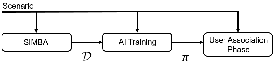
Figure 2: Proposed solution architecture

III-A SIMBA: Scalable Iterative Monte-Carlo Based Algorithm

This section describes SIMBA, a low-complexity iterative algorithm (see Algorithm 1), which finds near-optimal MAPs deployment solution (in terms of deployment cost and UEs’ QoS satisfaction). SIMBA alternates a Monte-Carlo exploration and exploitation phases. During an exploration, SIMBA randomly samples a set $\mathcal{M}_{k}$ of $k$ locations on which MAPs are deployed. Each time it deploys a MAP $i$ on a location $p$, it updates a score associated to this location. Let $\mathrm{score}_{p}^{(i)}(t)$ be such a score:

$$\mathrm{score}_{p}^{(i)}(t)=\frac{1}{|\mathcal{U}_{i}|}\sum_{j\in\mathcal{U}_{i}}\kappa_{j}(t),$$ (13)

where $\mathcal{U}_{i}$ is the number of UEs served by MAP $i$. As we consider interference and mobility, the score of a position is computed based on UEs’ perceived QoS. Thus, higher the score, better the QoS of UEs served by a MAP deployed at that position. In the exploitation phase, a MAP is deployed at the location with the highest score. This location is no longer sampled until a solution of $\mathcal{P}_{1}$ has been found. Then we iterate over $T$ episodes at the end of which we select the best solution of MAPs deployment $\mathcal{D}$. Eventually, given $\mathcal{D}$, we learn the optimal user association using a multi-agent reinforcement learning based approach.

Input: Define the set of MAPs possible locations $\mathcal{L}$ and the number of Monte-Carlo iterations $M$.

Initialize the score of locations: $\mathrm{score}_{p}=0,~{}\forall p\in\mathcal{L}$.

Initialize the set of deployed MAP locations $\mathcal{D}=\emptyset$.

Set $C_{\min}=\infty$ and $k=K_{\max}$ (max. number of UAVs)

for $t=1,\dots,T$ do

       Initialize an empty set of locations $\mathcal{D}_{t}=\emptyset$.

       for $s=1\dots K_{\max}$ do

             Step 1: Monte-Carlo exploration

             for $m=1,\dots,M$ do

                   Randomly sample $k$ locations $\mathcal{M}_{k}(m)\sim\mathcal{L}$.

                   Deploy a UAV to location $p,~{}\forall p\in\mathcal{M}_{k}(m)$.

                   Perform user association procedure¹.

                   for $p\in\mathcal{M}_{k}(m)$ do

                         Compute the score of $p$ using Eq. (13).

                         Update $\mathrm{score}_{p}$ of location $p$.

                   end for

                  

             end for

            Step 2: Monte-Carlo exploitation

             Store location $i=\operatornamewithlimits{arg\,max}_{i}\{\mathrm{score}_{i}\}$ in $\mathcal{D}_{t}$.

             Deploy UAVs into the locations in $\mathcal{D}_{t}$.

             Compute $C(t)$, and $\kappa_{j}(t),~{}\forall j$.

             if ($\mathcal{C}_{1}$)-($\mathcal{C}_{7}$) are guaranteed then

                   Break.

                  

            else

                   Remove $i$ from $\mathcal{L}$ and set $k=k-1$.

                  

             end if

            

       end for

      Step 3: Test Monte-Carlo solution

       if $C(t)<C_{\min}$ then

             $C_{\min}=C(t)$

             Save current deployment $\mathcal{D}=\mathcal{D}_{t}$

       end if

      

end for

Output: $\mathcal{D}$ set of locations of deployed MAPs

¹Note: Here, we adopt the MAX-SNR algorithm to limit complexity.

Algorithm 1 SIMBA MAP Deployment Algorithm

III-B User Association

In this section, we describe the proposed MARL algorithm for user association. In the proposed framework, we model each UE as an agent, which cooperatively learns with its teammates a common user association policy through interaction with the shared radio environment. To this end, agents learn to map their local and global observations $o_{j}(t)$ of the radio environment to actions $a_{j}(t)$ corresponding to connection requests towards MAPs. Following our previous work [19], let $o_{j}^{l}(t)=\{R_{\alpha}(t),{\rm RSS}_{j}(t),{\rm AoA}_{j}(t),R_{a_{j}(t),j}(t),D_{j}(t)\}$ denote the local observation, which comprises the received signal strength $\mathrm{RSS}_{j}$, and the associated angle of arrival $\mathrm{AoA}$ w.r.t to all MAPs. Here, $R_{a_{j}(t),j}(t)$ represents UE $j$’s perceived rate and $D_{j}(t)$ the UE $j$ data demand. Moreover let $o_{j}^{g}(t)=\{(x_{k}(t),y_{k}(t),z_{k}(t),a_{k}(t-1)),~{}\forall k\in\mathcal{N}_{j}(t)\}$ denote the global observations of UE $j$, where $(x_{k}(t),y_{k}(t),z_{k}(t))$ is the location of its $k$-th neighbors, $a_{k}(t-1)$ is the connection request in previous time slot, and $\mathcal{N}_{j}(t)$ denotes the UE neighborhood. This global observations represent UE $j$ perception of its surrounding environment. The goal of the learning procedure is to define the user association policy $\pi_{\boldsymbol{\mathrm{w}}}$, with learnable weights $\boldsymbol{\mathrm{w}}$, which outputs the association probability vector $p_{j}(t)=\pi(o_{j}(t))\in\mathbb{R}^{|\mathcal{A}|}$ that maximizes the sum of $\gamma$-discounted rewards over a time horizon $T_{e}$:

$$G_{j}(t)=\sum_{\tau=t+1}^{T_{e}}\gamma^{\tau-t-1}R_{\alpha}(\tau),$$ (14)

where $\gamma$ is the discount factor such that $0<\gamma<1$. Finally, we construct the policy $\pi_{\boldsymbol{\mathrm{w}}}$ using an actor-critic module, which is optimized via proximal policy optimization [19]. In particular, our proposed solution is specifically conceived to handle dynamic networks with varying number and position of UEs.

III-C Complexity Analysis

As we discretize the 3D-space, a naive algorithm may find the optimal solution of problem $\mathcal{P}_{1}$ using an exhaustive search. This algorithm has a complexity of $\mathcal{O}(C)$, where $C=\sum_{i=0}^{K_{\max}}\begin{pmatrix}|\mathcal{L}|\\ i\end{pmatrix}$ is the number of possible combinations of locations. In the worse case scenario where $K_{\max}\geq\frac{|\mathcal{L}|}{2}$, we have $C\geq 2^{|\mathcal{L}|-1}$. Note that each combination is not guaranteed to solve $\mathcal{P}_{1}$, which also requires solving the user association, leading to a prohibitive solution with very high complexity. In contrast, SIMBA has a complexity of approximately $\mathcal{O}(TMK_{\max})$, which scales linearly with $T$ and the number of Monte-Carlo iterations $M$ that we can conveniently choose to find (sub)-optimal solutions in a reasonable time.

IV Numerical Results

Here, we assess the performance of our proposed MAP deployment method on dynamic scenarios at different scales. The first scenario, named SmallScale, is a small scale deployment of $10$ UEs randomly and $4$ MAPs moving through 12 positions at 3 different altitudes (i.e. $15$, $35$ and $50~{}\mathrm{m}$) in a $100~{}\mathrm{m}$ by $100~{}\mathrm{m}$ area. In this scenario, we can easily compare our method with brute force mechanism, named Exhaustive, without too high computational time. The MediumScale scenario is made with $40$ UEs and $10$ MAPs moving through $27$ positions at $3$ altitudes in a $200~{}\mathrm{m}$ by $200~{}\mathrm{m}$ area. The UEs are deployed with uniform probability and move randomly over the cell. The UEs’ traffic follows a Poisson distribution bit/s and simulates dynamic rate demand. Both scenarios include a baseline random algorithm, named Random, where the deployment decision and the chosen location follow a uniform law $U(0,1)$. Thus each UAV chooses a random location and when a better combination is found, the solution is updated.

Concerning MAPs, each UAV has a coverage range defined by the aperture angle of its antenna to ground UEs and its altitude. At most $K=10$ UAVs can de deployed and each UAV can connect to at most $N_{i}=10$ UEs. We fix the rent cost $c_{i,0}=c_{0}=1,~{}\forall i$, so that we can omit it from the optimization in Eq. (1). Table I gives an overview of the simulation parameters.

TABLE I: Simulation Parameters

Scenario Parameters	Small Scale	Medium Scale
Cell size	$100\times 100~{}\mathrm{m}$	$200\times 200~{}\mathrm{m}$
Number of UEs	$10$	$40$
Number of positions	$4\times 3=12$	$9\times 3=27$
UE Mobility	Random Walk
Avg. traffic demand $D_{j}(t)$	$200~{}\mathrm{Mbps}$
Channel Parameters	MBS	BS/UAV
Carrier Frequency $f_{c}$	$2~{}\mathrm{GHz}$	$28~{}\mathrm{GHz}$
Bandwidth	$10~{}\mathrm{MHz}$	$500~{}\mathrm{MHz}$
Thermal Noise $N_{0}$	$-174~{}\mathrm{dBm}/~{}\mathrm{Hz}$
Shadowing power $\sigma^{2}$	$9~{}\mathrm{dB}$	$12~{}\mathrm{dB}$
Transmit Power	$46~{}\mathrm{dBm}$	$20~{}\mathrm{dBm}$
Antenna Gain	17 dBi	Directive [19]
UAV Aperture	$120\deg$
Altitude	$[10,35,50]~{}\mathrm{m}$

IV-A Drone Deployment

We set $M=10$ and $T=100$ in SIMBA and average the results over $30$ Monte-Carlo simulations. We conveniently fix the QoS’s target of ($\mathcal{C}_{5}$) to $Q_{j}=100\%$ for SmallScale and $Q_{j}=85\%$ for MediumScale due to limited radio resources. We first assess the deployment cost of our proposed solution compared to the two benchmarks as shown in Fig. 3. Our algorithm converges faster than a naive random approach to a close optimal-solution. In a high mobility context, it is important to obtain a flexible algorithm that finds a solution faster than the network changes.

Moreover, our algorithm guarantees not to deploy more drones than needed, which may imply a high cost. Meanwhile, as shown in Fig. 4.a, our solution ensures and guarantees the targeted QoS for UEs in both small and medium scale scenarios with less MAPs compared to a naive approach as illustrate 4.b. Finally, as we added more potential locations for UAVs in MediumScale scenario, our solution is better at identifying the best combinations than a random naive approach and faster than an exhaustive solution, thus, guaranteeing a near-optimal solution with $4.22$ UAVs deployed in average.

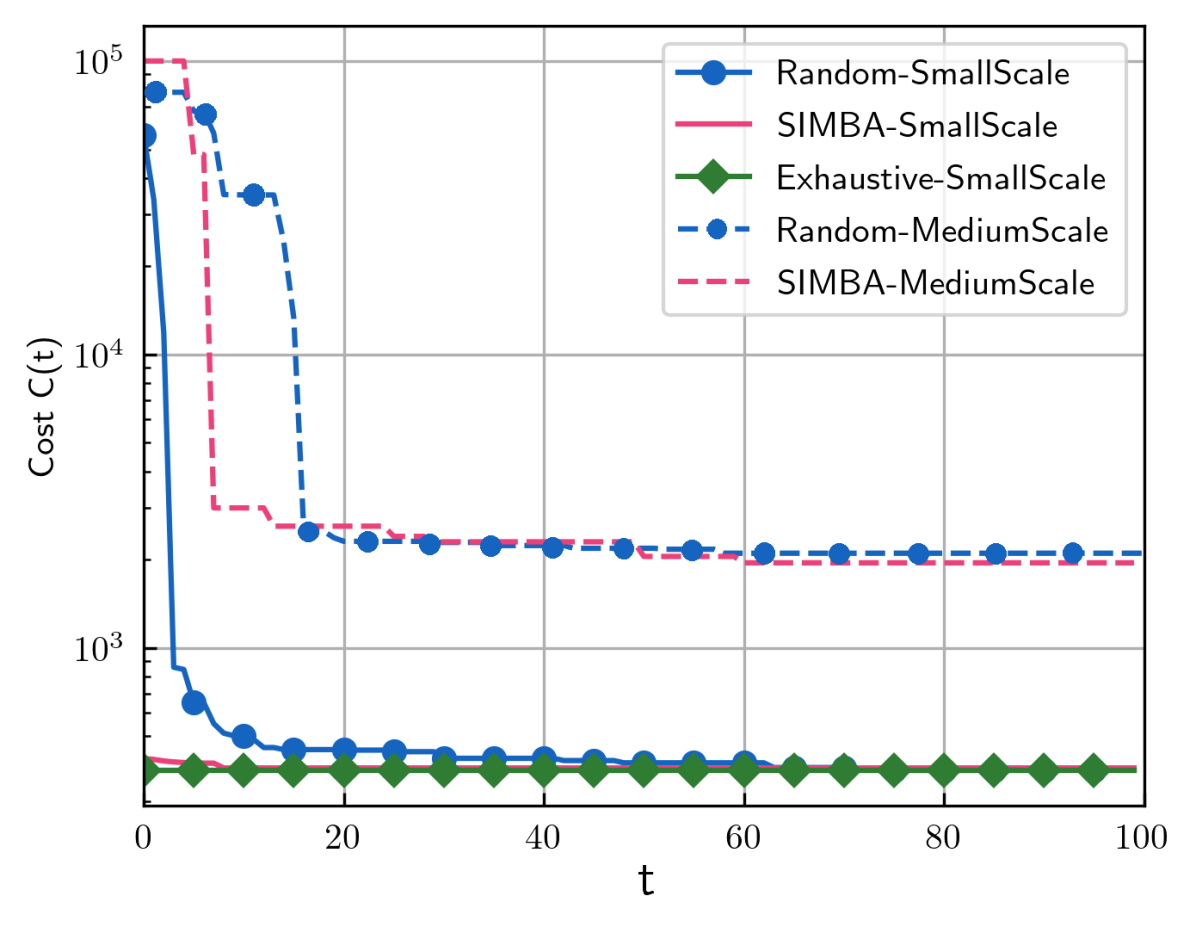
Figure 3: MAP deployment cost for each method and for both scenarios as a function of the number of iterations.

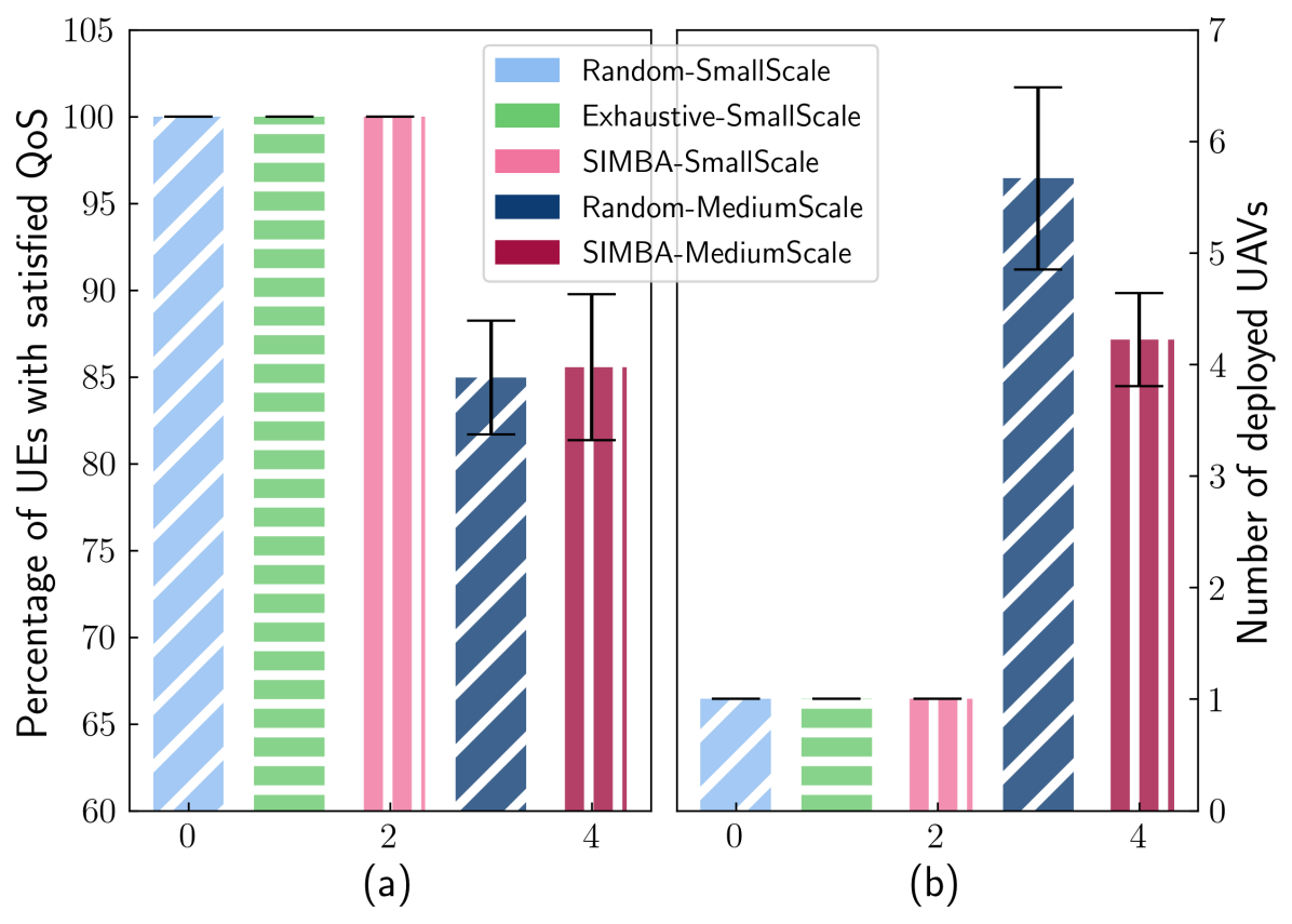
Figure 4: (a) Average percentage of UEs with satisfied QoS and (b) average number of UAVs deployed for both scenarios and for each method.

IV-B User Association

To train the user association policy, we use the MARL framework described in section III-B. All simulation results are plotted for a learning rate $\mu=10^{-4}$ and a discount factor $\gamma=0.6$. The MARL agents are trained for $T_{e}=3000$ episodes. Agents are trained with $\alpha=1$ for the $\alpha$-fair utility function, meaning that the agents are trained on a fair sum-rate setting. Note that all the hyperparameters were determined empirically. We perform several deployments and trainings with increasing number of MAPs and compare the proposed solution to the MAX-SNR-based approach for MediumScale scenario. Here, results are averaged over $300$ simulations with $T=150$ iterations. Fig. 5 shows the impact of increasing the number of UAVs on the network performance. We observe that, for a number of deployed UAVs greater than tree, our proposed approach increases the log network sum-rate by $1.5\%$, implying a network sum-rate enhancement by nearly $30\%$ compared to MAX-SNR algorithm. Moreover, for the given scenario, Fig. 5 illustrates the trade-off between drone deployment and UE QoS. With more than $4$ UAVs deployed, the log sum-rate barely varies. This result confirms that when interference is taken into account, increasing the number of access points does not necessarily implies better UE’s QoS at the risk of increasing the deployment cost.

Next, in the MediumScale scenario, we increase the user density $\lambda(\mathrm{UEs}/\mathrm{m}^{2})$ to show the effectiveness of our solution in this complex setting. Fig. 6 compares the average handover frequency and the network log sum-rate as a function of user density $\lambda$. The increase of $\lambda$ ultimately increases the number of handovers frequency for the MAX-SNR algorithm as multiple UEs compete for the same resources. In contrast, our proposed solution guarantees stable performance due to its capability to to balance the network load, especially in dense deployment scenarios. As shown in Fig. 6, our proposed solution improves the log network sum-rate by $4\%$, which implies an increase in network sum-rate by $60\%$ compared to a MAX-SNR algorithm, in particular for dense deployment scenario (e.g. $\lambda=9\times 10^{-3}\mathrm{UEs}/~{}\mathrm{m}^{2}$).

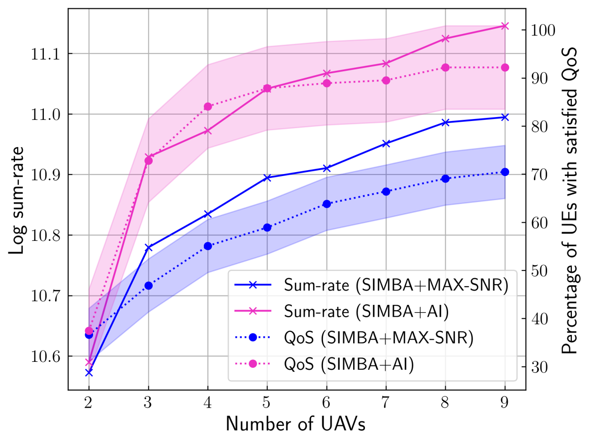
Figure 5: Average network log sum-rate and average percentage of UEs with QoS satisfaction as a function of the number of deployed UAVs for MediumScale scenario for both UE association algorithms.

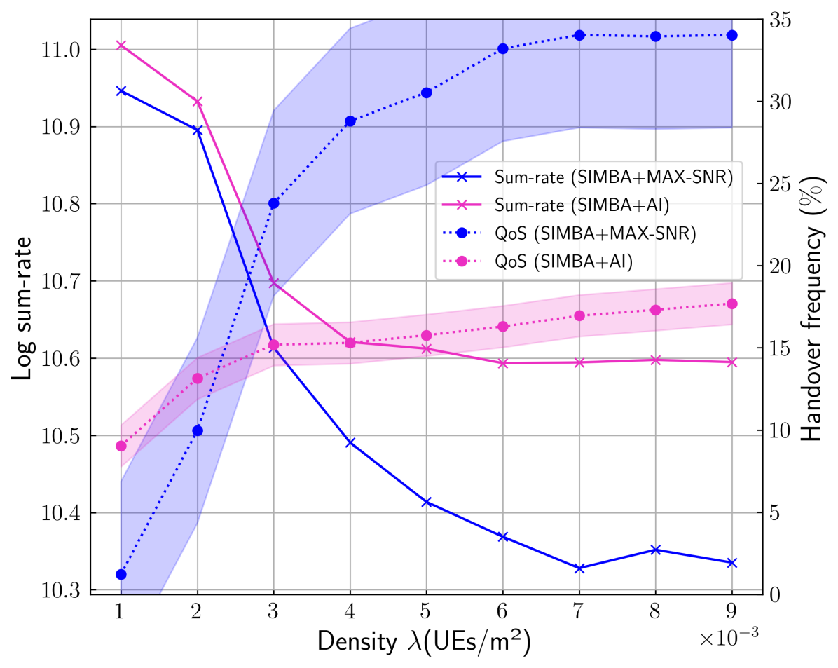
Figure 6: Average network log sum-rate and average handover frequency as a function of the user density.

V Conclusion

In this paper, we proposed an algorithm to solve the joint problem of MAP deployment and user association while taking into account UE mobility, UE demand and network interference. The algorithm finds the MAP positions in a 3D space and optimizes the user association for a given network configuration. The proposed algorithm is the first step for more complex scenarios. We will consider path planning optimization to exploit MAP connectivity while moving within the network, include the backhaul constraint and optimization and extend our study to more realistic configurations with aerial and ground base stations.

References

- [1] Y. Zeng, Q. Wu, and R. Zhang, “Accessing From the Sky: A Tutorial on UAV Communications for 5G and Beyond,” Proceedings of the IEEE, vol. 107, no. 12, pp. 2327–2375, 2019.
- [2] N. H. Z. Lim, Lee, et al., “Coverage Optimization for UAV Base Stations using Simulated Annealing,” in 2021 IEEE Malaysia International Conference on Communication (MICC), pp. 43–48, 2021.
- [3] M. Peer, V. A. Bohara, and A. Srivastava, “Multi-UAV Placement Strategy for Disaster-Resilient Communication Network,” in Proc. IEEE Vehicular Technology Conference (VTC2020-Fall), pp. 1–7, 2020.
- [4] S. Sharafeddine and R. Islambouli, “On-Demand Deployment of Multiple Aerial Base Stations for Traffic Offloading and Network Recovery,” CoRR, vol. abs/1807.02009, 2018.
- [5] J. Sabzehali, V. K. Shah, Q. Fan, B. Choudhury, L. Liu, and J. H. Reed, “Optimizing Number, Placement, and Backhaul Connectivity of Multi-UAV Networks,” CoRR, vol. abs/2111.05457, 2021.
- [6] R. Ghanavi, E. Kalantari, et al., “Efficient 3d aerial base station placement considering users mobility by reinforcement learning,” CoRR, vol. abs/1801.07472, 2018.
- [7] Y. Li et al., “UAV-Assisted Cellular Communication: Joint Trajectory and Coverage Optimization,” in Proc. IEEE Wireless Communications and Networking Conference (WCNC), pp. 1–6, 2021.
- [8] Q. Zhang, Saad, et al., “Predictive Deployment of UAV Base Stations in Wireless Networks: Machine Learning Meets Contract Theory,” IEEE Trans. on Wireless Communications, vol. 20, no. 1, pp. 637–652, 2021.
- [9] Z. Li, Y. Wang, et al., “Efficient Resource Allocation in UAV-BS Dual Connectivity Heterogeneous Networks,” in Proc. International Conference on Information Science and Technology, pp. 234–239, 2019.
- [10] X. Sun, N. Ansari, and R. Fierro, “Jointly Optimized 3D Drone Mounted Base Station Deployment and User Association in Drone Assisted Mobile Access Networks,” IEEE Transactions on Vehicular Technology, vol. 69, no. 2, pp. 2195–2203, 2020.
- [11] E. Kalantari, I. Bor-Yaliniz, et al., “User association and bandwidth allocation for terrestrial and aerial base stations with backhaul considerations,” CoRR, vol. abs/1709.07356, 2017.
- [12] M. Sana, A. De Domenico, W. Yu, Y. Lostanlen, and E. Calvanese Strinati, “Multi-Agent Reinforcement Learning for Adaptive User Association in Dynamic mmWave Networks,” IEEE Transactions on Wireless Communications, vol. 19, no. 10, pp. 6520–6534, 2020.
- [13] H. V. Abeywickrama et al., “Comprehensive Energy Consumption Model for Unmanned Aerial Vehicles, Based on Empirical Studies of Battery Performance,” IEEE Access, vol. 6, pp. 58383–58394, 2018.
- [14] E. Altman, K. Avrachenkov, and A. Garnaev, “Generalized -fair resource allocation in wireless networks,” in Proc. IEEE Conference on Decision and Control, pp. 2414–2419, 2008.
- [15] A. Al-Hourani, S. Kandeepan, and A. Jamalipour, “Modeling air-to-ground path loss for low altitude platforms in urban environments,” in Proc. IEEE Global Communications Conference, pp. 2898–2904, 2014.
- [16] W. Yi, Y. Liu, E. Bodanese, A. Nallanathan, and G. K. Karagiannidis, “A Unified Spatial Framework for UAV-Aided MmWave Networks,” IEEE Transactions on Communications, vol. 67, no. 12, pp. 8801–8817, 2019.
- [17] H. Shakhatreh, W. Malkawi, A. Sawalmeh, M. Almutiry, and A. Alenezi, “Modeling Ground-to-Air Path Loss for Millimeter Wave UAV Networks,” CoRR, vol. abs/2101.12024, 2021.
- [18] S. Sun, T. S. Rappaport, et al., “Propagation Path Loss Models for 5G Urban Micro- and Macro-Cellular Scenarios,” in Proc. IEEE Vehicular Technology Conference (VTC Spring), pp. 1–6, 2016.
- [19] M. Sana, N. di Pietro, and E. Calvanese Strinati, “Transferable and Distributed User Association Policies for 5G and Beyond Networks,” in Proc. IEEE International Symposium on Personal, Indoor and Mobile Radio Communications (PIMRC), pp. 966–971, 2021.