Restarted randomized surrounding methods for solving large linear equations

Abstract

A class of restarted randomized surrounding methods are presented to accelerate the surrounding algorithms by restarted techniques for solving the linear equations. Theoretical analysis shows that the proposed method converges under the randomized row selection rule and the convergence rate in expectation is also addressed. Numerical experiments further demonstrate that the proposed algorithms are efficient and outperform the existing method for overdetermined and underdetermined linear equations, as well as in the application of image processing.

Keywords. Reflection transformation, Randomized iterative methods, Linear equations, Convergence

1 Introduction

Consider the solution of linear algebraic equations

$$Ax=b,\quad A\in\mathbb{R}^{m\times n},\quad b\in\mathbb{R}^{m},$$ (1.1)

where $A$ has full column rank, which comes widely from many scientific and engineering computation, for instance, discrete PDEs, image reconstruction, signal processing, option pricing and machine learning.

Kaczmarz method is one of the well-known iterative projection method, which was firstly proposed in [11] and further extended to block and inconsistent cases in [9, 6]. Since the linear convergence of a randomized Kaczmarz method was established by Strohmer and Vershynin [14], variants of randomized Kaczmarz method were presented and deeply studied, see [3, 4, 10, 8]. On the other hand, iterative methods based on Householder orthogonal reflection also attract much attention from the community of numerical linear algebra. Cimmino [7] firstly proposed a general iteration scheme with orthogonal reflection and proved the convergence as long as the rank of $A$ is greater than one. Ansorge [1] gave the relations between the Cimmino method and Kaczmarz method for the solution of singular and rectangular systems of equations and proved the rate of convergence for a given weight. Further, block Cimmino method[2, 15] and extended Cimmino method [12] were proposed and investigated. For more details of the Cimmino method, we refer the reader to [5].

Recently, Steinerberger[13] studied a surrounding method which randomly reflected the start point and took the average of all reflective points as the approximate solution. In this manuscript, we propose a restarted randomized surrounding method, which takes the average of several randomly reflective points as the new initial value and repeats the iterations. Theoretical analysis demonstrates the convergence in expectation and shows the convergence rate is faster than that of the existing surrounding method. Numerical experiments further verify our analysis, and show that restarted strategies are efficient which can greatly accelerate the surrounding method.

The organization of the rest paper is as follows. In Section 2, we give some notations and propose the restarted randomized surrounding algorithms. In Section 3, the convergence analysis is given and compared with the existing results. Numerical experiments are presented in Section 4 compared with the surrounding method. Finally, in Section 5, we end this paper with the conclusions.

2 The restarted randomized surrounding method

In this section, after introducing the notations and reviewing the existing method, we introduce the restarted randomized surrounding method for solving the linear equations (1.1).

Denote $a_{i}^{T}=[a_{i1},a_{i2},\ldots,a_{in}]$ and $b_{i}$ be the $i$th row of $A$ and the $i$th entry of the right-hand side vector $b$ respectively. Let $x_{k}$ be the $k$th approximate solution and $x_{\ast}$ be the exact solution of the linear equations (1.1) respectively, which is actually the intersection of the $n$ hyperplanes $a_{i}^{T}x=b_{i}(1\leq i\leq m)$.

By choosing $i_{k}$ from the set $\left\{1,2,\cdots,m\right\}$ with probability proportional to $\|a_{i}\|_{2}^{2}$, Steinerberger [13] proposed a surrounding method as follows.

$$x_{k+1} = x_{k}+2\frac{b_{i_{k}}-a_{i_{k}}^{T}x_{k}}{\|a_{i_{k}}\|_{2}^{2}}a_{i_{k}},\quad 1\leq k\leq M,$$ (2.1)

$$= (I-2\frac{a_{i_{k}}^{T}a_{i_{k}}}{\|a_{i_{k}}\|_{2}^{2}})x_{k}+2\frac{b_{i_{k}}}{\|a_{i_{k}}\|_{2}^{2}}a_{i_{k}},\quad 1\leq k\leq M.$$ (2.2)

After $M$ reflections, the approximate solution is given by the average of all the reflective points $\frac{1}{M}\sum_{k=1}^{M}x_{k}$.

Steinerberger [13] proved that the approximate solution approaches to the true solution $x_{\ast}$ when $M$ goes to infinity, e.g., $\lim\limits_{M\rightarrow\infty}\frac{1}{M}\sum_{i=1}^{M}x_{k}=x_{\ast}$ and the convergence rate in expectation was given by

$$\mathbb{E}\left\|x_{\ast}-\frac{1}{M}\sum_{k=1}^{M}x_{k}\right\|\leq\frac{1+\|A\|_{F}\left\|A^{-1}\right\|}{\sqrt{M}}\left\|x_{\ast}-x_{0}\right\|.$$ (2.3)

It is easily seen that it requires quite a number of reflective points to achieve a satisfying convergence precision, which is usually very expensive.

In order to accelerate the convergence of the randomized surrounding method, a restarted version is proposed which firstly reflects several times and then takes the average of the reflective points as the initial to restart the iterations.

The framework of the restarted randomized surrounding method (abbreviated as RRS) can be described as follow:

Algorithm 1 Restarted randomized surrounding (RRS) algorithms

1:$A$, $b$, initial guess $x_{0}=y_{0}^{(0)}\in\mathbb{R}^{n}$, restarted number $q$.

2:approximate solution $x_{k+1}$.

3:for $k=0,1,2,\ldots$  do

4:     for  $i=1,2,\ldots,q-1$ do

5:         Select a row index $i_{k}$ randomly according to $p_{i_{k}}=\frac{\|a_{i_{k}}\|^{2}}{\|A\|_{F}^{2}}$

6:         Set $y_{k}^{(i)}=y_{k}^{(i-1)}+2\frac{b_{i_{k}}-a^{T}_{i_{k}}y_{k}^{(i-1)}}{\|a_{i_{k}}\|_{2}^{2}}a_{i_{k}}$

7:     end for

8:     Compute the approximate solution: $x_{k+1}=\frac{1}{q}\sum_{i=0}^{q-1}y_{k}^{(i)}$

9:     Update $y_{k+1}^{(0)}=x_{k+1}$

10:end for

11:return $x_{k+1}$

We plot a sketch graph to demonstrate the idea of restarted randomized surrounding method in Figure 1, where the green diamond points are the approximate solutions which eventually converge to the center, namely the true solution. In Figure 1, the star points and circle points denote the randomized reflective points generated in the first and second loops respectively.

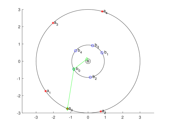
Figure 1: Sketch of restarted randomized surrounding method

3 Convergence analysis

Denote the Householder reflection matrix corresponding to the $i$th hyperplane by

$$H_{i}=I-2\frac{a_{i}a_{i}^{T}}{a_{i}^{T}a_{i}},\quad i=1,2,\ldots,m.$$ (3.1)

which is an $n\times n$ orthogonal matrix. We give the convergence of restarted randomized surrounding method as follows.

Lemma 3.1.

In every iteration, if $q$ reflections are randomly computed where $i_{k}$ is taken from the set $\left\{1,2,\cdots,m\right\}$ with the probability $p_{i_{k}}=\frac{\|a_{i_{k}}\|^{2}}{\|A\|_{F}^{2}}$, then the sequence $\{\|x_{k}-x_{\ast}\|\}$ is non-increasing.

Proof.

Without loss of generality, we assume that the rows with indices $\{i_{1},\ldots,i_{q}\}$ are selected in $k$-th iteration step and set

$$Q_{j}=H_{i_{j}}H_{i_{j-1}}\cdots H_{i_{1}},\,Q_{0}=I,\,j=1,\ldots,q.$$ (3.2)

where $I$ represents the identity matrix of size $n$. Since $Q_{j}$ is a product of the Householder matrices, $Q_{j}$ is orthogonal and nonsingular. Hence,

$$x_{k+1}-x_{\ast} =\frac{1}{q}\left(\sum_{i=1}^{q}y_{k}^{(i)}\right)-x_{\ast}$$ (3.3)

$$=\frac{1}{q}\sum_{i=1}^{q}(y_{k}^{(i)}-x_{\ast})$$

$$=\frac{1}{q}(Q_{1}+Q_{2}+\cdots+Q_{q})(x_{k}-x_{\ast}).$$

Due to distance-preserving transformation,

$$\|x_{k+1}-x_{\ast}\|\leq\frac{1}{q}\sum_{j=1}^{q}\|Q_{j}(x_{k}-x_{\ast})\|=\frac{1}{q}\sum_{i=1}^{q}\|(x_{k}-x_{\ast})\|=\|(x_{k}-x_{\ast})\|.$$ (3.4)

Because the linear combination is convex, the equality in (3.4) holds if and only if

$$x_{k}-x_{\ast}=Q_{1}(x_{k}-x_{\ast})=\cdots=Q_{q}(x_{k}-x_{\ast}).$$

If $x_{k}\not=x_{\ast}$ and $\mathcal{N}(A)=\{0\}$, then $\|\frac{1}{q}(Q_{1}+Q_{2}+\cdots+Q_{q})\|<1$, which yields the sequence $\{\|x_{k}-x_{\ast}\|\}$ is decreasing.  

From the Lemma 3.1, it is seen that the restarted randomized surrounding algorithm is convergent. Further, we estimate and analyze the convergence rate of the restarted randomized surrounding algorithm as follow.

Theorem 3.1.

If $i_{k}$ is taken with the probability $p_{i_{k}}=\frac{\|a_{i_{k}}\|^{2}}{\|A\|_{F}^{2}}$ and $q$ reflections are randomly taken in every iteration, it holds

$$\mathbb{E}\|x_{\ast}-x_{k}\|^{2}\leq\gamma^{k}\|x_{0}-x_{\ast}\|^{2},\quad 0<\gamma<1,$$ (3.5)

where the constant $\gamma<\frac{1}{q}+\frac{2}{q^{2}}\sum_{i=1}^{q-1}(q-i)\|\mathcal{L}\|^{i}$ and $\|\mathcal{L}\|=1-\frac{2\sigma_{\min}^{2}}{\|A\|_{F}^{2}}$.

Proof.

Denote $\langle\cdot,\cdot\rangle$ be the Euclidean inner product, for all $x,y\in\mathbb{R}^{n}$, $i_{j}\in\{1,2,\ldots,m\}$, we have

$$\mathbb{E}_{i_{j}}\left(\langle y,Q_{j}x\rangle\right)=\mathbb{E}_{i_{j}}\left(\langle y,(I-2\frac{a_{i_{j}}a_{i_{j}}^{T}}{\|a_{i_{j}}\|^{2}})Q_{j-1}x\rangle\right)$$ (3.6)

$$= \langle y,Q_{j-1}x\rangle-2\mathbb{E}_{i_{j}}\left(\langle y,\frac{a_{i_{j}}a_{i_{j}}^{T}}{\|a_{i_{j}}\|^{2}}Q_{j-1}x\rangle\right)$$

$$= \langle y,Q_{j-1}x\rangle-2\langle y,\sum_{j=1}^{m}\frac{\|a_{i_{j}}\|^{2}}{\|A\|_{F}^{2}}\left(\frac{a_{i_{j}}a_{i_{j}}^{T}}{\|a_{i_{j}}\|^{2}}Q_{j-1}x\right)\rangle$$

$$= \langle y,Q_{j-1}x\rangle-\frac{2}{\|A\|_{F}^{2}}\sum_{j=1}^{m}y^{T}a_{i_{j}}a_{i_{j}}^{T}Q_{j-1}x$$

$$= \langle(I-\frac{2}{\|A\|_{F}^{2}}A^{T}A)y,Q_{j-1}x\rangle:=\langle\mathcal{L}y,Q_{j-1}x\rangle.$$

Similarly, it is obtained that

$$\mathbb{E}_{i_{1},i_{2},\ldots,i_{j}}\langle y,Q_{j}x\rangle=\mathbb{E}_{i_{1},i_{2},\ldots,i_{j-1}}\langle\mathcal{L}y,Q_{j-1}x\rangle=\mathbb{E}_{i_{1},i_{2},\ldots,i_{j-2}}\langle\mathcal{L}^{2}y,Q_{j-2}x\rangle=\cdots=\langle\mathcal{L}^{j}y,x\rangle.$$ (3.7)

Since $\mathcal{L}=I-\frac{2}{\|A\|_{F}^{2}}A^{T}A$ is a symmetric matrix,

$$\rho(\mathcal{L})=\|\mathcal{L}\|\leq 1-\frac{2\sigma_{\min}^{2}}{\|A\|_{F}^{2}},$$ (3.8)

where $\sigma_{\min}$ is the smallest singular value of $A$. Thus,

$$|\mathbb{E}_{i_{1},i_{2},\ldots,i_{j}}\langle x,Q_{j}x\rangle|\leq\|\mathcal{L}^{j}x\|\|x\|\leq\|\mathcal{L}\|^{j}\|x\|^{2}.$$

Let $e_{k}=x_{k}-x_{\ast}$ and it holds that

$$\mathbb{E}\|x_{\ast}-x_{k+1}\|=\mathbb{E}\|x_{\ast}-\frac{1}{q}\sum_{j=0}^{q-1}Q_{j}x_{k}\|^{2}=\frac{1}{q^{2}}\mathbb{E}\|\sum_{j=0}^{q-1}Q_{j}e_{k}\|^{2}$$ (3.9)

$$=\frac{1}{q^{2}}\left[\sum_{j=0}^{q-1}\langle Q_{j}e_{k},Q_{j}e_{k}\rangle+2\mathbb{E}\sum_{j=0}^{q-2}\sum_{\ell=j+1}^{q-1}\langle Q_{j}e_{k},Q_{\ell}e_{k}\rangle\right]$$

$$=\frac{1}{q}\|e_{k}\|^{2}+\frac{2}{q^{2}}\mathbb{E}\sum_{j=0}^{q-2}\sum_{\ell=j+1}^{q-1}\langle Q_{j}e_{k},H_{i_{\ell}}\cdots H_{i_{j+1}}(Q_{j}e_{k})\rangle$$

$$\leq\frac{1}{q}\|e_{k}\|^{2}+\frac{2}{q^{2}}\sum_{j=0}^{q-2}\sum_{\ell=j+1}^{q-1}\|\mathcal{L}^{\ell-j}\|\|Q_{j}e_{k}\|^{2}:=\gamma\|e_{k}\|^{2},$$

where $\gamma$ is a constant and $\|\mathcal{L}\|<1$. By calculating,

$$\gamma =\frac{1}{q}+\frac{2}{q^{2}}\left[(q-1)\|\mathcal{L}\|+(q-2)\|\mathcal{L}^{2}\|+\cdots+\|\mathcal{L}^{q-1}\|\right]$$

$$\leq\frac{1}{q}+\frac{2}{q^{2}}\left[(q-1)\|\mathcal{L}\|+(q-2)\|\mathcal{L}\|^{2}+\cdots+\|\mathcal{L}\|^{q-1}\right]<1.$$

Hence, it holds that

$$\mathbb{E}\|x_{\ast}-x_{k+1}\|^{2}\leq\gamma\|x_{k}-x_{\ast}\|^{2}\Rightarrow\mathbb{E}\|x_{\ast}-x_{k}\|^{2}\leq\gamma^{k}\|x_{0}-x_{\ast}\|^{2}.$$

 

As a consequence of Theorem 3.1, when the restarts are carried out every $q$ reflection for $k$ times, i.e., total $kq$ iterations, then the convergence rate of restarted randomized surrounding method is $\gamma^{k}=O(\frac{1}{q^{k}})$, which is much less that $O(\frac{1}{kq})$, the rate of the randomized surrounding method if $k>2$ and $q>2$. It shows the potential that the restarted version could be faster than the original one.

The restarted randomized surrounding method can be generalized into more efficient approaches by introducing the relaxation. For instance, the restarted randomized surrounding method can still converge when the approximate solution is chosen to be the convex linear combination $x_{k+1}=\sum_{i=0}^{q-1}\omega_{k}^{(i)}y_{k}^{(i)}$, where weights $\sum_{i=0}^{q-1}\omega_{k}^{(i)}=1$ and $\omega_{k}^{(i)}>0$. Moreover, the restart number $q$ in the iteration could be flexible to get better numerical performances.

4 Numerical experiments

In this section, numerical experiments are presented to demonstrate the efficiency of the restarted randomized surrounding method and compared with the original randomized surrounding method.

All the methods start from the zero vector and stop when the norm of relative error vector (denoted by ‘ERR’) satisfies

$$\text{ERR}=\frac{\|x_{k}-x_{\ast}\|_{2}^{2}}{\|x_{0}-x_{\ast}\|_{2}^{2}}\leq 10^{-6},$$

or achieves the maximal number of the iteration, e.g., 5000. The number of iteration steps (denoted by ‘IT’), the elapsed CPU time in seconds (denoted by ‘CPU’) of the randomized surrounding method (abbreviated as ‘RS’) and the proposed restarted randomized surrounding method are compared.

Example 1. The test matrices are generated by using the Matlab function $A=\text{randn}(m,n)$ where the components are normally distributed random numbers. The consistent linear system is constructed by $b=Ax_{\ast}$ where the exact solution $x_{\ast}$ is an all-one vector.

The curves of the relative error versus the number of the iteration are plotted in Figure 2 for the RS, RRS(5), RRS(10) and RRS(20) methods respectively.

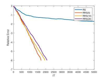
(a) $A\in\mathbb{R}^{3000\times 100}$

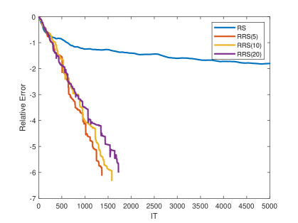
(b) $A\in\mathbb{R}^{100\times 3000}$

Figure 2: Convergence curves for overdetermined and underdetermined cases

From Figure 2, it is observed that the restarted randomized surrounding method converges with expected linear rate and the curves decrease much steeper than that of randomized surrounding method in both the underdetermined and overdetermined cases. It indicates that restarted randomized surrounding method is much efficient than the original randomized surrounding method for underdetermined and overdetermined cases.

In order to further compare the convergence performance, in Table 1 and Table 2, the number of iteration and the elapsed CPU time of randomized surrounding method and restarted randomized surrounding method for $q=5,10$ and $20$ are listed for different sizes respectively. All results are computed the average over 40 trials.

		$1000\times 100$	$2000\times 100$	$3000\times 100$	$4000\times 100$	$5000\times 100$
RS	IT	5000	5000	5000	5000	5000
	CPU	0.0088	0.0093	0.0100	0.0097	0.0107
RRS(5)	IT	1929	1830	1812	1804	1776
	CPU	0.0035	0.0036	0.0040	0.0039	0.0041
RRS(10)	IT	2062	1962	1952	1945	1950
	CPU	0.0036	0.0038	0.0050	0.0041	0.0044
RRS(20)	IT	2163	2092	2061	2064	2043
	CPU	0.0038	0.0041	0.0047	0.0043	0.0045

Table 1: Numerical results for overdetermined cases

		$100\times 1000$	$100\times 2000$	$100\times 3000$	$100\times 4000$	$100\times 5000$
RS	IT	5000	5000	5000	5000	5000
	CPU	0.0282	0.0584	0.1114	0.1847	0.3399
RRS(5)	IT	1729	1608	1541	1531	1472
	CPU	0.0093	0.0182	0.0331	0.0539	0.0922
RRS(10)	IT	1893	1740	1663	1672	1666
	CPU	0.0102	0.0194	0.0371	0.0596	0.1052
RRS(20)	IT	1978	1893	1805	1775	1741
	CPU	0.0106	0.0211	0.0404	0.0630	0.1112

Table 2: Numerical results for underdetermined cases

From Table 1 and Table 2, it is seen that the restarted randomized surrounding methods are efficient, and require less steps and CPU time than randomized surrounding method. Among these methods, the restarted randomized surrounding methods with $q=5$ performs the best, which indicates that a small number of restart may greatly improve the rate of convergence.

Example2. The test matrices are chosen from the SuiteSparse Matrix Collection. The property of the matrices including size, density, rank and Euclidean condition number (i.e., cond ) of the tested matrices are given in Table 3.

name	$crew1$	$bibd\_13\_6$	$cari$	$bibd\_16\_8$
size	$135\times 6469$	$78\times 1716$	$400\times 1200$	$120\times 12870$
rank	135	78	400	120
density	5.38%	19.23%	31.83%	23.33%
cond	18.20	6.27	3.13	9.54

Table 3: Information of the matrices from the Matrix Market

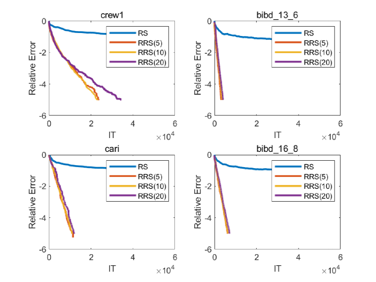
Figure 3: Convergence curves for the matrices from Matrix Market

The curves of the relative error versus the number of the iteration are plotted in Figure 3 for randomized surrounding method and restarted randomized surrounding methods respectively. From Figure 3, it is seen that all the restarted randomized surrounding methods converges faster than the randomized surrounding method, which further confirms the efficiency of the restart technique.

In Table 4, the number of iteration and the elapsed CPU time of the randomized surrounding method and restarted randomized surrounding methods when $q=5,10,20$ are listed respectively.

Method		$crew1$	$bibd\_13\_6$	$cari$	$bibd\_16\_8$
RS	IT	5000	5000	5000	5000
	CPU	22.3069	5.2526	4.2073	79.2887
RRS(5)	IT	11921	2027	6319	3592
	CPU	5.2916	0.2139	0.5388	5.5906
RRS(10)	IT	11545	2210	6901	3914
	CPU	5.0950	0.2319	0.5826	6.0782
RRS(20)	IT	11456	2399	7256	4304
	CPU	5.1426	0.2502	0.6167	6.6959

Table 4: Numerical results for the matrices from Matrix Market

From Table 4, it is seen that the restarted randomized surrounding methods are efficient, and require less number of iteration and CPU time than the randomized surrounding method. For the matrix ‘crew1’, RRS(10) require the least CPU time while RRS(20) take the least number of iteration; for the other three examples, RRS(5) require the least CPU time and the least number of iteration. This implies that the restarted strategy is efficient and can greatly improve the convergence while the optimal restart number is possibly problem depended.

Example 3. Finally, we compare these methods for solving a 2-D parallel-beam tomography problem and a seismic travel-time tomography problem generated by AIR tool box. The right term is $b=Ax_{\ast}+e$ where $e$ is the noise vector and the relative noise level is 0.01. The signal-noise ratio (SNR) is defined as

$$\text{SNR}:=10\log_{10}\frac{\sum_{i=0}^{n}x_{i}^{2}}{\sum_{i=0}^{n}(x_{i}-\hat{x}_{i})^{2}}$$

where $x$ is the original clean signal, $\hat{x}$ is the denoised signal, and $n$ is the length of the signal. The greater the value of SNR is, the better the denoising effect. The reconstruction images are compared in Figures 4 and 5 for a 2-D parallel-beam tomography problem and a seismic travel-time tomography problem respectively, after $100m$ iterations where $m$ is the number of rows.

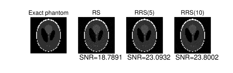
Figure 4: 2-D parallel-beam tomography problem where $A\in\mathbb{R}^{23883\times 2500}$

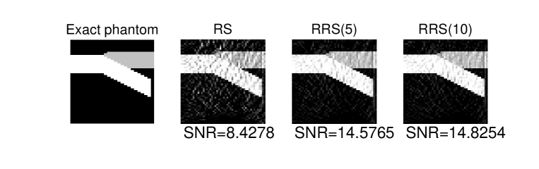
Figure 5: 2-D seismic travel-time tomography problem where $A\in\mathbb{R}^{2500\times 2500}$

From Figures 4 and 5, it is observed that the restarted randomized surrounding method can remove the noise and restore the real image efficiently. Moreover, the images reconstructed by the restarted randomized surrounding methods are better than that of the randomized surrounding method from the viewpoint of the sharpness of images and higher values of SNR. Among the three approaches, it is seen that the recovered image of RRS(10) is the best.

5 Conclusions

Restarted randomized surrounding methods are proposed for solving large linear problems. The convergence theory is established when the probability of row selection rule is proportional to the squared norm of row. Numerical experiments verify the proposed algorithms are efficient and outperform the existing method for overdetermined and underdetermined linear equations, as well as in the application in image processing. The continue work including of the dynamical restarted strategies, relaxation and the randomized selection rule are deserved to further study in the future.

References

- [1] Rainer Ansorge. Connections between the cimmino-method and the kaczmarz-method for the solution of singular and regular systems of equations. Computing, 33(3):367–375, 1984.
- [2] Mario Arioli, Iain S. Duff, Daniel Ruiz, and Miloud Sadkane. Block lanczos techniques for accelerating the block cimmino method. SIAM Journal on Scientific Computing, 16(6):1478–1511, 1995.
- [3] Zhong-Zhi Bai and Wen-Ting Wu. On greedy randomized kaczmarz method for solving large sparse linear systems. SIAM Journal on Scientific Computing, 40(1):A592–A606, 2018.
- [4] Zhong-Zhi Bai and Wen-Ting Wu. On partially randomized extended kaczmarz method for solving large sparse overdetermined inconsistent linear systems. Linear Algebra and Its Applications, 578:225–250, 2019.
- [5] Michele. Benzi. Gianfranco cimmino’s contributions to numerical mathematics. 2004.
- [6] Yair Censor. Row-action methods for huge and sparse systems and their applications. SIAM review, 23(4):444–466, 1981.
- [7] Gianfranco Cimmino. Cacolo approssimato per le soluzioni dei systemi di equazioni lineari. La Ricerca Scientifica (Roma), 1:326–333, 1938.
- [8] Yi-Shu Du, Ken Hayami, Ning Zheng, Keiichi Morikuni, and Jun-Feng Yin. Kaczmarz-type inner-iteration preconditioned flexible gmres methods for consistent linear systems. SIAM Journal on Scientific Computing, 43(5):S345–S366, 2021.
- [9] Tommy Elfving. Block-iterative methods for consistent and inconsistent linear equations. Numerische Mathematik, 35(1):1–12, 1980.
- [10] Xiang-Long Jiang, Ke Zhang, and Jun-Feng Yin. Randomized block kaczmarz methods with k-means clustering for solving large linear systems. Journal of Computational and Applied Mathematics, 403:113828, 2022.
- [11] Stefan Karczmarz. Angenaherte auflosung von systemen linearer glei-chungen. Bull. Int. Acad. Pol. Sic. Let., Cl. Sci. Math. Nat., pages 355–357, 1937.
- [12] Stefania Petra, Constantin Popa, and Christoph Schnörr. Extended and Constrained Cimmino-type Algorithms with Applications in Tomographic Image Reconstruction. Universitätsbibliothek Heidelberg, 2008.
- [13] Stefan Steinerberger. Surrounding the solution of a linear system of equations from all sides. Quart. Appl. Math., 79:419–429, 2021.
- [14] Thomas Strohmer and Roman Vershynin. A randomized Kaczmarz algorithm with exponential convergence. Journal of Fourier Analysis and Applications, 15(2):262–278, 2009.
- [15] F. Sukru Torun, Murat Manguoglu, and Cevdet Aykanat. A novel partitioning method for accelerating the block cimmino algorithm. SIAM Journal on Scientific Computing, 40(6):C827–C850, 2018.