A fast quantum algorithm for computing matrix permanent

Abstract

Computing a matrix permanent is known to be a classically intractable problem. This paper presents the first efficient quantum algorithm for computing matrix permanents. We transformed the well-known Ryser’s formula into a single quantum overlap integral and a polynomial sum of quantum overlap integrals to estimate a matrix permanent with the multiplicative error and additive error protocols, respectively. We show that the multiplicative error estimation of a matrix permanent would be possible for a special set of matrices. Such a quantum algorithm would imply that quantum computers can be more powerful than we expected. Depending on the size of a matrix norm and the ratio between 2-norm and 1-norm, we can obtain an exponentially small additive error estimation and better estimation against Gurvits’ classical sampling algorithm with our quantum protocol. Our quantum algorithm attains the milestone of opening a new direction in quantum computing and computational complexity theory. It might resolve crucial computational complexity issues like locating the bounded error quantum polynomial time (BQP) relative to the polynomial hierarchy, which has been a big complexity question. Moreover, our quantum algorithm directly shows the computational complexity connection between the matrix permanent and the real-time partition function of the quantum Ising Hamiltonian.

Almost three decades ago, Peter Shor [1] discovered a celebrated polynomial time quantum algorithm for integer factorisation. Although the best-known classical algorithm for integer factorisation scales quasi-exponentially, the problem’s computational complexity has not been settled yet. Therefore, we cannot claim quantum supremacy [2] clearly with Shor’s quantum algorithm. For factoring an $L$-bit number, it requires $\mathcal{O}(L)$ qubits and $\mathcal{O}(L^{3})$ quantum gate operations mainly for the quantum Fourier transform (QFT). The current classical factoring limit is about two thousand bits. Therefore, implementing Shor’s quantum algorithm for factoring large integer numbers requires a fault-tolerant error-correcting universal quantum computer, which cannot be built in the near term due to technical challenges. Nevertheless, we cannot show quantum supremacy with Grover’s search algorithm [3] because it can only achieve a quadratic speedup compared to the best-known classical algorithm. Consequently, other problems, which can provide clear computational complexity proofs and are implementable without expensive quantum subroutines like the QFT, are expected to demonstrate quantum computers’ computational superiority against their classical counterparts.

In this context, Aaronson and Arkhipov (AA) [4] suggested a quantum sampling problem [5, 2, 6], called boson sampling, that could potentially challenge the extended Church Turing thesis and demonstrate the quantum supremacy. The hardness of boson sampling is established on the computational complexity of matrix permanents. Approximating permanents of arbitrary complex or real square matrices with a constant factor is a #P-hard problem. Using two conjectures, namely, permanent of Gaussian conjecture (PGC) and permanent anti-concentration conjecture (PAC), AA showed an efficient classical simulation of boson sampling, i.e. an additive error matrix permanent estimator, would collapse the polynomial hierarchy (PH) to the third level; this is strongly believed not to happen. Specifically, the classical hardness of boson sampling relies on the hardness of the permanents of random complex Gaussian matrices. Nevertheless, the #P-hardness of permanents of Gaussian matrices has not yet been proved. The multiplicative error estimation of permanents of Gaussian matrices is conjectured as #P-hard in PGC. Assuming a non-uniform distribution of permanents of random Gaussian matrices by PAC, it was shown that the multiplicative error estimation is equivalent to the additive error estimation for the permanents of Gaussian matrices.

Similar complexity logics of boson sampling were applied to a quantum circuit model, instantaneous quantum polynomial time (IQP) problem [7]. The IQP circuit is composed of commuting gates. The resulting output qubit distribution cannot be efficiently determined using classical computers: the corresponding quantum overlap integrals can be interpreted as real-time partition functions of the quantum Ising Hamiltonian (Heisenberg model) [8, 9, 10]. Google research [11] demonstrated the quantum supremacy with the random circuit sampling problem using their 53-superconducting-qubit device by introducing non-commuting quantum gates, unlike the IQP setup. However, the verification and performance remain arguable [12, 13].

Regardless of these quantum sampling efforts, quantum algorithms for well-classified decision problems are needed for practical applications and quantum computational supremacy or advantage issues. The development of such quantum algorithms for decision problems can naturally lead to practical applications, unlike quantum sampling problems, cf. Refs. [14, 15]. Hopefully, we do not need to rely on the conjectures as to the sampling problems and the expensive QFT subroutine.

Troyansky and Tishby [16] showed how a Hermitian matrix permanent is expressed with an expectation value of a linear optical quantum observable. They concluded that exponentially many samples are needed to compute a permanent because the observable variance is significant. Note that the boson sampling device cannot be used to estimate permanents as the magnitudes are generally exponentially small. There are only a few efforts, as yet, to relate quantum circuit models to matrix permanents. Most of the studies focused on the computational hardness proof of computing permanents via the quantum circuit models [17, 18], which did not result in practical quantum algorithms for estimating matrix permanents.

It is believed, although without proof, that even quantum computers are not expected to access the #P-hard problem. Nevertheless, developing a quantum algorithm for approximating the matrix permanent is essential to locating bounded error quantum polynomial time (BQP) relative to the PH. The possible scenarios for quantum supremacy or quantum advantage would be the development of quantum algorithms with the polynomial time estimation or the subexponential time estimation of matrix permanents. To the best of our knowledge, no practical quantum algorithm has been reported for computing permanents yet.

We transformed the well-known classical algorithm, Ryser’s formula [19], computing an $N$-dimensional matrix permanent with an exponential cost $\mathcal{O}(N^{2}2^{N})$, to sums of $N$-th powers of a binary function. Without any approximations, the multiplicative error protocol is presented by using the linear combination of unitaries (LCU) technique [20, 21, 22] and the multiplicative error quantum amplitude estimation method of Aaronson and Rall (AR) [23]. We showed that the multiplicative error estimation is possible for permanents of a special set of matrices. This opens the possibility that quantum computers would access the #P-hard problem [4]; see Theorem 1 and Corollary 1.

Then, we reformulated the power expansion as an $N$-th derivative of the quantum Ising Hamiltonian propagator for the additive error estimation protocol. Consequently, we clearly showed how the boson sampling and the IQP problems are connected [8, 9, 10] via expressing the matrix permanent as a linear combination of the real-time partition functions of the Ising Hamiltonian. Using the quantum power method of Seki et al. [24], which exploits the finite difference scheme for the time derivatives, the matrix permanent estimation problem becomes an overlap integral evaluation problem. We propose an additive error protocol using the Hadamard test [25, 26] for the quantum overlap integral estimation. We compared our quantum algorithm to the best classical random sampling algorithm, i.e. the Gurvits algorithm [27, 4], and found criteria for the quantum advantage. Our additive error quantum protocol requires a polynomial number of quantum gates and depth, $\mathcal{O}(N^{2})$ for $2N+1$ qubits, that it is practically implementable in noisy intermediate-scale quantum (NISQ) devices.

Eventually, this paper presents the first efficient quantum algorithm for approximating matrix permanents with multiplicative error and additive error protocols. We also note that our quantum algorithm is potentially applicable to other matrix functions such as (loop)-hafnians [28, 29], Torontonians [30], determinants, and immanants, which are related to symmetries of quantum particles [31].

The rest of the paper is structured as follows: First, we transform the Ryser formula to a sum of $N$-th power of binary functions. A multiplicative error protocol with the LCU technique is discussed. Then, we show that a matrix permanent can be approximately cast into the sum of quantum overlap integrals. The additive error protocol is followed. Finally, after presenting quantum circuits for estimating a matrix permanent with an additive error using the Hadamard test, we discuss the implications of our findings and conclude the paper.

Results

Classical formulas

Recall the definition of permanent of a square matrix $A\in\mathbb{C}^{N\times N}$:

$$\mathrm{Per}(A)=\sum_{\vec{{\sigma}}\in S_{\mathrm{p}}}\prod_{j=1}^{N}A_{j,\sigma_{j}},$$ (1)

where $A_{jk}$ are the entries of $A$ and the set $S_{\mathrm{p}}$ includes all the permutations of $(1,2,\ldots,N)$, $\{\vec{\sigma}\}$ ($\vec{\sigma}=(\sigma_{1},\ldots\sigma_{N})$ is an $N$-dimensional vector). Brute force computation of a matrix permanent in Eq. (1) requires $N!$ terms in the summation, and each term is composed of products of $N$ elements of the matrix. In 1963, Ryser [19] discovered a formula for matrix permanent, which involves only $2^{N}$ terms in the summation,

$$\textrm{Per}(A)=(-1)^{N}\sum_{S\subseteq\{1,\ldots,N\}}(-1)^{|S|}\prod_{j=1}^{N}\sum_{k\in S}A_{jk},$$ (2)

where $|S|$ is the cardinality of subset $S$. Although, this is a dramatic improvement, the algorithm is still not classically efficient as it scales exponentially $\mathcal{O}(N^{2}2^{N})$. We can rewrite the Ryser formula (2) by introducing an $N$-dimensional binary vector $\vec{y}$ as follows:

$$\textrm{Per}(A)=\sum_{\vec{y}\in\{0,1\}^{N}}(-1)^{\sum_{k=1}^{N}(y_{k}+1)}\prod_{j=1}^{N}(\vec{A}_{j}\cdot\vec{y}),$$ (3)

where $\vec{A}_{j}$ is the $j$-th row of $A$. By introducing a variable $x_{k}=2y_{k}-1$, which maps from $\{0,1\}^{N}$ to $\{-1,1\}^{N}$, we can find the Glynn formula [32, 33, 34, 35]:

$$\textrm{Per}(A)=\frac{1}{2^{N}}\sum_{\vec{x}\in\{-1,1\}^{N}}\left(\prod_{k=1}^{N}x_{k}\right)\left(\prod_{j=1}^{N}\vec{A}_{j}\cdot\vec{x}\right),$$ (4)

where we used the identity $\sum_{\vec{x}\in\{-1,1\}^{N}}\prod_{k}^{N}x_{k}=0$. Eq. 4 shows the magnitude is bounded by $\|A\|^{N}$. Gurvits [27, 4] suggested an additive error algorithm $\pm\epsilon\|A\|^{N}$ based on Glynn’s formula by interpreting it as an expectation value $E(\prod_{k=1}^{N}x_{k}\prod_{j=1}^{N}\vec{A}_{j}\cdot\vec{x})$ over the random binary vector $\vec{x}$. $\|\cdot\|$ is the matrix 2-norm; otherwise, the order is indicated.

Using the identity of a monomial by Kan [28], we have

$$\prod_{j=1}^{N}\vec{A}_{j}\cdot\vec{x}=\frac{1}{N!2^{N}}\sum_{\vec{x}^{\prime}\in\{-1,1\}^{N}}\left(\prod_{k=1}^{N}x^{\prime}_{k}\right)\left(\vec{x^{\prime}}^{\top}A\vec{x}\right)^{N}.$$ (5)

Now, we have a new expression for the matrix permanent by inserting Eq. (5) into Eq. (4) as follows:

$$\mathrm{Per}(A)=\frac{1}{N!2^{2N}}\sum_{\vec{x},\vec{x^{\prime}}\in\{-1,1\}^{N}}\left(\prod_{k=1}^{N}x_{k}x_{k}^{\prime}\right)\left(\vec{x^{\prime}}^{\top}A\vec{x}\right)^{N},$$ (6)

whose magnitude is bounded by $(\sum_{j,k}|A_{jk}|)^{N}/N!$.

We name our new finding in Eq. (6) the Glynn-Kan formula in this paper. Thus, Per($A$) can be interpreted as an average of $2^{2N}$ $N$-th power of binary functions by Eq. (6).

At a glance, our new formula for permanents in Eq. (6) is exponentially more inefficient compared with the original Ryser’s formula, Eq. (2). However, our new formula is suitable for developing a BQP quantum algorithm for permanents because they are composed of an expectation value of $N$-th powers of the binary function, i.e. $\vec{x^{\prime}}^{\top}A\vec{x}$. We use these formulas to develop quantum algorithms for estimating the permanents of arbitrary square matrices. In the following section, we develop quantum algorithms for multiplicative error and additive error approximation of matrix permanents.

Quantum algorithm

From the Glynn-Kan formula in Eq. (6), we immediately identify the following quantum expectation value as a matrix permanent:

$$\textrm{Per}(A)=$$

$$\tfrac{1}{N!2^{2N}}\sum_{y=0}^{2^{2N}-1}\langle y|\left(\bigotimes_{k=1}^{N}Z_{k}Z_{N+k}\right)\left(\sum_{j,k=1}^{N}A_{jk}Z_{N+j}Z_{k}\right)^{N}|y\rangle,$$ (7)

where $|y\rangle=|y_{1}\rangle\cdots|y_{2N}\rangle$, $y=y_{1}\cdots y_{2N}$ is given as a $2N$-bit string and $Z_{k}$ is a Pauli-Z operator on the $k$-th qubit. Using the identity, $\frac{1}{2^{N}}\sum_{y=0}^{2^{2N}-1}|y\rangle=\bigotimes_{k=1}^{2N}H_{k}|0\cdots 0\rangle=|\phi\rangle$, where $H_{k}$ is a Hadamard operator of the $k$-th qubit, we rewrite the matrix permanent as an expectation value of a quantum operator, i.e. $\mathrm{Per}(A)=\frac{1}{N!2^{2N}}\mathrm{Tr}[G(A)]=\frac{1}{N!}\langle\phi|G(A)|\phi\rangle$. Let us call $G(A)$ the Glynn-Kan operator, defined as

$$G(A)=\left(\bigotimes_{k=1}^{N}Z_{k}Z_{N+k}\right)\left(\sum_{j,k=1}^{N}A_{jk}Z_{N+j}Z_{k}\right)^{N},$$ (8)

which is factored with two components–parity operator and Ising operator, respectively denoted as $P$ and $\mathcal{H}$. That is, $G(A)=P\mathcal{H}^{N}(A)$, where $\mathcal{H}(A)=\sum_{j,k=1}^{N}A_{jk}Z_{N+j}Z_{k}$ and $P=\bigotimes_{k=1}^{N}Z_{k}Z_{N+k}$. Thus far, we have expressed the matrix permanent as an expectation value of qubit operators and qubit states. The resulting expression involves a power operator of $\mathcal{H}$, which is non-unitary and generally non-Hermitian. The remaining task is to approximately implement the power operator in a quantum circuit. We can perform the approximation through different approaches. For example, we can consider quantum signal processing with quantum singular value transformation and the LCU technique [20, 21, 22]. However, the repeated application of LCU for the power operator requires many ancilla qubits, and the success rate scales badly.

Multiplicative error protocol

Nevertheless, besides the practicality, let’s discuss the possibility of multiplicative error estimation of matrix permanent with the Glynn-Kan operator (8) before we present the realistically implementable additive error quantum protocol. The multiplicative error estimation of magnitudes of matrix permanents would be possible for a special set of matrices according to the following theorem:

Theorem 1

For a given matrix $A\in\mathbb{C}^{N\times N}$, if $|\mathrm{Per}(A)|\geq\beta\geq 0$, and $\beta\leq\|\mathcal{H}(A)\|^{N}/N!\leq\mathrm{poly}(N)\beta$, then a BQP machine can efficiently estimate $|\mathrm{Per}(A)|$ with a multiplicative error.

Proof. Using the LCU technique [20, 21, 22], $\mathcal{H}(A)$ can be expressed as a quantum overlap integral, i.e., $\mathcal{H}(A)=\|\mathcal{H}(A)\|\braket{\phi^{(c)}}{W^{(c)}}{\phi^{(c)}}$, where $W^{(c)}$ and $\ket{\phi^{(c)}}$ are the controlled-unitaries and the ancilla state with $2\log_{2}N$ ancilla qubits. Therefore, the magnitude of a matrix permanent can be expressed with a single quantum amplitude, according to the Glynn-Kan operator (8):

$$|\mathrm{Per}(A)|=\frac{\|\mathcal{H}(A)\|^{N}}{N!}a,$$ (9)

where $a$ is the quantum amplitude of $2N\log_{2}2N$ qubits ($2N$ system qubits and $N\times 2\log_{2}N$ ancilla qubits) and $\|\mathcal{H}(A)\|=\sum_{j,k}|A_{jk}|$. Eq. (9) obviously tells the magnitude upper bound of a matrix permanent is $\|\mathcal{H}(A)\|^{N}/N!$ as in Eq. (6) because $0\leq a\leq 1$. Since the magnitude of the permanent is given as a single quantum amplitude, the multiplicative error estimation of the amplitude results in the BQP estimation of the magnitude of the matrix permanent with a multiplicative error. For the multiplicative error BQP estimation of a quantum amplitude $a$, $a$ has to be polynomially small ($1/\mathrm{poly}(N)$) to use the AR amplitude estimation algorithm [23]. The amplitude can be obtained within the multiplicative error factors ($1\pm\epsilon$) by querying the Grover diffusion operator $\mathcal{O}(1/(\epsilon a))$ times. Here, we consider conditions of the polynomially small $a$ value for the polynomial number of queries.

If the magnitude of the permanent has a lower bound $\beta$, the lower bound of $a$, which is polynomially small, is given as follows:

$$a\geq\frac{\beta N!}{\|\mathcal{H}(A)\|^{N}}\geq\frac{1}{\mathrm{poly}(N)}.$$ (10)

Finally, we have a bound condition of $\|\mathcal{H}(A)\|$ as $\beta\leq\|\mathcal{H}(A)\|^{N}/N!\leq\mathrm{poly}(N)\beta$. Here, we note that if we allow $a$ to be subexponentially small, then we can estimate the matrix permanent with a multiplicative error in a subexponential time, which has not been achieved by classical algorithms yet.

Corollary 1

For a given matrix $A\in\mathbb{C}^{N\times N}$, with conditions of $|\mathrm{Per}(A)|\geq\beta\geq 0$, and $\beta\leq\|\mathcal{H}(A)\|^{N}/N!\leq\mathrm{poly}(N)\beta$, if the multiplicative error estimation of $|\mathrm{Per}(A)|$ is a #P-hard problem, then $\mathrm{BQP=P^{\#P}}$ according to Theorem 1.

Proof. If the matrix $A$ satisfies the conditions in the corollary, the BQP machine can estimate the magnitude of the matrix permanent with a multiplicative error according to Theorem 1. Though the multiplicative error estimation of the magnitude of a permanent of an arbitrary matrix is known to be a #P-hard problem, the complexity of $|\mathrm{Per}(A)|$ is not known. Therefore, if the multiplicative error estimation of $|\mathrm{Per}(A)|$ is a #P-hard problem, then $\mathrm{BQP=P^{\#P}}$.

Additive error protocol

In this paper, we adopt the approach of Seki et al. [24], the quantum power method, a quantum version of the finite difference method for time-derivatives of a quantum propagator, because it results in simpler quantum circuits. In this section, we mainly focus on real matrices for simplicity. It is straightforward to apply the method and the error analysis for complex matrices, which can be found in the methods section.

Unitary approximation

When $A$ is a real matrix, i.e. $A=B$, $\mathcal{H}(B)$ is a Hermitian operator that we can express the power operator as the time derivatives of the corresponding time propagator $U(B;t)=\exp(-\mathrm{i}\mathcal{H}(B)t)$ directly as

$$\mathcal{H}(B)^{N}=\mathrm{i}^{N}\frac{\partial^{N}U(B;t)}{\partial t^{N}}\Big{|}_{t=0}.$$ (11)

We can approximately implement the time derivatives using the finite difference method, as follows, with the time step $\Delta t$,

$$\frac{\mathrm{i}^{N}}{\Delta t^{N}}\left[U\left(B;\Delta t/2\right)-U\left(B;-\Delta t/2\right)\right]^{N}$$

$$=\frac{\mathrm{i}^{N}}{\Delta t^{N}}\sum_{l=0}^{N}(-1)^{l}\binom{N}{l}U\left((N-2l)B;\Delta t/2\right)$$ (12)

$$=\mathcal{H}(B)^{N}-\frac{N\Delta t^{2}}{24}\mathcal{H}(B)^{N+2}+\cdots,$$ (13)

where $\|\mathcal{H}(B)\|\Delta t/2\leq 1$ is the convergence condition for the expansion. Thus, the Glynn-Kan operator is approximately given as a linear combination of unitary gates as follows:

$$G(B)\simeq\frac{(-1)^{N}}{\Delta t^{N}}\sum_{l=0}^{N}(-1)^{l}\binom{N}{l}U\left(B^{(l)};\Delta t/2\right),$$ (14)

where $B^{(l)}=(N-2l)B+\pi\Delta t^{-1}I$ and $I$ is an identity matrix. We used the following identity for the parity operator, $P=\mathrm{i}^{N}\bigotimes_{k=1}^{N}\exp\left(-\frac{\pi}{2}\mathrm{i}Z_{k}Z_{N+k}\right)$, to hide it in the unitary propagator $U$. By hiding the parity operator, we can simplify the required quantum circuits. Finally, the permanent of the real matrix $B$ is approximated as the sum of $N+1$ quantum overlap integrals,

$$\mathrm{Per}(B)= \frac{(-1)^{N}}{N!\Delta t^{N}}\sum_{l=0}^{N}(-1)^{l}\binom{N}{l}\braket{\phi}{U\left(B^{(l)};\Delta t/2\right)}{\phi}$$

$$+\mathcal{O}(\frac{N\Delta t^{2}}{24N!}\|\mathcal{H}(B)\|^{N+2}).$$ (15)

For the quantum algorithm’s practical application, we can systematically improve the error introduced by the finite difference with the Richardson extrapolation method [24] for the given time step $\Delta t$. Eq. (15) can be further simplified using the time reversal symmetry, $[\mathrm{i}^{N}U(-\Delta t/2)]=[\mathrm{i}^{N}U(\Delta t/2)]^{{}^{\dagger}}$. We only need to estimate a half ($\left\lfloor(N+1)/2\right\rfloor$) of the real parts of the quantum overlap integrals, respectively, as follows:

$$\mathrm{Per}(B)\simeq$$

$$\frac{2(-1)^{N}}{N!\Delta t^{N}}\sum_{l=0}^{\left\lfloor\tfrac{N-1}{2}\right\rfloor}(-1)^{l}\binom{N}{l}\mathrm{Re}\braket{\phi}{U\left(B^{(l)};\Delta t/2\right)}{\phi}.$$ (16)

Error analysis

Now the matrix permanent estimation problem becomes the evaluation problem of the real part of the quantum overlap integral, i.e. $\mathrm{Re}\braket{\phi}{U}{\phi}$, for both real and complex matrices. Here, we propose an additive error protocol, which can be implemented in simpler quantum circuits and is suitable for NISQ devices. We can obtain the real parts of quantum overlap integrals via the ancilla qubit measurement of the Hadamard test  [25, 26] in Fig. 2(a).

The number of samplings for each real part is $\mathcal{O}\left(\epsilon_{\mathrm{HT}}^{-2}\log(1/\delta)\right)$, where $\epsilon_{\mathrm{HT}}$ and $\delta$ are the required precision and a failure probability of the Hadamard test [25, 8, 36], respectively. The errors in our quantum algorithm are caused by the finite difference method for the differentiation and the Hadamard test for the quantum overlap integral additive error estimation. In the following, we analyse the additive errors for real matrices compared with the Gurvits classical sampling algorithm. The error analyses of complex matrices and random Gaussian matrices are presented in the methods section. The total additive error of a real matrix permanent $\epsilon_{\mathrm{Tot}}$ has an upper bound as follows:

$$\epsilon_{\mathrm{Tot}} \leq\frac{1}{N!}\left(\epsilon_{\mathrm{HT}}\left(\frac{2}{\Delta t}\right)^{N}+\epsilon_{\mathrm{FD}}\frac{N\Delta t^{2}}{24}\|\mathcal{H}(B)\|^{N+2}\right),$$ (17)

where $0<\epsilon_{\mathrm{HT}}$, $\epsilon_{\mathrm{FD}}=1/\mathrm{poly}(N)<1$. Here, $\epsilon_{\mathrm{HT}}$ and $\epsilon_{\mathrm{FD}}$ are constant error factors caused by the Hadamard test and the finite difference method, respectively, and we used the following identity, $\tfrac{1}{\Delta t^{N}}\sum_{l=0}^{N}\binom{N}{l}=\left(\frac{2}{\Delta t}\right)^{N}$. Note that the upper bound is set for the worst-case scenario, although we expect that the error cancellation can occur among the additive errors having different signs. Using the upper bound of the inverse factorial, $\frac{1}{N!}<\frac{1}{\sqrt{2\pi N}}\left(\frac{e}{N}\right)^{N}$, we found an upper bound of the additive error expressed with powers,

$$\epsilon_{\mathrm{Tot}}\leq \frac{1}{\sqrt{2\pi N}}\left(\frac{2e}{N\Delta t}\right)^{N}$$

$$\left(\epsilon_{\mathrm{HT}}+\frac{\epsilon_{\mathrm{FD}}N}{6}\left(\frac{\|\mathcal{H}(B)\|\Delta t}{2}\right)^{N+2}\right).$$ (18)

Because of the convergence condition, we have

$$\epsilon_{\mathrm{Tot}}\leq\epsilon_{\mathrm{R}}\left(\frac{2e}{N\Delta t}\right)^{N},$$ (19)

where $\epsilon_{\mathrm{R}}=(\epsilon_{\mathrm{HT}}+\epsilon_{\mathrm{FD}}N/6)/\sqrt{2\pi N}$.

Using the upper bound of the total error, we can achieve an exponentially small additive error with the following condition:

$$\frac{2e}{N}<\Delta t\leq\frac{2}{\|\mathcal{H}(B)\|}.$$ (20)

Gurvits’ classical sampling algorithm can estimate a matrix permanent with an additive error $\epsilon\|A\|^{N}$, where $0<\epsilon=1/\mathrm{poly}(N)<1$. It can produce exponentially small, polynomially small, or exponentially large errors depending on the size of the matrix spectral norm. Here, we test our quantum algorithm against Gurvits’ classical sampling algorithm, considering what condition can yield a better additive error. Without loss of generality, we consider complex matrices here because the real matrices carry identical bound conditions as the complex matrices.

We devise an inequality using Eq. (37) and Gurvits’ additive error to find a condition for the superiority of our quantum algorithm, i.e.

$$\epsilon\left(\frac{de}{N\Delta t}\right)^{N}\leq\epsilon\|A\|^{N},$$ (21)

where $d$ is identified as 2 or 4, respectively, for real or complex matrices, and we set $0<\epsilon_{\mathrm{C}}=\epsilon<1$. The resulting bound for $\Delta t$ is given as follows:

$$\frac{de}{N\|A\|}\leq\Delta t\leq\frac{d}{\|\mathcal{H}(A)\|}.$$ (22)

Thus, we have a condition for the superiority of our quantum algorithm with respect to the Gurvits algorithm as

$$\|\mathcal{H}(A)\|\leq\frac{N}{e}\|A\|.$$ (23)

Based on this condition (23), we may consider three cases:

1. $\|\mathcal{H}(A)\|\leq\frac{N}{e}\|A\|\leq\frac{N}{e}$, which implies $\|A\|\leq 1$: We can obtain exponentially small errors, smaller than Gurvits’ exponentially small error.

2. $\|\mathcal{H}(A)\|\leq\frac{N}{e}\leq\frac{N}{e}\|A\|$, which implies $\|A\|\geq 1$: We can still obtain exponentially small errors, but the Gurvits algorithm produces an exponentially large error.

3. $\frac{N}{e}\leq\|\mathcal{H}(A)\|\leq\frac{N}{e}\|A\|$, which implies $\|A\|\geq 1$: Both of our quantum algorithm and Gurvits’ classical algorithm produce an exponentially large error, but our quantum algorithm’s error is smaller than the classical one.

The quantum algorithm can perform exponentially better than its classical counterpart if the condition in Eq. (23) is satisfied. Here, we emphasise that case 2 above shows a domain where the quantum algorithm produces an exponentially small error, whereas the classical algorithm carries an exponentially large error. Now, let us see what Eq. (23) means. We know the Hamiltonian norm is upper-bounded by the 1-norm as

$$\|\mathcal{H}(A)\|\leq N\|A\|_{1}\leq\frac{N}{e}\|A\|,$$ (24)

where we set the upper bound, as in Eq. (23), to find a sufficient condition of matrix norms. Recalling the well-known inequality, $1/\sqrt{N}\leq\|A\|/\|A\|_{1}\leq\sqrt{N}$, we have

$$e\leq\frac{\|A\|}{\|A\|_{1}}\leq\sqrt{N},$$ (25)

which implies $e^{2}\leq N$. We observe that the domain in Eq. (25) is non-empty for the sufficiently large $N\geq 8$. Let us call it the quantum advantage domain. As obviously shown in the bound condition in Eq. (25), the quantum advantage domain becomes dominant as the matrix size increases and becomes larger than 50 % for $N\geq 28$; see Fig. 1.

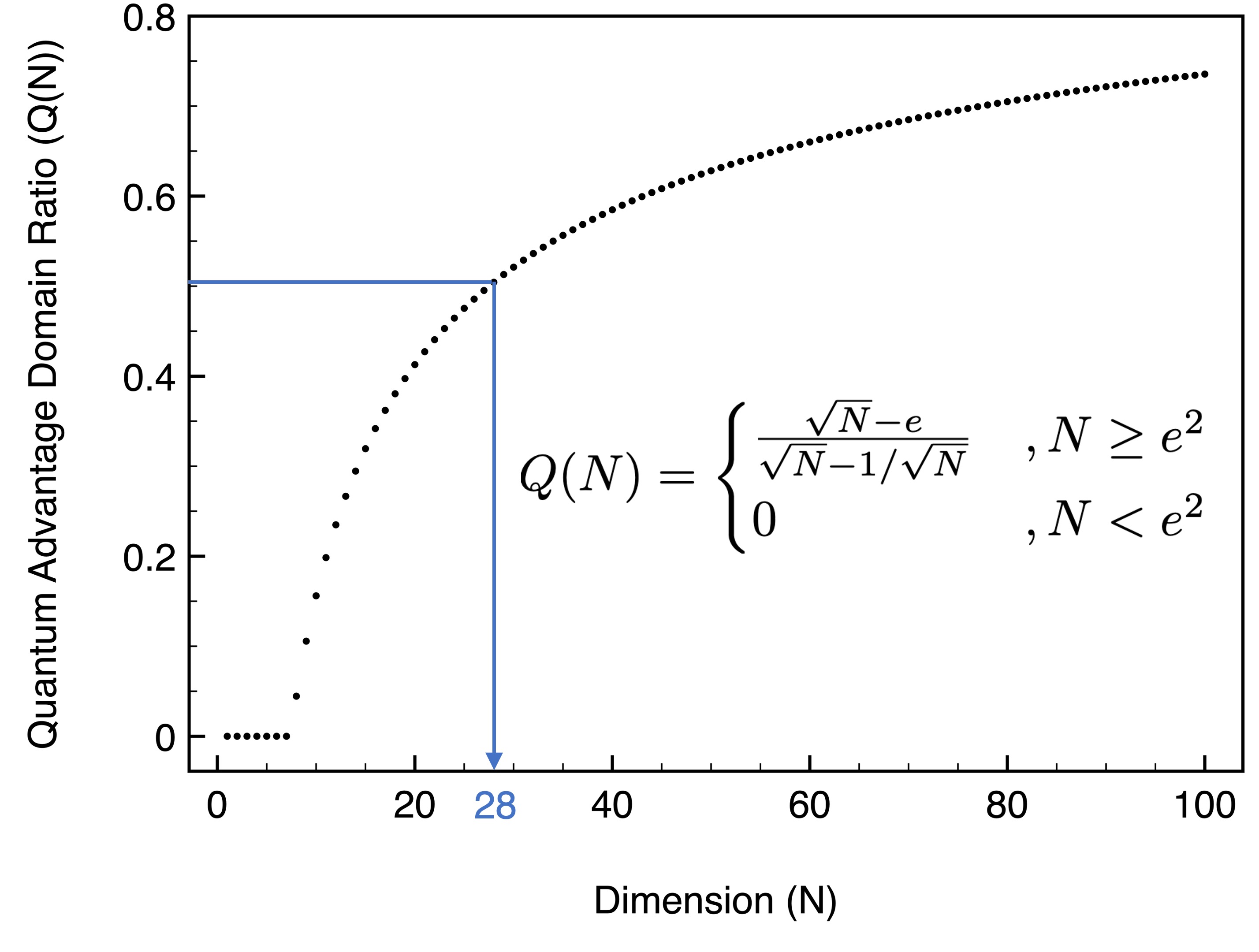
Figure 1: Quantum advantage domain ratio ($Q(N)$) in Eq. (25).

Figure 2: Quantum circuits for evaluating a real part of the overlap integral using the Hadamard test. (a) The Hadamard test circuit for the additive error ($1/\mathrm{poly(N)}$) estimation of the real part of the quantum overlap integral $\mathrm{Re}\braket{\phi}{U}{\phi}$. The real part of the quantum overlap integral can be obtained via the difference between the probabilities of getting $0$ and $1$ in the ancilla qubit (denoted as $c$) measurement. The detailed quantum circuit implementation is presented: (b) the circuit synthesis of the controlled-$R_{ZZ}(\theta)=\exp(-\mathrm{i}\tfrac{\theta}{2}Z_{1}Z_{2})$ gate and (c) the circuit synthesis of controlled-$R_{Z}(\theta)$, where $R_{Z}(\theta)=\exp(-\mathrm{i}\tfrac{\theta}{2}Z)$.

	Real matrix	Complex matrix
Number of $\mathrm{Re}\braket{\phi}{U}{\phi}$ to be evaluated	$\left\lfloor\frac{N+1}{2}\right\rfloor$	Odd $N$: $(N^{3}+6N^{2}+11N+6)/12$ Even $N$: $(N^{3}+6N^{2}+8N)/12$
Required number of qubits per $\mathrm{Re}\braket{\phi}{U}{\phi}$ estimation	$2N+1$	$2N+1$
Number of CNOT gates per $\mathrm{Re}\braket{\phi}{U}{\phi}$ estimation	$4N^{2}+2N$	$4N^{2}+2N$
Circuit depth per $\mathrm{Re}\braket{\phi}{U}{\phi}$ estimation	$9N^{2}+1$	$9N^{2}+1$
Total number of samples for estimating a permanent with the Hadamard test	$\mathcal{O}\left(\frac{N}{\epsilon_{\mathrm{HT}}^{2}}\log(\frac{1}{\delta})\right)$	$\mathcal{O}\left(\frac{N^{3}}{\epsilon_{\mathrm{HT}}^{2}}\log(\frac{1}{\delta})\right)$
Total error upper bound	$\epsilon\left(\frac{2e}{N\Delta t}\right)^{N}$	$\epsilon\left(\frac{4e}{N\Delta t}\right)^{N}$
$\Delta t$ for exponentially small additive error estimation	$\frac{2e}{N}<\Delta t<\frac{2}{\|\mathcal{H}(B)\|}$	$\frac{4e}{N}<\Delta t<\frac{4}{\|\mathcal{H}(A)\|}$
Sufficient condition for beating the Gurvits algorithm	$e\leq\frac{\|B\|}{\|B\|_{1}}\leq\sqrt{N}$	$e\leq\frac{\|A\|}{\|A\|_{1}}\leq\sqrt{N}$

Table 1: Summary of the additive error estimation protocol.

Here, we present the quantum circuit synthesis for the additive error protocol based on the Hadamard test for the practical application of our quantum algorithm in NISQ devices. Without loss of generality, we present the quantum circuit for real matrices; for the complex matrix case, we can simply use $A^{(l,j,k)}$, which is defined in the methods section, for the circuit synthesis instead of $B^{(l)}$. The time-propagator can be factorised into two-qubit gates as

$$U(B^{(l)};\Delta t/2)=\prod_{p,q=1}^{N}\exp\left(-\mathrm{i}B_{pq}^{(l)}\frac{\Delta t}{2}Z_{N+p}Z_{q}\right),$$ (26)

where the two-qubit gate is a simple Ising $ZZ$-gate $R_{ZZ}^{(p,q)}(\theta_{pq})=\exp(-\mathrm{i}\tfrac{\theta_{pq}}{2}Z_{N+p}Z_{q})$. We estimate the overlap integrals using the Hadamard test method in Fig. 2(a), and the required controlled-$U$ gate, $V$, is decomposed as a simple product of controlled-$R_{ZZ}$ gates as

$$V(B^{(l)};\Delta t/2)=$$

$$\prod_{p,q=1}^{N}(\ket{0^{(c)}}\bra{0^{(c)}}+\ket{1^{(c)}}\bra{1^{(c)}}\otimes R_{ZZ}^{(p,q)}(B_{pq}^{(l)}\Delta t)),$$ (27)

where $(c)$ denotes the control ancilla qubit. Accordingly, Fig. 2(a) shows the detailed quantum circuit corresponding to the Hadamard test. After all, we need to evaluate $\mathcal{O}(N)$ and $\mathcal{O}(N^{3})$ real part of the overlap integrals to estimate the permanents of real and complex matrices, respectively. In any case, it requires $2N+1$ qubits with $\mathcal{O}(N^{2})$ circuit depth and CNOT gates per single overlap integral evaluation. Tab. 1 summarises the additive error protocol.

Discussion

This paper reported a new classical formula for matrix permanent named the Glynn-Kan formula, which was discovered by introducing the monomial expansion of Kan [28] to the Glynn formula [32]. Although the Glynn-Kan formula is exponentially more inefficient than Ryser’s formula, it has a simple structure of the $N$-th power of binary functions. It would be worth exploring to the study of the computational complexity of the permanents of various matrices using the Glynn-Kan formula. For example, the multiplicative error estimations of a matrix having 0-1 entries and the Hermitian positive semidefinite matrix are known to be obtainable in polynomial times. The Glynn-Kan formula would help develop the $\mathrm{BPP^{NP}}$ algorithm for the Hermitian positive semidefinite matrix. It is worth mentioning that the Glynn-Kan formula can be generalized for matrices with repeated rows and columns [33, 34, 35] and can be used to develop the corresponding quantum algorithms.

By converting the classical Glynn-Kan formula to the quantum expectation value of the Glynn-Kan operator, we developed quantum algorithms for computing matrix permanents for the first time. The possible multiplicative error estimation with the LCU technique and the AR method was discussed in Theorem 1 and Corollary 1. We showed that the multiplicative error estimation of permanents would be possible in some cases. Because the multiplicative error estimation of matrix permanent is known to be a #P-hard problem, the implication of our finding is remarkable. Although the quantum accessibility to the #P-hard problem is strongly believed to be impossible [4], the possibility is still open. So far, it has been shown by Lloyd et al.  [37] that it requires nonlinearity for a quantum device to access a #P-hard problem efficiently. Our multiplicative error quantum algorithm provides additional evidence to Refs. [38, 39, 40] that the BQP has capabilities beyond the PH. This paper proposes to show how we would be able to adequately locate the BQP concerning the PH using quantum algorithms for computing matrix permanents.

Using the finite difference method [24], we then approximated the quantum expectation value as the sum of the quantum overlap integrals. Consequently, the matrix permanent evaluation problem becomes a quantum overlap integral evaluation problem. We proposed an additive error quantum protocol for computing matrix permanents through the setup. Compared to the multiplicative error protocol, this algorithm can be practically implementable in NISQ devices. It requires $2N+1$ qubits and $4N^{2}+2N$ CNOT gates per single overlap integral evaluation of its real part. Interestingly, the required circuit complexities of the real and complex matrices are not different; only the required numbers of overlap integral evaluations are different. The additive error quantum protocol is comparable with the Gurvits classical sampling algorithm. We found a quantum advantage domain of the matrix norm where the quantum algorithm can provide a better estimation than the classical one. When the system size is sufficiently large ($\geq 28$), we expect the quantum advantage domain to be more than 50 %. However, here we note that the current additive error quantum protocol based on the Hadamard test has no chance of satisfying the requirement for the #P-hardness, unlike the multiplicative error protocol; see the methods section.

We provide a new tool to investigate computational complexity questions about the relationships among the BPP, BQP, and #P. We believe that our new findings in classical and quantum algorithms for computing matrix permanents would play an essential role in identifying the unclear relationship between the BQP and PH. It is known so far only that $\mathrm{BQP\subseteq P^{\#P}=P^{PP}}$ [41]. Hence, thorough computational complexity analyses are anticipated in subsequent studies.

Lastly, we note that our quantum algorithm can be used for the boson sampling [42], and interestingly, it directly connects the boson sampling and the IQP to approximate matrix permanents as a linear combination of the real-time partition function of quantum Ising Hamiltonian [8, 9, 10]. The circuit complexity differs depending on the quantum Ising Hamiltonian’s matrix elements since different matrices would give different circuit complexities. Therefore, the quantum circuit model can analyse the computational complexity of a matrix permanent. Further investigations of the connection between boson sampling and qubit sampling (IQP) should be explored.

Our quantum algorithm for computing matrix permanent attained a milestone in the quantum computing and the computational complexity theory and opened new computational complexity questions. It could be used to answer those questions by itself. Our quantum algorithm can be modified to compute other matrix functions like (loop)-hafnians, Torontonians, determinants, and immanants with minor changes; the related works will appear elsewhere soon. The subsequent paper will explore various numerical procedures, including the Gaussian process and interpolation techniques, applying our additive error quantum algorithm using cloud quantum computers like IBM Quantum and IonQ. With the help of our findings, we believe that the BQP would serve as an essential bridge in answering the Millennium question $\mathrm{P}=\mathrm{NP}$ by adequately positioning BPP, BQP, and #P complexity classes.

Methods

Classical implication of of the Glynn-Kan formula (Eq. (6))

Interestingly, Eq. (6) can be rewritten as a difference between two positive semidefinite functions for a real square matrix of $B$ with an even dimension,

$$\mathrm{Per}(B)= \frac{1}{N!2^{2N}}\Huge[\sum_{\{\vec{x},\vec{x^{\prime}}\}\in\{-1,1\}^{N}}\mathcal{S}_{+}\left(\vec{x^{\prime}}^{\top}B\vec{x}\right)^{N}$$

$$-\sum_{\{\vec{x},\vec{x^{\prime}}\}\in\{-1,1\}^{N}}\mathcal{S}_{-}\left(\vec{x^{\prime}}^{\top}B\vec{x}\right)^{N}\Huge],$$ (28)

where $\mathcal{S}_{\pm}$ refers to $\left(\prod_{k=1}^{N}x_{k}\pm\prod_{k=1}^{N}x_{k}^{\prime}\right)^{2}/4$, respectively. For the odd-dimensional case, we can use the following identity to have the even-dimensional matrix, $\mathrm{Per}(B)=\mathrm{Per}\left(B\bigoplus 1\right)$. Eq. (28) directly shows #P-hard is GapP-hard by the definition of GapP [6]. On the other hand, the multiplicative error estimation of a permanent of a real matrix is also #P-hard. The positive semidefinite functions in Eq. (28) can be evaluated with multiplicative error estimation using Stockmeyer’s BPP^NP counting algorithm [4, 43], where BPP and NP stand for bounded error probabilistic polynomial time and nondeterministic polynomial time, respectively.

Meanwhile, the multiplicative error estimation of the permanent of a Hermitian positive semidefinite matrix is classified as $\mathrm{BPP^{NP}}$ [44, 45, 46]. Although it is known that permanents of non-negative matrices can be evaluated within a constant factor by Jerrum-Sinclair-Vigoda (JSV) algorithm [47] in polynomial time, the JSV algorithm has no practical implementations so far [48, 49]. Therefore, further computational complexity analysis of estimating permanents of real matrices using Eq. (28) is required. We would be able to discover new efficient classical algorithms with the Glynn-Kan formula.

Permanent formulas for complex matrix

When $A$ is a complex matrix, i.e. $A=B+\mathrm{i}C$, where $B$ and $C$ are real square matrices, we can expand Eq. (6) as follows:

$$\mathrm{Per}(A)=\frac{1}{N!2^{2N}}\sum_{l=0}^{N}\mathrm{i}^{l}\begin{pmatrix}N\\ l\end{pmatrix}$$

$$\sum_{\vec{x},\vec{x^{\prime}}\in\{-1,1\}^{N}}\left(\prod_{k=1}^{N}x_{k}x_{k}^{\prime}\right)\left(\vec{x^{\prime}}^{\top}B\vec{x}\right)^{N-l}\left(\vec{x^{\prime}}^{\top}C\vec{x}\right)^{l}.$$ (29)

The exact evaluation of Eq. (29) for the permanent of a complex matrix requires the summation of $(N+1)2^{2N}$ real binary functions with complex weights.

We exploit the classical expression in Eq. (29) for the quantum version as follows:

$$\mathrm{Per}(A)$$

$$=\frac{1}{N!}\sum_{l=0}^{N}\mathrm{i}^{l}\begin{pmatrix}N\\ l\end{pmatrix}\braket{\phi}{P\mathcal{H}^{N-l}(B)\mathcal{H}^{l}(C)}{\phi}$$ (30)

$$=\frac{(-1)^{N}}{N!\Delta t^{N}}\sum_{l=0}^{N}\sum_{j=0}^{N-l}\sum_{k=0}^{l}\mathrm{i}^{l}(-1)^{j+k}\binom{N}{l}\binom{N-l}{j}\binom{l}{k}$$

$$~{}~{}~{}~{}~{}~{}~{}~{}~{}~{}~{}~{}~{}~{}~{}~{}~{}~{}~{}~{}~{}~{}~{}~{}~{}~{}~{}~{}~{}\braket{\phi}{U(A^{(l,j,k)};\Delta t/2)}{\phi}$$

$$+\mathcal{O}\left(\frac{N\Delta t^{2}}{24N!}\|\mathcal{H}(A)\|^{N-1}(\|\mathcal{H}(B)\|^{3}+\|\mathcal{H}(C)\|^{3})\right),$$ (31)

where $A^{(l,j,k)}=(N-l-2j)B+(l-2k)C+\pi\Delta t^{-1}I$; we used the following expansion:

$$\frac{\mathrm{i}^{N}}{\Delta t^{N}}\Huge[U\left(B;\frac{\Delta t}{2}\right)-U\left(B;-\frac{\Delta t}{2}\right)$$

$$+\mathrm{i}\left(U\left(C;\frac{\Delta t}{2}\right)-U\left(C;-\frac{\Delta t}{2}\right)\right)\Huge]^{N}$$ (32)

$$=\mathcal{H}(A)^{N}-\frac{N\Delta t^{2}}{24}\mathcal{H}(A)^{N-1}\left(\mathcal{H}(B)^{3}+\mathrm{i}\mathcal{H}(C)^{3}\right)+\cdots,$$ (33)

which has the convergence condition

$$\|\mathcal{H}(A)\|\Delta t/2\leq\left(\|\mathcal{H}(B)\|+\|\mathcal{H}(C)\|\right)\Delta t/2\leq 2,$$ (34)

thus, $\|\mathcal{H}(A)\|\Delta t/4\leq 1$. Approximating the permanent of a complex matrix requires $(N^{3}+6N^{2}+11N+6)/6$ quantum overlap integrals in the summation, which is still a polynomial order but two orders more expensive than the real matrix case, whereas the circuit complexity is identical to the real case. Here, we also only need to estimate half of the real part of the quantum overlap integrals: $(N^{3}+6N^{2}+11N+6)/12$ and $(N^{3}+6N^{2}+8N)/12$ overlap integrals are to be evaluated for the odd and even dimensions, respectively. It is straightforward to reduce the number of terms for the complex matrix case as the real matrix one, but here, we do not present a simple expression for the complex case as in Eq. (16).

Additive error bound of complex matrix

The total error of the complex matrix case is bounded as

$$\epsilon^{\prime}_{\mathrm{Tot}} \leq\frac{1}{N!}\Huge(\epsilon_{\mathrm{HT}}\left(\frac{4}{\Delta t}\right)^{N}$$

$$~{}+\epsilon_{\mathrm{FD}}\frac{N\Delta t^{2}}{24}\|\mathcal{H}(A)\|^{N-1}(\|\mathcal{H}(B)\|^{3}+\|\mathcal{H}(C)\|^{3})\Huge).$$ (35)

We obtain a similar upper bound as the real matrix case using the identity, $\tfrac{1}{\Delta t^{N}}\sum_{l=0}^{N}\sum_{j=0}^{N-l}\sum_{k=0}^{l}\binom{N}{l}\binom{N-l}{j}\binom{l}{k}=\left(\frac{4}{\Delta t}\right)^{N}$:

$$\epsilon^{\prime}_{\mathrm{Tot}}\leq \frac{1}{\sqrt{2\pi N}}\left(\frac{4e}{N\Delta t}\right)^{N}$$

$$\left(\epsilon_{\mathrm{HT}}+\frac{4\epsilon_{\mathrm{FD}}N}{3}\left(\frac{\|\mathcal{H}(A)\|\Delta t}{4}\right)^{N+2}\right),$$ (36)

where we used $\|\mathcal{H}(B)\|^{3}+\|\mathcal{H}(C)\|^{3}\leq 2\|\mathcal{H}(A)\|^{3}$. Again, due to the convergence condition, we have

$$\epsilon^{\prime}_{\mathrm{Tot}}\leq\epsilon_{\mathrm{C}}\left(\frac{4e}{N\Delta t}\right)^{N},$$ (37)

where $\epsilon_{\mathrm{C}}=(\epsilon_{\mathrm{HT}}+4\epsilon_{\mathrm{FD}}N/3)/\sqrt{2\pi N}$. Accordingly, we can achieve the exponentially small error with the following condition:

$$\frac{4e}{N}<\Delta t\leq\frac{4}{\|\mathcal{H}(A)\|}.$$ (38)

Average hardness for Gaussian matrices with the additive error protocol

Here, we discuss the average hardness of additive error estimation of Gaussian matrices. According to AA’s two conjectures, the additive error estimation of a Gaussian matrix within $\epsilon\sqrt{N!}$ is a #P-hard problem. If we can achieve this error with our quantum algorithm, then $\mathrm{BQP=P^{\#P}}$, which would be surprising again. We test the following inequality for this purpose:

$$\epsilon\left(\frac{4e}{N\Delta t}\right)^{N}\leq\epsilon\left(N!\right)^{k}<\epsilon\left(\frac{N}{2}\right)^{Nk},$$ (39)

where $k$ is an order parameter that $k\leq 1/2$ would lead us to the surprising conclusion. Using the upper bound condition of $\Delta t$ in Eq. (22), we have

$$\frac{e}{2}\|\mathcal{H}(A)\|<\left(\frac{N}{2}\right)^{k+1}.$$ (40)

Here, we introduce the average value of the Hamiltonian norm over random Gaussian matrices, $E(\|\mathcal{H}(A)\|)=\sqrt{2\pi^{-1}}N^{2}$, to the inequality, that is,

$$2e\sqrt{\frac{2}{\pi}}<\left(\frac{N}{2}\right)^{k-1}.$$ (41)

Therefore, $k$ has to be greater than 1.

Author contributions

J.H. worked on the theory, analyzed the data and wrote the paper.

Competing financial interests

The author declares no competing financial interests.

References

References

- Shor [1999] P. W. Shor, Polynomial-time algorithms for prime factorization and discrete logarithms on a quantum computer, SIAM Rev. 41, 303 (1999).
- Harrow and Montanaro [2017] A. W. Harrow and A. Montanaro, Quantum computational supremacy, Nature 549, 203 (2017).
- Grover [1996] L. K. Grover, A fast quantum mechanical algorithm for database search, in Proc. 28th Annu. ACM Symp. Theory of Comput. STOC’96, 212 (1996).
- Aaronson and Arkhipov [2013] S. Aaronson and A. Arkhipov, The computational complexity of linear optics, Theory Comput. 9, 143 (2013).
- Lund et al. [2017] A. P. Lund, M. J. Bremner, and T. C. Ralph, Quantum sampling problems, BosonSampling and quantum supremacy, npj Quantum Inf. 3, 15 (2017).
- Hangleiter and Eisert [2020] D. Hangleiter and J. Eisert, Computational advantage of quantum random sampling, arXiv:quant-ph/2206.04079 (2020).
- Shepherd and Bremner [2009] D. Shepherd and M. J. Bremner, Temporally unstructured quantum computation, Proc. R. Soc. A: Math. Phys. Eng. Sci. 465, 1413–1439 (2009).
- Matsuo et al. [2014] A. Matsuo, K. Fujii, and N. Imoto, Quantum algorithm for an additive approximation of Ising partition functions, Phys. Rev. A 90, 1 (2014).
- Fujii and Morimae [2017] K. Fujii and T. Morimae, Commuting quantum circuits and complexity of Ising partition functions, New J. Phys. 19, 033003 (2017).
- Mann and Bremner [2019] R. L. Mann and M. J. Bremner, Approximation algorithms for complex-valued ising models on bounded degree graphs, Quantum 3, 162 (2019).
- Arute et al. [2019] F. Arute, K. Arya, R. Babbush, and et al., Quantum supremacy using a programmable superconducting processor, Nature 574, 505 (2019).
- Pednault et al. [2019] E. Pednault, J. A. Gunnels, G. Nannicini, L. Horesh, and R. Wisnieff, Leveraging Secondary Storage to Simulate Deep 54-qubit Sycamore Circuits, arXiv:quant-ph/1910.09534 (2019).
- Huang et al. [2020] C. Huang, F. Zhang, M. Newman, J. Cai, X. Gao, Z. Tian, J. Wu, H. Xu, H. Yu, B. Yuan, M. Szegedy, Y. Shi, and J. Chen, Classical Simulation of Quantum Supremacy Circuits, arXiv:quant-ph/2005.06787 (2020).
- Huh et al. [2015] J. Huh, G. G. Guerreschi, B. Peropadre, J. R. McClean, and A. Aspuru-Guzik, Boson sampling for molecular vibronic spectra, Nat. Photonics 9, 615 (2015).
- Banchi et al. [2020] L. Banchi, M. Fingerhuth, T. Babej, C. Ing, and J. M. Arrazola, Molecular docking with gaussian boson sampling, Science Advances 6, eaax1950 (2020).
- Troyansky and Tishby [1996] L. Troyansky and N. Tishby, Permanent Uncertainty : On the quantum evaluation of the determinant and the permanent of a matrix, in Proc. 4th Workshop on Physics and Computation PhysComp96, 1 (1996).
- Rudolph [2009] T. Rudolph, Simple encoding of a quantum circuit amplitude as a matrix permanent, Phys. Rev. A 80, 4 (2009).
- Aaronson [2011a] S. Aaronson, A linear-optical proof that the permanent is #P-hard, Proc. R. Soc. A: Math. Phys. Eng. Sci. 467, 3393 (2011a).
- Ryser [2014] H. J. Ryser, Combinatorial Mathematics, the Carus mathematical monographs (The Mathematical Association of America, 2014).
- Childs and Wiebe [2012] A. M. Childs and N. Wiebe, Hamiltonian Simulation Using Linear Combinations of Unitary Operations, Quantum Inf. Comput. 12, 901 (2012).
- Berry et al. [2015] D. W. Berry, A. M. Childs, R. Cleve, R. Kothari, and R. D. Somma, Simulating hamiltonian dynamics with a truncated taylor series, Phys. Rev. Lett. 114, 1 (2015).
- Low and Chuang [2019] G. H. Low and I. L. Chuang, Hamiltonian Simulation by Qubitization, Quantum 3, 163 (2019).
- Aaronson and Rall [2020] S. Aaronson and P. Rall, Quantum Approximate Counting, Simplified, arXiv:quant-ph/1908.10846 (2020).
- Seki and Yunoki [2021] K. Seki and S. Yunoki, Quantum Power Method by a Superposition of Time-Evolved States, PRX Quantum 2, 010333 (2021).
- Aharonov et al. [2007] D. Aharonov, I. Arad, E. Eban, and Z. Landau, Polynomial Quantum Algorithms for Additive approximations of the Potts model and other Points of the Tutte Plane, arXiv:quant-ph/0702008 (2007).
- Aharonov et al. [2009] D. Aharonov, V. Jones, and Z. Landau, A polynomial quantum algorithm for approximating the jones polynomial, Algorithmica (New York) 55, 395 (2009).
- Gurvits [2005] L. Gurvits, On the Complexity of Mixed Discriminants and Related Problems, In 30th Internat. Symp. Mathematical Foundations of Computer Science MFCS’05, 447 (2005).
- Kan [2008] R. Kan, From moments of sum to moments of product, J. Multivar. Anal. 99, 542 (2008).
- Björklund et al. [2019] A. Björklund, B. Gupt, and N. Quesada, A faster hafnian formula for complex matrices and its benchmarking on a supercomputer, J. Exp. Algorithmics 24, 11 (2019).
- Quesada et al. [2018] N. Quesada, J. M. Arrazola, and N. Killoran, Gaussian boson sampling using threshold detectors, Phys. Rev. A 98, 1 (2018).
- Somma et al. [2003] R. Somma, G. Ortiz, E. Knill, and J. Gubernatis, Quantum simulations of physics problems, Int. J. Quantum Inf. 01, 189 (2003).
- Glynn [2010] D. G. Glynn, The permanent of a square matrix, Eur. J. Comb. 31, 1887 (2010).
- Aaronson and Hance [2012] S. Aaronson and T. Hance, Generalizing and Derandomizing Gurvits’s Approximation Algorithm for the Permanent, arXiv:quant-ph/1212.0025 (2012).
- Chin and Huh [2018] S. Chin and J. Huh, Generalized concurrence in boson sampling, Sci. Rep. 8, 1 (2018).
- Yung et al. [2019] M.-H. Yung, X. Gao, and J. Huh, Universal bound on sampling bosons in linear optics and its computational implications, Nat. Sci. Rev. 6, 719 (2019).
- Huang et al. [2019] H.-Y. Huang, K. Bharti, and P. Rebentrost, Near-term quantum algorithms for linear systems of equations, arXiv:quant-ph/1909.07344 (2019).
- Abrams and Lloyd [1998] D. S. Abrams and S. Lloyd, Nonlinear Quantum Mechanics Implies Polynomial-Time Solution for NP-Complete and #P Problems, Phys. Rev. Lett. 81, 3992 (1998).
- Aaronson [2011b] S. Aaronson, BQP and the polynomial hierarchy, in Proc. 42rd Annu. ACM Symp. Theory of Comput. STOC’10, 141 (2011b).
- Fefferman and Umans [2010] B. Fefferman and C. Umans, Pseudorandom generators and the BQP vs. PH problem, arXiv:quant-ph/1007.0305v3 (2010).
- Raz and Tal [2019] R. Raz and A. Tal, Oracle separation of BQP and PH, in Proc. 51st Annu. ACM Symp. Theory of Comput. STOC’19, 13 (2019).
- Bernstein and Vazirani [1997] E. Bernstein and U. Vazirani, Quantum complexity theory, SIAM J. Comput. 26, 1411 (1997).
- Clifford and Clifford [2017] P. Clifford and R. Clifford, The Classical Complexity of Boson Sampling, arXiv:cs/1706.01260 (2017).
- Stockmeyer [1985] L. J. Stockmeyer, On approximation algorithms for #P, SIAM J. Comput. 14, 849 (1985).
- Lund et al. [2014] A. P. Lund, A. Laing, S. Rahimi-Keshari, T. Rudolph, J. L. O’Brien, and T. C. Ralph, Boson Sampling from a Gaussian State, Phys. Rev. Lett. 113, 100502 (2014).
- Rahimi-Keshari et al. [2015] S. Rahimi-Keshari, A. P. Lund, and T. C. Ralph, What Can Quantum Optics Say about Computational Complexity Theory?, Phys. Rev. Lett. 114, 060501 (2015).
- Chakhmakhchyan and Cerf [2017] L. Chakhmakhchyan and N. J. Cerf, Quantum-inspired algorithm for estimating the permanent of positive semidefinite matrices, Phys. Rev. A 022329, 1 (2017).
- Jerrum et al. [2004] M. Jerrum, A. Sinclair, and E. Vigoda, A polynomial-time approximation algorithm for the permanent of a matrix with nonnegative entries, J. ACM 51, 671 (2004).
- Bezáková et al. [2008] I. Bezáková, D. Štefankovič, V. V. Vazirani, and E. Vigoda, Accelerating Simulated Annealing for the Permanent and Combinatorial Counting Problems, SIAM J. Comput. 37, 1429 (2008).
- Newman and Vardi [2020] J. E. Newman and M. Y. Vardi, FPRAS Approximation of the Matrix Permanent in Practice, arXiv:cs/2012.03367 (2020).