Testing the necessity of complex numbers in quantum mechanics with IBM quantum computers

Abstract

IBM quantum computers are used to perform a recently-proposed experiment testing the necessity of complex numbers in the standard formulation of quantum mechanics. While the noisier devices are incapable of delivering definitive results, it is shown that certain devices possess sufficiently small error rates to yield convincing evidence that a faithful description of quantum phenomena must involve complex numbers. The results are consistent with previous experiments and robust against daily calibration for several freely-available devices. This work demonstrates the feasibility of using cloud-based, noisy, intermediate-scale quantum devices to test certain foundational features of quantum mechanics.

I Introduction

In recent years, the field of quantum information science has experienced tremendous growth as cloud-based, noisy-intermediate scale quantum (NISQ) Preskill (2018) hardware has become widely available from several providers including IBM IBM (a), Rigetti Rig , and IonQ Ion . In particular, a number of IBM Quantum devices are currently available freely, with additional devices and features available to members of the IBM Quantum network. The accessibility of IBM’s cloud-based, NISQ hardware presents the incredible opportunity for essentially anyone to perform legitimate quantum experiments Devitt (2016) by making use of the Qiskit Qis (a) software development kit.

Long before the availability of functional NISQ technology, it was hypothesized that quantum computers would be capable of simulating systems which would be effectively impossible to simulate classically Feynman (1982). Later it was realized that quantum computers can provide a highly efficient scheme for factoring products of two prime numbers Shor (1997). As one of the most widely-employed cryptographic frameworks is based on the impracticality of quickly factoring composite numbers Rivest et al. (1978), this particularly mathematical application of quantum computers is of great interest.

Recent investigations of many-body dynamics Smith et al. (2019); Bassman et al. (2020) and cryptography Amico et al. (2019); Skosana and Tame (2021) using currently-available systems have demonstrated the impressive development of controllable quantum hardware. But it remains unclear when advances in hardware design will yield devices capable of demonstrating a clear “quantum advantage” compared to classical approaches to these interesting questions Sevilla and Riedel (2020). The noisy devices currently available are limited by unavoidable errors which accumulate considerably for even modest computations. Though some simple methods exist for correcting basic measurement errors Abbas et al. (2020), devising more elaborate and scalable error-correcting schemes for large systems is a highly nontrivial task Harper and Flammia (2019); Nation et al. (2021).

A natural question in this interesting time of rapid development is: what can these noisy quantum devices do now? That is, are there any tasks for which today’s imperfect devices are particularly well suited to demonstrate definitive value? The aim of this paper is to demonstrate that one viable application of current quantum hardware is to simulate small, entangled systems. Some such cleverly designed systems are ideal settings for probing fundamental aspects of quantum mechanics. Previous work has shown that Bell’s theorem Bell (1964) and its extensions provide numerous opportunities Sheffer et al. (2022); Wang et al. (2021); Sadana et al. (2022); Santini and Vitale (2022) for these noisy devices to clearly demonstrate the validity of the traditional framework of quantum mechanics.

Recently, a Bell-like test was conceived Renou et al. (2021) for testing the necessity of complex numbers in the traditional formulation of quantum mechanics. At its core, this test computes a score $\Gamma$ which, due to a specific Clauser-Horne-Shimony-Holt (CHSH) inequality Clauser et al. (1969), cannot exceed $\Gamma_{\mbox{\scriptsize crit}}\approx 7.66$ unless complex numbers are employed in the mathematical description of the basic postulates of quantum theory. The standard, complex-based quantum framework yields and ideal score of $\Gamma=6\sqrt{2}\approx 8.49$. Two impressive experiments Chen et al. (2022); Li et al. (2022) have since shown convincing evidence that the traditional formulation of quantum theory does require complex-valued quantities with experimentally obtained values of $\Gamma$ exceeding $\Gamma_{\mbox{\scriptsize crit}}$ significantly. The main focus of the remainder of this paper is to demonstrate how the experimental setup in Ref. Chen et al., 2022 can be performed on IBM quantum hardware. It is shown that consistent experimental results can be obtained on these freely-available, cloud-based devices. Using Qiskit to assemble quantum circuits for this experiment has the benefit of not requiring the user to possess significant expertise in the low-level operation of the hardware (e.g., gate construction via microwave pulses and calibration protocols), thus providing a highly accessible pathway for using quantum technology to perform legitimate experiments which can probe fundamental aspects of quantum theory.

It should be noted that basic Bell tests such as the CHSH inequality used in this work come with a number of potential loopholes that make drawing definitive conclusions about the nature of reality difficult without extremely carefully designed experiments. In the context of a simple Bell test designed to invalidate local realism, there are several loopholes in the simplest experimental schemes which allow local realist theories to reproduce data which would seemingly invalidate such theories Larsson (2014). Only recently have so-called “loophole-free” experiments been performed for classic tests of Bell’s inequality Hensen et al. (2015); Giustina et al. (2015); Shalm et al. (2015). Admittedly, employing freely-available, cloud-based quantum computers to perform Bell tests does not allow one to close such loopholes. Potential loopholes still exist in experimental tests which claim to demonstrate the necessity of complex numbers in the traditional formulation of quantum mechanics, but recent progress has been made in closing several Wu et al. (2022). Exploring how to close such loopholes is beyond the scope of this work and is likely not possible using cloud-based quantum devices. Regardless, we show that such freely-available and easy-to-use devices are capable of obtaining results comparable to those obtained in much more sophisticated experimental setups Chen et al. (2022); Li et al. (2022). Our work demonstrates the potential value of this newly available technology for exploring fundamental aspects of quantum mechanics with no-to-minimal cost. Similar such explorations could identify other interesting experimental tests of quantum mechanics in need of careful removal of loopholes.

The remainder of this paper is organized as follows: A quantum circuit for testing the relevant CHSH inequality and the details of its implementation on IBM hardware are described in Sec. II Results from executing this circuit on several IBM Quantum devices are shown in Sec. III. To support the claim that IBM Quantum devices are useful for performing quantum experiments such as Bell tests which are accessible with small systems, particular attention is paid to demonstrating the robustness of the results. One tradeoff of accessing cloud-based, programmable quantum hardware with Qiksit compared to specially-fabricated devices Chen et al. (2022) is that one generally loses at least some control over the precise calibration of the device. Evidence is presented to demonstrate the results obtained are robust with respect to IBM’s daily calibrations. Additionally, we repeat the experiment on one device after a period of roughly six months to demonstrate consistent results over larger time scales. Finally, we conclude in Sec. IV with a discussion of the main results and potential directions for future work.

II Methods

The experimental system considered is described in detail in Ref. Renou et al. (2021), and a schematic of this experiment is depicted in Fig. 1. One considers two independent sources, each of which creates the entangled Bell state $|\Phi^{+}\rangle=(|00\rangle+|11\rangle)/\sqrt{2}$. From each of these two entangled states, one qubit is sent to observer Bob (B). Bob performs a measurement in the Bell-state basis from which he concludes that the two-qubit system is in one of the following states:

$$|\Phi^{\pm}\rangle = (|00\rangle\pm|11\rangle)/\sqrt{2},$$

$$|\Psi^{\pm}\rangle = (|01\rangle\pm|10\rangle)/\sqrt{2}.$$ (1)

Alice performs a measurement of $x$ with $x\in\left\{\hat{\sigma}^{z},\hat{\sigma}^{x},\hat{\sigma}^{y}\right\}$ on one of the two remaining qubits, while Charlie performs a measurement $z$ with $z\in\left\{(\hat{\sigma}^{z}\pm\hat{\sigma}^{x})/\sqrt{2},(\hat{\sigma}^{z}\pm\hat{\sigma}^{y})/\sqrt{2},(\hat{\sigma}^{x}\pm\hat{\sigma}^{y})/\sqrt{2}\right\}$ on the other qubit. Alice’s and Charlie’s measurement operators are chosen randomly. The outcomes of measurements made by Alice ($a=\pm 1$) and Charlie ($c=\pm 1$) are dependent upon the choice of operators ($xz$) and also (due to residual entanglement) dependent upon the result of Bob’s measurement $y$, which maps the states $|\Phi^{\pm}\rangle$, $|\Psi^{\pm}\rangle$ to the binary values $b=00,01,10,11$, respectively.

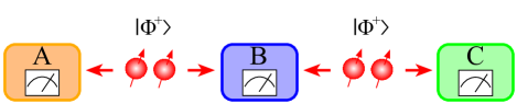
Figure 1: Experimental setup: independent sources each create entangled Bell states $|\Phi^{+}\rangle=(|00\rangle+|11\rangle)/\sqrt{2}$. From each state, one qubit is sent to Bob (B) who performs a measurement in the Bell state basis. One of the remaining qubits is sent to Alice (A), and the other is sent to Charlie (C). After Bob’s measurement, the residual entanglement is transferred to the qubit pair shared by Alice and Charlie. Alice performs a measurement of $x$, while Charlie performs a measurement of $z$.

Defining the joint conditional probability $P(abc|xz)$ as the probability that Alice obtains $a$, Bob obtains $b$, and Charlie obtains $c$ given a choice $xz$ for Alice’s and Charlie’s operators, a particularly interesting correlation function is Renou et al. (2021)

$$\Gamma=\sum_{abc,xz}w_{abc,xz}P(abc|xz),$$ (2)

where $w_{abc,xz}=\pm 1$ are weights Renou et al. (2021); Chen et al. (2022), $xz\in\left\{11,12,21,22,13,14,33,34,25,26,35,36\right\}$, and $abc\in\left\{0000,0001,\cdots,1110,1111\right\}$ so that the sum over $abc$ runs over the entire four-qubit computational basis. Specifically, one defines

$$\mathcal{T}_{b} = (-1)^{b_{2}}\left(S_{11}^{b}+S_{12}^{b}\right)+(-1)^{b_{1}}\left(S_{21}^{b}-S_{22}^{b}\right)$$ (3)

$$+ (-1)^{b_{2}}\left(S_{13}^{b}+S_{14}^{b}\right)-(-1)^{b_{1}+b_{2}}\left(S_{33}^{b}-S_{34}^{b}\right)$$

$$+ (-1)^{b_{1}}\left(S_{25}^{b}+S_{26}^{b}\right)-(-1)^{b_{1}+b_{2}}\left(S_{35}^{b}-S_{36}^{b}\right),$$

where

$$S_{xz}^{b}=\sum_{a,c=\pm 1}P(abc|xz),$$ (4)

and $b\in\left\{00,01,10,11\right\}$. The connection between $\Gamma$ and $\mathcal{T}_{b}$ is

$$\Gamma=\sum_{b}\mathcal{T}_{b}=6\sqrt{2}\approx 8.49,$$ (5)

where the approximate value represents an ideal score for a quantum description based on complex numbers.

It has been demonstrated Renou et al. (2021) that $\Gamma\lesssim 7.66$ for a standard formulation of quantum mechanics which relies upon only real quantities. The main goal of this work is to measure $\Gamma$ experimentally using IBM quantum devices. A quantum circuit which realizes this experiment is shown in Fig. 2. To make sense of the circuit, note that the two qubit basis states can be represented as two-component vectors

$$|0\rangle \dot{=}\left(\begin{array}[]{c}1\\ 0\end{array}\right),\;\;\;\;\;|1\rangle\dot{=}\left(\begin{array}[]{c}0\\ 1\end{array}\right).$$ (10)

The single-qubit Hadamard gate $\hat{H}$ acts according to $\hat{H}|0\rangle=\frac{1}{\sqrt{2}}\left(|0\rangle+|1\rangle\right)$, $\hat{H}|1\rangle=\frac{1}{\sqrt{2}}\left(|0\rangle-|1\rangle\right)$ and takes the matrix representation

$$\hat{H} \dot{=}\frac{1}{\sqrt{2}}\left(\begin{array}[]{cc}1&1\\ 1&-1\end{array}\right).$$ (13)

The controlled NOT (CNOT) gate flips a target qubit only if the control qubit is in the state $|1\rangle$, so its matrix representation is

CNOT $$\dot{=} \left(\begin{array}[]{cccc}1&0&0&0\\ 0&1&0&0\\ 0&0&0&1\\ 0&0&1&0\end{array}\right).$$ (18)

IBM hardware initializes all qubits in the quantum register to the $|0\rangle$ state. In order to create the entangled states $|\Phi^{+}\rangle$ required for the experiment, one may apply a combination of $\hat{H}$ and CNOT to the state $|00\rangle$ as depicted in Fig. 2 to obtain

$$\mbox{CNOT}_{i,j}[\hat{H}\otimes\hat{I}]|0\rangle_{i}\otimes|0\rangle_{j} = \frac{1}{\sqrt{2}}\left(|00\rangle+|11\rangle\right).$$ (19)

With two copies of $|\Phi^{+}\rangle$, Bob must perform a Bell state measurement (BSM) with one qubit from each pair. Measurement is only possible in the computational basis on IBM devices, so that any observer will only conclude that the qubit was in the state $|0\rangle$ or the state $|0\rangle$. However, it can be shown that the application of $\hat{H}$ followed by CNOT converts

$$|\Phi^{+}\rangle \rightarrow |00\rangle,$$

$$|\Phi^{-}\rangle \rightarrow |10\rangle,$$

$$|\Psi^{+}\rangle \rightarrow |01\rangle,$$

$$|\Psi^{-}\rangle \rightarrow |11\rangle.$$ (20)

Thus, Bob’s actual result of ‘00’, ‘01’, ‘10’, or ‘11’ allows an unambiguous determination of the two-qubit state in the Bell state basis prior to the gate transformations. For Alice and Charlie to measure Pauli operators $\hat{\sigma}^{j}$ (or combinations thereof), each must rotate the qubit to bring the measurement basis into the computational basis. Given an axis of rotation $P$, the rotation gate for angle $\theta$ is given by

$$\hat{R}_{\hat{\bf n}}(\theta)=\cos\frac{\theta}{2}\hat{I}-i\sin\frac{\theta}{2}\hat{\sigma}^{\hat{\bf n}}.$$ (21)

The basic idea is that one can measure $\hat{\sigma}^{\hat{\bf n}}$ where $\hat{\bf n}=\cos\phi\sin\theta\hat{\bf x}+\sin\phi\sin\theta\hat{\bf y}+\cos\theta\hat{\bf z}$ by first rotating the qubit by $-\phi$ about the $z$-axis (applying $R_{z}(-\phi)$ and then rotating by $-\theta$ about the $y$-axis (applying $R_{y}(-\theta)$ to bring the relevant measurement into the computational basis. Given Alice’s choice of $x\in\left\{\hat{\sigma}^{z},\hat{\sigma}^{x},\hat{\sigma}^{y}\right\}$ and Charlie’s choice $z\in\left\{(\hat{\sigma}^{z}\pm\hat{\sigma}^{x})/\sqrt{2},(\hat{\sigma}^{z}\pm\hat{\sigma}^{y})/\sqrt{2},(\hat{\sigma}^{x}\pm\hat{\sigma}^{y})/\sqrt{2}\right\}$, there are a total of $18$ individual configurations $xz$. Of these, 12 are used in the computation of $\Gamma$, so we restrict attention to $xz\in\left\{11,12,21,22,13,14,33,34,25,26,35,36\right\}$. For example, $xz=36$ corresponds to Alice measuring $\hat{\sigma}^{y}$ and Charlie measuring $(\hat{\sigma}^{x}-\hat{\sigma}^{y})/\sqrt{2}$. To rotate each qubit appropriately so that a computational-basis measurement returns each of these spin projections, Alice must rotate her qubit by $-\phi_{1}=-\frac{\pi}{2}$ about the $z$-axis followed by a rotation of $-\theta_{1}=-\frac{\pi}{2}$ (with $\phi_{1}=0$) about the $y$ axis. Charlie must rotate his qubit by $-\phi_{2}=\frac{\pi}{4}$ about the $z$-axis and then by $-\theta_{2}=-\frac{\pi}{2}$ about the $y$-axis. A complete list of rotation angles $\phi_{1,2}$, $\theta_{1,2}$ for each choice of $xz$ is given below in Table 1

$xz$	$\phi_{1}$	$\theta_{1}$	$\phi_{2}$	$\theta_{2}$
11	0	0	0	$\pi/4$
12	0	0	0	$-\pi/4$
21	0	$\pi/2$	0	$\pi/4$
22	0	$\pi/2$	0	$-\pi/4$
13	0	0	$\pi/2$	$\pi/4$
14	0	0	$-\pi/2$	$\pi/4$
33	$\pi/2$	$\pi/2$	$\pi/2$	$\pi/4$
34	$\pi/2$	$\pi/2$	$-\pi/2$	$\pi/4$
25	0	$\pi/2$	$\pi/4$	$\pi/2$
26	0	$\pi/2$	$-\pi/4$	$\pi/2$
35	$\pi/2$	$\pi/2$	$\pi/4$	$\pi/2$
36	$\pi/2$	$\pi/2$	$-\pi/4$	$\pi/2$

Table 1: Rotation angles used for all 12 cases of $xz$.

Figure 2: Circuit to run on IBM Quantum devices: two pairs of Bell states $|\Phi^{+}\rangle$ are created. Bob performs a Bell state measurement on a pair constructed from both sets of qubits, while Alice and Charlie make particular measurements on the two remaining qubits.

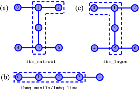
Figure 3: Qubit connectivity and actual usage in this work for IBM devices used: (a) qubits 2,1,3,5 were used on ibm_nairobi; (b) qubits 0,1,2,3 were used on ibmq_manila and ibmq_lima; (c) qubits 0,1,3,5 were used on ibm_lagos.

The circuit in Fig. 2 can be used to reconstruct the joint conditional probability distribution $P(abc|xz)$ needed to evaluate the score $\Gamma$ in Eq. (2) by randomly choosing measurements $xz$ and repeatedly executing the circuit. It is possible to sample $xz$ randomly and send a set of circuits to the IBM devices for single-shot experiments. However, one is limited by the maximum number of circuits which can be executed within a particular job, so the maximum number of single-shot runs is $\mathcal{O}(10^{2})$. Since one may execute the same circuit for at least 20,000 “shots,” it is computationally advantageous to execute each of the 12 possible cases of $xz$ for some equal and large number of shots. In what follows, the random sampling over $xz$ will be mimicked by an equal sampling of $N\geq 20,000$ shots over each of the 12 configurations for $xz$.

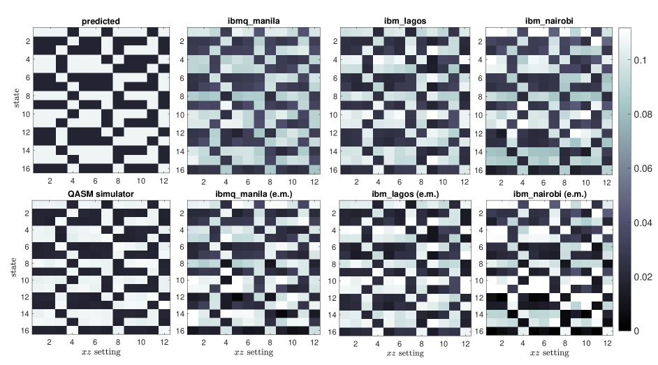
Figure 4: Final circuit results, $P(abc|xz)$, where the 16 possible four-qubit states are indexed vertically and the horizontal axis depicts one of the 12 possible Alice/Charlie measurement combinations $xz$. Theoretical prediction (upper left) follows from standard quantum mechanics calculation of the gate operations; QASM simulator refers to IBM’s quantum assembly language (QASM) simulator. The label “e.m.” on lower plots indicates that basic readout error mitigation as described in the text has been performed.

To minimize errors in the execution of the circuit in Fig. 2, it is essential to ensure the physical qubits employed are connected in such a way that the CNOT gates can be implemented directly. The currently available IBM Quantum devices possess several types of qubit topology. Figure 3 depicts which subset of qubits is chosen for each device used. While multiple options are typically available for each device, the particular choices used in this work are dictated by trying to minimize CNOT and measurement readout errors. Detailed calibration information is included in the supplemental material sup .

III Results

The circuit in Fig. 2 has been sent to several IBM Quantum devices: ibmq_lima v1.0.35, a Falcon r4T processor; ibmq_manila v1.0.29, a Falcon r5.11L processor; ibm_lagos v1.0.27, a Falcon r5.11H processor; and ibm_nairobi v1.0.26, a Falcon 5.11H processor. The first two machines are five-qubit devices which are freely available, while ibm_lagos is a seven-qubit device currently available to members of the IBM Quantum Researchers Program IBM (b). The device ibm_nairobi is a freely-available, seven-qubit processor. For the five-qubit devices, 20,000 executions (“shots”) per choice of $xz$ are employed in a single job. The seven qubit devices allowed 32,000 shots per choice of $xz$. Each job yielded a list of counts for each of the 16 possible four-qubit states. The conditional probabilities $P(abc|xz)$ can then be reconstructed, and $\Gamma$ can be computed from Eq. (2). Samples of reconstructed probability distributions using several devices are shown in Fig. 4 along with results from the Quantum Assembly Language (QASM) simulator and theoretical predictions. The QASM simulator is used to verify that the circuit accurately simulates the experiment in an ideal, noise-free environment with only statistical fluctuations.

With $\mathcal{O}(10^{4})$ shots per choice of $xz$, statistical fluctuations are expected to be small. Noise in the devices leads to errors which can be orders of magnitude larger than statistical fluctuations. Additionally, the devices are calibrated daily, leading to more significant variations in results from day to day than predicted from statistical analysis (e.g., standard error of mean). We quantify the uncertainty associated with all of these factors roughly by repeating the job at least three times per experiment for three separate experiments. For example, we performed measurements using ibm_lagos on the following dates: 2022-04-12, 2022-04-19, 2022-04-24. From each measurement date, we store the lowest, highest, and median score obtained for the $n\geq$ measurements of $\Gamma$. The nine points consisting of these three values from three temporally-separated experiments are used to compute the values (mean $\Gamma$ and standard deviation $\sigma$) summarized in Table 2 and depicted graphically in Fig. 5. All data collected, as well as relevant calibration metrics obtained during the measurement events, are tabulated in the supplemental material sup .

Device	Shots per $xz$	$\;\Gamma$	$\sigma$
QASM simulator	32,000	8.486	0.015
ibmq_lima	20,000	7.680	0.041
ibmq_manila	20,000	7.823	0.151
ibm_lagos	32,000	8.046	0.065
ibm_nairobi	32,000	8.410	0.072

Table 2: Measured (mean) scores and standard deviation for the QASM simulator and IBM devices employing basic readout error mitigation averaged over data collected across several days during which multiple device calibrations occur between computations.

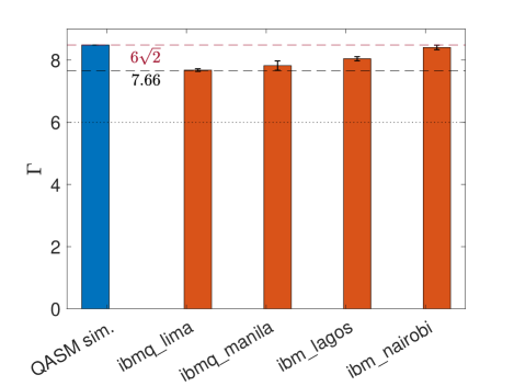
Figure 5: Mean score $\Gamma$ for the QASM simulator and various IBM devices across several days (see main text) with readout error mitigation applied to results for actual devices. The lower dotted line denotes the quantum/classical boundary $\Gamma=6$, the lower dashed line at $\Gamma\approx 7.66$ denotes the upper limit for real variables, and the upper dashed line $\Gamma=6\sqrt{2}$ denotes the ideal score for a complex quantum system. Error bars correspond to $\sigma$ described in main text.

Results in Table 2 detail measured values of $\Gamma$ after applying basic, readout-error mitigation Abbas et al. (2020). To motivate the readout error mitigation, note that any job returns a set of “counts” as its result. As a simplified example, consider a two-qubit system in which both qubits are measured. The final result will be a set of counts corresponding to the number of times each of the four possible two-qubit states is measured. In the simplest possible two-qubit circuit, one creates a state (say $|00\rangle$) and measures both qubits. Supposing this circuit is run $N=1024$ times, the existence of errors means that measurements will not always correspond to the state $|00\rangle$. As an example, one might find $900$ instances of $|00\rangle$, $61$ instances of $|01\rangle$, $54$ instances of $|10\rangle$, and $9$ instances of $|11\rangle$. Repeating this process for all two-qubit states $|b_{0}b_{1}\rangle$ with $b_{0,1}\in\left\{0,1\right\}$, one may build a calibration matrix ${\bf C}$ for which each of these calibration runs yields a row,

$${\bf m}_{\mbox{\scriptsize exp}}={\bf C}{\bf m}_{\mbox{\scriptsize ideal}}.$$ (22)

Here ${\bf m}_{\mbox{\scriptsize exp}}$ are the obtained counts (in the basis $|00\rangle,\cdots,|11\rangle$, and ${\bf m}_{\mbox{\scriptsize ideal}}$ are the expected results. This matrix ${\bf C}$ obtained from basic state measurement on a particular device can then be inverted and interpreted as an average correction transformation for results obtained for any circuit which should approximately correct for any measurement errors in the readout process. In this work, we only consider this most basic type of error mitigation.

One potentially problematic aspect of this simple procedure is that the corrected counts can attain negative values, which is clearly unphysical. It is still possible to compute reasonable expectation values from these corrected counts, interpreting the potentially negative probabilities as quasiprobabilities. In our application of this procedure, negative counts are obtained as corrected counts for some results obtained on ibmq_lima, ibmq_nairobi, and for a small number ($n=3$) of individual results from ibmq_manila. No results obtained from ibmq_lagos yielded negative counts upon applying the basic readout-error mitigation described above, and the magnitudes of the negative counts from other devices are fairly small fractions ($\lesssim 10^{-2}$) of the total shots per job. Regardless, it is desirable to explore whether such negative counts can artificially inflate the overall score $\Gamma$ in a given experiment. An alternative procedure to the direct inversion of ${\bf C}$ is to perform a constrained least-squares optimization to solve the system

$${\bf y} = {\bf A}{\bf x}$$ (23)

for ${\bf x}={\bf m}_{\mbox{\scriptsize ideal}}$, given ${\bf A}={\bf C}$ and ${\bf y}={\bf m}_{\mbox{\scriptsize exp}}$. The constraint $x_{i}>0$ is applied to yield a non-negative probability distribution ${\bf x}$, where normalization is imposed so that $||{\bf x}||_{2}=1$. The procedure can be implemented easily using the SciPy Virtanen et al. (2020) optimization routine nnls(A,y) or the Matlab MATLAB (2022) function lsqnonneg(A,y), both based on the algorithm published by Lawson and Hanson Lawson and Hanson (1987). Results obtained with constrained optimization are identical to those obtained by directly inverting the calibration matrix when negative counts are not obtained. While the effective difference in computation of $\Gamma$ is fairly small, the reported values for $\Gamma$ in Table 2 correspond the the smaller score obtained from constrained optimization where any difference occurs. All scores obtained using both types of readout-error mitigation are included in the supplemental material sup . Where any difference occurs, the constrained optimization yields a (slightly) lower score. It should be noted that the particular form of readout-error mitigation—basic inversion of the measurable calibration matrix and least-squares optimization—is not necessarily scalable to large systems Nation et al. (2021). However, these basic methods are easily applied to the simple circuit considered in this work.

From Table 2 and Fig. 5, it is evident that the noisiest device, ibmq_lima, yielded values of $\Gamma$ which hover around the boundary between real-valued and complex-valued quantum mechanics Renou et al. (2021). The devices ibmq_manila, ibm_lagos, and ibm_nairobi give values for $\Gamma$ which comfortably exceed this bound of 7.66, but only the seven qubit devices give results for $\Gamma$ which decisively exceed $\Gamma_{\mbox{\scriptsize crit}}$ when fluctuations across several days are taken into account with the estimate of standard deviation $\sigma$.

A potentially confounding aspect of using cloud-based devices to perform experiments via Qiskit is that the user has little control over the calibration and tuning of the devices. Strictly speaking, the Qiskit Pulse programming kit Qis (b) does afford users the ability to specify pulse-level timing dynamics in the hardware. Such low-level control could potentially improve the quality of results obtained from these devices. The intent of the present work is to demonstrate that certain devices (e.g., ibm_lagos, ibm_nairobi ) can deliver reliable results for Bell-test-like experiments even without such low-level control. Only a basic working knowledge of quantum circuits with the simplest form of readout-error mitigation is necessary to obtain the results presented.

IBM devices are calibrated daily, and the relevant parameters are easily accessible to users. The calibrations affect the tuning of microwave pulses used to manipulate the qubits, and these daily calibrations tend to cause the results to “drift” significantly compared to differences attributable to statistical fluctuations for results collected within the same day. Data have been collected across several days during which several calibrations cycles have occurred. Detailed calibration information is collected in the supplemental material sup . The data collected from ibm_lagos and ibm_nairobi give results which are consistently well above the real/complex threshold. The results from ibmq_lima and ibmq_manila drift substantially enough that making firm conclusions from these results is difficult.

An interesting question concerns how consistently these results can be obtained over longer time scales. That is, this technology would not be particularly useful for performing experiments if the results varied substantially over a period of weeks or months. The data collection described in Sec. II took place over a period of 10-14 days to allow several system calibrations to occur between individual experiments. While the score fluctuations within a particular day appeared well described by the same statistical uncertainty associated with the QASM simulator results, significantly larger drift in the score was observed across different days. Presumably such drift follows from device calibration which resulted in new values for readout error rates and other system parameters. A detailed table of system parameters for each device used during each period of data collection can be found in the supplemental material sup . However, collecting data in three sets over a period of 14 days does little to address the consistency of results over significant timescales. Indeed, it is much less impressive to obtain a score $\Gamma>\Gamma_{\mbox{\scriptsize crit}}$ if it is not reproducible on the same device several weeks later.

To address how robust the results are over longer timescales, we have repeated the experiment using the same qubits on ibm_lagos roughly six months after initial data collection. While ibm_nairobi gives consistently stronger results, it was not available on the IBM cloud during the initial phase of data collection. Upon repeating the data collection in October 2022, we obtain $\Gamma=8.115\pm 0.042$ compared to $\Gamma=8.046\pm 0.065$ as obtained in April 2022.

IV Discussion

Given that the results from ibm_lagos and ibm_nairobi are robust with respect to daily calibrations in yielding an experimental score of $\Gamma\geq 8.0>7.66$, it is notable that Ref. Chen et al., 2022 found $\Gamma=8.09(1)$ using a custom-designed quantum processor. The IBM devices ibm_lagos and ibm_nairobi yield scores $\Gamma=8.046\pm 0.065$ and $\Gamma=8.410\pm 0.074$, respectively. Thus, the present work shows that the freely-available IBM processors are capable of obtaining convincing results for the necessity of complex numbers in the traditional formulation of quantum mechanics while only requiring the user to arrange a set of basic quantum circuit elements. No device yields impressive results without readout-error mitigation, but all hardware considered yields experimental values of $\Gamma$ which approach or exceed the threshold for the necessity of complex numbers in a traditional formulation of quantum mechanics.

Drift in results due to the daily calibration of IBM devices makes definitive results difficult to extract from the five-qubit devices in this particular experiment, but the results from ibm_lagos and ibm_nairobi appear to not experience substantial drift and are in good agreement with previous experimental results Chen et al. (2022); Li et al. (2022); Wu et al. (2022). Taken together, the results confirm the fairly primitive nature of currently available hardware while also demonstrating that some hardware is capable of performing delicate experiments consistently. Moreover, we have demonstrated that the results of at least one device (ibm_lagos) are consistent over a timescale of about several months, despite the numerous daily calibrations.

In addition to the scientific value of performing experiments which probe foundational features of quantum mechanics on freely-available quantum hardware, there is another opportunity afforded by the use of these Bell tests: benchmarking particular quantum devices. With careful experiments being performed that can conclusively determine the expected outcome for such Bell tests Chen et al. (2022); Li et al. (2022); Wu et al. (2022), these types of tests can be seen as a particular way to benchmark the performance of quantum hardware Sheffer et al. (2022); Wang et al. (2021); Sadana et al. (2022); Santini and Vitale (2022). Quantifying the degree to which these devices accurately simulate quantum processes is difficult. Even with the detailed calibration information readily accessible sup , it is not clear how to predict how well a given device will perform on any particular task. In the data collected for this work, there was no clear correlation between particular calibration metrics (e.g., average or maximum $CNOT$ error rate) and the final score obtained. It would be an interesting direction for future work to perform a careful multivariable regression or make use of techniques from machine learning to explore whether certain combinations of calibration metrics directly correlate with higher scores.

Supplementary Material

IV.1 Calibration data

Tables S1–S8 depict calibration metrics for the devices used at the time these devices were used to generate the data depicted in the main text. As the IBM devices are calibrated on an approximately daily basis, the actual results obtained from the hardware can drift substantially from day to day. Calibration metrics affect the precise manner in which circuit gates implemented in Qiskit are translated into microwave pulses used to manipulate the physical qubits. Each quantum circuit used in this work has been executed at least 20,000 times, resulting in a fairly small statistical uncertainty which is generally smaller than the “drift” in results that occurs as a consequence of daily calibrations.

IV.1.1 ibmq_lima

Date	qubit	$T_{1}$ ($\mu$s)	$T_{2}$ ($\mu$s)	freq. (GHz)	Anharmonicity (GHz)	readout assignment error
2022-04-14	0	93.46	118.47	5.030	$-0.33574$	$1.78\times 10^{-2}$
2022-04-14	1	122.62	131.38	5.128	$-0.31835$	$1.67\times 10^{-2}$
2022-04-14	2	117.13	131.29	5.247	$-0.33360$	$2.22\times 10^{-2}$
2022-04-14	3	135.20	106.71	5.303	$-0.33124$	$2.68\times 10^{-2}$
2022-04-14	4	21.41	21.57	5.092	$-0.33447$	$5.10\times 10^{-2}$
2022-04-19	0	71.55	97.69	5.030	$-0.33574$	$2.27\times 10^{-2}$
2022-04-19	1	123.87	107.28	5.128	$-0.31835$	$1.50\times 10^{-2}$
2022-04-19	2	123.98	134.58	5.247	$-0.33360$	$2.30\times 10^{-2}$
2022-04-19	3	96.41	96.81	5.303	$-0.33124$	$2.92\times 10^{-2}$
2022-04-19	4	22.11	22.55	5.092	$-0.33447$	$6.20\times 10^{-2}$
2022-04-24	0	169.65	188.84	5.030	$-0.33574$	$2.30\times 10^{-2}$
2022-04-24	1	125.59	117.96	5.128	$-0.31835$	$1.47\times 10^{-2}$
2022-04-24	2	78.30	96.82	5.247	$-0.33360$	$2.22\times 10^{-2}$
2022-04-24	3	101.35	69.09	5.303	$-0.33124$	$3.31\times 10^{-2}$
2022-04-24	4	23.48	22.98	5.092	$-0.33447$	$4.82\times 10^{-2}$

Table S1: Calibration data for qubits in ibmq_lima.

Date	connection	error rate	gate time (ns)
2022-04-14	0-1	$5.290\times 10^{-3}$	305.777
2022-04-14	1-2	$2.632\times 10^{-2}$	334.222
2022-04-14	1-3	$1.263\times 10^{-2}$	497.777
2022-04-14	3-4	$1.680\times 10^{-2}$	519.111
2022-04-19	0-1	$5.247\times 10^{-3}$	305.777
2022-04-19	1-2	$7.718\times 10^{-2}$	334.222
2022-04-19	1-3	$1.171\times 10^{-2}$	497.778
2022-04-19	3-4	$1.707\times 10^{-2}$	519.111
2022-04-24	0-1	$4.707\times 10^{-3}$	305.777
2022-04-24	1-2	$7.186\times 10^{-2}$	334.222
2022-04-24	1-3	$1.184\times 10^{-2}$	497.777
2022-04-24	3-4	$1.905\times 10^{-2}$	519.111

Table S2: Calibration data for CNOT gates in ibmq_lima.

IV.1.2 ibmq_manila

Date	qubit	$T_{1}$ ($\mu$s)	$T_{2}$ ($\mu$s)	freq. (GHz)	Anharmonicity (GHz)	readout assignment error
2022-04-15	0	107.80	66.96	4.962	$-0.34335$	$2.70\times 10^{-2}$
2022-04-15	1	135.11	74.09	4.838	$-0.34621$	$6.37\times 10^{-2}$
2022-04-15	2	157.35	22.65	5.037	$-0.34366$	$4.16\times 10^{-2}$
2022-04-15	3	197.38	65.29	4.951	$-0.34355$	$2.50\times 10^{-2}$
2022-04-15	4	138.50	45.29	5.065	$-0.34211$	$2.97\times 10^{-2}$
2022-04-16	0	118.95	81.42	4.962	$-0.34335$	$3.0\times 10^{-2}$
2022-04-16	1	124.02	65.34	4.838	$-0.34621$	$3.41\times 10^{-2}$
2022-04-16	2	165.67	25.97	5.037	$-0.34366$	$3.37\times 10^{-2}$
2022-04-16	3	179.13	52.80	4.951	$-0.34355$	$2.24\times 10^{-2}$
2022-04-16	4	178.07	49.40	5.065	$-0.34211$	$3.72\times 10^{-2}$
2022-04-18	0	104.63	69.26	4.962	$-0.34335$	$2.91\times 10^{-2}$
2022-04-18	1	170.83	53.51	4.838	$-0.34621$	$4.80\times 10^{-2}$
2022-04-18	2	207.92	25.92	5.037	$-0.34366$	$2.79\times 10^{-2}$
2022-04-18	3	147.05	53.80	4.951	$-0.34355$	$2.17\times 10^{-2}$
2022-04-18	4	156.62	43.58	5.065	$-0.34211$	$3.07\times 10^{-2}$
2022-04-19	0	131.94	70.25	4.962	$-0.34335$	$3.38\times 10^{-2}$
2022-04-19	1	130.10	76.29	4.838	$-0.34621$	$2.92\times 10^{-2}$
2022-04-19	2	142.48	25.95	5.037	$-0.34366$	$2.44\times 10^{-2}$
2022-04-19	3	157.93	60.11	4.951	$-0.34355$	$1.90\times 10^{-2}$
2022-04-19	4	170.45	41.78	5.065	$-0.34211$	$2.59\times 10^{-2}$
2022-04-24	0	199.20	99.76	4.962	$-0.34335$	$3.2\times 10^{-2}$
2022-04-24	1	195.62	72.03	4.838	$-0.34621$	$3.18\times 10^{-2}$
2022-04-24	2	158.43	24.61	5.037	$-0.34366$	$4.64\times 10^{-2}$
2022-04-24	3	159.02	40.88	4.951	$-0.34355$	$3.23\times 10^{-2}$
2022-04-24	4	130.71	40.62	5.065	$-0.34211$	$2.29\times 10^{-2}$
2022-04-26	0	157.59	104.06	4.962	$-0.34335$	$3.55\times 10^{-2}$
2022-04-26	1	226.17	77.01	4.838	$-0.34621$	$2.82\times 10^{-2}$
2022-04-26	2	188.27	25.22	5.037	$-0.34366$	$2.66\times 10^{-2}$
2022-04-26	3	228.95	64.21	4.951	$-0.34355$	$2.28\times 10^{-2}$
2022-04-26	4	124.87	45.25	5.065	$-0.34211$	$2.97\times 10^{-2}$

Table S3: Calibration data for qubits in ibmq_manila.

Date	connection	error rate	gate time (ns)
2022-04-15	0-1	$8.959\times 10^{-3}$	277.333
2022-04-15	1-2	$1.114\times 10^{-2}$	469.333
2022-04-15	2-3	$7.623\times 10^{-3}$	355.556
2022-04-15	3-4	$5.750\times 10^{-3}$	334.222
2022-04-16	0-1	$6.807\times 10^{-3}$	277.333
2022-04-16	1-2	$1.049\times 10^{-2}$	469.333
2022-04-16	2-3	$6.371\times 10^{-3}$	355.556
2022-04-16	3-4	$5.498\times 10^{-3}$	334.222
2022-04-18	0-1	$9.176\times 10^{-3}$	277.333
2022-04-18	1-2	$1.180\times 10^{-2}$	469.333
2022-04-18	2-3	$7.778\times 10^{-3}$	355.556
2022-04-18	3-4	$6.451\times 10^{-3}$	334.222
2022-04-19	0-1	$7.651\times 10^{-3}$	277.333
2022-04-19	1-2	$9.658\times 10^{-3}$	469.333
2022-04-19	2-3	$6.794\times 10^{-3}$	355.556
2022-04-19	3-4	$6.265\times 10^{-3}$	334.222
2022-04-24	0-1	$5.223\times 10^{-3}$	277.333
2022-04-24	1-2	$9.977\times 10^{-3}$	469.333
2022-04-24	2-3	$9.831\times 10^{-3}$	355.556
2022-04-24	3-4	$6.666\times 10^{-3}$	334.222
2022-04-26	0-1	$6.681\times 10^{-3}$	277.333
2022-04-26	1-2	$1.550\times 10^{-2}$	469.333
2022-04-26	2-3	$6.702\times 10^{-3}$	355.556
2022-04-26	3-4	$5.201\times 10^{-3}$	334.222

Table S4: Calibration data for CNOT gates in ibmq_manila.

IV.1.3 ibm_lagos

Date	qubit	$T_{1}$ ($\mu$s)	$T_{2}$ ($\mu$s)	freq. (GHz)	Anharmonicity (GHz)	readout assignment error
2022-04-12	0	110.77	46.41	5.235	$-0.33987$	$7.30\times 10^{-3}$
2022-04-12	1	130.34	84.81	5.100	$-0.34325$	$1.14\times 10^{-2}$
2022-04-12	2	123.18	112.70	5.188	$-0.34193$	$5.40\times 10^{-3}$
2022-04-12	3	207.35	143.35	4.987	$-0.34529$	$1.97\times 10^{-2}$
2022-04-12	4	161.92	46.82	5.285	$-0.33923$	$1.20\times 10^{-2}$
2022-04-12	5	133.28	88.03	5.176	$-0.34079$	$1.18\times 10^{-2}$
2022-04-12	6	137.78	178.13	5.064	$-0.34276$	$5.30\times 10^{-3}$
2022-04-19	0	131.57	49.25	5.235	$-0.33987$	$7.60\times 10^{-3}$
2022-04-19	1	138.38	116.49	5.100	$-0.34325$	$1.11\times 10^{-2}$
2022-04-19	2	112.36	142.46	5.188	$-0.34193$	$4.90\times 10^{-3}$
2022-04-19	3	105.22	93.65	4.987	$-0.34529$	$1.99\times 10^{-2}$
2022-04-19	4	107.02	43.79	5.285	$-0.33923$	$1.37\times 10^{-2}$
2022-04-19	5	129.64	83.89	5.176	$-0.34079$	$1.28\times 10^{-2}$
2022-04-19	6	180.21	109.66	5.064	$-0.34276$	$7.50\times 10^{-3}$
2022-04-24	0	187.41	49.35	5.235	$-0.33987$	$8.70\times 10^{-3}$
2022-04-24	1	117.38	118.40	5.100	$-0.34325$	$8.90\times 10^{-3}$
2022-04-24	2	64.03	119.95	5.188	$-0.34193$	$6.80\times 10^{-3}$
2022-04-24	3	145.37	140.26	4.987	$-0.34529$	$1.66\times 10^{-2}$
2022-04-24	4	167.96	51.35	5.285	$-0.33923$	$1.41\times 10^{-2}$
2022-04-24	5	91.06	77.16	5.176	$-0.34079$	$1.18\times 10^{-2}$
2022-04-24	6	127.67	146.32	5.064	$-0.34276$	$7.60\times 10^{-3}$
2022-09-28	0	122.09	43.23	5.235	$-0.33987$	$7.70\times 10^{-3}$
2022-09-28	1	122.50	79.85	5.100	$-0.34325$	$8.70\times 10^{-3}$
2022-09-28	2	80.70	143.44	5.188	$-0.34193$	$4.00\times 10^{-3}$
2022-09-28	3	179.06	96.01	4.987	$-0.34529$	$1.60\times 10^{-2}$
2022-09-28	4	70.89	19.19	5.285	$-0.33923$	$1.27\times 10^{-2}$
2022-09-28	5	125.56	80.26	5.176	$-0.34079$	$1.26\times 10^{-2}$
2022-09-28	6	135.57	108.60	5.064	$-0.34276$	$8.90\times 10^{-3}$
2022-10-02	0	122.09	49.23	5.235	$-0.33987$	$7.70\times 10^{-3}$
2022-10-02	1	122.5	79.85	5.100	$-0.34325$	$8.70\times 10^{-3}$
2022-10-02	2	80.70	143.33	5.188	$-0.34193$	$4.00\times 10^{-3}$
2022-10-02	3	179.06	96.01	4.987	$-0.34529$	$1.60\times 10^{-2}$
2022-10-02	4	70.89	19.19	5.285	$-0.33923$	$1.27\times 10^{-2}$
2022-10-02	5	125.55	80.26	5.176	$-0.34079$	$1.26\times 10^{-2}$
2022-10-02	6	135.57	108.60	5.064	$-0.34276$	$8.90\times 10^{-3}$
2022-10-08	0	84.09	30.77	5.235	$-0.33987$	$8.10\times 10^{-3}$
2022-10-08	1	128.29	106.63	5.100	$-0.34325$	$9.80\times 10^{-3}$
2022-10-08	2	163.44	149.43	5.188	$-0.34193$	$6.70\times 10^{-3}$
2022-10-08	3	141.19	88.05	4.987	$-0.34529$	$2.00\times 10^{-2}$
2022-10-08	4	14.20	14.23	5.285	$-0.33923$	$1.38\times 10^{-2}$
2022-10-08	5	119.10	89.16	5.176	$-0.34079$	$1.25\times 10^{-2}$
2022-10-08	6	131.13	133.12	5.064	$-0.34276$	$7.40\times 10^{-3}$

Table S5: Calibration data for qubits in ibm_lagos.

Date	connection	error rate	gate time (ns)
2022-04-12	0-1	$6.544\times 10^{-3}$	305.777
2022-04-12	1-2	$6.707\times 10^{-3}$	327.111
2022-04-12	1-3	$9.804\times 10^{-3}$	334.222
2022-04-12	3-5	$1.061\times 10^{-2}$	334.222
2022-04-12	4-5	$5.090\times 10^{-3}$	362.667
2022-04-12	5-6	$3.599\times 10^{-3}$	256.000
2022-04-19	0-1	$7.808\times 10^{-3}$	305.777
2022-04-19	1-2	$5.743\times 10^{-3}$	327.111
2022-04-19	1-3	$8.710\times 10^{-3}$	334.222
2022-04-19	3-5	$1.513\times 10^{-2}$	334.222
2022-04-19	4-5	$5.895\times 10^{-3}$	362.667
2022-04-19	5-6	$4.501\times 10^{-3}$	256.000
2022-04-24	0-1	$7.570\times 10^{-3}$	305.777
2022-04-24	1-2	$5.387\times 10^{-3}$	327.111
2022-04-24	1-3	$5.706\times 10^{-3}$	334.222
2022-04-24	3-5	$8.753\times 10^{-3}$	334.222
2022-04-24	4-5	$4.983\times 10^{-3}$	362.667
2022-04-24	5-6	$5.735\times 10^{-3}$	256.000
2022-09-28	0-1	$6.213\times 10^{-3}$	305.777
2022-09-28	1-2	$5.485\times 10^{-3}$	327.111
2022-09-28	1-3	$5.011\times 10^{-3}$	334.222
2022-09-28	3-5	$9.463\times 10^{-3}$	334.222
2022-09-28	4-5	$8.606\times 10^{-3}$	362.667
2022-09-28	5-6	$6.566\times 10^{-3}$	256.000
2022-10-02	0-1	$6.860\times 10^{-3}$	305.777
2022-10-02	1-2	$5.756\times 10^{-3}$	327.111
2022-10-02	1-3	$6.382\times 10^{-3}$	334.222
2022-10-02	3-5	$1.243\times 10^{-2}$	334.222
2022-10-02	4-5	$1.116\times 10^{-2}$	362.667
2022-10-02	5-6	$6.629\times 10^{-3}$	256.000
2022-10-08	0-1	$6.613\times 10^{-3}$	305.777
2022-10-08	1-2	$4.230\times 10^{-3}$	327.111
2022-10-08	1-3	$6.692\times 10^{-3}$	334.222
2022-10-08	3-5	$9.568\times 10^{-3}$	334.222
2022-10-08	4-5	$7.202\times 10^{-3}$	362.667
2022-10-08	5-6	$5.620\times 10^{-3}$	256.000

Table S6: Calibration data for CNOT gates in ibm_lagos.

IV.1.4 ibm_nairobi

Date	qubit	$T_{1}$ ($\mu$s)	$T_{2}$ ($\mu$s)	freq. (GHz)	Anharmonicity (GHz)	readout assignment error
2022-09-28	0	160.60	36.77	5.260	$-0.33983$	$2.41\times 10^{-2}$
2022-09-28	1	159.05	84.96	5.170	$-0.34058$	$3.74\times 10^{-2}$
2022-09-28	2	106.63	81.60	5.274	$-0.33890$	$2.47\times 10^{-2}$
2022-09-28	3	162.92	33.89	5.027	$-0.34253$	$3.41\times 10^{-2}$
2022-09-28	4	92.94	69.85	5.177	$-0.34059$	$1.92\times 10^{-2}$
2022-09-28	5	156.20	19.75	5.293	$-0.34053$	$2.61\times 10^{-2}$
2022-09-28	6	130.98	60.91	5.129	$-0.34044$	$1.55\times 10^{-1}$
2022-10-01	0	142.69	35.23	5.260	$-0.33983$	$2.20\times 10^{-2}$
2022-10-01	1	135.93	101.47	5.170	$-0.34058$	$3.14\times 10^{-2}$
2022-10-01	2	92.71	101.33	5.274	$-0.33890$	$2.29\times 10^{-2}$
2022-10-01	3	150.06	71.35	5.027	$-0.34253$	$3.18\times 10^{-2}$
2022-10-01	4	126.71	74.76	5.177	$-0.34059$	$1.76\times 10^{-2}$
2022-10-01	5	152.14	20.97	5.293	$-0.34053$	$3.22\times 10^{-2}$
2022-10-01	6	165.52	106.79	5.129	$-0.34044$	$2.85\times 10^{-2}$
2022-10-07	0	151.12	30.06	5.260	$-0.33983$	$2.75\times 10^{-2}$
2022-10-07	1	112.45	94.07	5.170	$-0.34058$	$2.53\times 10^{-2}$
2022-10-07	2	132.64	205.77	5.274	$-0.33890$	$2.32\times 10^{-2}$
2022-10-07	3	166.22	69.41	5.027	$-0.34253$	$3.94\times 10^{-2}$
2022-10-07	4	77.26	75.22	5.177	$-0.34059$	$1.97\times 10^{-2}$
2022-10-07	5	121.90	21.08	5.293	$-0.34053$	$2.82\times 10^{-2}$
2022-10-07	6	152.98	96.51	5.129	$-0.34044$	$2.48\times 10^{-2}$

Table S7: Calibration data for qubits in ibm_nairobi.

Date	connection	error rate	gate time (ns)
2022-09-28	0-1	$1.040\times 10^{-2}$	248.889
2022-09-28	1-2	$1.668\times 10^{-2}$	426.667
2022-09-28	1-3	$1.233\times 10^{-2}$	270.222
2022-09-28	3-5	$1.792\times 10^{-2}$	277.333
2022-09-28	4-5	$5.119\times 10^{-3}$	312.889
2022-09-28	5-6	$7.943\times 10^{-3}$	341.333
2022-10-01	0-1	$1.153\times 10^{-2}$	248.889
2022-10-01	1-2	$8.893\times 10^{-3}$	426.667
2022-10-01	1-3	$9.813\times 10^{-3}$	270.222
2022-10-01	3-5	$1.338\times 10^{-2}$	277.333
2022-10-01	4-5	$4.588\times 10^{-3}$	312.889
2022-10-01	5-6	$9.002\times 10^{-3}$	341.333
2022-10-07	0-1	$9.965\times 10^{-3}$	248.889
2022-10-07	1-2	$7.843\times 10^{-3}$	426.667
2022-10-07	1-3	$8.187\times 10^{-3}$	270.222
2022-10-07	3-5	$1.258\times 10^{-2}$	277.333
2022-10-07	4-5	$6.003\times 10^{-3}$	312.889
2022-10-07	5-6	$5.854\times 10^{-3}$	341.333

Table S8: Calibration data for CNOT gates in ibm_nairobi.

IV.2 Individual scores

As noted in the main text, several experimental runs were performed during each period of data collection, resulting in at least three scores. Due to device constraints or queue times, it was possible to obtain more than three data points for certain devices on certain devices. In the event more than three points were obtained, the lowest, largest, and median score were used from the particular run for figures and results presented in the main text. Below we collect the raw (uncorrected) scores, the scores in which basic error mitigation was performed via inversion of the calibration matrix, and error-mitigated scores resulting from a constrained optimization approach. If any difference exists, the latter results in a lower score which was used as the error-corrected score in the main text.

Date	device	uncorrected	optimization	matrix inversion
2022-04-15	ibmq_lima	5.844	7.631	7.681
2022-04-15	ibmq_lima	5.859	7.636	7.690
2022-04-15	ibmq_lima	5.888	7.651	7.698
2022-04-19	ibmq_lima	5.906	7.743	7.819
2022-04-19	ibmq_lima	5.876	7.703	7.770
2022-04-19	ibmq_lima	5.901	7.731	7.807
2022-04-24	ibmq_lima	5.860	7.651	7.717
2022-04-24	ibmq_lima	5.892	7.680	7.737
2022-04-24	ibmq_lima	5.901	7.697	7.752
2022-04-15	ibmq_manila	6.037	7.666	7.666
2022-04-15	ibmq_manila	6.051	7.683	7.683
2022-04-15	ibmq_manila	6.049	7.683	7.683
2022-04-15	ibmq_manila	6.263	7.817	7.817
2022-04-15	ibmq_manila	6.252	7.815	7.815
2022-04-15	ibmq_manila	6.256	7.824	7.824
2022-04-16	ibmq_manila	6.271	7.701	7.701
2022-04-16	ibmq_manila	6.257	7.689	7.689
2022-04-16	ibmq_manila	6.262	7.673	7.673
2022-04-18	ibmq_manila	6.200	7.735	7.735
2022-04-18	ibmq_manila	6.159	7.705	7.705
2022-04-18	ibmq_manila	6.200	7.741	7.741
2022-04-19	ibmq_manila	6.500	7.946	7.946
2022-04-19	ibmq_manila	6.490	7.929	7.929
2022-04-19	ibmq_manila	6.541	7.983	7.983
2022-04-24	ibmq_manila	6.390	7.761	7.761
2022-04-24	ibmq_manila	6.349	7.703	7.703
2022-04-24	ibmq_manila	6.369	7.745	7.745
2022-04-26	ibmq_manila	6.037	8.029	8.031
2022-04-26	ibmq_manila	6.096	8.116	8.117
2022-04-26	ibmq_manila	6.077	8.075	8.078
2022-04-12	ibm_lagos	7.178	7.984	7.984
2022-04-12	ibm_lagos	7.166	7.975	7.975
2022-04-12	ibm_lagos	7.172	7.977	7.977
2022-04-12	ibm_lagos	7.175	7.986	7.986
2022-04-12	ibm_lagos	7.156	7.963	7.963
2022-04-12	ibm_lagos	7.172	7.980	7.980
2022-04-12	ibm_lagos	7.166	7.970	7.970
2022-04-12	ibm_lagos	7.184	7.987	7.987
2022-04-12	ibm_lagos	7.145	7.955	7.955
2022-04-12	ibm_lagos	7.183	7.995	7.995
2022-04-19	ibm_lagos	7.221	8.037	8.037
2022-04-19	ibm_lagos	7.220	8.043	8.043
2022-04-19	ibm_lagos	7.225	8.050	8.050
2022-04-19	ibm_lagos	7.217	8.045	8.045
2022-04-19	ibm_lagos	7.202	8.030	8.030
2022-04-19	ibm_lagos	7.211	8.022	8.022
2022-04-19	ibm_lagos	7.228	8.057	8.057
2022-04-19	ibm_lagos	7.223	8.038	8.038
2022-04-19	ibm_lagos	7.221	8.036	8.036
2022-04-19	ibm_lagos	7.237	8.055	8.055
2022-04-24	ibm_lagos	7.454	8.140	8.140

Table S9: Individual scores.

Date	device	uncorrected	optimization	matrix inversion
2022-04-24	ibm_lagos	7.427	8.110	8.110
2022-04-24	ibm_lagos	7.427	8.116	8.116
2022-09-28	ibm_lagos	7.284	8.158	8.158
2022-09-28	ibm_lagos	7.267	8.142	8.142
2022-09-28	ibm_lagos	7.247	8.124	8.124
2022-09-28	ibm_lagos	7.292	8.179	8.179
2022-10-02	ibm_lagos	6.905	8.040	8.040
2022-10-02	ibm_lagos	6.907	8.046	8.046
2022-10-02	ibm_lagos	6.935	8.081	8.081
2022-10-02	ibm_lagos	6.968	8.117	8.117
2022-10-02	ibm_lagos	6.953	8.101	8.101
2022-10-02	ibm_lagos	6.912	8.057	8.057
2022-10-02	ibm_lagos	6.932	8.074	8.074
2022-10-02	ibm_lagos	6.934	8.080	8.080
2022-10-09	ibm_lagos	7.326	8.132	8.132
2022-10-09	ibm_lagos	7.312	8.110	8.110
2022-10-09	ibm_lagos	7.295	8.096	8.096
2022-10-09	ibm_lagos	7.290	8.087	8.087
2022-10-09	ibm_lagos	7.321	8.127	8.127
2022-10-09	ibm_lagos	7.337	8.145	8.145
2022-10-09	ibm_lagos	7.289	8.092	8.092
2022-10-09	ibm_lagos	7.310	8.105	8.105
2022-10-09	ibm_lagos	7.325	8.124	8.124
2022-10-09	ibm_lagos	7.325	8.136	8.136
2022-09-28	ibm_nairobi	6.549	8.516	8.533
2022-09-28	ibm_nairobi	6.545	8.484	8.501
2022-09-28	ibm_nairobi	6.547	8.497	8.509
2022-09-28	ibm_nairobi	6.528	8.450	8.473
2022-09-28	ibm_nairobi	6.546	8.450	8.487
2022-09-28	ibm_nairobi	6.530	8.451	8.476
2022-09-28	ibm_nairobi	6.556	8.430	8.444
2022-09-28	ibm_nairobi	6.554	8.428	8.439
2022-09-28	ibm_nairobi	6.550	8.420	8.434
2022-09-28	ibm_nairobi	6.558	8.433	8.447
2022-09-28	ibm_nairobi	6.540	8.425	8.442
2022-10-01	ibm_nairobi	6.652	8.281	8.283
2022-10-01	ibm_nairobi	6.701	8.338	8.340
2022-10-01	ibm_nairobi	6.675	8.305	8.305
2022-10-01	ibm_nairobi	6.682	8.322	8.323
2022-10-01	ibm_nairobi	6.666	8.287	8.291
2022-10-01	ibm_nairobi	6.746	8.376	8.379
2022-10-01	ibm_nairobi	6.748	8.373	8.374
2022-10-01	ibm_nairobi	6.729	8.325	8.325
2022-10-01	ibm_nairobi	6.733	8.347	8.350
2022-10-01	ibm_nairobi	6.742	8.353	8.353
2022-10-07	ibm_nairobi	6.656	8.384	8.393
2022-10-07	ibm_nairobi	6.692	8.418	8.423
2022-10-07	ibm_nairobi	6.685	8.409	8.416
2022-10-07	ibm_nairobi	6.674	8.404	8.410
2022-10-07	ibm_nairobi	6.693	8.419	8.423
2022-10-07	ibm_nairobi	6.687	8.408	8.412
2022-10-07	ibm_nairobi	6.695	8.417	8.424
2022-10-07	ibm_nairobi	6.692	8.432	8.439

Table S10: Individual scores.