Scalable Tail Latency Estimation for Data Center Networks

Abstract.

In this paper, we consider how to provide fast estimates of flow-level tail latency performance for very large scale data center networks. Network tail latency is often a crucial metric for cloud application performance that can be affected by a wide variety of factors, including network load, inter-rack traffic skew, traffic burstiness, flow size distributions, oversubscription, and topology asymmetry. Network simulators such as ns-3 and OMNeT++ can provide accurate answers, but are very hard to parallelize, taking hours or days to answer what if questions for a single configuration at even moderate scale. Recent work with MimicNet has shown how to use machine learning to improve simulation performance, but at a cost of including a long training step per configuration, and with assumptions about workload and topology uniformity that typically do not hold in practice.

We address this gap by developing a set of techniques to provide fast performance estimates for large scale networks with general traffic matrices and topologies. A key step is to decompose the problem into a large number of parallel independent single-link simulations; we carefully combine these link-level simulations to produce accurate estimates of end-to-end flow level performance distributions for the entire network. Like MimicNet, we exploit symmetry where possible to gain additional speedups, but without relying on machine learning, so there is no training delay. On a large-scale network where ns-3 takes 11 to 27 hours to simulate five seconds of network behavior, our techniques run in one to two minutes with accuracy within 9% for tail flow completion times.

1. Introduction

Counterfactual simulation—to answer “what if” questions about the interaction of network protocols, workloads, topology, and switch behavior—has long been used by both researchers and practitioners as a way of quantifying the effect of design options and operational parameters (sim97, ; ns-3, ; omnet, ; opnet, ; dctcp, ; dcqcn, ; homa, ; hpcc, ). As production data center networks have scaled up in bandwidth and scaled out in size (fb-fabric, ; jupiter, ), however, network simulation has failed to keep pace. Although there is ample parallelism at a physical level in large scale data center networks, it has been difficult to realize significant speedup with packet-level network simulation (parsim94, ; genesis, ). As packets flow through the network, the scheduling decisions at each switch affect the behavior of every flow traversing that switch, and therefore the scheduling decisions at every downstream switch, and—with congestion control—future flow behavior, in a cascading web of very fine-grained interaction. In our own experiments using ns-3 (ns-3, ), for example, simulating a 384-rack, 6,144-host network on a single thread of a modern desktop CPU took 11 to 27 hours of wall-clock time to advance five seconds of simulated time. While parallel techniques for discrete event simulation exist (pdes, ), recent work has demonstrated their limited efficacy for speeding up simulations of highly interconnected data center networks (mimicnet, ). As a result, packet-level network simulation today is mostly used for small scale studies.

The need for faster network simulation has spawned recent efforts to use machine learning to model how different parts of the network affect each other (mimicnet, ; deepqueuenet, ). While promising, these approaches have several limitations. MimicNet requires hours-long retraining for new workloads and network configurations, and it only accelerates simulations of uniform fat trees with uniform traffic among equally-sized clusters of machines (mimicnet, ). DeepQueueNet relaxes some of MimicNet’s restrictions but does not model congestion control, which can be a first-order determiner of performance (deepqueuenet, ).

This paper aims to address this gap, to develop techniques for fast approximate simulation of large scale networks with arbitrary workloads and topologies. Our work involves no training step, aiming to produce near-real time results even at scale. In addition to reducing the cost of evaluating new protocols, another goal is to provide real-time decision support for network operators, such as warnings of SLO violations if links fail (f10, ; mogul-nines, ), advice on task placement of communication-intensive jobs (borgomega, ), and predicting the performance impact of planned partial network outages and upgrades (andromeda, ; patchpanel, ).

A key observation is that we could achieve high degrees of parallelism if we could somehow disentangle the interactions between switch queues, allowing us to study the behavior of the traffic on each link in isolation. Of course, switch queues are not in reality completely disentangled. The packets for any particular flow experience a very specific set of conditions at each switch, and those conditions are affected by the presence of upstream bottlenecks which can smooth packet arrivals for competing flows at downstream switches. The congestion response for a flow depends on the combination of conditions at every switch along the path.

However, large scale data center networks are typically managed with the goal of delivering consistent high performance to applications. While congestion events do occur, they are often chaotic rather than persistent, popping up and then disappearing in different spots due to the inherent burstiness and flow size distribution of applications, rather than due to some long-term mismatch between demand and capacity in some portion of the network (microbursts, ). Further, we are often interested in aggregate behavior, such as the frequency of poor flow performance, rather than the behavior of each individual packet or flow.

To model aggregate behavior, our hypothesis is that we can approximate the distribution of end-to-end flow performance for a particular workload running on a large scale network by modeling the frequency and magnitude of local congestion events at each link along individual paths. A long flow will of course experience multiple congestion events during its lifetime, but most of these will occur at different points along the path at different times. Modeling the effect of simultaneous congestion events, and the response of the congestion algorithm to multiple simultaneous bottlenecks, is second order.

Our hypothesis is related to the concept of product-form solutions in queuing theory. For certain classes of queueing networks (e.g., Jackson (jackson1957networks, ) and BCMP networks (baskett1975open, )), the equilibrium distribution of queue lengths can be written in product form, i.e., the state of an individual queue is only dependent on the traffic it receives and not on the state of the rest of the network. These results generally require specific assumptions about job arrival processes (e.g., Poisson), service-time distributions (e.g., Exponential), and queueing/routing disciplines (e.g., FIFO or processor-sharing queues), and there has been much theoretical work on identifying classes of queueing networks that admit product-form solutions (kelly1976networks, ). Although data center networks do not strictly conform to these conditions and the dynamics of each individual queue can be quite complex (e.g., due to congestion control), our hypothesis is that product-form solutions are approximately true in most realistic settings, and therefore we can analyze individual queues in isolation and combine the results to approximate end-to-end network behavior.

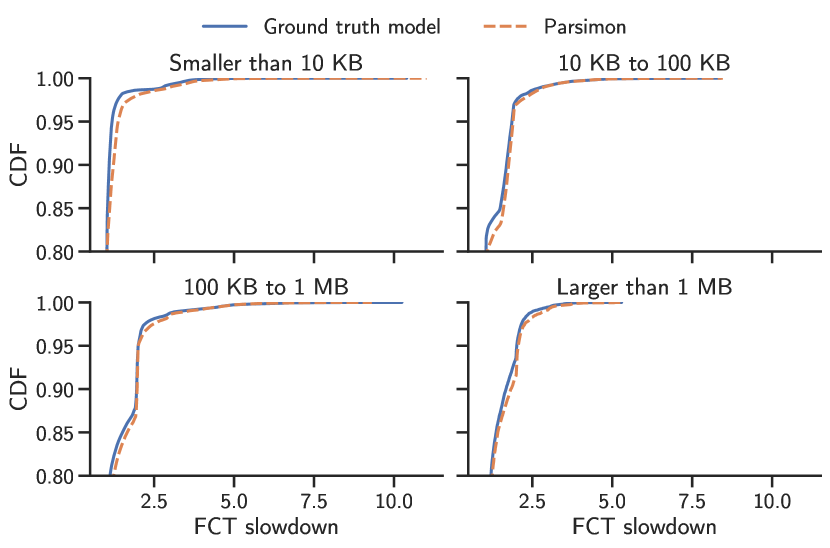
Figure 1. CDF of ns-3 versus Parsimon for flow completion time (FCT) slowdown across multiple flow size ranges, zoomed into the tail. While ns-3 took nearly 11 hours to produce these results, Parsimon took one minute and 19 seconds, end-to-end. Results were taken on a 6,144-host topology with an industry traffic matrix, 2-to-1 oversubscription, and bursty traffic.

We built Parsimon to directly test this hypothesis. First, we deconstruct the network topology into a large number of simple and fast simulations where each can be run entirely in parallel by a single hyperthread. Each simulation aims to collect the distribution of delays that flows of a particular size would experience through a single link, assuming that the rest of the network is benign. We then combine these simulated delay distributions to produce predictions of the end-to-end delay distribution, again for flows of a given size. At each step, we make conservative assumptions for how delays should be computed and combined. In many settings, researchers and operators are interested in keeping tail behavior well-managed, making a conservative assumption more appropriate than an optimistic one. Finally, Parsimon clusters links with common traffic characteristics, eliminating much of the overhead of simulating parallel links in the core of the network as well as edge links used by replicated or parallel applications, further improving simulation performance.

Because validation against detailed packet-level simulation at scale is so expensive, we focus our study on a single widely used transport protocol, DCTCP (dctcp, ), with FIFO queues with ECN packet marking at each switch (ecn, ). We also focus on queue dynamics rather than packet loss; most data center networks are provisioned and engineered for extremely low packet loss (fb-network, ; jupiter, ). We note that these assumptions are not fundamental to our approach. We show Parsimon generalizes to two other transport protocols, DCQCN (dcqcn, ) and the delay-based TIMELY (timely, ). Validation of other transport protocols (hull, ; homa, ; hpcc, ; swift, ), switch queueing disciplines (wfq, ; spfifo, ; homa, ; bfc, ), and packet loss remains future work. We note that modern data center transport layer protocols are adept at quickly adapting to the presence and absence of congestion, and so we caution our results may not extend to older transport protocols where convergence time is a large factor.

Parsimon speeds up simulations by reasoning about links independently, which enables massive parallelization, but at a cost in accuracy. As we will see in $\S$3.6, anything that creates standing congestion both at the core and at the edge, or when cross traffic is correlated across multiple hops, will result in less accurate estimates. While our methods are designed to favor overestimating rather than underestimating tail latencies, this property is only evaluated experimentally ($\S$5). In general there is no formal guarantee, since factors like congestion control can in theory behave in arbitrary ways that render less appropriate the approximation of considering links independently. We assume that we can simulate for long enough for the network to reach equilibrium; studies of short term transient behavior should not use our approach. We do not provide predictions at the level of an individual flow, but we are able to show that Parsimon is accurate for sub-classes of traffic for mixed workloads. We do not attempt to model end host scheduling delay of packet processing, even though that may have a large impact on network performance (tailtale, ; swift, ); we leave addressing that to future work.

To assess accuracy, we compare distributions of flow completion time (FCT) slowdown, defined as the observed FCT divided by the best achievable FCT on an unloaded network, and we say a flow is complete when all of its bytes have been delivered to its destination. Fig. 1 shows a sample of our results for the 6,144 host network mentioned above, running a published industry traffic matrix (fb-network, ) and flow size distribution (homa, ), and with standard settings for burstiness and over-provisioning. We describe the details of this and other experiments later in the paper. Depicted are FCT slowdown distributions binned by flow size. While ns-3 took nearly 11 hours on this configuration, Parsimon was able to match flow-size specific performance of ns-3 in 79 seconds (a 492 times speedup) on a single 32-way multicore server with an error of 9% at the 99th percentile. Given a small cluster of simulation servers, we estimate a completion time of 21 seconds using our approach.

In our evaluation, we scan the parameter space to identify circumstances where our approximations are less accurate. Link clustering improves performance but hurts accuracy somewhat; this tradeoff can be avoided by using more simulation cores. Without clustering, accuracy suffers when there is high utilization of links in the core (above 50%), there are high levels of oversubscription, and a large fraction of network traffic is due to flows that finish within a single round trip. Generally, a combination of factors is required for poor accuracy. In 85% of the configurations we test, the error relative to ns-3 is under 10%.

Parsimon source code and evaluation scripts are publicly available at https://github.com/netiken.

2. Parsimon Overview

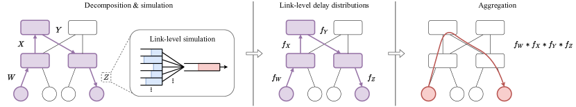
Figure 2. Overview of Parsimon. First, for any path, Parsimon estimates the contribution of each component link to delays in flow completion times, represented as a probability distribution. Parsimon then combines delays along the path using Monte Carlo simulation (see $\S$3). Further, for added performance, link-level simulations are optimized and redundant simulations (due to e.g., ECMP or symmetries in workload patterns) are pruned (see $\S$4).

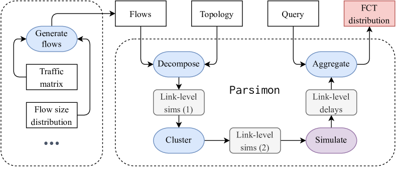
Figure 3. An illustration of Parsimon’s workflow. All inputs and outputs are shown in the top row. Rectangular boxes are inputs and outputs, rounded boxes are intermediate artifacts, and ovals are Parsimon’s actions.

This paper describes a set of methods to quickly and scalably estimate distributions of flow performance in data center networks. These techniques are implemented in a prototype called Parsimon, designed to provide the following:

• Fast, scalable estimates. We aim to supply estimates two to three orders of magnitude faster than full-fidelity simulation. Given enough cores, execution time should remain bounded regardless of network size.

• Tight latency bounds, including tail performance. Our approximations bias slightly towards overestimation, but still provide close estimates even for the 95th or 99th percentile of the distribution for a given flow length.

• Minimal restrictions on topology and workload. Our methods are largely independent of both topology and workload, although some combinations of topology and workload will have lower accuracy.

Fig. 2 illustrates the intuition behind its core method, and Fig. 3 depicts its workflow. The user supplies 1) a description of the topology, as a set of nodes and links, and 2) the workload, as a set of flows and routes. In our implementation, we generate the flow list by sampling from the traffic matrix and the flow size distribution, with inter-arrival times determined by a burstiness parameter. Once inputs are supplied, Parsimon proceeds in several steps:

Decomposition.   To start, flows are assigned to each link they traverse, e.g., for a fat tree using ECMP. Then, for each link $l$, Parsimon generates a custom backend simulation with a topology selected to determine—as accurately as possible—the contribution of $l$ to the end-to-end flow completion times (FCTs) of the flows passing through it. Each of these backend simulations can run in parallel.

Clustering.   Depending on the size of the topology, there may be tens or hundreds of thousands (or more) of link-level simulations to perform. Fortunately, data center topologies exhibit notable symmetries, and industry has reported that the same is true for many of their workloads (fb-network, ). Parsimon can optionally cluster links with similar workloads together. Only one representative from each cluster need be simulated; the rest of the link-level simulations are pruned. Clustering is discussed in more detail in $\S$4.2.

Simulation.   The next step is to simulate all cluster representatives in parallel. The decomposition step resulted in a topology and a workload for each link-level simulation, and we can use any simulation backend. Our prototype supports two: ns-3 and a custom high-performance link-level simulator ($\S$4.1). This allows us to directly validate our link-level simulator against ns-3. However, other efficient models, such as fluid flow (fluid, ) or machine learned models could be used here instead, for different tradeoffs of performance and accuracy. Each link-level simulation produces a distribution of the delay contributed by that link to the flow completion time (FCT), bucketed by flow size. Note this is not the link’s propagation delay—we calculate that contribution directly from the topology. These distributions—described in the next section ($\S$3)—are organized according to the original input topology, as depicted in Fig. 2. Recall that only one representative from each cluster is simulated; every other link is populated with the distributions of its cluster representative.

Aggregation.   The last step is to aggregate the link-level results into estimates for entire paths through the network. These estimates are also represented as delay distributions. Conceptually, Parsimon obtains a delay distribution for a path by convolving together the appropriate distributions from each of the path’s component links. Since there are multiple distributions per link and potentially many paths through the network, we do not compute convolutions up-front. Instead, convolution is done on-demand via Monte Carlo sampling; a by-product is that we can efficiently produce estimates for individual source-destination pairs, virtual networks, or classes of service ($\S$A). To make a single point prediction for a flow taking some path through the network, Parsimon uses the flow size to find the appropriate distribution for each link, samples a value from each of them, and combines them together. This process is repeated for each flow.

At a bird’s-eye view, Parsimon’s method is simple: to accelerate FCT estimates, we estimate the effect of each link independently and in parallel. Then to make predictions about the whole network, we combine the results. However in our experience, the accuracy of the method hinges tightly on the quality of the link-level estimates and subsequent aggregation. For example, when generating the backend simulations, we have observed that failure to adequately capture pertinent features of the network severely degrades the quality of Parsimon’s estimates. Similarly, link-level results must be processed and aggregated with care to preserve accuracy across all flow sizes. $\S$3 describes these techniques in detail.

3. Key Methods: Decompose and Aggregate

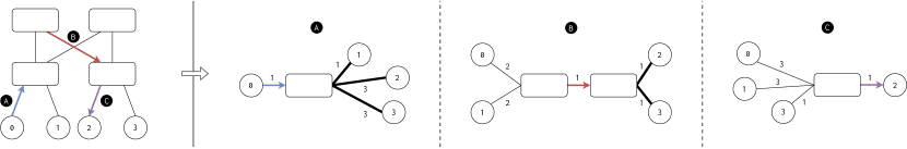
Figure 4. An illustration of how Parsimon generates link-level topologies. Simulations are unidirectional, and a different topology is used for (A) first-hop links, (B) switch-to-switch links, and (C) last-hop links. For illustration purposes, each link in the original topology has a propagation delay of one. To the left is the original topology; to the right are the corresponding link-level topologies, with new propagation delays annotated. Bold lines denote links whose bandwidths have been artificially increased during topology generation.

Together, the methods for decomposition and aggregation are what enables Parsimon’s scaling, and while we later engage additional techniques for further speed-up, they are a byproduct of—and not independent from—these more essential methods. Decisions made during this step are also the central determiners of accuracy. This section describes these processes in detail: how link-level topologies are generated, how the link-level data are post-processed and stored, and finally how they are aggregated to produce end-to-end estimates.

3.1. Generating Link-Level Workloads

To start, Parsimon associates each link with the flows passing through it. Since links are bidirectional, there are two sets of flows—and consequently two link-level simulations—per link. Parsimon populates links with flows using flows’ routes. Then for each link and in each direction, the associated flows constitute the input workload to the link-level simulation. The sizes and arrival times of the flows pass though unmodified.

3.2. Generating Link-Level Topologies

Once the link-level workloads are in place, we generate the link-level topologies. In this step, we think of each link as contributing some amount of delay to end-to-end FCTs. Any given flow will accrue these delays at each hop, depending on—for example—how much bandwidth is available and how much queueing is present. Highly-loaded links are expected to contribute more delay, while rarely utilized links will contribute relatively little.

For each link and in each direction, we generate a topology and perform a simulation using just the flows traversing that link. Once the simulation is finished, the delay caused by the link for a given flow is computed by taking the observed FCT and removing the ideal FCT for that flow size. (For a flow of size $s$ traversing a link of speed $C$ and propagation delay $l$, the ideal FCT is $s/C+l$.) This intuitively captures all delays incurred due to queueing, congestion control, bandwidth sharing, and so on at the target link.

In generating a per-link topology, our goal is to isolate and measure the expected delay contribution of the target link. A simple but inefficient strategy would be to use the original topology, but with only the traffic traversing the target link, without any cross traffic. This would be relatively accurate at measuring the delay contributed by the target link, albeit a bit conservative. Upstream cross traffic congestion will slightly smooth out downstream congestion at the target link, and so removing cross traffic would make the queue distribution at the target link slightly worse than in reality.

Although relatively accurate and parallelizable, simulating every link on the original network topology would still be inefficient, as packet-level simulation cost is roughly proportional to the number of packets simulated times the number of hops each packet takes through the network. Because we run the link simulation separately in each direction on every packet that passes through that link, this would inflate the aggregate computational cost of the simulation by a multiplicative factor of roughly half the average network path length—a significant factor for large-scale networks. Instead, we want to simulate only a small constant number of hops per target link.

An extreme alternative would be to simulate only the target switch queue. This is inaccurate for two reasons. First, we need to preserve end-to-end round trip delays, as these affect the speed of the congestion control adaptation to congestion or its absence; hosts closer to the target adapt faster than those farther away. Second, we need to preserve the spacing of packets induced by the original topology—a large flow does not immediately dump all of its data into the queue for the target link; instead, those packets arrive spaced apart by the edge link capacity. Ignoring this effect would lead to larger queues and more delay at the simulated link than would occur at that link in the original network.

Thus, we construct a topology for each link-level simulation that reflects a performance-accuracy tradeoff, attempting to capture the most important effects for computing the delay contributed by the target link. Fig. 4 shows how topologies are minimized. The generated topology takes one of three shapes, depending on the location and direction of the target link: (i) a first-hop up-link from a host to a ToR, (ii) a switch-to-switch link in the middle of the network, or (iii) a last-hop downlink from a ToR to a host.

Suppose the traffic through the target link originates from sources $S$ and terminates in destinations $T$. In case A of Fig. 4, we connect the target link directly to each host in $T$ via a dedicated link. If the target link is a switch-to-switch link (case B), we remove intermediate hops and connect the hosts in $S$ directly to the input, and the output directly to the hosts in $T$. Lastly, if the target link is a last hop (case C), then the hosts in $S$ are connected directly to the input. Rewriting the topology in this manner ensures that packets can traverse at most three hops, regardless of the size of the original topology.

Modeling round-trip delay.   Next, we set the link delays in each constructed topology to match the round trip delays in the original network. For example, in case A of Fig. 4, the round-trip time between host 0 and host 2 is 8 in both the original topology and the generated topology, even though Parsimon has removed intermediate hops between the switch and host 2. Fig. 4 is meant as illustrative; as with ns-3, Parsimon can model arbitrary round-trip delays.

In data center networks, congestion controllers play a large role in determining the extent to which longer flows yield throughput to benefit the latency of short flows. Most algorithms such as DCTCP (dctcp, ), DCQCN (dcqcn, ), and TIMELY (timely, ) are end-to-end in the sense that sources adjust their sending rates based on feedback echoed from destinations (bfc, ). With an end-to-end control loop, a source must wait an entire round-trip time (RTT) before being able to adapt its sending rate based on congestion feedback, resulting in longer queue lengths with higher RTTs. Thus, correctly modeling RTTs is essential to correctly modeling queue dynamics.

Selecting link bandwidths.   In some cases, we artificially increase the bandwidth of downstream links to ensure that they do not artificially add congestion. We say such links are inflated. For example, in cases A and B of Fig. 4, the bandwidths of the last-hop links are inflated. We want any queueing to be due to the target link and not the downstream link. By inflating downstream links, we remove store and forward delay (a small packet following a large packet would otherwise need to queue for the downstream link); it also addresses the case where core links are fatter than downstream links. Queueing at the downstream link itself is accounted for in case C. By contrast, we do not inflate first-hop links in cases B and C, as this would enable a long flow to arrive at the target link at a higher rate than it would in practice.

A cluster of sources sending simultaneously through an oversubscribed top-of-rack (ToR) switch in the original network will be throttled beyond what is implied by the edge link capacity. To improve simulation speed, we ignore this effect and are therefore slightly conservative in our estimates for oversubscribed networks.

Correcting for ACK traffic.   Since Parsimon only simulates one direction at a time, we must account for the load induced by acknowledgments due to traffic in the reverse direction. This is usually small, but can be significant at high load and where average packet size is small. Instead of modeling ACK traffic in detail, we apply a simple rule, mechanically reducing the forward bandwidth on each simulated link by the average volume consumed by ACKs for flows in the opposite direction over the course of the simulation. This correction is applied to all links but is most necessary for the target link. Note that Parsimon does not account for extra delay caused by ACK jitter on the reverse path; this could be an issue when applying our ideas to networks with bandwidth asymmetry between forward and reverse paths (reversepath, ).

3.3. Post-Processing Link-Level Results

Each link-level simulation produces an FCT for each flow in the link-level workload, and these FCTs are used to compute delays. Recall from $\S$3.2 that the delay is just the observed FCT minus the ideal FCT on an unloaded network. For each flow, we could, theoretically, estimate the end-to-end delay as some function of the delay contributed by each link for that flow. We discuss how that function works in Parsimon, along with its sources of bias, later in this section.

First, we address a different issue. Recall that we cluster similar links together ($\S$4.2) so that we only simulate the flows through a single representative link for each cluster of links. Thus, to compute the end-to-end delay for a particular flow, we take a sample from the delay distributions at each hop in the path, or from the hop’s standin representative.

In post-processing the link-level results and constructing these distributions, our primary objective is to support accurate estimates for all flow sizes. It is not enough to produce the correct FCT distribution across the entire workload; we must also accurately estimate the FCT distribution for short flows containing just a few packets as well as for long flows that last for hundreds of round trips. This extra requirement necessitates some post-processing before distributions can be constructed. Here we describe how this is done.

Packet-normalized delay.   Maintaining accuracy across all flow sizes would not be possible if we used delays directly. For example, long flows, which may experience variations in their bandwidth share over time, will almost always experience more absolute delay than short flows.

As a start, we can address this by normalizing delays by flow size: after computing the delay for a particular flow, we can then divide the delay by the flow’s size in packets. We call the resulting metric the packet-normalized delay, and it has the intuitive interpretation of summarizing the flow’s average delay per packet. Link-level distributions are constructed from packet-normalized delays rather than absolute delays. We normalize by the number of packets instead of the number of bytes because flows are discretized into—and therefore delays are incurred by—packets. Further, normalizing by the number of bytes loses accuracy for small flows, especially those smaller than the maximum packet size. For example, a 10 byte packet would be delayed by the same amount as would a 100 byte packet if it arrived in the switch queue just behind a jumbo (9 KB) frame (jumboframes, ).

Bucketing distributions.   Even with packet-normalized delays, we should still expect long flows to have different delay distributions than short flows. The FCT of a long flow is mainly determined by the throughput it achieves, while the FCT of a short flow depends on how much queueing it encounters. Further, congestion control algorithms trade the throughput of long flows for the latency of shorter ones to varying degree. An aggressive congestion control algorithm could try to keep queues near-empty (hpcc, ), resulting in smaller short-flow delay and larger long-flow delay.

To ensure that estimates for different flow sizes are accurate, it is necessary to sample each packet-normalized delay from the appropriate distribution. We bucket the distribution of packet-normalized delays by flow size. Buckets need to contain enough samples to form statistically meaningful distributions, but they should also be small enough so that the values come from flows with similar delay characteristics (i.e., similarly-sized flows).

Parsimon uses a simple bucketing algorithm. In brief, we start with a packet-normalized delay per flow, and we sort them according to flow size. Then, starting with the shortest flow, we begin populating buckets. For each bucket $b$, let $\text{maxf}_{b}$ and $\text{minf}_{b}$ be the maximum and minimum flow sizes associated with $b$, respectively, and let $n_{b}$ be the number of elements in $b$. Each bucket $b$ apart from the last one is locally subject to two constraints

$$n_{b}\geq B\qquad\text{and}\qquad\text{maxf}_{b}\geq x*\text{minf}_{b},\vspace{-1mm}$$

for some choice of $B$ and $x$. Globally, Parsimon also ensures buckets are contiguous and non-overlapping. For any bucket, once the two local constraints are satisfied, Parsimon begins populating the next bucket, and the final bucket is assigned whatever elements remain.

In practice, we find $B=100$ and $x=2$ works well. Data center workloads have heavy-tailed flow size distributions in which short flows arrive much more frequently than long ones. With these parameters, the first buckets will have size boundaries that are approximately powers of two, and as flows get larger, buckets will cover larger and larger ranges. This is the desired behavior. Intuitively, a queueing-sensitive 1 KB flow should not be grouped with a throughput-sensitive 1 GB flow, but a 1 GB flow can be grouped with a 10 GB flow provided the distribution of throughput is stable on long timescales. Accuracy across different flow sizes at finer or coarser resolution can be achieved by modulating $x$. We examined sensitivity to the number of buckets by decreasing $x$ for selected experiments and found no meaningful change in the predicted distributions.

In summary, each link-level simulation produces FCTs, and these FCTs are used to construct bucketed distributions of packet-normalized delay. Since different links have different workloads, bucketing is performed on a per-link basis. This means that the links in any given path are likely to have different bucket sizes with different flow size ranges. In the next subsection ($\S$3.4) we describe how the data are aggregated.

3.4. Aggregating Link-Level Estimates

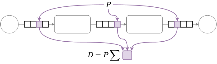
Figure 5. An illustration of how Parsimon aggregates link-level results into a path-level point estimate. Parsimon samples a packet-normalized delay ($\S$3.3) from each link along the path, and combines these to estimate the end-to-end absolute delay $D$.

For any given range of flow sizes, the final distribution of (packet-normalized) delay for any path through the network can be estimated by selecting an appropriate distribution from each component link and then performing an n-ary convolution. However, the efficiency of this step must be considered. Since there are multiple distributions per link and potentially many paths through the network, performing all convolutions up front and storing one path-level distribution per path, per flow-size range would be costly in space and in time.

To avoid these costs, Parsimon uses an on-demand sampling strategy to perform the convolution. Recall that the simulation step resulted in bucketed distributions of packet-normalized delay per link, organized in a graph isomorphic to the original topology. Parsimon makes this graph a queryable object that is capable of supporting point estimates. Given a size, a source, and a destination, Parsimon computes a path from the source to the destination and uses the size to select a distribution per-link. Then, one packet-normalized delay is sampled from each distribution and the results are subsequently combined into a point estimate. Suppose there are $n$ hops and let $D^{*}_{1},D^{*}_{2},\ldots,D^{*}_{n}$ be the sampled packet-normalized delays. Then, the end-to-end absolute delay $D$ is computed as

$$P\sum_{i=1}^{n}D^{*}_{i}\enspace=\enspace\sum_{i=1}^{n}D^{*}_{i}P\enspace=\enspace\sum_{i=1}^{n}D_{i}\enspace=\enspace D,\vspace{-1mm}$$

where $P$ is the input flow size in packets and $D_{i}$ is the absolute delay for hop $i$. Fig. 5 illustrates this process. Finally, to obtain a distribution of end-to-end delay estimates, we need only sample enough point estimates for the desired flow size range and source destination pairs.

3.5. Primary Source of Speedup

Parsimon speeds up large network simulations by considering the effect of each link in isolation, allowing it to scale in the size of the simulated network and the number of processing cores. Although the link is the unit of decomposition, Parsimon’s scaling ability is determined not by the total the number of links, but rather by the fraction of total packets traversing any link. In other words, Parsimon’s speed-up depends on the number of busy links and how well the load is balanced among them. This explains why Parsimon is most suited for large data center networks, where the total workload comprises many source destination pairs with many paths between them. If a network traffic is heavily skewed such that most of the workload traverses only a few paths, the amount of speedup will be limited.

3.6. Primary Sources of Error

To balance accuracy and performance, Parsimon makes a number of approximations, with some having more of an effect on accuracy than others. Here we catalog some of the main sources of error, describing 1) how we expect the errors to manifest and 2) what modifications, if any, could be made to address them.

Bottleneck fan-in.   To simulate a given target link in the network, Parsimon constructs a topology that connects all of the source nodes feeding traffic directly into that target. In practice, of course, there would be multiple stages of fan-in, and that fan-in would tend to spread out any burst of arriving flows due to upstream bandwidth capacity constraints. Any target link would experience slightly less queueing and less congestion in reality than in Parsimon. Of course, Parsimon also simulates the upstream link; because it is closer to the sources, its traffic and queueing behavior would be a closer model to what would happen in a full network-wide simulation.

Because Parsimon sums the delay contributed by each hop along a flow’s path, the lack of fan-in will tend to slightly overestimate the delays caused by downstream links. Put another way, any delay induced by fan-in constraints is counted twice—once when we simulate the upstream link and again when we simulate the downstream link. In our evaluation, accuracy is slightly lower for networks with higher degrees of oversubscription, as we would expect. We could potentially remove this inaccuracy by including the upstream fan-in as part of the topology for each link simulation. Since simulation time is proportional to the number of hops, this would decrease individual link simulation efficiency by a small but significant factor.

Lack of traffic smoothing.   Similarly, any cross-traffic that shares a portion of a path with traffic destined for the target link will tend to smooth out traffic before it reaches the target. Parsimon does not include any cross-traffic in its per-link simulation, making it slightly overestimate the queueing delay at the target link. Assuming the simulation is stable—that the arrival rate does not exceed the service rate for any link—the target link will experience the correct long-term average rate, but without as much smoothing as would happen in practice. We see evidence of this effect in our evaluation, where error is slightly larger for workloads with a predominance of short flows which would benefit more from smoothing. Of course, correctly modeling the effect of cross-traffic on the traffic arriving at a downstream link would be difficult to accomplish without reverting to a full network simulation.

Link-level independence.   A more fundamental approximation is that link-level simulations are treated independently. This technique enables wholesale parallelization, but its accuracy depends on the amount of correlation between the traffic intensities on the various hops along the path. The more correlated the traffic, the more error Parsimon’s method produces.

Since Parsimon produces estimates by convolving delay distributions (adding independent random variables), full accuracy requires the mutual independence of delays among the links in every path. Consider a single-packet flow that traverses two hops, both with load $l$. If the delays along the two hops are independent, the probability that the flow will encounter no queueing is simply $(1-l)^{2}$. However, if both hops tend to have queueing at the same time (i.e., if the traffic intensities and therefore the delays are correlated), then that probability is closer to $1-l$. Since Parsimon does not distinguish between these two scenarios, the difference is not reflected in its estimates.

In very large networks with thousands of hosts and paths, and with realistic workloads, we expect the effects of correlation to be small. A basic result of queueing theory is that under some circumstances it is possible to analyze queues independently, even when the output of one queue connects to the input of another, so that queue behaviors are obviously correlated. One view of our work is that we are empirically observing that data center networks approximately admit product-form solutions for their equilibrium state queue distributions under realistic workloads.

However, some networks use PFC (dcqcn, ) to reduce packet loss due to go-back N error handling in some RDMA network interface cards. Because PFC suffers from head-of-line blocking, PFC can cause correlated congestion across multiple links, and so Parsimon would not be a good choice for modeling such networks. If correlation is a problem, we could potentially measure the degree of correlation and apply a correcting factor during the convolution step, but we leave that for future work.

One bottleneck at a time.   Estimating the performance of long flows comes with an additional difficulty which is also exacerbated by correlated delays. While a single packet flow can only reside in one queue at a time, a long flow can be backlogged on multiple links at the same time. Depending on the specific congestion control mechanism, the throttling back of a long flow (the delay it experiences) is typically not the sum of the delays it would experience on individual links (as Parsimon approximates), but rather only the delay caused by the true (instantaneous) bottleneck. Since Parsimon sums all delays, it will overestimate the end-to-end delay for the long flow that encounters simultaneous cross-traffic congestion at multiple points along its path. In summary, Parsimon is more accurate when the congestion is episodic and temporary, appearing at different links at different times, and less accurate when congestion is persistent across multiple edge and core links of a given path.

Congestion on any link (and therefore simultaneous congestion on multiple links) becomes more common with higher network load, and we see this effect in our evaluation. We can potentially correct for this bias by using a more complex function for combining link delays when overall network utilization is high. Because network operators are often willing to over-provision their network hardware to reduce application tail latency, this is rare in practice. For example, some recent end-to-end congestion protocols, such as Homa (homa, ), simply assume that network congestion predominantly occurs at the last hop of each path. We do not make such an assumption; we handle congestion equally wherever it might occur. However, we do assume that congestion events are not persistent and network wide.

Our approximations are biased toward producing overestimates rather than underestimates, because we expect network operators to be more sensitive to over-promising tail behavior, even if that comes at the cost of being too conservative with respect to capacity planning. Additional analyses on the errors induced by these approximations can be found in the appendix ($\S$C).

4. Complementary Methods

The previous section described how we decompose a single large network simulation into many small, independent ones that can be executed in parallel and later combined. This section describes additional optimizations that reduce, cluster, and prune these link-level simulations for better computational efficiency. These reduce the number of cores needed to simulate a given network within some time bound, or equivalently, the execution time on a single server machine.

4.1. Fast Link-Level Simulation

By far the largest computational cost in Parsimon are the link-level simulations. Initially we used ns-3 as our link-level backend. However, as a general-purpose simulator, ns-3 is designed to support arbitrary protocols with arbitrary extensions, all the way down to hardware models. This is more flexible but means that every packet in ns-3 generates events at every host, queue, and link—as well as throughout the hosts’ modeled network stacks.

Instead, we implemented a custom and minimal simulator optimized for high fidelity single link simulation. This backend only models the workload, topology, queueing, and congestion control. For congestion control, our prototype implements DCTCP’s core algorithm (dctcp, ) in a few tens of lines of code. For example, we do not need to model the mechanism for carrying ECN bits from switches back to endpoints. Switching to a custom simulator speeds up the individual link simulations by roughly an order of magnitude, with negligible loss of accuracy. Reducing the simulation time of the worst case (most congested) link also reduces the critical path dramatically. If more simulation features are needed, Parsimon can use ns-3 at the cost of using more cores.

4.2. Clustering and Pruning Simulations

Algorithm 1 Greedy link clustering

1:unclustered $\leftarrow$ AllLinks $\triangleright$ links here are unidirectional

2:clusters $\leftarrow$ [] $\triangleright$ list of list of links

3:while not Empty(unclustered) do

4:    members $\leftarrow$ [] $\triangleright$ new cluster

5:    representative $\leftarrow$ PopFirst(unclustered)

6:    Push(members, representative) $\triangleright$ with initial member

7:    for candidate in unclustered do $\triangleright$ find other members

8:         rfeature $\leftarrow$ Feature(representative)

9:         cfeature $\leftarrow$ Feature(candidate)

10:         if IsCloseEnough(rfeature, cfeature) then

11:             Push(members, candidate) $\triangleright$ new member

12:             Remove(unclustered, candidate)              

13:    Push(clusters, members)

14:return clusters

Lastly, we recall that Parsimon’s decomposition results in two simulations per link: one in each direction ($\S$3.1). On a large-scale 6,144-host topology we use for evaluation, there are over 9,000 links, and therefore over 18,000 simulations generated. Fortunately, data center topologies commonly induce symmetries that render some of these simulations redundant. For example, up-links in the same ECMP grouping can be assumed to have the same characteristics and traffic patterns. Furthermore, the workloads themselves may also induce symmetries due to communication patterns and load balancing (fb-network, ).

We can take advantage of these symmetries by clustering links that carry similar traffic and only simulating one representative from each cluster. Then, in each cluster, all links inherit the delay distribution produced by the representative link. Parsimon’s clustering requirement is quite specific, which limits the range of popular clustering algorithms that can be used. Let $l_{1},l_{2}\in L$ be any two link-level simulations, and let $d:L\times L\rightarrow\mathbb{R}$ be a distance function. Ideally,

$$l_{1}\text{ and }l_{2}\text{ are clustered together}\iff d(l_{1},l_{2})<\epsilon,\vspace{-1mm}$$

where $\epsilon$ is some bound. The left-to-right direction preserves accuracy; the right-to-left supports efficiency. Most centroid-based and density-based clustering algorithms aren’t designed to provide the left-to-right property. Instead, Parsimon uses Alg. 1. This algorithm greedily clusters simulations together, using a distance function that predicts which links will have similar delay profiles. In our prototype, we check that the link flow size and inter-arrival time distributions—as well as their load levels—are close. We find this provides a reasonable tradeoff between efficiency and accuracy, but users can turn off the optimization at the cost of using more cores. Further details about the clustering can be found in the appendix ($\S$D).

5. Evaluation

Parsimon’s goal is to quickly estimate tail latencies for a variety of large data center networks and workloads. In evaluating Parsimon, we would like to assess 1) Parsimon’s accuracy and performance at the scale of thousands of hosts, and 2) how accuracy is affected by a wide range of variables over the workload and the topology.

Our strategy is as follows. Using workloads extracted from industry datasets, we start with a 384-rack, 6144-host topology to evaluate Parsimon’s speed and accuracy in one scenario at scale. Then, to evaluate nearly 200 other topology and workload scenarios, we downsample the workload so that it can run on a smaller 256-host topology. This allows us to run enough ns-3 simulations quickly enough to perform a detailed sensitivity analysis.

To more clearly illustrate sources of error in Parsimon, we also construct and evaluate Parsimon on synthetic workloads on a small-scale parking lot topology in Appendix $\S$C.

5.1. General Setup

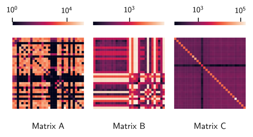
(a) Traffic matrices (32-rack sample)

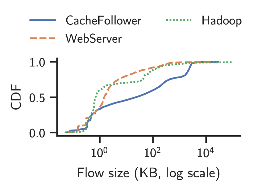
(b) Flow size distributions

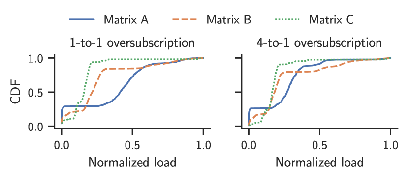
(c) Normalized link load distributions

Figure 6. In the evaluation, we model workloads using data from Roy et al.’s study of Meta’s data center network (fb-network, ). The traffic matrices in Fig. 6(a) are extracted from the accompanying dataset, and the flow size distributions in Fig. 6(b) are estimated from the published data. Lastly, for a given topology, the distribution of link loads depends on 1) the traffic matrix and 2) the degree of oversubscription. Fig. 6(c) shows the link loads induced by the matrices in Fig. 6(a) on two 32-rack topologies with different overprovisioning. The x-axis is normalized to the maximum link load.

Variant	Clustering?	Link-level backend
Parsimon	No	custom
Parsimon/C	Yes	custom
Parsimon/ns-3	No	ns-3
Parsimon/inf	—	custom

Table 1. The Parsimon variants under consideration. Parsimon/inf is a variant that assumes infinite cores and memory.

Each scenario we consider has six components: 1) a topology size, 2) an oversubscription factor, 3) a traffic matrix, 4) a flow size distribution, 5) a burstiness level, and 6) a maximum load level. Here, we briefly describe how these are specified and configured. We also discuss which Parsimon variants we will assess and how we establish a baseline.

Topology and oversubscription.   To mimic an industry topology, our topologies are modeled after Meta’s data center fabric (fb-fabric, ). In brief, there are three layers of switches: hosts connected to a top-of-rack switch (ToR) with 10 Gbps links constitute a rack, racks connected to each other via fabric switches with 40 Gbps links constitute a pod, and pods connected to each other via spine switches with 40 Gbps links constitute a cluster. Spine switches are organized in planes. We can modulate the size of a topology (corresponding to a cluster) by adjusting the number of pods, the number of racks per pod, and the number of hosts per rack, and we can modulate the oversubscription factor by adjusting the number of spines per plane.

Traffic matrices.   The traffic matrices are extracted from the datasets accompanying Roy et al.’s study of Meta’s data center network (fb-network, ). The data only allow us to construct reliable rack-to-rack matrices. When sampling workloads, we use the matrices to generate rack-to-rack traffic, but once a rack is chosen, we select its hosts uniformly at random. This may bear semblance to reality: according to Roy et al., Meta’s racks typically only contain servers in the same role, and load balancing is used pervasively. We use traffic matrices from three different clusters: a database cluster (matrix A), a web server cluster (matrix B), and a Hadoop cluster (matrix C). Fig. 6(a) shows 32-rack samples of the matrices.

Flow sizes and burstiness.   We use three flow size distributions, estimated from published data in Roy et al.’s study (fb-network, ). These are reproduced in Fig. 6(b). For inter-arrival times, we use the log-normal distribution to model bursty traffic, and we modulate the burstiness by adjusting the log-normal shape parameter $\sigma$. For low burstiness, we select $\sigma=1$, and for high burstiness, we choose $\sigma=2$.

Maximum load level.   When setting a load level, we ensure that the offered rate is less than the link capacity for each link by specifying the maximum load level that any link can have. Note that a given maximum load level may result in different link load distributions, depending on the traffic matrix and the topology. Fig. 6(c) shows the distribution of normalized link loads on a 32-rack topology with the traffic matrices in Fig. 6(a) and two different oversubscription factors. When describing how loaded a topology is, we will usually specify the average load of the top 10% most loaded links.

Parsimon variants and baseline.   To establish a baseline for Parsimon’s accuracy and performance, we use ns-3 with the optimized build profile. We also consider several Parsimon variants, summarized in Table 1. By default, Parsimon uses the custom link-level backend ($\S$4.1) with clustering turned off. This expresses a lower bound on Parsimon’s expected speed-up given a particular machine. Parsimon/C adds clustering to the default variant using the methods described at the end of $\S$4.2, and Parsimon/ns-3 replaces the default’s custom backend with ns-3. Lastly, Parsimon/inf provides an estimate of Parsimon’s performance given infinite cores and infinite memory, computed by adding the run time of the longest link-level simulation to the fixed costs of network setup and convolution sampling. This represents an upper bound on the Parsimon’s achievable performance. All performance measurements are taken on a 32-core AMD Ryzen Threadripper 3970X.

5.2. Analysis on a Large-Scale Network

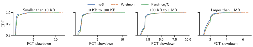
Figure 7. CDFs of FCT slowdown estimated by ns-3 and two Parsimon variants (note the y-axis). On a large network with 6,144 hosts, an industry traffic matrix (matrix B), and 2-to-1 oversubscription in the core, Parsimon’s latency estimates are similar to those produced by full-fidelity simulation. Table 2 shows the performance of each estimator.

Estimator	Time	Speed-up
ns-3	10h 48m 26s	—
Parsimon	4m 13s	$154\times$
Parsimon/C	1m 19s	$492\times$
Parsimon/inf	21s	$1864\times$

Table 2. Running times and speed-up of Parsimon variants for five seconds of simulated time on a large oversubscribed network with thousands of hosts. We find that Parsimon estimates latencies orders of magnitude faster than does ns-3. If there is ample opportunity for clustering or if there are infinite compute resources, speed-up is substantially further increased. Measurements were taken on a 32-core machine.

Here we evaluate Parsimon’s accuracy and performance on a 384-rack, 6144-host topology. The topology has eight pods, 48 racks per pod, and 16 hosts per rack, with 2-to-1 oversubscription. For the workload, we use matrix B, the WebServer flow size distribution, and high burstiness ($\sigma=2$). We set a maximum link load of about 50%, which gives the 100 most loaded links an average load of 32%, and the top 10% most loaded links an average load of about 15%. We configure all simulations to run for five seconds of simulated time. To establish a baseline, we first run the scenario in ns-3, then we run the scenario in Parsimon and Parsimon/C (see Table 1). Due to memory constraints we omit Parsimon/ns-3 here, but we include its analysis at smaller scale in $\S$5.3.

Fig. 7 shows the accuracy of Parsimon relative to ns-3 across four flow size bins. We find that across all bins, both variants accurately estimate tail latencies. If we consider all flow sizes together, we find that Parsimon and Parsimon/C overestimate the p99 FCT slowdown by 8.8% and 7.5%, respectively.

Table 2 shows the running time and speed-up for each estimator, which includes topology generation and convolution sampling overheads where applicable. While ns-3 took nearly 11 hours, Parsimon without clustering took four minutes and 13 seconds, for a speed-up of $154\times$. If we turn clustering on by using Parsimon/C, the running time is further reduced to one minute and 19 seconds, for a speed-up of $492\times$. In this case, only 25% of links were simulated; the rest were pruned. Lastly, Parsimon/inf estimates Parsimon’s best possible performance given infinite compute resources. The longest-running single-link simulation took 11 seconds, and with the additional 10 seconds required for network setup and convolution sampling, the fastest projected running time is 21 seconds.

We chose an oversubscribed topology to slightly disadvantage Parsimon’s method, as oversubscription can lower Parsimon’s accuracy. $\S$5.3 analyzes the effect of oversubscription in more detail. We also ran the above experiment on a topology without oversubscription, which for the same maximum load setting increased the top 10% average link load from 15% to 25%. We found Parsimon’s p99 accuracy improved from 9% to about 7%, while Parsimon/C’s accuracy remained approximately the same. However, because aggregate load increased, ns-3 took 27 hours for five seconds of simulated time, and speed-ups for Parsimon, Parsimon/C and Parsimon/inf were $152\times$, $872\times$, and $3487\times$, respectively. Parsimon/C benefited from the increased number of links in each ECMP grouping, allowing it to prune 85% of the link-level simulations.

5.3. Sensitivity Analysis at Small Scale

Parameter	Sample space
Oversubscription	1-to-1, 2-to-1, 4-to-1
Traffic matrix	Matrix A, Matrix B, Matrix C
Flow size distribution	CacheFollower, WebServer, Hadoop
Burstiness	Low ($\sigma=1$), High ($\sigma=2$)
Max load	26% to 83% (continuous range)

Table 3. The sample space for the sensitivity analysis in $\S$5.3.

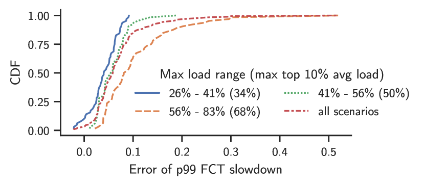
Figure 8. CDFs of p99 error between Parsimon and ns-3 across all scenarios drawn from the sample space in Table 3. The distributions are binned by maximum load. In parentheses, we give the maximum value for the top 10% average load in each bin. Under common conditions of low to moderate load, Parsimon’s estimates for the p99 FCT slowdown are reliably within 10% of the ground truth.

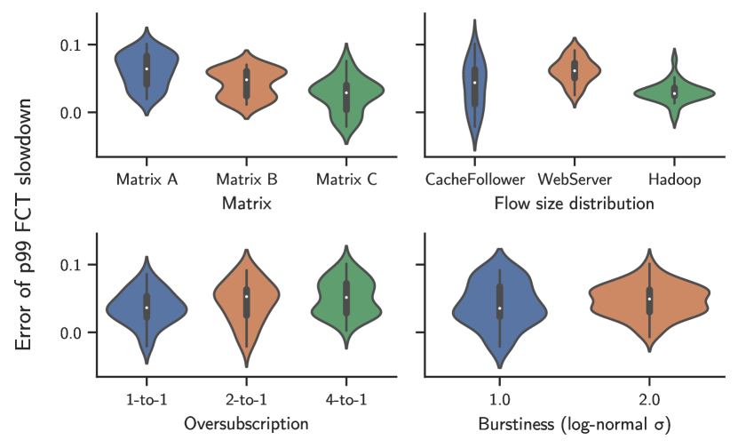
(a) Max load $\leq$ 50%

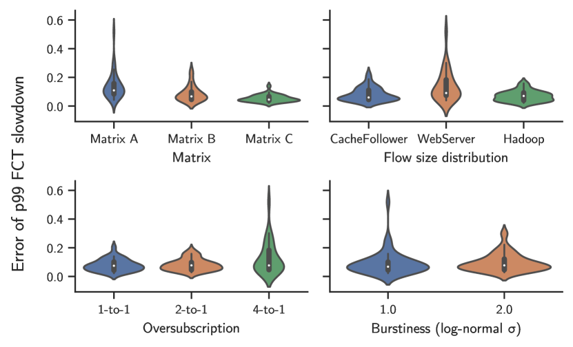
(b) Max load $>$ 50%

Figure 9. Distributions of p99 error between Parsimon and ns-3, faceted by different workload and topology parameters. For each distribution we show the median, the quartiles, and a rotated kernel density estimation. We consider the low-load regime (Fig. 9(a)) and the high-load regime (Fig. 9(b)) separately. At low load, the workload and topology parameters only have a modest effect on Parsimon’s accuracy, but at high load, the conditions leading to the largest errors come into view: high load, high oversubscription, with very short flows. Note the different y-axes between the two load regimes.

Next we turn our attention to how different aspects of workloads and topologies affect Parsimon’s accuracy. To be able to simulate enough scenarios in ns-3 for a sensitivity analysis, we downsample the topologies and traffic matrices to 32 racks. The resulting topologies have two pods, 16 racks per pod, and eight hosts per rack, and the number of spines per plane varies to accommodate different oversubscription factors.

Our approach is as follows. First, we construct a sample space over the parameters defining the workload and the topology (aside from the number of servers, which is fixed). The sample space is shown in Table 3. Then, we sample 192 scenarios uniformly at random, and we run ns-3 and the default Parsimon variant on each of them for several seconds of simulated time. Next, for each scenario, we take the p99 FCT slowdown estimated by both ns-3 and Parsimon, and we compute the error between them. If these values are $n$ and $p$ respectively, then the error is $(p-n)/n$. Negative values indicate that Parsimon produced an underestimate.

Since we have one error value per scenario, the errors give rise to distributions of error associated with the original sample space. Now what remains is to determine how the workload and topology parameters affect error distributions. To start, recall from the discussion in $\S$3.6 that the magnitude of error is expected to be load-dependent, with higher errors typically manifesting at higher loads, so we begin by examining the effect of the maximum load setting on Parsimon’s accuracy.

Maximum load.   Fig. 8 shows the error distributions binned by maximum load. Among all scenarios, Parsimon’s p99 estimates are within 10% of ns-3’s estimates 85% of the time At high load, we observe larger overestimates of up to 52% in the worst case. In the most highly-loaded group of scenarios—with maximum link loads between 56% and 83%—Parsimon is within 10% of ns-3 62% of the time, with an average error of about 11%. However, this includes scenarios where 10% of the links have an average load of up to 68%, which is much higher than what is reported in the literature. For example, Roy et al. report that in Meta’s data center network, 99% of host links are less than 10% loaded, and the top 5% of core links have loads between 23% and 46% (fb-network, ). Among scenarios where the maximum link load is between 26% and 41%, Parsimon is within 10% of ns-3 100% of the time. If we further include scenarios with maximum link loads between 41% and 56%, that number falls to 96%. Finally, while Parsimon’s techniques tend to overestimate latencies, in 3% of the scenarios, Parsimon underestimates p99 slowdown by up to 2%.

Error	Max load	Matrix	Sizes	Oversub	$\sigma$
51.9%	77.6%	A	WebServer	4-to-1	1
30.1%	67.3%	A	WebServer	4-to-1	2
29.6%	67.0%	A	WebServer	4-to-1	2
25.6%	65.9%	A	WebServer	4-to-1	1
24.6%	73.2%	B	WebServer	4-to-1	1

Table 4. The five scenarios with the highest error values from the sensitivity analysis in $\S$5.3.

Other parameters.   We next turn to the effects of all other workload and topology parameters. We start by only considering scenarios where the maximum link load is less than or equal to 50%; this will tell us whether any of the parameters have a large effect on accuracy in the low-load regime. Fig. 9(a) shows the median error and error distributions as a violin plot for low-load scenarios grouped by traffic matrix, flow size distribution, oversubscription, and burstiness. Overall, changes to these parameters appear only to have a modest effect. The choice of traffic matrix has the clearest trend, but load is a confounder here: recall from Fig. 6(c) that different traffic matrices yield different link load distributions for the same maximum load setting.

When we look at the high load regime in Fig. 9(b), a clear picture comes into view. We see much longer tails in error distributions for matrix A, the WebServer flow size distribution, and 4-to-1 oversubscription. Together with Fig. 9(a), this suggests that none of these settings has a strong effect on its own, but coupled together in the high load regime, they have a pronounced effect on Parsimon’s accuracy. Matrix A induces higher average load and has more cross-rack traffic, making it more likely for its flows to encounter multiple simultaneous bottlenecks. The WebServer flow size distribution is dominated by short flows (Fig. 6(b)), a third of which are smaller than 1 KB and 80% of which are smaller than 10 KB. Because more of the traffic completes within a single round trip, there is more ephemeral congestion and bandwidth smoothing can have a larger impact.

Finally, oversubscription has an effect at high load: if we removed all scenarios with 4-to-1 oversubscription, the maximum error would only be 20% rather than 52%, even at high load. In addition to the double counting of delays described in $\S$3.6, oversubscription can also increase correlations in link delays. To achieve 4-to-1 oversubscription in topologies as small as these, there are only four spine switches per plane forwarding traffic between groups of 16 racks, leaving relatively few paths through the core. Fewer paths can result in higher degrees of correlation—especially with matrix A, whose traffic is primarily inter-rack (Fig. 6(a)). Finally, this setting combined with the short flows from the WebServer distributions gives rise to errors of up to 52%.

Table 4 lists the scenarios with the top five highest error values. Four have matrix A, all have the WebServer distribution, and all five have 4-to-1 oversubscription. In this group, the average maximum load is 70.2%. Since we expect the combination of all-to-all workload, heavily oversubscribed topology, and persistently high core utilization to occur relatively infrequently, the data suggest that Parsimon maintains good accuracy under common conditions.

Mixed Workloads.   We also use the small topology to study the Parsimon prediction error for subsets of traffic in heterogeneous workloads in Appendix $\S$A.

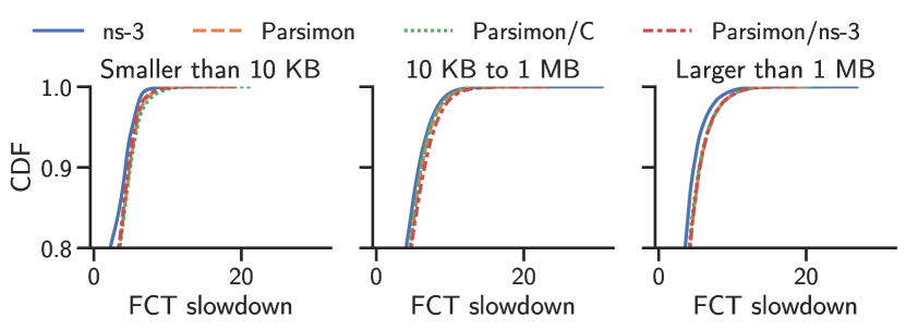
Figure 10. CDFs of FCT slowdown estimated by ns-3 and Parsimon for the scenario whose error is at the 85^th percentile of the p99 error distribution. Note the y-axis. Even though the accuracy here is worse than in the common case, Parsimon’s estimates remain close across most of the tail. Also shown is Parsimon/ns-3.

5.4. Analysis of One Configuration

We pick one representative scenario to examine in more detail, to test if our approach is robust to alternate definitions of tail latency, congestion control protocol, workload, and topology. To pick a scenario whose accuracy is somewhat worse than the average case, we rank-order all scenarios by error and select the one at the 85^th percentile. This has matrix A, the Hadoop flow size distribution, low burstiness, 2-to-1 oversubscription, and a maximum load of 68% (with a top 10% average load of 56%).

Tail distribution.   Operators may differ in their definitions of tail latency, e.g., focusing on the 90th or 99.9th percentile, rather than just the 99th FCT slowdown. Fig. 10 shows the tail of the cumulative distribution of FCT slowdown for different flow sizes for the selected configuration, for ns-3 and each of the Parsimon variants. The prediction error is similar across the tail of the distribution for this scenario, with little accuracy difference between any of the variants.

Protocol	Max load	Error in p99 FCT slowdown
		¡ 10 KB	10 KB - 1 MB	¿ 1 MB
DCTCP	45%	1.4%	9.2%	15.9%
TIMELY	45%	4.0%	17.9%	13.7%
DCQCN	45%	5.9%	11.6%	12.8%
DCTCP	56%	2.8%	9.2%	14.6%
TIMELY	56%	8.1%	20.0%	11.3%
DCQCN	56%	7.6%	14.6%	12.2%
DCTCP	67%	13.8%	11.3%	13.6%
TIMELY	67%	13.3%	18.2%	5.0%
DCQCN	67%	18.0%	15.2%	13.6%

Table 5. Prediction error of Parsimon/ns-3 for estimated p99 FCT slowdown with three different congestion control protocols for the sample configuration at different load levels and for different request sizes.

Transport protocols.   We use the sample scenario to test the generality of Parsimon to two additional congestion control protocols, DCQCN (dcqcn, ) and TIMELY (timely, ). DCQCN is designed for RDMA traffic, while TIMELY uses network delay, rather than ECN signals, to detect congestion. To focus on prediction error for our approximation methods, we use the pre-existing ns-3 implementation of the protocols as the Parsimon link level simulator for this part of the evaluation. Note that Parsimon and Parsimon/ns-3 exhibit a few percent difference in p99 error for DCTCP for this configuration. Because the prediction error for different congestion control protocols may depend on the amount of congestion, we also run the experiment at varying load levels.

Table 5 shows the prediction error for Parsimon/ns-3 relative to ns-3 in the estimated p99 FCT slowdown at three load levels for the three transport protocols, aggregated by request size. For this configuration, Parsimon is most accurate for small flows and low to moderate maximum link utilization, and that is true for all three congestion control protocols. DCTCP has somewhat lower error for small and medium size flows at low to moderate utilization. Relative error is higher for larger transfers and higher maximum link utilization, with no clear pattern in the error for different protocols.

Simulated link failures.   We also use the sample configuration to examine the prediction accuracy for topologies with simulated link failures in Appendix $\S$B.

6. Conclusion

In this paper, we propose and evaluate a new method for computing a conservative estimate of flow-level tail latency for large scale data center networks, given an arbitrary traffic matrix, topology, flow size distribution, and inter-arrival process. Our approach decomposes the problem into a large number of individual link simulations, specially constructed to produce accurate estimates of the probability distribution of delay contributed by congestion at each link. We then mechanically combine these link-level delay distributions to produce flow-level estimates. On a large-scale network using a commercial workload, our approach outperforms ns-3 by a factor of 492 on a single multicore server with a loss of accuracy of less than 9% in the tail of the latency distribution.

Acknowledgments. We are grateful to Vincent Liu, Jeff Mogul, our shepherd Arpit Gupta, and the anonymous reviewers for their feedback and useful comments. This work was supported in part by NSF grants CNS-2006346, CNS-2006827, a Cisco Research Center Award, and a Google Research Award.

Appendix A Mixed Workloads

Parsimon’s methods are designed to estimate performance distributions rather than per-flow metrics. However, it is often useful to aggregate FCT performance estimates in different ways. For example, an operator may wish to estimate the performance of individual virtual networks or individual services. In this section, we conduct a simple experiment to assess Parsimon’s ability to estimate performance for separate aggregates.

We start by mixing three different workloads—each with its own traffic matrix and flow size distribution—into one workload. Table 6 summarizes their differences. Each workload has a maximum load setting of 20% and a high burstiness setting ($\sigma=2$), and their combination results in a maximum link load of about 50%. We run the combined workload on the small-scale topology with 2-to-1 oversubscription from $\S$5.3, and we observe the accuracy for each workload faceted by flow size. Fig. 11 shows the cumulative distribution function (CDF) of FCT slowdown for ns-3 and Parsimon. We observe that across all workloads and flow size bins, Parsimon maintains good accuracy.

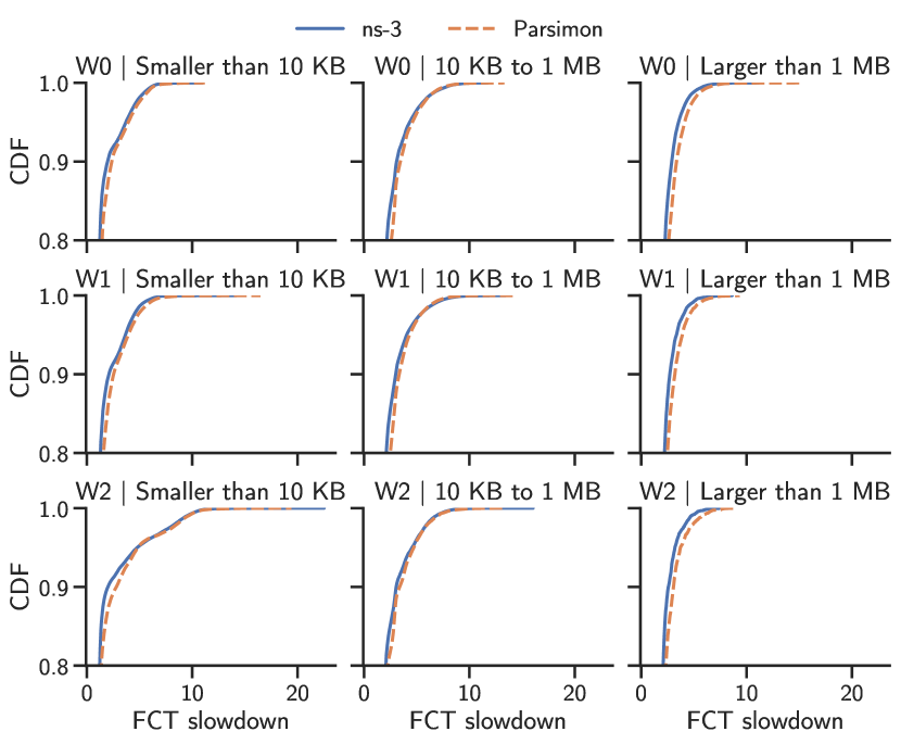
Figure 11. CDFs of FCT slowdown for ns-3 and Parsimon, bucketed by workload and flow size. Note the y-axes. When mixing workloads in a single simulation, Parsimon can accurately estimate performance distributions for individual workloads in addition to full-network aggregates.

Name	Matrix	Sizes	Max load	$\sigma$
W0	A	CacheFollower	~20%	2
W1	B	WebServer	~20%	2
W2	C	Hadoop	~20%	2

Table 6. The three workloads mixed together in $\S$A.

Appendix B Link Failures

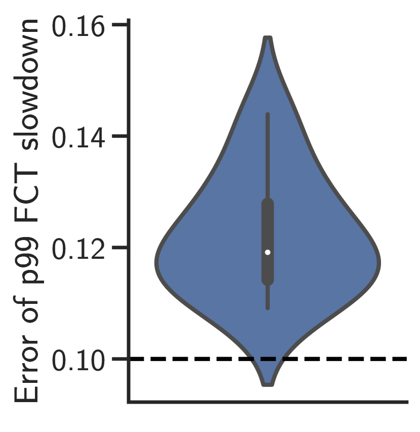
(a) p99 errors

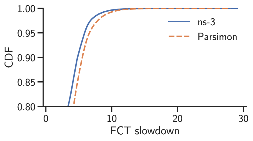
(b) CDF with the max p99 error (0.144)

Figure 12. Errors between ns-3 and Parsimon in estimated FCT slowdowns when there is a link failure. Fig. 12(a) shows the error distribution for p99 estimates from ten trials—each with one random link failure—with the dashed line showing the error with no link failure. Fig. 12(b) shows the CDF of FCT slowdowns for the trial with the highest p99 error. For the small oversubscribed topology used in this experiment, a link failure modestly increases estimation error.

One operational use case for Parsimon is to estimate counter-factual network performance in the presence of potential link failures or planned outages. In this section, we use the sample scenario from $\S$5.4 (matrix A, the Hadoop flow size distribution, low burstiness, 2-to-1 oversubscription, and a maximum link load of 68%) to evaluate Parsimon for this use case. For this configuration, the error in estimated p99 FCT slowdown between ns-3 and Parsimon was around 10%. Since link failures increase the load on the remaining links, we should expect some decreased accuracy for Parsimon in this case. On the other hand, simulating all possible network failures in ns-3 would be prohibitively expensive.

In selecting links to fail, we only consider links in ECMP groupings, such that the failure of one link causes traffic to be routed to the other links in the group. In Meta’s data center fabric [4], this corresponds to links between fabric switches and spine switches and links between ToR switches and fabric switches. In the small 32-rack topology used here ($\S$5.3 for details), there are 96 such links. We run ten trials, each time picking a random one of the links to fail, keeping the workload constant. We note that this setting represents a particularly bad case for Parsimon: in addition to the high link loads, the scenario uses an all-to-all communication pattern on a small and oversubscribed topology, which means each link failure in the core can have an outsized effect on other core links.

Fig. 12(a) shows the distribution of errors in p99 estimates. With a single link failure, the errors range from 11% to 14%, with a median error of 12%. Fig. 12(b) shows the estimated CDFs of FCT slowdown for the trial with the highest error.

Appendix C Studying Error Sources

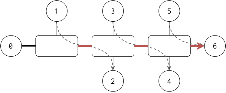
Figure 13. The parking lot topology used in $\S$C. In this topology, zero sends to six, one sends to two, three sends to four, and five sends to six. We refer to the traffic from zero to six as main traffic and to all other traffic as cross traffic. The bolded red links contain both main traffic and cross traffic, and we call them congested links.

Recall from $\S$3.6 that Parsimon’s approximations induce errors in its end-to-end estimates. In this appendix, we use microbenchmarks to study the effects of some pathological cases on Parsimon’s accuracy. For an initial discussion on these topics, please refer to $\S$3.6.

Throughout, we use the parking lot topology shown in Fig. 13 with 40 Gbps links. The flow of traffic through the topology is shown with arrows and described in the caption. We refer to the traffic from node zero to node six as main traffic and to all other traffic as cross traffic. The bolded red links contain both main traffic and cross traffic, and we call them congested links. In all experiments, we set the load of the main traffic to 25%. When there is cross traffic, its load is also 25%, yielding a total load of 50% on all three congested links. Lastly, to isolate the effects on the main path from zero to six, we measure FCT slowdown distributions only for the main traffic.

C.1. First-Hop Delays

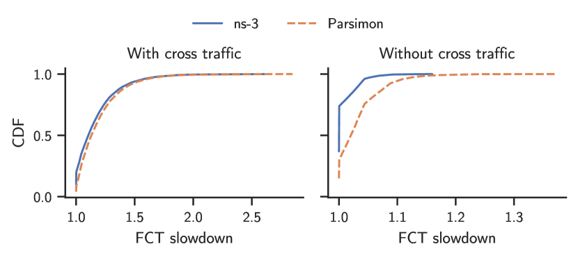
Figure 14. CDFs of FCT slowdown estimated by ns-3 and Parsimon for the main traffic, both with and without cross traffic. When there is cross traffic, errors arising from first-hop delays are second-order, as most delays are cause by queueing on the congested links. However, when there is no cross traffic, those errors become dominant. The graph on the right uses the same workload as the one on the left, except the cross traffic is removed. Note the different x-axes.

First, consider the case where all traffic in Fig. 13 originates from node zero and is destined to node six, and recall that all links have the same capacity. In a real network, all queueing in this scenario would occur at the first hop. Subsequent hops would see traffic completely smoothed, and they would therefore contributing zero queueing delay.

If we re-examine how link-level topologies are constructed in Fig. 4, we see that this smoothing effect is captured, since all traffic passes through edge links with the original edge-link capacities. However, for the link-level topologies in cases B and C of Fig. 4, it is possible for first-hop edge links to contribute delays that will be (erroniously) attributed to the target link. In most cases, we expect the magnitude of this error to be small. A target link will almost always have multiple sources, and only the traffic passing through the target link is simulated. Consequently, the first-hop delays in link-level simulation are expected to be small compared to delays accrued at target links.

The scenario which we first described—in which all traffic on a path originates from a single source—represents the worst case. Here, all target links (aside from the first hop) contribute no queueing delay, thus magnifying the error induced by repeatedly counting the first-hop delays for each target link. Fig. 14 shows this effect. In this experiment, the main traffic consists of one kilobyte flows, and the cross traffic consists of 10 kilobyte flows. All traffic follows a Poisson arrival process. With cross traffic, we see from the graph on the left that Parsimon accurately estimates the FCT slowdown distribution of the main traffic. However, when we remove the cross traffic, as done to produce the graph on the right, we see substantial error in Parsimon’s estimates due to the first-hop delays previously described. We note that this error exists even when there is cross traffic, but the error contributes so little to total delays—which are dominated by queueing at congested links—that Parsimon still maintains good accuracy.

C.2. Correlated and Simultaneous Delays

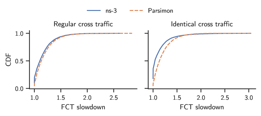
(a) Short flows (1 KB), Poisson cross traffic

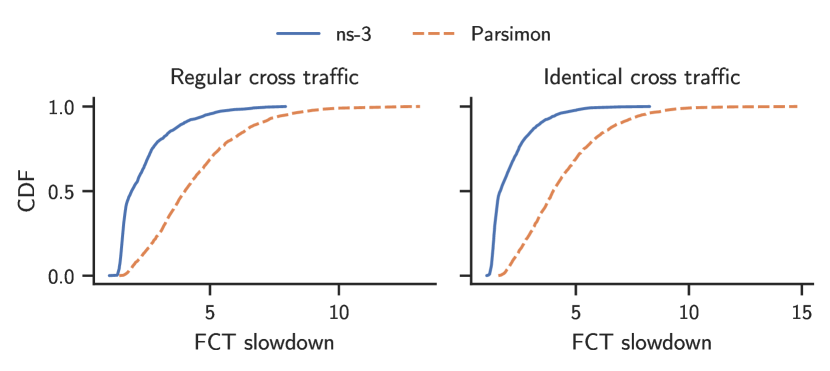
(b) Long flows (400 KB), Poisson cross traffic

Figure 15. CDFs of FCT slowdown estimated by ns-3 and Parsimon for the main traffic with regular or identical cross traffic. The main traffic consists either of short flows (Fig. 15(a)) or long flows (Fig. 15(b)). When delays are artifically correlated by replicating the same cross traffic across hosts, accuracy decreases for both short and long flows, with long flows seeing larger errors. In fact, long-flow estimates have significant error even when delays are not explicitly correlated; this is due to the simultaneous delays induced by the smooth Poisson cross traffic.

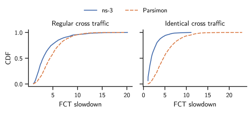
Figure 16. CDFs of FCT slowdown for the same scenario as in Fig. 15(b), but with bursty cross traffic (log-normal inter-arrival times, $\sigma=2$). When the cross traffic is bursty, long flows experience fewer simultaneous delays with regular cross traffic. This results in less error in Parsimon’s estimates.

Next we examine the effect of correlated and simultaneous delays on Parsimon’s accuracy. We begin by artificially correlating delays and examining the effect on estimated slowdown distributions. Note that if the delays along a path are positively correlated—for example, if the probability of encountering delay at hop $i+1$ is higher given there is delay at hop $i$—then we also expect to see more simultaneous delays along the path. We create these correlated delays by modulating the cross traffic. For regular unmodified cross traffic, we use the same setup as in the previous subsection ($\S$C.1). To artificially correlate delays, we replicate the exact sequence of flows from source one on sources three and five in Fig. 13, so that all three sources of cross traffic send the same flows at the same time. This produces an extreme case of correlation.

Because short-flow and long-flow estimates have different sources of error, we separate the two cases when generating the main traffic. For short flows we use the same one kilobyte flows as before, and for long flows we generate flows that are 10 times the maximum bandwidth-delay product, or 400 kilobytes. Fig. 15 shows the effect of correlating delays on Parsimon’s accuracy for short and long flows.

Short-flow main traffic.   In the case of short flows (Fig. 15(a)), a chief effect of increased correlation is to alter the probability that a flow will encounter queueing. For example, suppose a short flow traverses only two links at 50% utilization. If the delays of the two links are independent, we can estimate the probability that the flow encounters no delay (i.e., no queueing) as $50\%\times 50\%=25\%$. However, if the delays are perfectly positively correlated, then the probability that the flow encounters no delay increases to 50%. Parsimon does not capture this effect because it treats all links independently; in this experiment, this manifests as slight overestimates in FCT slowdown distributions.

Long-flow main traffic.   While the total delay for a short flow can be thought of as the sum of individual link delays, the same reasoning does not straightforwardly extend to long flows. Unlike a short flow, a long flow occupies multiple hops at the same time, and only the bottleneck at each instant contributes to end-to-end delay. Summing link delays is therefore only appropriate if different hops contribute significant delays at largely different times. However, Parsimon always aggregates individual link contributions by adding them, regardless of whether a link was the bottleneck when the delay was incurred. When we turn our attention to Fig. 15(b), we see that not only is the effect of identical cross traffic more severe, but also there is significant error even with regular cross traffic. This is because the cross traffic is smooth (recall that it uses uniform flow sizes and a Poisson arrival process). Smooth traffic results in small but frequent delays at congested links, increasing the chance that long flows will experience simultaneous delays.

In Fig. 16, we duplicate the scenario in Fig. 15(b), except we make the cross traffic bursty by using a log-normal inter-arrival time distribution with shape parameter $\sigma=2$. Because the cross traffic is bursty, there is less simultaneous delay in the regular case, and the induced error is less dominant. Consequently, Parsimon’s estimates are closer to the ground truth in the graph on the left. Identical cross traffic still induces large and frequent simultaneous delays, so the errors remain in the graph on the right.

Appendix D Clustering Details

Here we briefly describe the distance function and the thresholding critera we use in the evaluation ($\S$5) for clustering link-level simulations. First, recall from $\S$4.2 that the link features we extract are 1) the average load, 2) the flow size distribution, 3) the inter-arrival time distribution. For any two links, we compute distances between their features, and we cluster the links together if the distances are under some threshold.

Distance functions.   To compute a distance between link loads, we compute the error. If $a$ and $b$ are two link loads, error $e$ is computed as

$$e=\frac{|a-b|}{a}.$$

To compare distributions, there are many options. We opt for a function that is 1) easily interpretable, 2) scale-independent, and 3) adequately captures differences in the tail. To compute a distance between two distributions, we extract 1,000 percentiles from each of them, and we compute a weighted mean absolute percentage error (WMAPE) between them. Suppose $A$ and $B$ are the sequences of extracted percentiles. Then, WMAPE is computed as

$$\text{WMAPE}\ =\ \frac{\sum_{i=1}^{n}|A_{i}-B_{i}|}{\sum_{i=1}^{n}|A_{i}|}.$$

For our purpose, $A_{i}$ and $B_{i}$ are non-negative for all $i$. We note it is a bit counterintuitive for our distance functions not to commute. However, we have found that it is easy to set thresholds for these metrics, and they produce adequate clustering for the workloads under study.

Distance thresholds.   Recall that we only want to cluster two links together if we expect their simulation outputs to be similar. Consequently, when setting a threshold for link loads we must consider the network and the workload being assessed. At high load, small differences in link loads can yield large differences in the tails of FCT distributions; in these cases, we typically set tighter thresholds to preserve accuracy (as usual, this is subject to a speed-accuracy trade-off). For highly-loaded networks, we commonly require $e<0.001$ or $e<0.002$ for links to be clustered together. Ideally, this decision would be made on a link-by-link basis, so that tighter thresholds would be set only for high-load links—doing so may allow for more liberal clustering of the low-load links contributing little delay, resulting in more pruned simulations. However, the current prototype sets a single threshold per simulation. To set a threshold between distributions, we typically require $\text{WMAPE}<0.1$.

References

- [1] A. G. Alcoz, A. Dietmüller, and L. Vanbever. SP-PIFO: Approximating Push-In First-Out Behaviors using Strict-Priority Queues. In 17th USENIX Symposium on Networked Systems Design and Implementation (NSDI 20), pages 59–76, 2020.
- [2] M. Alizadeh, A. Greenberg, D. A. Maltz, J. Padhye, P. Patel, B. Prabhakar, S. Sengupta, and M. Sridharan. Data Center TCP (DCTCP). In Proceedings of the ACM SIGCOMM 2010 Conference, pages 63–74, 2010.
- [3] M. Alizadeh, A. Kabbani, T. Edsall, B. Prabhakar, A. Vahdat, and M. Yasuda. Less Is More: Trading a Little Bandwidth for Ultra-Low Latency in the Data Center. In 9th USENIX Symposium on Networked Systems Design and Implementation (NSDI 12), pages 253–266, 2012.
- [4] A. Andreyev. Introducing Data Center Fabric, the Next-Generation Facebook Data Center Network. https://engineering.fb.com/2014/11/14/production-engineering/introducing-data-center-fabric-the-next-generation-facebook-data-center-network/, 2014.
- [5] H. Balakrishnan, V. N. Padmanabhan, and R. H. Katz. The Effects of Asymmetry on TCP Performance. Mobile Networks and Applications, 4(3):219–241, 1999.
- [6] F. Baskett, K. M. Chandy, R. R. Muntz, and F. G. Palacios. Open, Closed, and Mixed Networks of Queues with Different Classes of Customers. Journal of the ACM (JACM), 22(2):248–260, 1975.
- [7] B. Burns, B. Grant, D. Oppenheimer, E. Brewer, and J. Wilkes. Borg, omega, and kubernetes. ACM Queue, 14:70–93, 2016.
- [8] M. Dalton, D. Schultz, J. Adriaens, A. Arefin, A. Gupta, B. Fahs, D. Rubinstein, E. C. Zermeno, E. Rubow, J. A. Docauer, et al. Andromeda: Performance, Isolation, and Velocity at Scale in Cloud Network Virtualization. In 15th USENIX Symposium on Networked Systems Design and Implementation (NSDI 18), pages 373–387, 2018.
- [9] A. Demers, S. Keshav, and S. Shenker. Analysis and Simulation of a Fair Queueing Algorithm. In Proceedings of the ACM SIGCOMM 1989 Conference, pages 514–528, 2020.
- [10] R. M. Fujimoto. Parallel Discrete Event Simulation. Communications of the ACM, 33(10):30–53, 1990.
- [11] P. Goyal, P. Shah, K. Zhao, G. Nikolaidis, M. Alizadeh, and T. E. Anderson. Backpressure Flow Control. In 19th USENIX Symposium on Networked Systems Design and Implementation (NSDI 22), pages 779–805, 2022.
- [12] J. R. Jackson. Networks of Waiting Lines. Operations Research, 5(4):518–521, 1957.
- [13] F. P. Kelly. Networks of Queues. Advances in Applied Probability, 8(2):416–432, 1976.
- [14] G. Kumar, N. Dukkipati, K. Jang, H. M. Wassel, X. Wu, B. Montazeri, Y. Wang, K. Springborn, C. Alfeld, M. Ryan, et al. Swift: Delay is Simple and Effective for Congestion Control in the Datacenter. In Proceedings of the ACM SIGCOMM 2020 Conference, pages 514–528, 2020.
- [15] J. Li, N. K. Sharma, D. R. K. Ports, and S. D. Gribble. Tales of the tail: Hardware, os, and application-level sources of tail latency. In Proceedings of the ACM Symposium on Cloud Computing, SOCC ’14, page 1–14, 2014.
- [16] Y. Li, R. Miao, H. H. Liu, Y. Zhuang, F. Feng, L. Tang, Z. Cao, M. Zhang, F. Kelly, M. Alizadeh, and M. Yu. HPCC: High Precision Congestion Control. In Proceedings of the ACM SIGCOMM 2019 Conference, page 44–58, 2019.
- [17] V. Liu, D. Halperin, A. Krishnamurthy, and T. Anderson. F10: A Fault-Tolerant Engineered Network. In 10th USENIX Symposium on Networked Systems Design and Implementation (NSDI 13), pages 399–412, 2013.
- [18] V. Misra, W.-B. Gong, and D. Towsley. Fluid-Based Analysis of a Network of AQM Routers Supporting TCP Flows with an Application to RED. In Proceedings of the ACM SIGCOMM 2000 Conference, pages 151–160, 2000.
- [19] R. Mittal, V. T. Lam, N. Dukkipati, E. Blem, H. Wassel, M. Ghobadi, A. Vahdat, Y. Wang, D. Wetherall, and D. Zats. TIMELY: RTT-Based Congestion Control for the Datacenter. In Proceedings of the ACM SIGCOMM 2015 Conference, page 537–550, 2015.
- [20] J. C. Mogul and J. Wilkes. Nines are Not Enough: Meaningful Metrics for Clouds. In Proceedings of the Workshop on Hot Topics in Operating Systems, pages 136–141, 2019.
- [21] B. Montazeri, Y. Li, M. Alizadeh, and J. Ousterhout. Homa: A Receiver-Driven Low-Latency Transport Protocol Using Network Priorities. In Proceedings of the ACM SIGCOMM 2018 Conference, pages 221–235, 2018.
- [22] D. Nicol and R. Fujimoto. Parallel Simulation Today. Annals of Operations Research, 53(1):249–285, 1994.
- [23] ns-3 Network Simulator. https://www.nsnam.org, 2020.
- [24] OpenSim. OMNeT++. https://www.omnetpp.org, 2018.
- [25] OPNET Network Simulator, 2015.
- [26] V. Paxson and S. Floyd. Why We Don’t Know How to Simulate the Internet. In Proceedings of the 1997 Winter Simulation Conference, pages 1037–1044, 1997.
- [27] K. Ramakrishnan and S. Floyd. A Proposal to Add Explicit Congestion Notification (ECN) to IP. Technical report, RFC 2481, January, 1999.
- [28] A. Roy, H. Zeng, J. Bagga, G. Porter, and A. C. Snoeren. Inside the Social Network’s (Datacenter) Network. In Proceedings of the ACM SIGCOMM 2015 Conference, pages 123–137, 2015.
- [29] A. Singh, J. Ong, A. Agarwal, G. Anderson, A. Armistead, R. Bannon, S. Boving, G. Desai, B. Felderman, P. Germano, A. Kanagala, J. Provost, J. Simmons, E. Tanda, J. Wanderer, U. Hölzle, S. Stuart, and A. Vahdat. Jupiter Rising: A Decade of Clos Topologies and Centralized Control in Google’s Datacenter Network. In Proceedings of the ACM SIGCOMM 2015 Conference, page 183–197, 2015.
- [30] B. K. Szymanski, A. Saifee, A. Sastry, Y. Liu, and K. Madnani. Genesis: A System for Large-scale Parallel Network Simulation. In Proceedings of the 16th Workshop on Parallel and Distributed Simulation (PADS), 2002.
- [31] R. Winter, R. Hernandez, G. Chawla, A. Faustini, C. Solder, T. Scheibe, D. Law, S. Ayandeh, B. Booth, B. Kohl, C. Lavacchia, S. Krishnamurthy, R. Karthikeyan, E. Multanen, and M. Wadekar. Ethernet Jumbo Frames. http://www.ethernetalliance.org/wp-content/uploads/2011/10/EA-Ethernet-Jumbo-Frames-v0-1.pdf, 2009.
- [32] Q. Yang, X. Peng, L. Chen, L. Liu, J. Zhang, H. Xu, B. Li, and G. Zhang. DeepQueueNet: Towards Scalable and Generalized Network Performance Estimation with Packet-Level Visibility. In Proceedings of the ACM SIGCOMM 2022 Conference, pages 441–457, 2022.
- [33] Q. Zhang, V. Liu, H. Zeng, and A. Krishnamurthy. High-Resolution Measurement of Data Center Microbursts. In Proceedings of the 2017 Internet Measurement Conference, pages 78–85, 11 2017.
- [34] Q. Zhang, K. K. Ng, C. Kazer, S. Yan, J. Sedoc, and V. Liu. MimicNet: Fast Performance Estimates for Data Center Networks with Machine Learning. In Proceedings of the ACM SIGCOMM 2021 Conference, pages 287–304, 2021.
- [35] S. Zhao, R. Wang, J. Zhou, J. Ong, J. C. Mogul, and A. Vahdat. Minimal Rewiring: Efficient Live Expansion for Clos Data Center Networks. In 16th USENIX Symposium on Networked Systems Design and Implementation (NSDI 19), pages 221–234, 2019.
- [36] Y. Zhu, H. Eran, D. Firestone, C. Guo, M. Lipshteyn, Y. Liron, J. Padhye, S. Raindel, M. H. Yahia, and M. Zhang. Congestion Control for Large-Scale RDMA Deployments. In Proceedings of the ACM SIGCOMM 2015 Conference, page 523–536, 2015.