Machine Learning Interatomic Potential for Simulations of Carbon at Extreme Conditions

Abstract

A Spectral Neighbor Analysis (SNAP) machine learning interatomic potential (MLIP) has been developed for simulations of carbon at extreme pressures (up to 5 TPa) and temperatures (up to 20,000 K). This was achieved using a large database of experimentally relevant quantum molecular dynamics (QMD) data, training the SNAP potential using a robust machine learning methodology, and performing extensive validation against QMD and experimental data. The resultant carbon MLIP demonstrates unprecedented accuracy and transferability in predicting the carbon phase diagram, melting curves of crystalline phases, and the shock Hugoniot, all within $3\,\mathrm{\%}$ of QMD. By achieving quantum accuracy and efficient implementation on leadership class high performance computing systems, SNAP advances frontiers of classical MD simulations by enabling atomic-scale insights at experimental time and length scales.

Carbon at extreme pressures and temperatures is a topic of great scientific interest for several disciplines including planetary science (Ross, 1981; Ancilotto et al., 1997; Benedetti et al., 1999; Kraus et al., 2017; Madhusudhan et al., 2012) and inertial confinement fusion (ICF) research (Ross et al., 2015; Millot et al., 2018; Hopkins et al., 2019; Kritcher et al., 2021). Methane ice at megabar pressures and temperatures of thousands of kelvins is predicted to convert to solid or liquid carbon in the cores of giant planets (Ancilotto et al., 1997; Benedetti et al., 1999; Kraus et al., 2017). A successful suppression of hydrodynamic instabilities seeded by solid and liquid carbon phases appearing upon strong compression of the outer diamond ablation shell of an ICF capsule (Casey et al., 2021) was the key for achieving a record-breaking, near-threshold fusion energy ignition at the National Ignition Facility (Tollefson, 2021).

The exploration of carbon’s behavior at extreme conditions is challenging for both theory and experiment. Shock and ramp compression experiments using powerful lasers (Duffy and Smith, 2019), pulsed power (Sinars et al., 2020) and bright X-ray sources (McMahon, 2020; Seddon et al., 2017) uncovered complicated mechanisms of inelastic deformations (Pavlovskii, 1971; Kondo and Ahrens, 1983; McWilliams et al., 2010; Lang et al., 2018; Katagiri et al., 2020; Winey et al., 2020), anomalous strength of diamond (McWilliams et al., 2010; Lang et al., 2018; Katagiri et al., 2020; Winey et al., 2020; MacDonald et al., 2020), unusual melting (Brygoo et al., 2007; Knudson et al., 2008; Eggert et al., 2010; Gregor et al., 2017; Millot et al., 2018, 2020) and liquid carbon properties (Knudson et al., 2008; Eggert et al., 2010), as well as extreme metastability of diamond well beyond the pressure-temperature range of its thermodynamic stability (Lazicki et al., 2021). Molecular dynamics (MD) simulations can provide a fundamental understanding of these phenomena, but to be of experimental relevance, it must accurately describe interatomic interactions in a system consisting of a large number of atoms.

Previous simulations of carbon at extreme conditions were predominantly performed using quantum molecular dynamics (QMD) based on density functional theory (DFT) (Scandolo et al., 1996; Grumbach and Martin, 1996; Wang et al., 2005; Correa et al., 2006, 2008; Knudson et al., 2008; Sun et al., 2009; Martinez-Canales et al., 2012; Benedict et al., 2014). Due to high computational cost, QMD simulations are limited to several hundred atoms for up to tens of picoseconds, which is insufficient for uncovering non-equilibrium processes at experimental time (ns) and length ($\mathrm{\mathrm{\mu}}m$) scales. In principle, these scales can be accessed by classical MD simulations on massively parallel computers (Thompson et al., 2022). However, empirical interatomic potentials developed for carbon at near ambient conditions (Brenner et al., 2002; Stuart et al., 2000; Los and Fasolino, 2003; Pastewka et al., 2008; Srinivasan et al., 2015) singularly fail upon extension to high pressures and temperatures (Oleynik et al., 2008; Perriot et al., 2013), thus compromising predictive power of atomistic simulations.

The advent of machine learning interatomic potentials (MLIPs) (Behler and Parrinello, 2007; Bartók et al., 2010) opens up exceptional opportunities for achieving a classical description of chemical bonding with quantum accuracy (Friederich et al., 2021). Although numerous MLIPs have been recently introduced and successfully applied to modeling properties of materials at ambient conditions (Behler and Parrinello, 2007; Bartók et al., 2010; Thompson et al., 2015; Wood and Thompson, 2018; Shapeev, 2015; Drautz, 2019; Zhang et al., 2018), including carbon (Khaliullin et al., 2010; Rowe et al., 2020), their exceptional power in describing diverse and complex atomic environments at megabar pressures and tens of thousand of kelvins has yet to be demonstrated.

This letter reports a significant advance in development of a quantum-accurate Spectral Neighbor Analysis Potential (SNAP) for simulations of carbon at extreme pressure-temperature (P-T) conditions. This includes construction of an experimentally relevant training database, implementation of a robust SNAP machine learning training methodology, and extensive validation against QMD and experimental data. The end result is the first MLIP that delivers unprecedented accuracy in simulating carbon over a remarkably wide range of pressures (from 0 to 50 Mbar) and temperatures (up to 20,000 K).

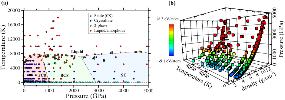
Figure 1: SNAP training database: a) pressure-temperature map of QMD and static DFT simulations included in the database, each represented by a P-T point on carbon phase diagram sampling FC8 (diamond), BC8, SC solid and liquid phases (total number of structures - $636$); b) pressure-temperature-density-energy/atom distribution.

In general, MLIPs fingerprint a unique local atomic environment around each atom by a set of descriptors. SNAP’s descriptors are bispectrum components $\{\mathbf{B^{\mathit{i}}}\}$ of the local neighbor density projected onto a basis of hyper-spherical harmonics in four dimensions (Thompson et al., 2015; Wood and Thompson, 2018). Other successful MLIPs – Neural Network Potentials (NNP) (Behler and Parrinello, 2007; Zhang et al., 2018), Gaussian Approximation Potential (GAP) (Bartók et al., 2010), the Moment Tensor Potential (MTP) (Shapeev, 2015) – employ mathematically different, but physically similar descriptors. All of them, including SNAP can be mapped into a general Atomic Cluster Expansion (ACE) descriptor framework (Drautz, 2019).

Herein, the total potential energy of the system of $N$ atoms is written as a sum of atomic energies $E^{i}$, which are quadratic functions of the bispectrum coefficients $\mathbf{B^{\mathit{i}}}$ (Wood and Thompson, 2018)

$$E_{tot}(\{\mathbf{r}^{N}\})=\sum_{i}E^{i};\qquad E^{i}=\mathbf{\boldsymbol{\boldsymbol{\beta}}\cdotp B^{\mathit{i}}+}\frac{1}{2}\mathbf{B^{\mathit{i}}\cdotp\boldsymbol{\alpha}\cdotp B^{\mathit{i}}}.$$ (1)

Machine-learning techniques are used to determine the symmetric matrix $\boldsymbol{\boldsymbol{\alpha}}$ and the vector $\boldsymbol{\boldsymbol{\beta}}$, the unknown parameters of SNAP, to reproduce potential energy, atomic forces and stress tensor for each structure in the DFT training database.

SNAP displays a good balance between computational cost and accuracy (Zuo et al., 2020). Both are controlled by SNAP hyperparameters – the cutoff radius $r_{cut}$ and the integer angular momentum $J$. The former specifies the number of neighbor atoms participating in the fingerprinting of atomic environment around each atom $i$ and the latter refers to the dimensionality of the descriptor space, i.e. the number of bispectrum descriptors$\{\mathbf{B^{\mathit{i}}}\}$: $(J+1)(J+3/2)(J+2)/2$ for each atom $\mathit{i}$.

The SNAP development includes: (i) construction of a robust training database of first-principles QMD data; (ii) machine-learning training; and (iii) extensive validation against QMD and experiment. These three tightly connected steps constitute a single development cycle. Several of such cycles are executed to improve upon deficiencies observed in previous iterations, see the development workflow in supplemental Fig. S2 (S_m, ). For example, during the validation, two-phase SNAP MD simulations produce melting lines of several high-pressure carbon phases in a substantial disagreement with QMD. The problem has been traced back to SNAP inaccuracies in calculation of enthalpies of solid and liquid phases along the melting line, which, according to Clausius–Clapeyron relation, define its slope $dT/dP$. Therefore, separate liquid and solid phases were added to the QMD training database to complement original combined two-phase solid-liquid structures. This update resulted in substantial improvements in SNAP accuracy upon execution of a new training cycle.

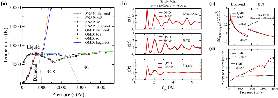
Figure 2: Validation of SNAP against QMD: (a) carbon phase diagram, including melting lines of diamond, BC8 and SC crystalline phases of carbon at pressures up to $5,000$ GPa and hydrostatic shock Hugoniot; (b) Radial distribution functions $g(r)$ for diamond, BC8 and liquid phase at diamond-bc8-liquid triple point ($840$ GPa, $7510$ K). (MD trajectories are averaged over $20$ ps time interval); c) density difference $\Delta\rho=\rho_{s}-\rho_{l}$ between solid (s) and liquid (l) phases (top panel) and average coordination number of carbon atoms (bottom panel) as a function of pressure along the melting lines of diamond and BC8. $\Delta\rho=0$ corresponds to melting line maxima: diamond – at $500\,\mathrm{GPa}$, BC8 – at $1,300\,\mathrm{GPa}$.

One of the highlights of our MLIP development is the dedicated construction of a SNAP training database of experimentally relevant QMD of large systems (by QMD standards) – up to 1,024 atoms. These are individual frames (1-3 frames per simulation) from QMD production simulations of physical properties of carbon (melting lines, hydrostatic and uniaxial isotherms, shock Hugoniot) performed within a wide range of pressures (from $0$ to $5$ TPa), temperatures (from $0$ to $40,000$ K) and densities (from $2.9$ to $13.6$ $\mathrm{g/cm^{3}}$). For example, MD frames for each $(P,T)$ point along the melting lines of several crystalline carbon phases were taken from production two-phase QMD simulation (Belonoshko, 1994). These complex cells contain both liquid and solid parts separated by a realistic solid-liquid interface, which add an additional complexity to the SNAP database. A series of complimentary QMD simulations of liquid and solid phases were also included in the database. The QMD data is supplemented by static DFT calculations of binding energy curves, point and extended defects, and metastable carbon structures obtained from dedicated crystal structure searching (Williams et al., 2022). Fig. 1 displays the range of pressures, temperatures and energies covered by QMD simulations. The SNAP database, consisting of $636$ structures, samples 124,907 unique atomic environments. Each structure of $N$ atoms contributes $1$ total energy, $6$ stress components and $3N$ atomic forces resulting in a total training complexity (the number of regression equations to fit) of $388,077$. Additional information on database composition and its generation is provided in the Supplemental Material (S_m, ).

Once the database is constructed, the SNAP model for the total potential energy, stress tensor components and atomic forces is trained using machine learning techniques to determine SNAP parameters $\boldsymbol{\alpha}$ and $\boldsymbol{\beta}$ through minimization of an objective function - a sum of the normalized squared differences between DFT and SNAP energies, stresses and atomic forces (Fig. S2) (S_m, ). The training is performed in a series of iterations. For a given set of weights, the SNAP parameters $\boldsymbol{\boldsymbol{\alpha}}$ and $\boldsymbol{\beta}$ are determined through weighted linear regression as implemented in FitSNAP package (fit, ). The weights are then optimized to minimize the objective function using a genetic algorithm (GA) within DAKOTA software package (Adams, 2021). At every step of GA minimization FitSNAP is called with the current set of weights to determine new $\boldsymbol{\boldsymbol{\alpha}}$ and $\mathbf{\boldsymbol{\beta}}$, which are then fed back to update the objective function being minimized (Fig. S2) (S_m, ). The iterations stop when the GA minimization converges to a final set of weights. In addition to group weights, the SNAP hyperparameters, $r_{cut}$ and $J$ are optimized in an offset fashion to find a right balance between SNAP accuracy and computational efficiency (Fig. S2 (S_m, )). The final values for the SNAP hyperparameters are $r_{cut}=2.7\,\mathrm{\text{\r{A}}}$ and $J=4$. The resultant quality of SNAP training is discussed in Supplemental Material (S_m, ).

The critical part of SNAP potential development is a thorough validation of SNAP MD results against QMD and experimental data. Only one to three QMD frames per (P,T) state were included in the SNAP training database. Therefore, simulating these states with SNAP using much larger simulations cells and performing thermodynamic averaging of atomic trajectories containing tens of thousands of frames to obtain stresses, densities, internal energies, as well as radial distribution functions is considered as a rigorous validation test against QMD. Further, these validation simulations are extended to sample a variety of pressures and temperatures not included in the database and compared to both QMD and experiment to demonstrate SNAP transferability.

The important validation test is concerned with carbon phase diagram, including melting lines of several high-pressure phases at pressures up to $5,000$ GPa, see Fig. (2a). A series of isobaric-isothermal NPT two-phase MD simulations were run at a given pressure but varying temperature to determine the P-T value of the phase coexistence (Belonoshko, 1994). SNAP melting lines are in excellent agreement with those from QMD, the average temperature error being $\sim 200\,\mathrm{K}$ or $3\%$ in a pressure interval from $0$ to $5,000$ GPa. Fig. 2(b) displays SNAP and QMD radial distribution functions $g(r)$ at diamond-BC8-liquid triple point: they are almost indistinguishable from each other.

A remarkable property of carbon at extreme conditions is the negative slope ($dT/dP$) of diamond and BC8 melting lines at high pressures (Grumbach and Martin, 1996; Wang et al., 2005; Correa et al., 2006, 2008; Benedict et al., 2014; Eggert et al., 2010). This is because liquid carbon becomes denser than the corresponding solid phase upon increase of pressure above $\sim 500$ GPa for diamond and $\sim 1,300$ GPa for BC8, see Fig. 2(c). This can be traced back to a significant increase of carbon packing in the liquid as carbon atom coordination changes from less than 4 to higher values, see Fig. 2(d). SNAP accurately predicts this subtle change in density upon increase of pressure as well as corresponding pressure-dependent evolution of the average coordination of carbon atoms ( Fig. 2(d)), which is in an excellent agreement with QMD. The latter is a result of “snap-on” agreement between QMD and SNAP radial distribution functions for both diamond and BC8 over a large range of pressures (Fig. S4 (S_m, )).

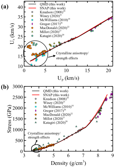
Figure 3: Carbon shock Hugoniot calculated by QMD and SNAP and compared with experimental data. (a) $U_{s}-U_{p}$ Hugoniot (b) pressure-density Hugoniots. Points correspond to experimental data.

Another validation test of great experimental importance is the prediction of the carbon shock Hugoniot, which passes through both solid and liquid parts of the phase diagram (Fig. 2(a)). The Hugoniot points are calculated in a hydrodynamic approximation by ignoring crystalline anisotropy in a series of MD simulations at a given pressure $P$ but varying temperature $T$ to satisfy the Hugoniot condition of conservation of mass, momentum, and energy: $\frac{1}{2}(P+P_{0})(V-V_{0})=(E-E_{0})$, where $P$, $V,$ and $E$ are the pressure, volume, and internal energy at a given point on the Hugoniot, and $P_{0}$, $V_{0}$, and $E_{0}$ are those at ambient conditions of $0$ GPa and $300$ K. The Hugoniot in $(P,T)$ space is shown in Fig. 2(a), in pressure-density $(P-\rho)$ space – in Fig. 3(b) and particle velocity $U_{p}$ – shock velocity $U_{s}$ space – in Fig. 3(a). The SNAP Hugoniots (red lines in Figs 2(a) and 3) are in a very good agreement with those from QMD (black lines in Figs 2(a) and 3). Visible differences in temperature of the P–T Hugoniot at very high temperatures (Fig. 2(a)) are due to electronic entropy effects, which are not captured by any classical interatomic potential.

Both SNAP and QMD Hugoniots are also in a very good agreement with multiple experiments in a pressure range from $300$ to $1,500\,\mathrm{GPa}$ (Knudson et al., 2008; McWilliams et al., 2010; Gregor et al., 2017; MacDonald et al., 2020; Millot et al., 2020; Winey et al., 2020; Katagiri et al., 2020). Some difference between SNAP/QMD and experiment at higher pressures is due to experimental uncertainty in density, which is not measured directly, but rather determined using an impedance matching method (Gregor et al., 2017; Millot et al., 2020). Differences at low pressures between experiment (McWilliams et al., 2010; MacDonald et al., 2020; Winey et al., 2020) and SNAP/QMD (Fig. 3(a)) are due to crystalline anisotropy and strength effects, which are not well described by a hydrodynamic approximation (Winey et al., 2020). To make a proper comparison with experiment in this split elastic-inelastic shock wave regime, explicit large-scale SNAP MD simulations of piston-driven shock waves are required, which will be the focus of future work.

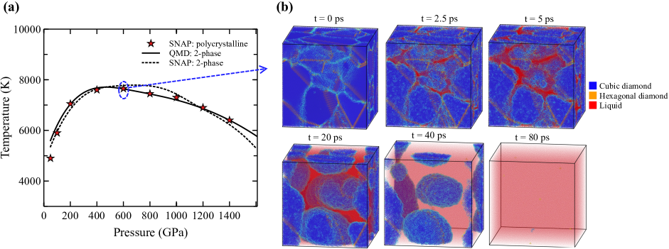
Figure 4: (a) Comparison of diamond melting curves calculated by three methods: QMD 2-phase (solid line), SNAP 2-phase (dashed line), and direct melting of 1 million atom polycrystalline sample using SNAP (stars); (b) Time progression of polycrystalline sample melting at $600$ GPa and $7750$ K. The sample is initially composed of crystalline diamond regions (blue) separated by grain boundaries (light blue). Liquid regions (red) emerge at the grain boundaries, grow in size, and eventually consume the isolated diamond crystallites.

To demonstrate SNAP’s ability to attack problems that are impossible to solve with QMD, we simulated melting of polycrystalline diamond at pressures between 50 and 1,200 GPa using a 1 million atom sample (Fig. 4). For each pressure point, a series of NPT simulations is performed to determine the temperature at the onset of melting. In addition to validating SNAP, this simulation also validates the two-phase melting curve calculation. The presence of grain boundaries suppresses superheating characteristic of single crystals: the melting starts at the most weakly bonded defective regions of the sample, followed by the growth of liquid fraction at the expense of crystalline grains, which gradually transform to shrinking round crystallites embedded in the liquid carbon (Fig. 4).

This work represents a major step towards solving extremely challenging but fundamentally important problem of predictive atomic-scale simulations of carbon at extreme pressure-temperature conditions at experimental time and length scales. The quantum-accurate SNAP is the first MLIP that describes the properties of carbon at extreme pressures up to $5$ TPa and temperatures up to $20,000$ K, including the phase diagram, melting curves of diamond, BC8 and simple cubic phases of carbon and shock Hugoniots with unprecedented accuracy within $3\,\mathrm{\%}$ of QMD results. SNAP’s linear scaling with number of atoms, and its efficient implementation within the LAMMPS MD simulation package (Thompson et al., 2022) allows billion atom simulations on leadership class high performance computing systems (Nguyen-Cong et al., 2021). By advancing frontiers of classical MD simulations, SNAP enables new insights by uncovering fundamental atomic-scale mechanisms of materials response which are difficult or even impossible to observe in experiment.

The work at USF is supported by DOE/NNSA (grant DE-NA- 0003910). The work at KTH is supported by Swedish Scientific Council (VR) (grant 2017-03744). Sandia National Laboratories is a multi-mission laboratory managed and operated by National Technology and Engineering Solutions of Sandia, LLC, a wholly owned subsidiary of Honeywell International, Inc., for the U.S. Department of Energy’s (DOE) National Nuclear Security Administration under Contract No. DE-NA0003525. The computations were performed using leadership-class HPC systems: OLCF Summit at Oak Ridge National Laboratory (ALCC and INCITE awards MAT198) and TACC Frontera at University of Texas at Austin (LRAC award DMR21006).

References

- Ross (1981) M. Ross, Nature 292, 435 (1981).
- Ancilotto et al. (1997) F. Ancilotto, G. L. Chiarotti, S. Scandolo, and E. Tosatti, Science 275, 1288 (1997).
- Benedetti et al. (1999) L. R. Benedetti, J. H. Nguyen, W. A. Caldwell, H. Liu, M. Kruger, and R. Jeanloz, Science 286 (1999).
- Kraus et al. (2017) D. Kraus, J. Vorberger, A. Pak, N. J. Hartley, et al., Nat. Astron. 1, 606 (2017).
- Madhusudhan et al. (2012) N. Madhusudhan, K. K. M. Lee, and O. Mousis, Astrophys. J. 759, L40 (2012).
- Ross et al. (2015) J. S. Ross, D. Ho, J. Milovich, T. Döppner, J. McNaney, et al., Phys. Rev. E 91, 1 (2015).
- Millot et al. (2018) M. Millot, P. M. Celliers, P. A. Sterne, L. X. Benedict, A. A. Correa, S. Hamel, S. J. Ali, et al., Phys. Rev. B 97, 144108 (2018).
- Hopkins et al. (2019) L. B. Hopkins, S. LePape, L. Divol, A. Pak, E. Dewald, et al., Plasma Phys. Control. Fusion 61, 014023 (2019).
- Kritcher et al. (2021) A. L. Kritcher, A. B. Zylstra, D. A. Callahan, O. A. Hurricane, et al., Phys. Plasmas 28, 072706 (2021).
- Casey et al. (2021) D. T. Casey, B. J. MacGowan, J. D. Sater, A. B. Zylstra, O. L. Landen, J. Milovich, O. A. Hurricane, A. L. Kritcher, et al., Phys. Rev. Lett. 126, 25002 (2021).
- Tollefson (2021) J. Tollefson, Nature 597, 163 (2021).
- Duffy and Smith (2019) T. S. Duffy and R. F. Smith, Front. Earth Sci. 7, 1 (2019).
- Sinars et al. (2020) D. B. Sinars, M. A. Sweeney, C. S. Alexander, D. J. Ampleford, T. Ao, et al., Phys. Plasmas 27, 070501 (2020).
- McMahon (2020) M. I. McMahon, in Synchrotron Light Sources Free. Lasers, edited by E. J. Jaeschke, S. Khan, J. R. Schneider, and J. B. Hastings (Springer International Publishing, 2020) pp. 1857–1896.
- Seddon et al. (2017) E. A. Seddon, J. A. Clarke, D. J. Dunning, C. Masciovecchio, C. J. Milne, F. Parmigiani, D. Rugg, J. C. H. Spence, N. R. Thompson, K. Ueda, S. M. Vinko, J. S. Wark, and W. Wurth, Reports Prog. Phys. 80, 115901 (2017).
- Pavlovskii (1971) M. N. Pavlovskii, Sov. Phys. - Solid State 13, 741 (1971).
- Kondo and Ahrens (1983) K.-I. Kondo and T. J. Ahrens, Geophys. Res. Lett. 10, 281 (1983).
- McWilliams et al. (2010) R. S. McWilliams, J. H. Eggert, D. G. Hicks, D. K. Bradley, P. M. Celliers, D. K. Spaulding, T. R. Boehly, G. W. Collins, and R. Jeanloz, Phys. Rev. B 81, 27 (2010).
- Lang et al. (2018) J. M. Lang, J. M. Winey, and Y. M. Gupta, Phys. Rev. B 97, 104106 (2018).
- Katagiri et al. (2020) K. Katagiri, N. Ozaki, Y. Umeda, T. Irifune, N. Kamimura, K. Miyanishi, T. Sano, T. Sekine, and R. Kodama, Phys. Rev. Lett. 125, 185701 (2020).
- Winey et al. (2020) J. M. Winey, M. D. Knudson, and Y. M. Gupta, Phys. Rev. B 101, 184105 (2020).
- MacDonald et al. (2020) M. J. MacDonald, E. E. McBride, E. Galtier, M. Gauthier, E. Granados, D. Kraus, A. Krygier, A. L. Levitan, A. J. MacKinnon, I. Nam, W. Schumaker, P. Sun, T. B. van Driel, J. Vorberger, Z. Xing, R. P. Drake, S. H. Glenzer, and L. B. Fletcher, Appl. Phys. Lett. 116, 234104 (2020).
- Brygoo et al. (2007) S. Brygoo, E. Henry, P. Loubeyre, J. Eggert, M. Koenig, B. Loupias, A. Benuzzi-Mounaix, and M. Rabec Le Gloahec, Nat. Mater. 6, 274 (2007).
- Knudson et al. (2008) M. D. Knudson, M. P. Desjarlais, and D. H. Dolan, Science 322, 1822 (2008).
- Eggert et al. (2010) J. H. Eggert, D. G. Hicks, P. M. Celliers, D. K. Bradley, R. S. McWilliams, R. Jeanloz, J. E. Miller, T. R. Boehly, and G. W. Collins, Nat. Phys. 6, 40 (2010).
- Gregor et al. (2017) M. C. Gregor, D. E. Fratanduono, C. A. McCoy, D. N. Polsin, A. Sorce, J. R. Rygg, G. W. Collins, T. Braun, P. M. Celliers, J. H. Eggert, D. D. Meyerhofer, and T. R. Boehly, Phys. Rev. B 95, 144114 (2017).
- Millot et al. (2020) M. Millot, P. A. Sterne, J. H. Eggert, S. Hamel, M. C. Marshall, and P. M. Celliers, Phys. Plasmas 27, 102711 (2020).
- Lazicki et al. (2021) A. Lazicki, D. McGonegle, J. R. Rygg, D. G. Braun, D. C. Swift, et al., Nature 589, 532 (2021).
- Scandolo et al. (1996) S. Scandolo, G. Chiarotti, and E. Tosatti, Phys. Rev. B 53, 5051 (1996).
- Grumbach and Martin (1996) M. P. Grumbach and R. M. Martin, Phys. Rev. B 54, 15730 (1996).
- Wang et al. (2005) X. Wang, S. Scandolo, and R. Car, Phys. Rev. Lett. 95, 1 (2005).
- Correa et al. (2006) A. A. Correa, S. A. Bonev, and G. Galli, Proc. Natl. Acad. Sci. U. S. A. 103, 1204 (2006).
- Correa et al. (2008) A. Correa, L. Benedict, D. Young, E. Schwegler, and S. A. Bonev, Phys. Rev. B 78, 25 (2008).
- Sun et al. (2009) J. Sun, D. D. Klug, and R. Marton̂ák, J. Chem. Phys. 130, 194512 (2009).
- Martinez-Canales et al. (2012) M. Martinez-Canales, C. J. Pickard, and R. J. Needs, Phys. Rev. Lett. 108, 45704 (2012).
- Benedict et al. (2014) L. X. Benedict, K. P. Driver, S. Hamel, B. Militzer, T. Qi, A. A. Correa, A. Saul, and E. Schwegler, Phys. Rev. B 89, 224109 (2014).
- Thompson et al. (2022) A. P. Thompson, H. M. Aktulga, R. Berger, D. S. Bolintineanu, W. M. Brown, P. S. Crozier, P. J. in ’t Veld, A. Kohlmeyer, S. G. Moore, T. D. Nguyen, R. Shan, M. J. Stevens, J. Tranchida, C. Trott, and S. J. Plimpton, Comput. Phys. Commun. 271, 108171 (2022).
- Brenner et al. (2002) D. W. Brenner, O. A. Shenderova, J. A. Harrison, S. J. Stuart, B. Ni, and S. B. Sinnott, J. Phys. Condens. Matter 14, 783 (2002).
- Stuart et al. (2000) S. J. Stuart, A. B. Tutein, and J. A. Harrison, J. Chem. Phys 112, 6472 (2000).
- Los and Fasolino (2003) J. H. Los and A. Fasolino, Phys. Rev. B 68, 024107 (2003).
- Pastewka et al. (2008) L. Pastewka, P. Pou, R. Pérez, P. Gumbsch, and M. Moseler, Phys. Rev. B 78, 161402 (2008).
- Srinivasan et al. (2015) S. G. Srinivasan, A. C. T. van Duin, and P. Ganesh, J. Phys. Chem. A 119, 571 (2015).
- Oleynik et al. (2008) I. I. Oleynik, A. C. Landerville, S. V. Zybin, M. L. Elert, and C. T. White, Phys. Rev. B 78, 180101 (2008).
- Perriot et al. (2013) R. Perriot, X. Gu, Y. Lin, V. V. Zhakhovsky, and I. I. Oleynik, Phys. Rev. B 88, 064101 (2013).
- Behler and Parrinello (2007) J. Behler and M. Parrinello, Phys. Rev. Lett. 98, 1 (2007).
- Bartók et al. (2010) A. P. Bartók, M. C. Payne, R. Kondor, and G. Csányi, Phys. Rev. Lett. 104, 136403 (2010).
- Friederich et al. (2021) P. Friederich, F. Häse, J. Proppe, and A. Aspuru-Guzik, Nat. Mater. 20, 750 (2021).
- Thompson et al. (2015) A. P. Thompson, L. P. Swiler, C. R. Trott, S. M. Foiles, and G. J. Tucker, J. Comput. Phys. 285, 316 (2015).
- Wood and Thompson (2018) M. A. Wood and A. P. Thompson, J. Chem. Phys. 148, 241721 (2018).
- Shapeev (2015) A. V. Shapeev, Multiscale Model. Simul. 14, 1 (2015).
- Drautz (2019) R. Drautz, Phys. Rev. B 99, 1 (2019).
- Zhang et al. (2018) L. Zhang, J. Han, H. Wang, R. Car, and E. Weinan, Phys. Rev. Lett. 120, 143001 (2018).
- Khaliullin et al. (2010) R. Z. Khaliullin, H. Eshet, T. D. Kühne, J. Behler, and M. Parrinello, Phys. Rev. B 81, 18 (2010).
- Rowe et al. (2020) P. Rowe, V. L. Deringer, P. Gasparotto, G. Csányi, and A. Michaelides, J. Chem. Phys. 153, 034702 (2020).
- Zuo et al. (2020) Y. Zuo, C. Chen, X. Li, Z. Deng, Y. Chen, J. Behler, G. Csányi, A. V. Shapeev, A. P. Thompson, M. A. Wood, and S. P. Ong, J. Phys. Chem. A 124, 731 (2020).
- (56) See Supplemental Material at http://link.aps.org/ supplemental/ for details on (1) SNAP training database; (2) SNAP machine learning development workflow; (3) Accuracy assessment of SNAP training; (4) SNAP validation: Radial Distribution Functions of solid and liquid phases along diamond and BC8 melting lines.
- Belonoshko (1994) A. B. Belonoshko, Geochimica et Cosmochimica Acta 58, 4039 (1994).
- Williams et al. (2022) A. S. Williams, K. Nguyen-Cong, J. T. Willman, and I. I. Oleynik, Phys. Chem. Lett. , submitted for publication (2022).
- (59) FitSNAP: Software for generating SNAP machine learning interatomic potentials: http://github.com/FitSNAP.
- Adams (2021) B. Adams, Dakota, A Multilevel Parallel Object-Oriented Framework for Design Optimization, Parameter Estimation, Uncertainty Quantification, and Sensitivity Analysis: Version 6.14 User’s Manual (2021).
- Nguyen-Cong et al. (2021) K. Nguyen-Cong, J. T. Willman, S. G. Moore, A. B. Belonoshko, R. Gayatri, E. Weinberg, M. A. Wood, A. P. Thompson, and I. I. Oleynik, Proc. Int. Conf. High Perform. Comput. Networking, Storage Anal. , 1 (2021).