An Interferometric View of H-MM1. I. Direct Observation of NH3 Depletion

Abstract

Spectral lines of ammonia, NH3, are useful probes of the physical conditions in dense molecular cloud cores. In addition to advantages in spectroscopy, ammonia has also been suggested to be resistant to freezing onto grain surfaces, which should make it a superior tool for studying the interior parts of cold, dense cores. Here we present high-resolution NH3 observations with the Very Large Array (VLA) and Green Bank Telescope (GBT) towards a prestellar core. These observations show an outer region with a fractional NH3 abundance of $X(\ce{NH3})=(1.975\pm 0.005)\times 10^{-8}$ ($\pm$10% systematic), but it also reveals that after all, the $X(\ce{NH3})$ starts to decrease above a $\ce{H2}$ column density of $\approx 2.6\times 10^{22}\,\rm cm^{-2}$. We derive a density model for the core and find that the break-point in the fractional abundance occurs at the density $n(\ce{H2})\sim 2\times 10^{5}\,\rm cm^{-3}$, and beyond this point the fractional abundance decreases with increasing density, following the power law $n^{-1.1}$. This power-law behavior is well reproduced by chemical models where adsorption onto grains dominates the removal of ammonia and related species from the gas at high densities. We suggest that the break-point density changes from core to core depending on the temperature and the grain properties, but that the depletion power law is anyway likely to be close to $n^{-1}$ owing to the dominance of accretion in the central parts of starless cores.

1 Introduction

Dense cores are the places where stars are formed. Their physical conditions determine when the gravitational collapse starts and how it proceeds (di Francesco et al., 2007). Observations of molecular lines allow us to extract information not only about the physical structure of dense cores but also about their chemical composition (Bergin & Tafalla, 2007).

When high densities and low temperatures are present, gas-phase molecules can be depleted because of accretion onto the dust grains. The effect of depletion is commonly observed in CO (and isotopologues), and it is identified as a strong decrease in the CO abundance towards the central part of a dense core (e.g., Caselli et al., 1999; Tafalla et al., 2004). Surprisingly, some nitrogen-bearing species, such as NH3, N2H+ and CN, do not present strong evidence for depletion (Tafalla et al., 2004; Crapsi et al., 2007; Hily-Blant et al., 2008, 2010). However, it is theoretically expected that all species, other than pure hydrogen species and helium, should be depleted by at least two orders of magnitude in the central region of a dense, starless core; this region can be called the zone of “complete depletion” (Walmsley et al., 2004). In the past, modeling of single dish observations have provided indirect evidence for depletion of N2H+ in the L183 and L1544 dense cores (Pagani et al., 2005, 2007; Redaelli et al., 2019). Only recent observations with ALMA, resolving the densest parts of the prestellar core L1544, show evidence for depletion of deuterated ammonia, NH2D (Caselli et al., 2022).

To validate the concept of complete depletion, it is important to investigate if also the common isotopolog of ammonia, NH3, is also depleted at high densities. The starless core H-MM1 (Johnstone et al., 2004; Parise et al., 2011) is an excellent target for this purpose. H-MM1 lies in relative isolation on the outskirts of the L1688 region in the nearby Ophiuchus molecular cloud. The distance to L1688 is $\approx$138.4$\pm$2.6 pc (Ortiz-León et al., 2018). Ammonia line emission in the L1688 region has been previously studied with single-dish observations (Friesen et al., 2017; Harju et al., 2017; Chen et al., 2019; Auddy et al., 2019; Choudhury et al., 2020, 2021). These studies show a clear transition from the supersonic turbulence to a subsonic regime at the boundary of the H-MM1 core, and that the interior parts of the core are characterized by a high degree of deuteration in NH3 (Harju et al., 2017). This suggests that the densities and temperatures in the central region are appropriate for NH3 depletion.

High-resolution NH3 observations are also useful for the interpretation of recent ALMA observations that revealed the presence of a methanol ($\rm CH_{3}OH$) sheath around the dense core (Harju et al., 2020). Of the methanol desorption mechanisms discussed in Harju et al. (2020), shocks and grain-grain collisions induced by vigorous turbulence or shear instability should be associated with increased kinetic temperatures or velocity dispersion in the methanol emission region. Ammonia provides excellent means to determine these quantities and thereby test these desorption scenarios.

Here we present NH3 (1,1) and (2,2) observations of the starless core H-MM1 with the Karl G. Jansky Very Large Array (VLA), which we combine with previous Robert C. Byrd Green Bank Telescope (GBT) observations (Friesen et al., 2017). The acquired data allow us to study the NH3 emission at high angular resolution to resolve the possible NH3 depletion zone and to improve our knowledge of the origin of methanol.

2 Data

2.1 VLA

We conducted VLA observations of H-MM1 on 2020 January 9, 12, 14, and 18 in the D-array configuration (project 19B-178, PI: Pineda). We used the high-frequency K-band receiver and configured the WIDAR correlator to observe the NH3 (1,1) and (2,2) lines with 8 and 4 MHz bandwidth windows, respectively. Each window has a channel separation of 5.208 kHz ($\approx$0.065 $\rm km\,s^{-1}$). The quasar 3C 286 is used as the flux calibrator, J1256-0547 as the bandpass calibrator, and J1625-2527 as the phase calibrator.

The calibration was performed using the VLA pipeline with the Common Astronomy Software Applications package (CASA) version 5.6.2-2 (McMullin et al., 2007). This included Hanning-smoothing, and therefore the effective spectral resolution is 0.13 $\rm km\,s^{-1}$. The imaging used the tclean command with natural weighting and uvtaper to increase the signal to noise ratio, a restoring beam of 6″, and with multi-scale clean (with scales 0, 6, 18, and 54″and a smallscalebias parameter of 0). We also included the NH3 single dish data obtained with the Robert C. Byrd Green Bank Telescope (Friesen et al., 2017) as a model image to recover the extended emission using the startmodel option in tclean. This method initializes the clean model image as the single dish data. The final noise level achieved in the data cubes is 3.5 m$\rm Jy\,beam^{-1}$ per channel, which corresponds to $\approx$0.21 K per channel. We estimate our absolute calibration uncertainty to be 10%.

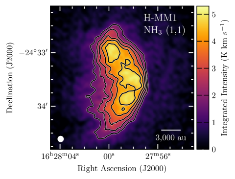
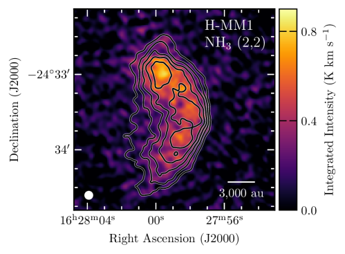
Figure 1: Integrated intensity maps of the NH3 (1,1) and (2,2) main line components are shown in the left and right panels, respectively. The contours are for NH3 (1,1) in both panels. The contour levels start from 1.5 $\rm K\,km\,s^{-1}$ and the spacing is 0.75 $\rm K\,km\,s^{-1}$. The beam size and the scale bar are shown at bottom left and right, respectively.

The integrated intensity maps of the main hyperfine component of the NH3 (1,1) and (2,2) lines are shown in Fig. 1.

2.2 Total H2 Column Density

The H-MM1 core appears as an absorption feature in the 8 $\rm\mu m$ map measured by the InfraRed Array Camera (IRAC) of the Spitzer Space Telescope. We use this to derive a high-resolution $\ce{H2}$ column density map of the core. The method is described in Appendix A of Harju et al. (2020), and briefly summarized here. The method also uses the 850 $\rm\mu m$ emission map from SCUBA-2 (Pattle et al., 2015), and the dust color temperature map, $T_{\rm C}$, derived from Herschel/SPIRE maps (Harju et al., 2017). We assume the dust opacity model for unprocessed dust grains with thin ice mantles by Ossenkopf & Henning (1994). This model has a dust emissivity index of $\beta=2.0$ over Herschel/SPIRE wavelengths (250–500 $\rm\mu m$). The absorption cross-sections per unit mass of gas at 8 $\rm\mu m$ and 850 $\rm\mu m$ are $\kappa_{8\,\rm\mu m}=8.86\,\rm cm^{2}\,\rm g^{-1}$ and $\kappa_{850\,\rm\mu m}=1.13\times 10^{-2}\,\rm cm^{2}\,\rm g^{-1}$, respectively. The Spitzer map is smoothed to the resolution of the VLA ammonia map, $6\,\arcsec$, before the derivation of the column density map. The resulting $N(\ce{H2})$ distribution is shown in Fig. 2.

Lefèvre et al. (2016) pointed out that scattering by dust particles may bias column density derived from $8\,\rm\mu m$ absorption. This issue is discussed in Appendix A. Simulations using different dust models show that the effect of scattering is likely to be small compared to the uncertainties related to the intensities of the foreground and background emission components, and thermal dust emission at 8 $\rm\mu m$. The 8 $\rm\mu m$ background intensity in the region of H-MM1 is $\sim$10 $\rm MJy\,sr^{-1}$, whereas the scattered intensity according to our simulations should stay below $0.1\,\rm MJy\,sr^{-1}$ (see Appendix A).

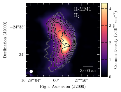
Figure 2: Dust derived total H2 column density map of the H-MM1 region. The map shows a peak close to the center of the image. The resolution and scale bar are shown at bottom left and right, respectively. The contours show the NH3 (1,1) integrated intensity, as in Fig 1.

3 Observational Results

3.1 Line Fits

We simultaneously fit the NH3 (1,1) and (2,2) line profiles with pyspeckit using the cold-ammonia model (Friesen et al., 2017), which gives a centroid velocity, $V_{\rm LSR}$, velocity dispersion, $\sigma_{\rm v}$, kinetic temperature, $T_{\rm k}$, excitation temperature, $T_{\rm ex}$, and total column density of NH3, $N(\ce{NH3})$, with an assumed ortho-to-para ratio of 1 . This model assumes that only the rotational levels (1,1) and (2,2) are populated, which is appropriate for the low temperatures seen in this region. We adopt a number of criteria to ensure that the different fit results are accurate; this approach is similar to what was used in Pineda et al. (2021). The mean value of the kinetic temperature ($T_{\rm k}$) in pixels with uncertainty less than 1 K is 11 K. For pixels with uncertainties in $T_{\rm k}$ larger than 1 K we re-run the fit, but with a fixed $T_{\rm k}$ of 11 K. The kinematic parameters, $V_{\rm LSR}$ and $\sigma_{\rm v}$, are usually well determined even when the kinetic and excitation temperatures are poorly constrained, thanks to the many hyperfine components. We discard all velocity determinations if the uncertainty in $V_{\rm LSR}$ or $\sigma_{\rm v}$ is larger than 0.02 $\rm km\,s^{-1}$ and 0.015 $\rm km\,s^{-1}$, respectively. We consider that the $T_{\rm ex}$ and $T_{\rm k}$ are well determined only when their derived uncertainties are smaller than 1 K, and that the column density is well constrained where $T_{\rm ex}$ and $T_{\rm k}$ are well constrained. The centroid velocity and the velocity dispersion maps are shown in Fig. 3, the NH3 column density is shown in Fig. 4, and the excitation and kinetic temperature maps are shown in Fig. 5. The results from the NH3 line fits are discussed below.

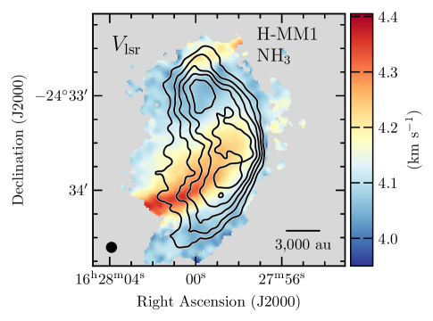
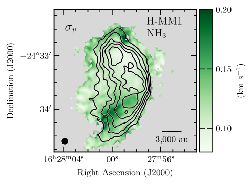
Figure 3: Centroid velocity and velocity dispersion maps derived from NH3 are shown in the left and right panels, respectively. The velocity fields show an elongated redshifted feature connecting the south-east edge and the central region of the core. The contours and the markers are as in Fig 1.

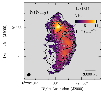
Figure 4: NH3 column density map. The central part of the map (where H2 peaks) shows a nearly constant NH3 column density, while the peak is located in the northern part of the core. The contours and the markers as in Fig 1.

3.2 Radial Velocity and Velocity Dispersion

The velocity centroids (Fig. 3-left) range from $\approx$4.0 $\rm km\,s^{-1}$ to $\approx$4.4 $\rm km\,s^{-1}$ across the core. Prominent in this distribution is a narrow feature at velocities $>$4.3 $\rm km\,s^{-1}$ that seems to connect the South-East end and the center of the core. The velocity dispersion (Fig. 3-right) is small across the map. The narrowest line, $\approx$0.09 $\rm km\,s^{-1}$, is found in the northern part of the core, whereas the largest values, $>$0.15 $\rm km\,s^{-1}$, lie in the southeast, in the region of the highest $V_{\rm LSR}$ values. The locations of large $\sigma_{\rm v}$ form a narrow strip, but the orientation of this strip deviates from that of the red-shifted $V_{\rm LSR}$ feature.

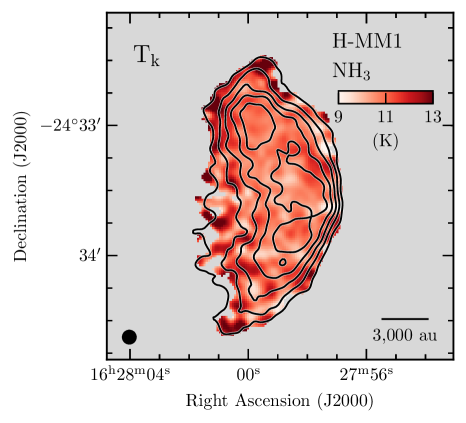
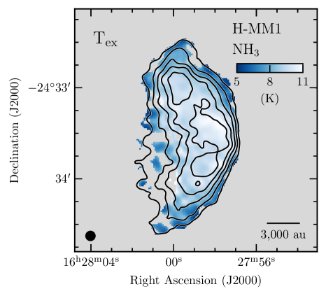
Figure 5: Kinetic and excitation temperature maps for H-MM1 are shown in the left and right panels, respectively. The contours and the markers are as in Fig 1. These maps only include pixels where the uncertainty is smaller than 1 K.

3.3 Kinetic Temperature and Excitation Temperature

The $T_{\rm k}$ distribution is almost flat in the central region, but it shows a tendency to increase toward the core boundaries (Fig. 5). The average temperature in the core center is 11 K, and it rises to $\approx$12 K at lower $\ce{NH3}$ and $\ce{H2}$ column densities (Fig. 6). The $T_{\rm ex}$ of the $\ce{NH3}(1,1)$ line varies from $\approx$5 K at the core boundaries to $\approx$11 K in the central regions. This indicates that the line is thermalized in the densest parts of the core (see also Appendix B).

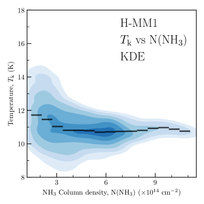
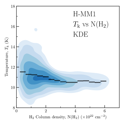
Figure 6: The Kernel Density Estimates (KDE) of the kinetic temperature as a function of NH3 and H2 column density are shown in the left and right panels, respectively. The black horizontal segments show the mean values within the column density bins. The gas temperature drops from $\approx$12 K down to $\approx 11$ K towards the highest column densities in the core.

3.4 Ammonia Abundance

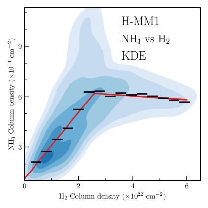
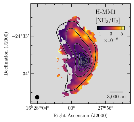
Figure 7: Depletion of NH3 in the center of H-MM1. Left: KDE comparison between NH3 and H2 column densities. This presents a positive correlation below $N(\ce{H2})<2.6\times 10^{22}$ cm^-2, whereas for higher $N(\ce{H2})$ values the NH3 column density is nearly constant or decreasing to a small degree. The black horizontal segments show the mean values within the $N(\ce{H2})$ bins. The red line shows a broken straight line fit to the data (see text). Right: Map of the fractional NH3 abundance, $X(\ce{NH3})=[\ce{NH3}]/[\ce{H2}]$, calculated as the ratio between the column densities. The NH3 abundance drops significantly in the central region, and the distribution is asymmetric so that ammonia is more abundant on the Western side of the core as compared to the Eastern side. The contours show the H2 column density starting at $1\times 10^{22}$ $\rm cm^{-2}$ and with a spacing of $1\times 10^{22}$ $\rm cm^{-2}$. The beam size and scale bar are shown as in Fig 1.

An important quantity is the molecular fractional abundance of NH3 with respect to H2, $X(\ce{NH3})=[\ce{NH3}]/[\ce{H2}]$. This quantity is key to accurately determine total H2 column densities from NH3 observations when no H2 column density map is available, while it is also important to constrain chemical models (e.g., Sipilä et al., 2019b). The $N(\ce{NH3})$ versus $N(\ce{H2})$ relation is expected to be linear where $X(\ce{NH3})$ is constant.

The comparison of all pixels with an accurate NH3 and H2 column density determinations is presented in Fig. 7-left. It shows a region with a linear rise followed by a sharp change to a nearly constant $N(\ce{NH3})$ as the $\ce{H2}$ column density increases. We have fitted a broken straight line of the form

$$N(\ce{NH3})[x]=\begin{cases}a\cdot x+b&x<x_{0}\\ c\cdot x+(a-c)\cdot x_{0}+b&x\geq x_{0}\end{cases}$$ (1)

to the data points using emcee (Foreman-Mackey et al., 2013). The results are listed in Table 1 and shown by the red curve in Fig. 7-left, while a more detailed description of the fit is given in Appendix C.

Table 1: Summary of Linear fit

Parameter	Value	Unit
$a$	$1.975_{-0.005}^{0.005}$	$\times 10^{-8}$
$b$	$1.121_{-0.008}^{0.008}$	$\times 10^{14}$ cm-2
$x_{0}$	$2.575_{-0.004}^{0.003}$	$\times 10^{22}$ cm-2
$c$	$-0.110_{-0.005}^{0.005}$	$\times 10^{-8}$

Note. — Due to the systematic calibration uncertainties of the NH3 observations, we list a 10% systematic uncertainty to $a$ and $c$ in addition to the statistical one in the text.

A different approach to estimate the molecular fractional abundance is to determine the fractional abundance at every pixel by taking the ratio of both column density estimates (see the map in Fig. 7-right). Here we see a higher $X(\ce{NH3})$ on the outskirts of the dense core, while in the central region there is a sharp fall-off in the determined fractional abundance. Both the decreasing tendency in the $N(\ce{NH3})$ versus $N(\ce{H2})$ correlation at high column densities in Fig. 7-left and the minimum in the fractional abundance seen in Fig. 7-right indicate that ammonia is strongly depleted in the center of the core.

4 Discussion

4.1 Gas Kinematics

The velocity dispersion, $\sigma_{\rm v}$, derived from NH3 observations changes only little within the core and indicates subsonic non-thermal motions. The H-MM1 core is thus a “coherent core” as termed by Barranco & Goodman (1998) and Goodman et al. (1998) (see also Pineda et al., 2010). The kinematics of H-MM1 and other coherent cores in the Ophiuchus region have been previously studied using observations with the Green Bank Telescope (GBT) by Auddy et al. (2019), Chen et al. (2019), and Choudhury et al. (2020). The thermal r.m.s. velocity of NH3 molecules at 11 K is $73\,\rm m\,s^{-1}$ in one dimension. The broadening owing to the channel width of the Hanning smoothed spectra, $130\,\rm m\,s^{-1}$, corresponds to an instrumental $\sigma$ of $52\,\rm m\,s^{-1}$ (see Appendix A of Choudhury et al. 2020). So, the median velocity dispersion, $\sigma_{\rm v}\sim 110\,\rm m\,s^{-1}$, from the present VLA observations indicates a median non-thermal dispersion of $\sigma_{\rm NT}\sim 63\,\rm m\,s^{-1}$, or a median sonic Mach number of $\sim 0.3$. This value is approximately half of that derived by Choudhury et al. (2020) for the narrow $\ce{NH3}$ line component from GBT observations with an angular resolution of $31\arcsec$.

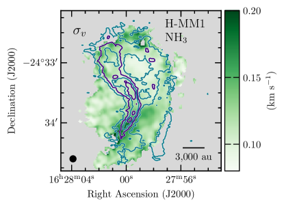
Figure 8: Velocity dispersion of $\ce{NH3}$ lines (color map) and the distribution of bright 96.7 GHz methanol emission (contours) in H-MM1. The contour levels go from 0.8 to 4.0 K $\rm km\,s^{-1}$ by steps of 0.8 K $\rm km\,s^{-1}$ and alternating between blue and purple.

The velocity dispersion attains values clearly higher than the median in a narrow region in the southeastern part of the core. This region overlaps partially with the southern “tail” of the bright $\rm CH_{3}OH$ emission mapped by Harju et al. (2020). The integrated intensity contours of four methanol lines at 96.7 GHz are overlaid onto the $\ce{NH3}$ $\sigma_{\rm v}$ map in Fig. 8. However, as can be seen in Fig. 8, methanol emission arises mostly from regions where the dispersion is close to the average. Therefore, the present data do not support the idea that efficient $\rm CH_{3}OH$ desorption is only associated with enhanced turbulence or large velocity fluctuations, lending credence to the chemical desorption scenario of methanol formation at the edge of the catastrophic CO freeze-out zone (Vasyunin et al., 2017). Perhaps it is worth to notice, though, that the most quiescent region in the northern part of the core with $\sigma_{\rm v}\sim 90\,\rm m\,s^{-1}$ (implying $\sigma_{\rm NT}<10\,\rm m\,s^{-1}$) is clearly devoid of $\rm CH_{3}OH$.

The elongated redshifted feature seen in the velocity centroid map at $V_{\rm LSR}>4.3\,\rm km\,s^{-1}$ seems to connect the compact dense core with the outer regions. This feature bears resemblance to the streamer detected using gas tracers around binary protostar Per-emb-2 (Pineda et al., 2020). We will discuss the core kinematics and the nature of this possible streamer in detail in a separate paper.

4.2 Gas Temperature

The gas temperature shows only a small drop toward the core center. The temperature 11 K in the inner parts is consistent with previous gas and dust temperature determinations using GBT and Herschel data (Harju et al., 2017; Auddy et al., 2019; Choudhury et al., 2020). The temperature profile in H-MM1 is very different from that in the well-studied prestellar core L1544, where the central temperature reaches down to $\approx 6$ K (Crapsi et al., 2007), or the starless core CB17, where the central temperature reaches down to $\approx 9.5$ K (Spear et al., 2021). The main difference is that H-MM1 is located in an environment with strong radiation field (e.g., Rawlings et al., 2013). Far-infrared radiation which penetrates the core is absorbed by dust particles, and this heating is conveyed to gas by gas-dust collisions. The density in the core, in excess of $10^{5}\,\rm cm^{-3}$, is high enough to make gas-dust thermal coupling efficient (Goldsmith, 2001; Galli et al., 2002; Ivlev et al., 2019).

4.3 Ammonia Depletion

Figure 9 shows the Kernel Density Estimates (KDE) of the fractional NH3 abundance derived. The mean fractional NH3 abundance, $[\ce{NH3}]/[\ce{H2}]_{int}$, derived as the ratio between $N(\ce{NH3})$ and $N(\ce{H2})$ is $2.7\times 10^{-8}$ (blue marker in Fig. 9), which is comparable to the values derived in other regions. However, this abundance value is higher by a factor of 3.5 compared to that derived from the single dish observations ($[\ce{NH3}]/[\ce{H2}]_{SD}=7.6\times 10^{-9}$, Harju et al. 2017), which is shown with the brown marker in Fig. 9. The fractional NH3 abundance derived from the linear fit ($[\ce{NH3}]/[\ce{H2}]_{fit}={(}1.975{\pm 0.005)}\times 10^{-8}$, $\pm$10% systematic) is shown by the red marker in Fig. 9. The fractional NH3 abundance derived for H-MM1 using the interferometric data is comparable to those derived from modelling single dish observations of L1498 and L1517 (Tafalla et al., 2004), see Table 4.3. This important difference between the interferometric and single dish results is due to the size of the depletion region, which is comparable to the single dish beam size. This highlights the crucial importance of deep spatially resolved maps of dense cores to study the depletion regions.

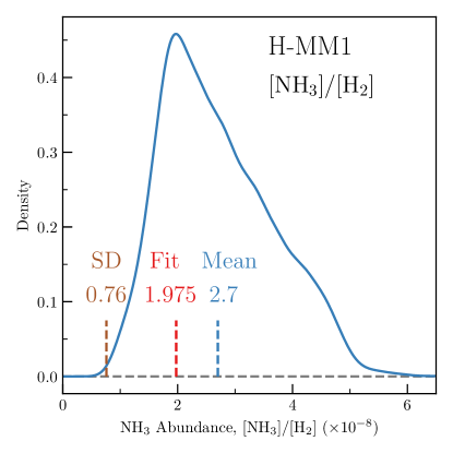
Figure 9: Probability density function estimated with KDE of the fractional NH3 abundance towards H-MM1, $[\ce{NH3}]/[\ce{H2}]$. The value estimated from single dish observations (Harju et al., 2017) is shown by the vertical brown line, $[\ce{NH3}]/[\ce{H2}]_{SD}=7.6\times 10^{-9}$. The mean value of the column density ratio is marked with a vertical blue line, $[\ce{NH3}]/[\ce{H2}]_{int}=2.7\times 10^{-8}$, and the slope of the linear fit is marked with a red line, $[\ce{NH3}]/[\ce{H2}]_{fit}={(}1.975{\pm 0.005)}\times 10^{-8}$ ($\pm$10% systematic).

The fact that $\ce{NH3}$ is depleted in the central parts of the core is evident from Fig. 7. The failure of positive correlation between $N(\ce{NH3})$ and $N(\ce{H2})$ at high column densities (Fig. 7-left), and the deficiency of ammonia in the core center (Fig. 7-right), cannot be explained by extremely high optical thicknesses. The optical thicknesses of the four satellite groups of NH3 (1,1) are clearly below 1 even toward the center of the core, implying that the drop in the derived ammonia abundance is not an artefact caused by radiative transfer effects.

According to the two-slope fit presented in Sect. 3.4, the break-point until which the fractional ammonia abundance is $1.975\times 10^{-8}$, occurs at the column density $N(\ce{H2})=2.575\times 10^{22}\,\rm cm^{-2}$. We constructed a three-dimensional model of the core by fitting a Plummer-type function to its horizontal column density profiles (cuts parallel to the right ascension axis). The inversion method is adopted from Arzoumanian et al. (2011), and it is explained in more detail in Appendix D. Using column densities derived from $8\,\rm\mu m$ absorption, the core model does not include the ambient cloud visible in the Herschel/SPIRE maps of this region. We assume that the offset, $N(\ce{NH3})\sim 10^{14}\,\rm cm^{-2}$, in the $N(\ce{NH3})$ vs. $N(\ce{H2})$ correlation shown in Fig. 7 is caused by ammonia residing in this ambient cloud. The peak density of the core model is $n(\ce{H2})=1.3\times 10^{6}\,\rm cm^{-3}$. The relationship between the densities and column densities in this model is shown in Fig. 10. In this correlation, we only include cells that have densities higher than $5\times 10^{4}\,\rm cm^{-3}$. The choice of the threshold density is based on the high excitation temperatures of the NH3 lines ($>8$ K, Fig. 5-right), which indicate that the emission is dominated by high-density gas. According to the excitation calculations presented in Shirley (2015) (their Fig. 2) for gas at $T_{\rm kin}=10$ K, the $T_{\rm ex}$ of the $\ce{NH3}(1,1)$ transition exceeds 8 K at the density $n(\ce{H2})\sim 5\times 10^{4}\,\rm cm^{-3}$. Using a lower density threshold would decrease the mean densities but leave the power law, ${\bar{n}}\propto N^{0.8}$, unchanged.

Line segments through the core having a column density around $N(\ce{H2})=2.6\times 10^{22}\,\rm cm^{-2}$ where $X(\ce{NH3})$ turns down, have an average density of $(2.1\pm 0.1)\times 10^{5}\,\rm cm^{-3}$. One can therefore assume that the depletion of $\ce{NH3}$ starts to take effect at this density, whereas at lower densities the fractional ammonia abundance is nearly constant, $2\times 10^{-8}$.

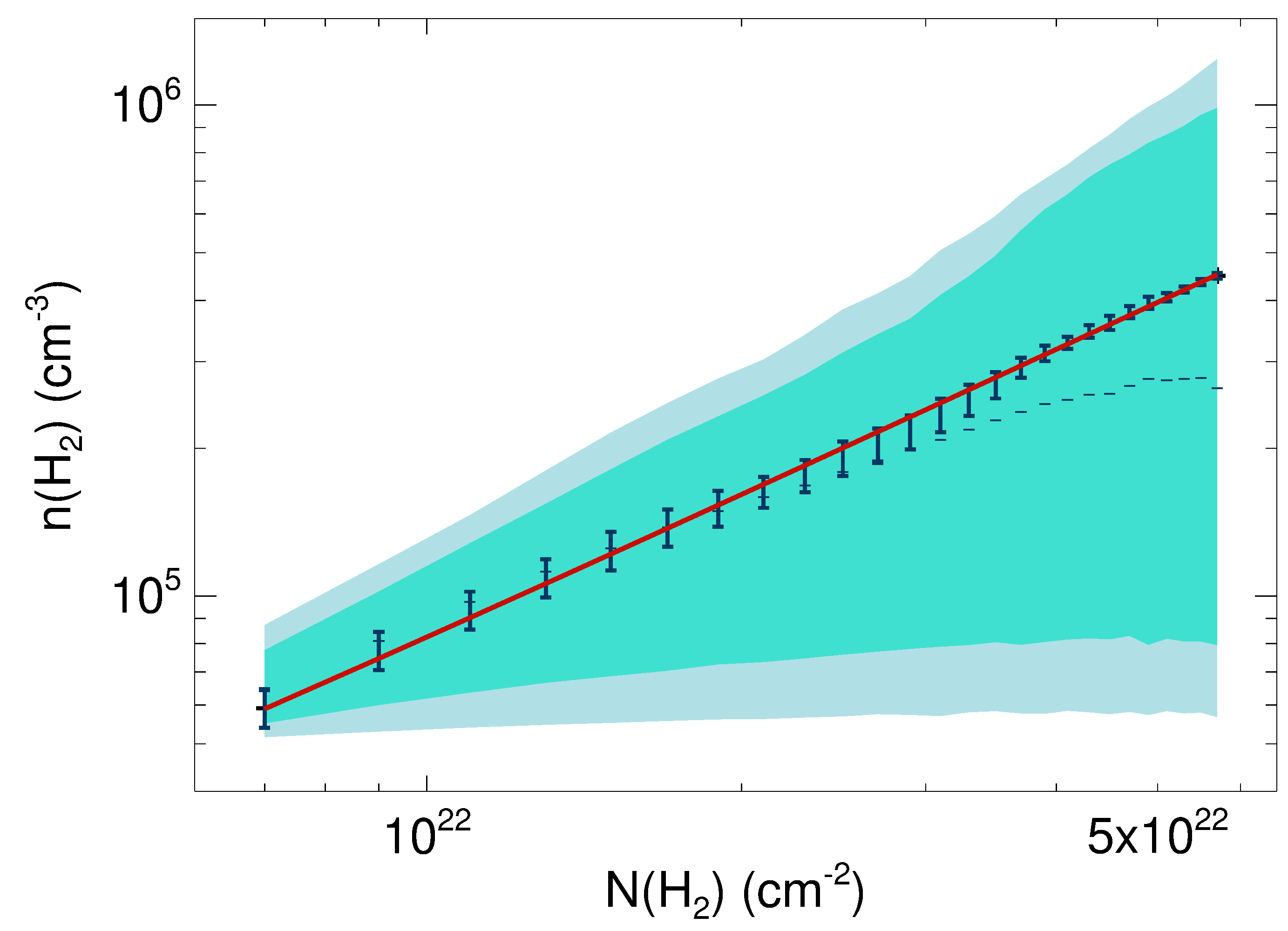
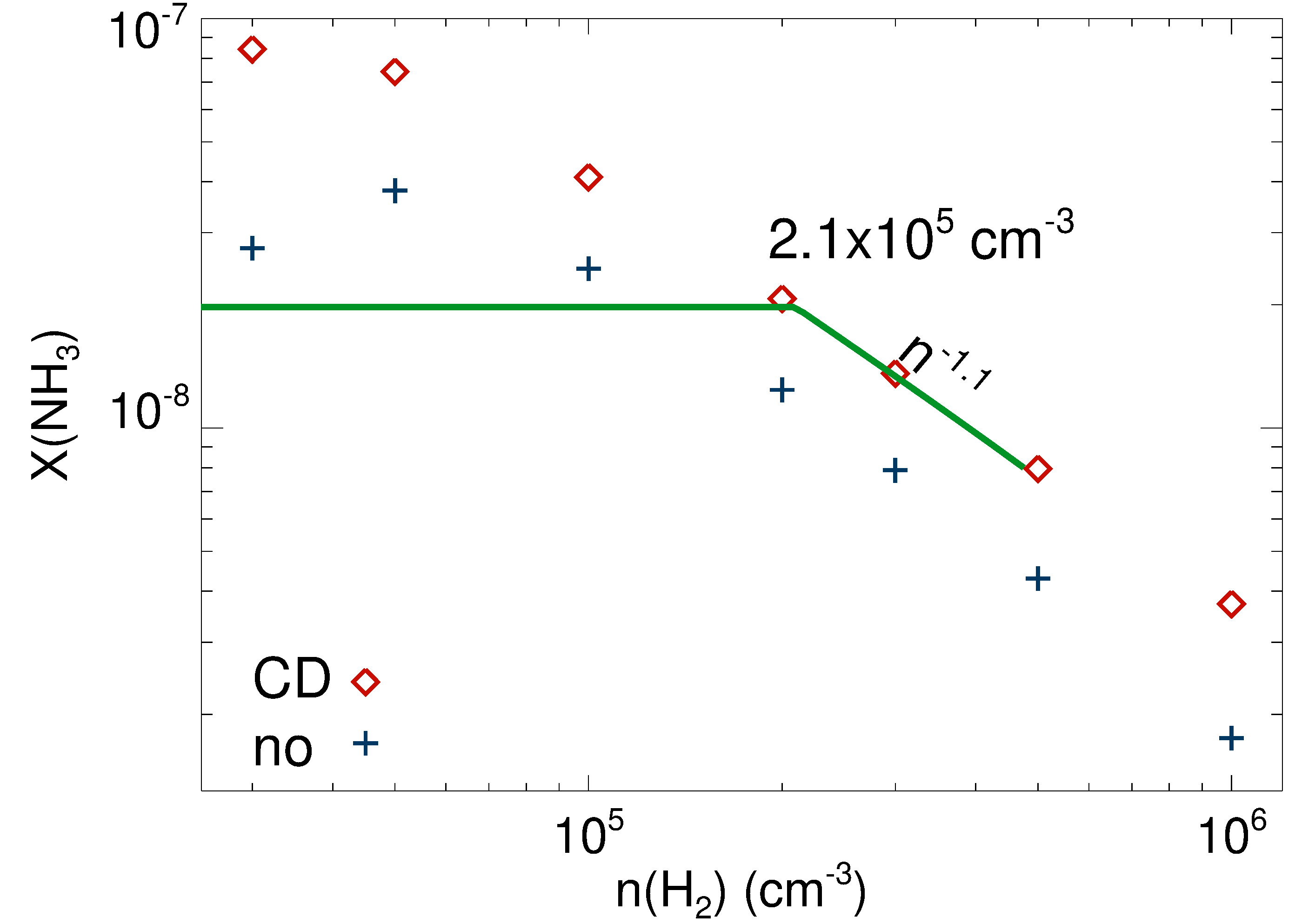
Figure 10: Left: Gas density, $n(\ce{H2})$, as a function of the $\ce{H2}$ column density in a 3-D model of the H-MM1 core (see text). The shaded regions show the densities between the 5th and 95th percentile (pale blue) and 16th and 84th percentile (turquoise) within a certain column density bin. The red line shows a linear fit to the weighted mean densities, $\bar{n}(\ce{H2})$, where each line of sight (LOS) is weighted according to standard deviation of the density ($1/\sigma_{n}^{2}$) along that LOS. The error bars correspond to the weighted sigmas of the sample densities. The median density in each $N(\ce{H2})$ bin is shown with small horizontal bars. Right: Fractional $\ce{NH3}$ abundance as a function of gas density in H-MM1. The relationship is derived by fitting a broken line to mean $\ce{NH3}$ column densities below and above the turning point $N(\ce{H2})=2.6\times 10^{22}\,\rm cm^{-2}$ (see Sect. 3.4), and using a linear fit to $\bar{n}(\ce{H2})$ vs. $N(\ce{H2})$ on the left. Also shown are predictions from our chemistry model including chemical desorption (CD, diamonds) and CD turned off (plus signs; see text).

The broken-line fit to the $N(\ce{NH3})$ vs. $N(\ce{H2})$ distribution (Sect. 3.4) and the inversion to mean densities described above, give the relationship $X(\ce{NH3})\propto n^{-1.1}$ at high densities. The dependence of the fractional $\ce{NH3}$ abundance on the density is shown in Fig. 10-right. The density threshold adopted in the conversion from column densities to average volume densities affects the break-point density in this diagram. Applying no threshold density would shift the break point to $1.0\times 10^{5}\,\rm cm^{-3}$. However, the slope of the decreasing abundance would remain the same. We note that the pivotal density as well as the fractional $\ce{NH3}$ abundance at low densities are likely to depend on the temperature, the external radiation field, and the chemical age of the core, and they probably change from core to core.

Also shown in Fig. 10-right are data points from a series of one-point chemistry models at different densities with the gas and dust temperatures fixed to 11 K. The chemistry code is described in Sect. 4.5, and the simulations used to investigate the density dependence are described in Sect. 4.6.

Table 2: Summary of Reported NH3 Abundances

Source	Method	[NH3/H2 ]	Ref.
H-MM1	Int. Col.Rat.	$2.7\times 10^{-8}$	This work
H-MM1	Int. Linear Fit	$(1.975\pm 0.005)\times 10^{-8}$	This work
H-MM1	SD Col.Rat.	$(0.76\pm 0.02)\times 10^{-8}$	1
L1498	SD Mod.	$3.4\times 10^{-8}$	2
L1517B	SD Mod.	$2.8\times 10^{-8}$	2
L1688	SD Col.Rat.	(0.3–3)$\times 10^{-8}$	3
L1544	Int. Mod.	(0.3–0.8)$\times 10^{-8}$	4

References. — (1) Harju et al. (2017), (2) Tafalla et al. (2004), (3) Friesen et al. (2017), (4) Crapsi et al. (2007).

Note. — SD = Single Dish data used; Int. = Interferometric data used.; Col.Rat. = Column Density Ratio used to determine fractional abundance; Mod. = fractional abundance constrained via radiative transfer modelling.

4.4 Chemistry of ammonia

The formation of ammonia in the interstellar gas is recapitulated in, for example, Roueff et al. (2015) and Sipilä et al. (2015). Once the NH+ ion is available, a sequence of reactions with H2 lead quickly to the ammonium ion, NH4+, which is the principal precursor of NH3. Electron recombination of NH4+ and smaller cations give the nitrogen hydrides NH, NH2 and NH3. Ammonia is expected to be the most abundant of these in dense cores. The pivotal ion, NH+, is formed by the charge transfer reaction NH + H+ -¿ NH+ + H or by the reaction N+ + ortho-H2 -¿ NH+ + H. In dark cloud conditions, the N+ ion forms by the dissociative charge transfer reaction N2 + He+ -¿ N+ + N + He (Hily-Blant et al., 2010, 2020).

In the gas, nitrogen hydrides are constantly converted to cations through charge or proton exchange reactions, and returned to neutral species in recombination reactions with electrons. The dominant ions reacting with ammonia are H+ and H3+ with approximately equal destruction rates, and the ionic species formed in these reactions, NH3+ and NH4+, are quickly returned to ammonia; NH3+ reacts with H2 to form NH4+, which gives mainly NH3 in recombination with electrons (see Fig. 2 in Sipilä et al. 2015).

Neutral nitrogen hydrides, as well as nitrogen atoms and molecular nitrogen, are also likely to be adsorbed onto dust grains, and this should eventually diminish the abundances of ammonia and related species, unless they are returned into the gas to the same degree. The accreted N atoms, and the NH and NH2 radicals, are efficiently hydrogenated to NH3, and most nitrogen in interstellar ices is probably bound to ammonia. As a consequence, ammonia is much more abundant in the icy mantles of dust grains than in the gas phase, and the ice mantles constitute the biggest ammonia reservoir in dense molecular clouds. In quiescent, shielded regions, the most important mechanisms releasing part of this ammonia probably are the cosmic-ray-induced desorption (e.g., Leger et al., 1985) and reactive desorption (e.g., Garrod et al., 2006). At very high densities, where the accretion timescale is short, the gas-phase abundance of ammonia probably depends on the balance between accretion and desorption.

4.5 Chemical Modeling

To aid the interpretation of the present observational results which indicate strong depletion of ammonia, we simulated the chemistry of NH3 in H-MM1 using our rate-equation gas-grain astrochemical model (e.g., Sipilä et al., 2015, 2019a). In brief, the model solves a set of rate equations connecting chemical reactions in the gas phase and on grain surfaces. Several desorption mechanisms are considered: thermal desorption, cosmic-ray induced desorption, photodesorption, and chemical desorption. We employ a one-dimensional physical model that was constructed by extracting density and dust temperature cuts through the density peak of the three-dimensional model described in Sect. 4.3 and making these cuts symmetric with respect to the density peak by averaging. The dust temperature distribution of the three-dimensional model was calculated by exposing the density model to an external radiation field composed of a) diffuse isotropic interstellar radiation, and b) radiation from B-type stars located $\sim$1 pc west of the core. The intensities of these components were adjusted until the 850 $\rm\mu m$ surface brightness map from the model agreed with the SCUBA-2 map and the average dust temperature map agreed with the color temperature $T_{\rm C}$ map derived from Herschel. We discretized the physical model into a series of points, and ran the chemical simulations separately in each point to obtain time- and radially-dependent NH3 abundance profiles. We employ here the same initial chemical abundances and other chemical model parameters as in Harju et al. (2017). The physical model is shown in Fig. 11, and the initial abundances are listed in Table 3.

Table 3: Initial chemical abundances (with respect to $n_{\rm H}$).

Species	Abundance
$\rm H_{2}$	$5.00\times 10^{-1}\,{}^{(a)}$
$\rm He$	$9.00\times 10^{-2}$
$\rm C^{+}$	$7.30\times 10^{-5}$
$\rm N$	$5.30\times 10^{-5}$
$\rm O$	$1.76\times 10^{-4}$
$\rm S^{+}$	$8.00\times 10^{-8}$
$\rm Si^{+}$	$8.00\times 10^{-9}$
$\rm Na^{+}$	$2.00\times 10^{-9}$
$\rm Mg^{+}$	$7.00\times 10^{-9}$
$\rm Fe^{+}$	$3.00\times 10^{-9}$
$\rm P^{+}$	$2.00\times 10^{-10}$
$\rm Cl^{+}$	$1.00\times 10^{-9}$

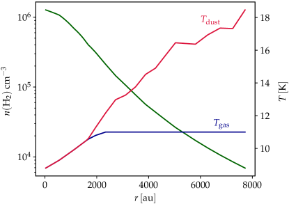
Figure 11: Physical model of H-MM1 adopted in chemical simulation: H2 number density (green) as well as the gas (blue) and dust (red) temperatures as functions of the radial distance from the center.

Based on the derived abundance profiles, we then simulated the NH3 (1,1) and (2,2) lines using the radiative transfer code LOC (Juvela, 2020). The line profiles and the column density were convolved to the angular resolution of the observations (6$\arcsec$). In Harju et al. (2017), we derived a best-fit simulation time of $3\times 10^{5}\,\rm yr$ based on fitting multiple deuterated ammonia lines. For consistency we adopt the same time here.

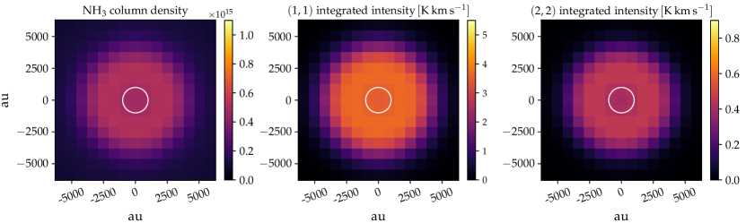
Figure 12: Simulated pNH3 column density (left), and integrated intensity ((1,1) and (2,2); middle and right panels, respectively) maps. The white circle in each panel indicates a region of 2000 au diameter.

Figure 12 shows the total NH3 column density (summed over ortho and para NH3) and integrated intensity maps obtained at this time step. The plots are displayed using the same scaling for the color bar as in Figs. 1 and 4, and we have added $10^{14}\,\rm cm^{-2}$ to the simulated column density to account for the ammonia in the outer cloud that is not included in the core model (see Sect. 4.3). The match between the model and the observations is quite good in the innermost region of the maps, which represents the volume immediately surrounding the H2 column density peak in H-MM1, even if the model somewhat under-produces the emission in both the (1,1) and the (2,2). Although not very clearly visible in the plot, both the column density and the integrated intensity maps present a dip toward the center of the core. Naturally, the model does not recover the morphology of the observed column density or integrated intensity maps outside the central region as we are using a spherically symmetric 1D model. The strength of the line emission is sensitive to uncertainties in the gas temperature in the outer core where the lines are produced.

The fractional NH3 abundance is higher near the western edge of the core than at the eastern edge (Fig. 7-right). This asymmetry can probably be attributed to the fact that the temperature gradient is steeper on the western side owing to intense radiation from that direction. We examined this hypothesis by using two one-dimensional models, which we call “east” and “west”, with the density and temperature profiles corresponding to the eastern and western sides of the core (instead of a symmetrized profile used above). The steeper rise of the temperature as a function of the distance from the core center in the “west” model was also accompanied with a steeper increase of the NH3 abundance as compared to the “east” model.

4.6 Density dependence of the ammonia abundance

As discussed in Section 4.4, the dominant gas-phase reactions involving ammonia produce closely related molecular ions that are quickly returned back to NH3. Therefore, the diminishing ammonia abundance at high densities must ultimately be caused by adsorption of NH3 and related species, mainly NH, N, and N2, onto grains. The rate at which an atom or molecule accretes onto grains is proportional to its average thermal speed and the total surface area of dust grains. The latter can be expressed as the product of the grain surface area per H atom, $\sigma_{\rm H}$ , and the total hydrogen density, $n_{\rm H}$ ($\sim 2\times n(\ce{H2})$). In other words, the accretion rate is proportional to the density.

We examined the dependence of $X(\ce{NH3})$ and related species on $n(\ce{H2})$ by employing our full chemical network. This was done by running a series of one-point models at different densities with the gas and dust temperatures fixed to 11 K. Ammonia abundances were extracted at the simulation time $3\times 10^{5}$ yr. Two different set-ups were used: one with chemical desorption (CD) and another with CD turned off. The results are shown in Fig. 13. One can see that at densities above $\sim 10^{5}\,\rm cm^{-3}$, $X(\ce{NH3})$ follows the decreasing abundances of N and N2. The slope of the $\log X(\ce{NH3})$ vs. $\log n(\ce{H2})$ curve is $-1.04\pm 0.01$ in the model with CD, and a little steeper, $\sim-1.15\pm 0.04$, when CD is turned off. The dominance of accretion leads to a density dependence close to $n^{-1}$ for neutral species, whereas electrons and light ions (H+ and H3+) show a shallower power law, $\sim n^{-0.44}$ in our models. The latter is determined by the competition between the cosmic ray ionization and neutralization in recombination reactions.

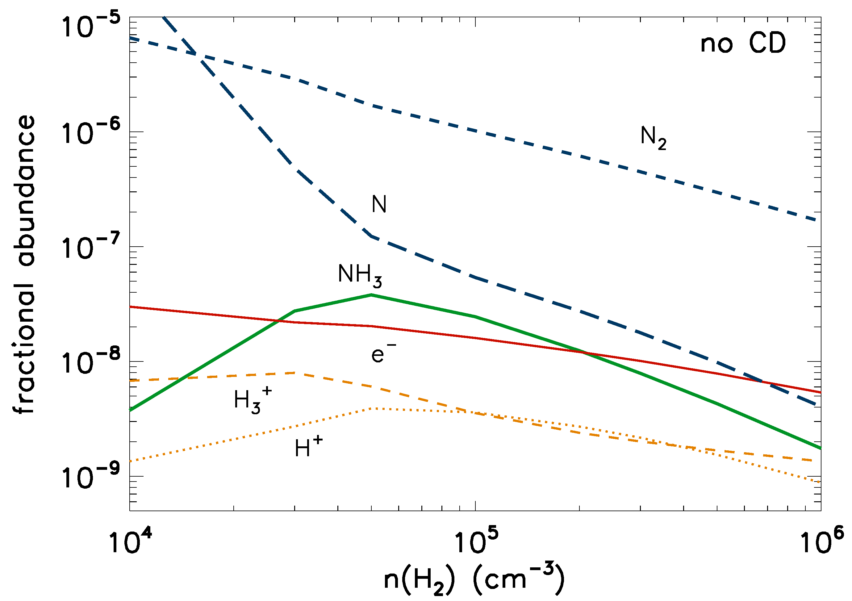
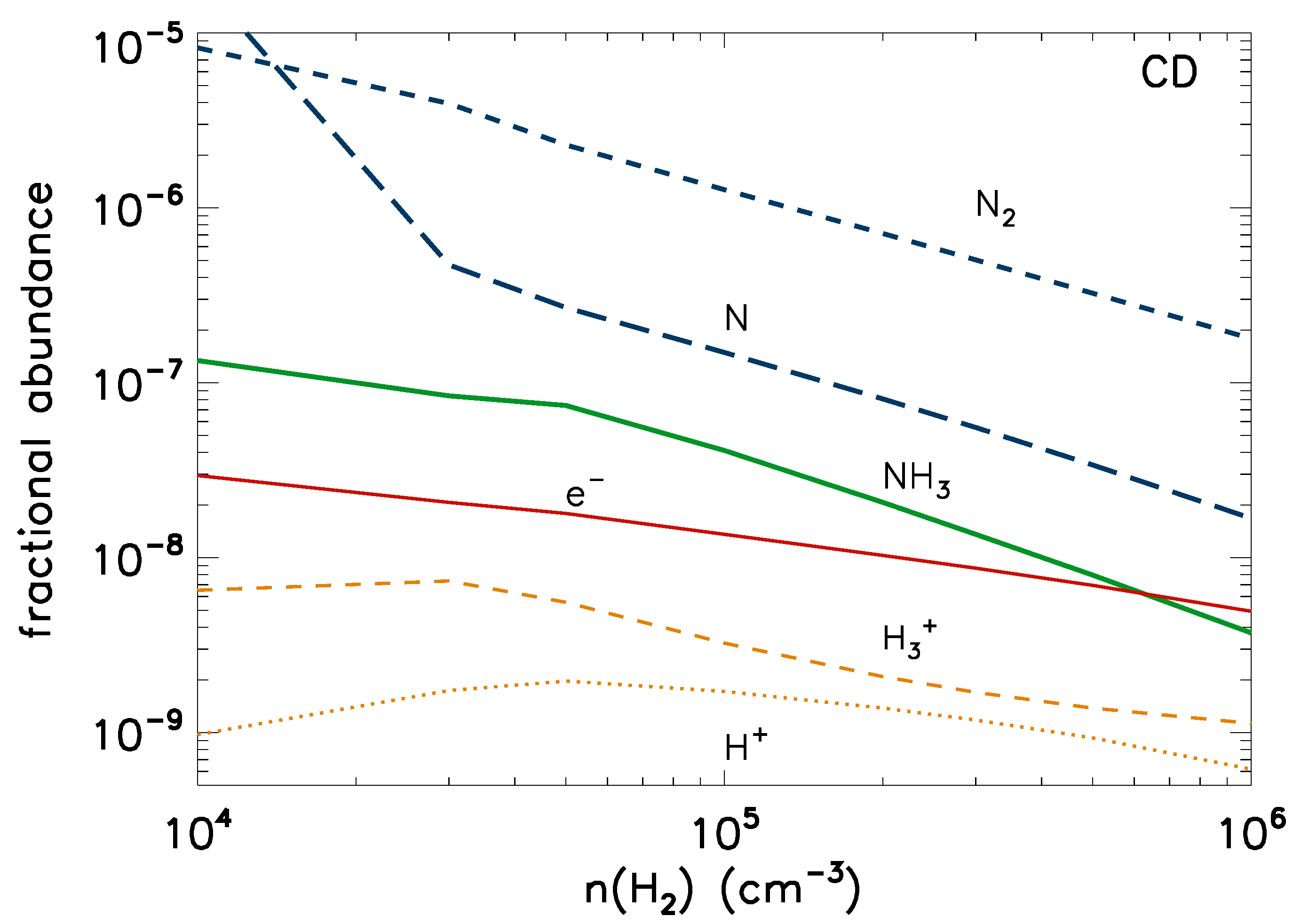
Figure 13: Modeled fractional abundances of selected species as functions of the volume density at the time $3\times 10^{5}$ yr after the beginning of the simulation. Left: A model without chemical desorption (CD). Right: A model with CD turned on, assuming that 1% of exothermic surface reactions will lead to the evaporation of the product.

According to our model, most of ammonia is to be found on dust grains, where it reaches a fractional abundance of $\sim 10^{-4}$ relative to $\ce{H2}$, and stays almost constant to the end of the simulation. Replenishment of the gas with ammonia from grains is significant when CD is effective. Consequently, $X(\ce{NH3})$ decreases more slowly and at higher densities in the model with CD than in that without CD.

Inspection of reaction rates during our chemical simulation shows that the density $5\times 10^{4}\,\rm cm^{-3}$, where the NH3 abundance turns down, is where the adsorption rate of ammonia exceeds the production of NH+ ions in the gas. In the model with CD, desorption from grains always gives more ammonia than ion-molecule reactions, but the adsorption rate surpasses the desorption rate at a density of $\sim 1\times 10^{5}\,\rm cm^{-3}$. At still higher densities, above $n(\ce{H2})=2\times 10^{5}\,\rm cm^{-3}$, a balance between the primary production of gaseous ammonia and its adsorption is established: the adsorption rate is equal to the combined rates of desorption and NH+ production up to the highest density modeled, $10^{6}\,\rm cm^{-3}$. In our CD model, desorption accounts for $\sim 80\%$ of ammonia production in this density range.

The dominant surface reaction releasing ammonia into the gas in this model is NH2^* + H^* -¿ NH3. Here we have indicated species residing on the surface with asterisks. The mentioned reaction is the end point of hydrogenation of N atoms trapped on grains. On the other hand, a majority of NH2^* molecules on the surface is formed by dissociation of $\ce{NH3^{*}}$, either by cosmic rays or by secondary photons induced by these. We can therefore present a simplified picture, where desorption is proportional to the density of ammonia residing on grains and a desorption coefficient. This picture is also valid for direct ammonia desorption caused by external agents, such as grain heating through cosmic-ray hits.

The equilibrium condition between adsorption and desorption can be written as $k_{\rm ads}\,n(\ce{NH3})=k_{\rm des}\,n(\ce{NH3^{*}})$, where $k_{\rm ads}=n_{\rm H}\sigma_{\rm H}{\bar{v}}_{\ce{NH3}}$ is the adsorption rate per molecule ($\rm s^{-1}$), ${\bar{v}}_{\ce{NH3}}$ is the mean thermal speed of ammonia molecules, and $k_{\rm des}$ is the desorption rate per molecule ($\rm s^{-1}$). The ammonia densities in the gas and on grains (per cubic centimeter) have been denoted by $n(\ce{NH3})$ and $n(\ce{NH3^{*}})$. Dividing the equilibrium equation by $n(\ce{H2})$ and re-arranging the terms one gets for the fractional ammonia abundance $X(\ce{NH3})=k_{\textrm{des}}\,X(\ce{NH3^{*}})/(\sigma_{\rm H}\,{\bar{v}}_{\ce{NH3}}\,n_{\rm H})$. According to our chemistry model, the ammonia abundance in ice exceeds the gas-phase abundance by several orders of magnitude in starless dense cores, and accretion of ammonia from the gas does not change $X(\ce{NH3^{*}})$ significantly at this stage. Assuming that also the desorption rate is approximately constant, balance between adsorption and desorption leads to an $n^{-1}$ dependence of $X(\ce{NH3})$ in the gas.

As can be seen from Fig. 10-right, both model set-ups, with or without CD, fail to reproduce the observed abundances at low densities. This probably depends on the fact that the simulation starts from atomic gas composition in physical conditions appropriate for a dense core. In reality, the dense core material has already been processed in ambient molecular cloud conditions with $n(\ce{H2})\sim 10^{3}-10^{4}\,\rm cm^{-3}$, where ammonia production on grains and in the gas has already started, and a substantial fraction of nitrogen is already incorporated in ammonia ice.

5 Conclusions

We present high spatial resolution ammonia observations with the Very Large Array and Green Bank Telescope toward the starless core H-MM1 in Ophiuchus. They indicate that ammonia has a constant fractional abundance, $X(\ce{NH3})={(}1.975{\pm 0.005)}\times 10^{-8}$ ($\pm$10% systematic), up to a column density of $N(\ce{H2})=2.575\times 10^{22}\,\rm cm^{-2}$, beyond which the abundance starts to decrease. This is direct evidence of the NH3 depletion from the gas phase, in a region of size comparable to the single dish beam size, which explains why the depletion region is only detected in deep high-angular resolution observations. By deriving a volume density model of the core we established that the critical density where NH3 starts to disappear from the gas is approximately $2\times 10^{5}\,\rm cm^{-3}$ in this core, and at higher densities $X(\ce{NH3})$ follows the power-law $X(\ce{NH3})\propto n^{-1.1}$. This tendency at high densities is reproduced by chemical simulations, and is consistent with the idea that adsorption onto grains is the main mechanism reducing the gas-phase abundances of neutral molecules in the core center. Our chemistry simulations suggest that the break-point in $X(\ce{NH3})$ versus $n(\ce{H2})$ relationship marks the density where the adsorption rate surpasses the production rate of gaseous ammonia through ion-molecule reactions and desorption. The density threshold for depletion is likely to vary from core to core because it depends on the temperature and the total grain surface area per hydrogen atom.

Appendix A Possible effects of scattering and emission at $8\,\rm\mu m$ on the $N(\ce{H2})$ map

Lefèvre et al. (2016) discussed the possible effect of dust scattering for the 8 $\mu$m absorption. With models of the cloud LDN 183, they concluded that scattering could correspond to several times $0.1\,\rm MJy\,sr^{-1}$, helping to conciliate column density estimates from mid-infrared (MIR) absorption and molecular line emission. Scattering at this level required aggregate grains with sizes much larger than in the general interstellar medium.

We examined H-MM1 similarly with 3D radiative transfer models. The models were optimised to reproduce the Herschel 250–500 $\mu$m observations under the assumption that the line-of-sight density profile is similar to that derived from the surface brightness, along a constant-declination cross section through the core centre. The external radiation field was set according to the Mathis et al. (1983) model, adopting the angular distribution on the sky from COBE/DIRBE observations (Hauser et al., 1998). We further added an energetically equal component for radiation from the equatorial west, to qualitatively account for the effect of the nearby B-type star. The optimisation of the model resulted in a scaling of the radiation field and the column-density for each map pixel. The models reproduce the Herschel surface brightness observations within 1 % at 350 $\mu$m and within $\sim 10$ % at 250 $\mu$m and 500 $\mu$m. The model optimisation was repeated for several dust models, including the Compiègne et al. (2011) dust model, the DustEM core-mantle-mantle (CMM) and ice coated aggregates (AMMI) grains (Ysard et al., 2016), and the Weingartner & Draine (2001) $R_{\rm V}=5.5$ “B” model. The estimated radiation fields were consistently slightly more than ten times the Mathis et al. (1983) values but, because of different far-infrared emissivities, the column densities varied by a factor of $\sim$3 between the dust models. In each case, we also computed 8 $\mu$m maps for the scattered light and for the emission due to stochastically heated grains. All calculations were performed with the radiative transfer program SOC (Juvela, 2019).

For all of the tested dust models, the 8 $\mu$m scattered light remained below $0.1\,\rm MJy\,sr^{-1}$. The largest value was obtained for the Weingartner & Draine (2001) grains, some $0.055\,\rm MJy\,sr^{-1}$, the AMMI grains produced less than half of this value. The CMM and AMMI models do not contain small grains and therefore result in no significant MIR emission. The level of scattered light depends not only on the scattering properties of the grains but equally on their far-infrared emissivity that, via the fits to Herschel data, determines the model column densities. The results suggest that (in the absence of very large aggregates) the scattering is not a significant factor. The 8 $\mu$m extended sky brightness in H-MM1 is of the order of $10\,\rm MJy\,sr^{-1}$, much higher than for LDN 183. Therefore, more than to the scattered light, the analysis of MIR extinction is sensitive to the assumed fraction of the extended sky brightness that originates behind the core.

For the Compiègne et al. (2011) and Weingartner & Draine (2001) dust models, the emission from stochastically heated grains at 8 $\mu$m reaches a level of a few $\rm MJy\,sr^{-1}$. However, the surface-brightness difference between the inner core and its surroundings was observed to be either positive or negative, depending on how the line-of-sight extent of the cloud was assumed to be correlated with the column density. If the abundance of small grains decreases towards the core centre, their emission is more likely to bias the MIR extinction estimates upwards than downwards.

Appendix B Comparison of NH3 excitation and kinetic temperatures

In the case of LTE, the excitation temperature and gas temperature are the same. Our determination of both these quantities allow us to directly assess how close to LTE the NH3 emission is. The comparison of the excitation to kinetic temperature ratio as a function of H2 column density is shown in Fig. 14. It shows that below $2\times 10^{22}$ $\rm cm^{-2}$ the ratio increases with column density, and at higher column densities the excitation temperature is $\approx$90% of the kinetic temperature value and close to LTE.

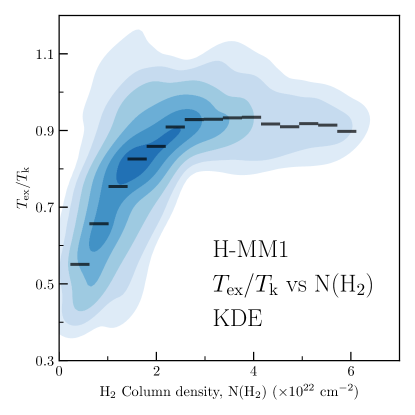
Figure 14: NH3 emission in LTE in the center of H-MM1. KDE comparison between the ratio of the excitation and kinetic temperature derived from NH3 and H2 column densities. In the case of perfect LTE the temperature ratio is 1. The data, whereas for higher $N(\ce{H2})$ values the temperature ratio is nearly constant $\approx$0.9, displays a behaviour very close to LTE. The black horizontal segments show the mean values within the $N(\ce{H2})$ bins.

Appendix C Bayesian line fit

We use emcee (Foreman-Mackey et al., 2013) to fit a broken straight line to the NH3 and H2 column densities. We use the estimated errors of $N(\ce{NH3})$ derived from the pyspeckit fit, an uninformative (uniform) prior to the variables to fit, and we run 50 chains for 15 000 steps each. The autocorrelation time is between 44 and 46 steps for the different parameters, and we use the posterior distribution after using a burn-in of 150 steps and thinning the chains by a factor of 25. The corner plot of the marginalized posterior distributions of the parameters is shown in Figure 15.

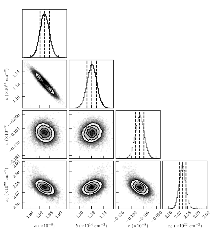
Figure 15: Corner plot of the marginalized posterior distributions for each parameter. The 16, 50, and 84 percentile of each marginalized posterior distributions are shown by the vertical dashed lines. The results are summarized in Table 1, where $a$ and $b$ are the $[\ce{NH3}]/[\ce{H2}]$ abundance (in units of $10^{-8}$) and the H2 column density offset (in units of $10^{14}\,\rm cm^{2}$) of the linear relation in the lower column density region, respectively; $x_{0}$ is the H2 column density (in units of $10^{22}\,\rm cm^{2}$) beyond which the depletion region is identified, and $c$ is the $[\ce{NH3}]/[\ce{H2}]$ abundance (in units of $10^{-8}$) in the depletion region.

Appendix D Density model of H-MM1

We estimate the density structure of the core by fitting a Plummer-type function to the cross-sectional H2 column density profiles in different positions along the north-south oriented ridge of the core. The method is adopted from Arzoumanian et al. (2011). We assume that the density distribution has circular symmetry in the plane perpendicular to the spine of the core. The latter is defined by a spline fit through local $N(\rm H_{2})$ peaks. The spline fit is shown in Figure 16a. A horizontal (constant-declination) cut through the $N(\rm H_{2})$ maximum of the core is shown in Figure 16b together with the fitted function. The function is of the form $f(\Delta y)=\frac{a}{\left[1+(\Delta y/b)^{2}\right]^{c}}$, where $\Delta y$ is the projected distance from the peak. The radial density profile, $n(r)=\frac{n_{0}}{\left[1+(r/r_{0})^{2}\right]^{\eta}}$, is obtained from this by the substitutions $\eta=c+0.5$, $r_{0}=b$, $n_{0}=a/(A_{p}r_{0})$, where $n_{0}$ is the central density and $A_{p}=\int_{-\infty}^{+\infty}{(1+u^{2})^{-\eta}}{du}$. For the cut shown in the figure, the solution is $\eta=1.6\pm 0.3$, $r_{0}=(1600\pm 300)$ au, $n_{0}=(1.30\pm 0.08)\times 10^{6}\,{\rm cm}^{-3}$. The three-dimensional density model is illustrated in Figure 16c. Here, the line of sight coincides with the negative $x$-axis, and the $y$-axis points to the equatorial west. This density model is used for the mean-density vs. column density correlation shown in Fig. 10-left.

Figure 16: a)  Spline fit through local $N(\ce{H2})$ peaks along the ridge of H-MM1. b) Horizontal cut through the $N(\ce{H2})$ maximum of the core together with a Plummer-type fit to the profile. c)  Density model of H-MM1 constructed from Plummer fits. The iso-density surfaces shown are: $n({\ce{H2}})=10^{4}\,\rm cm^{-3}$ (green), $10^{5}\,\rm cm^{-3}$ (purple), $5\times 10^{5}\,\rm cm^{-3}$ (red), and $10^{6}\,\rm cm^{-3}$ (blue). The numbers indicate angular separations in arc seconds. The distance to the object is 138.4 pc, so a separation of $100\arcsec$ corresponds to 13,840 au.

References

- Arzoumanian et al. (2011) Arzoumanian, D., André, P., Didelon, P., et al. 2011, A&A, 529, L6
- Astropy Collaboration et al. (2013) Astropy Collaboration, Robitaille, T. P., Tollerud, E. J., et al. 2013, A&A, 558, A33
- Astropy Collaboration et al. (2018) Astropy Collaboration, Price-Whelan, A. M., Sipőcz, B. M., et al. 2018, AJ, 156, 123
- Auddy et al. (2019) Auddy, S., Myers, P. C., Basu, S., et al. 2019, ApJ, 872, 207
- Barranco & Goodman (1998) Barranco, J. A., & Goodman, A. A. 1998, ApJ, 504, 207
- Bergin & Tafalla (2007) Bergin, E. A., & Tafalla, M. 2007, ARA&A, 45, 339
- Caselli et al. (1999) Caselli, P., Walmsley, C. M., Tafalla, M., Dore, L., & Myers, P. C. 1999, ApJ, 523, L165
- Caselli et al. (2022) Caselli, P., Pineda, J. E., Sipilä, O., et al. 2022, arXiv e-prints, arXiv:2202.13374
- Chen et al. (2019) Chen, H. H.-H., Pineda, J. E., Goodman, A. A., et al. 2019, ApJ, 877, 93
- Choudhury et al. (2020) Choudhury, S., Pineda, J. E., Caselli, P., et al. 2020, A&A, 640, L6
- Choudhury et al. (2021) —. 2021, A&A, 648, A114
- Compiègne et al. (2011) Compiègne, M., Verstraete, L., Jones, A., et al. 2011, A&A, 525, A103
- Crapsi et al. (2007) Crapsi, A., Caselli, P., Walmsley, M. C., & Tafalla, M. 2007, A&A, 470, 221
- di Francesco et al. (2007) di Francesco, J., Evans, N. J., I., Caselli, P., et al. 2007, in Protostars and Planets V, ed. B. Reipurth, D. Jewitt, & K. Keil, 17
- Foreman-Mackey (2016) Foreman-Mackey, D. 2016, The Journal of Open Source Software, 1, 24. https://doi.org/10.21105/joss.00024
- Foreman-Mackey et al. (2013) Foreman-Mackey, D., Hogg, D. W., Lang, D., & Goodman, J. 2013, PASP, 125, 306
- Friesen et al. (2017) Friesen, R. K., Pineda, J. E., co-PIs, et al. 2017, ApJ, 843, 63
- Galli et al. (2002) Galli, D., Walmsley, M., & Gonçalves, J. 2002, A&A, 394, 275
- Garrod et al. (2006) Garrod, R., Park, I. H., Caselli, P., & Herbst, E. 2006, FaDi, 133, 51
- Ginsburg & Mirocha (2011) Ginsburg, A., & Mirocha, J. 2011, PySpecKit: Python Spectroscopic Toolkit, , , ascl:1109.001
- Ginsburg et al. (2019) Ginsburg, A., Koch, E., Robitaille, T., et al. 2019, radio-astro-tools/spectral-cube: v0.4.4, vv0.4.4, Zenodo, doi:10.5281/zenodo.2573901
- Goldsmith (2001) Goldsmith, P. F. 2001, ApJ, 557, 736
- Goodman et al. (1998) Goodman, A. A., Barranco, J. A., Wilner, D. J., & Heyer, M. H. 1998, ApJ, 504, 223
- Harju et al. (2017) Harju, J., Daniel, F., Sipilä, O., et al. 2017, A&A, 600, A61
- Harju et al. (2020) Harju, J., Pineda, J. E., Vasyunin, A. I., et al. 2020, ApJ, 895, 101
- Hauser et al. (1998) Hauser, M. G., Arendt, R. G., Kelsall, T., et al. 1998, ApJ, 508, 25
- Hily-Blant et al. (2020) Hily-Blant, P., Pineau des Forêts, G., Faure, A., & Flower, D. R. 2020, A&A, 643, A76
- Hily-Blant et al. (2008) Hily-Blant, P., Walmsley, M., Pineau Des Forêts, G., & Flower, D. 2008, A&A, 480, L5
- Hily-Blant et al. (2010) —. 2010, A&A, 513, A41
- Hunter (2007) Hunter, J. D. 2007, Computing In Science & Engineering, 9, 90
- Ivlev et al. (2019) Ivlev, A. V., Silsbee, K., Sipilä, O., & Caselli, P. 2019, ApJ, 884, 176
- Johnstone et al. (2004) Johnstone, D., Di Francesco, J., & Kirk, H. 2004, ApJ, 611, L45
- Juvela (2019) Juvela, M. 2019, A&A, 622, A79
- Juvela (2020) —. 2020, A&A, 644, A151
- Lefèvre et al. (2016) Lefèvre, C., Pagani, L., Min, M., Poteet, C., & Whittet, D. 2016, A&A, 585, L4
- Leger et al. (1985) Leger, A., Jura, M., & Omont, A. 1985, A&A, 144, 147
- Mathis et al. (1983) Mathis, J. S., Mezger, P. G., & Panagia, N. 1983, A&A, 500, 259
- McMullin et al. (2007) McMullin, J. P., Waters, B., Schiebel, D., Young, W., & Golap, K. 2007, in Astronomical Society of the Pacific Conference Series, Vol. 376, Astronomical Data Analysis Software and Systems XVI, ed. R. A. Shaw, F. Hill, & D. J. Bell, 127
- Ortiz-León et al. (2018) Ortiz-León, G. N., Loinard, L., Dzib, S. A., et al. 2018, ApJ, 869, L33
- Ossenkopf & Henning (1994) Ossenkopf, V., & Henning, T. 1994, A&A, 291, 943
- Pagani et al. (2007) Pagani, L., Bacmann, A., Cabrit, S., & Vastel, C. 2007, A&A, 467, 179
- Pagani et al. (2005) Pagani, L., Pardo, J. R., Apponi, A. J., Bacmann, A., & Cabrit, S. 2005, A&A, 429, 181
- Parise et al. (2011) Parise, B., Belloche, A., Du, F., Güsten, R., & Menten, K. M. 2011, A&A, 526, A31
- Pattle et al. (2015) Pattle, K., Ward-Thompson, D., Kirk, J. M., et al. 2015, MNRAS, 450, 1094
- Pineda et al. (2010) Pineda, J. E., Goodman, A. A., Arce, H. G., et al. 2010, ApJ, 712, L116
- Pineda et al. (2021) Pineda, J. E., Schmiedeke, A., Caselli, P., et al. 2021, ApJ, 912, 7
- Pineda et al. (2020) Pineda, J. E., Segura-Cox, D., Caselli, P., et al. 2020, Nature Astronomy, 4, 1158
- Rawlings et al. (2013) Rawlings, M. G., Juvela, M., Lehtinen, K., Mattila, K., & Lemke, D. 2013, MNRAS, 428, 2617
- Redaelli et al. (2019) Redaelli, E., Bizzocchi, L., Caselli, P., et al. 2019, A&A, 629, A15
- Robitaille (2019) Robitaille, T. 2019, APLpy v2.0: The Astronomical Plotting Library in Python, , , doi:10.5281/zenodo.2567476. https://doi.org/10.5281/zenodo.2567476
- Robitaille & Bressert (2012) Robitaille, T., & Bressert, E. 2012, APLpy: Astronomical Plotting Library in Python, Astrophysics Source Code Library, , , ascl:1208.017
- Roueff et al. (2015) Roueff, E., Loison, J. C., & Hickson, K. M. 2015, A&A, 576, A99
- Shirley (2015) Shirley, Y. L. 2015, PASP, 127, 299
- Sipilä et al. (2019a) Sipilä, O., Caselli, P., & Harju, J. 2019a, A&A, 631, A63
- Sipilä et al. (2019b) Sipilä, O., Caselli, P., Redaelli, E., Juvela, M., & Bizzocchi, L. 2019b, MNRAS, 487, 1269
- Sipilä et al. (2015) Sipilä, O., Harju, J., Caselli, P., & Schlemmer, S. 2015, A&A, 581, A122
- Spear et al. (2021) Spear, S., Maureira, M. J., Arce, H. G., et al. 2021, ApJ, 923, 231
- Tafalla et al. (2004) Tafalla, M., Myers, P. C., Caselli, P., & Walmsley, C. M. 2004, A&A, 416, 191
- Vasyunin et al. (2017) Vasyunin, A. I., Caselli, P., Dulieu, F., & Jiménez-Serra, I. 2017, ApJ, 842, 33
- Virtanen et al. (2020) Virtanen, P., Gommers, R., Oliphant, T. E., et al. 2020, Nature Methods, 17, 261
- Walmsley et al. (2004) Walmsley, C. M., Flower, D. R., & Pineau des Forêts, G. 2004, A&A, 418, 1035
- Weingartner & Draine (2001) Weingartner, J. C., & Draine, B. T. 2001, ApJ, 548, 296
- Ysard et al. (2016) Ysard, N., Köhler, M., Jones, A., et al. 2016, A&A, 588, A44