Role of slow, out-of-equilibrium modes on the dynamic structure factor near the QCD critical point

Abstract

The role of slow out of equilibrium modes (OEM), introduced to extend the validity of hydrodynamics near the QCD critical point on the power spectrum of dynamical density fluctuations has been studied. We have used the equation of motion of slow modes for the situation when the extensive nature of thermodynamics is not altered due to the introduction of OEM. We find that the extensivity condition puts an extra constraint on the coupling of OEM with the four divergence of velocity. The dynamic structure factor ($\mathscr{S}_{nn}(\mathchoice{\mbox{\boldmath$k$}}{\mbox{\boldmath$k$}}{\mbox{\boldmath$\scriptstyle k$}}{\mbox{\boldmath$\scriptscriptstyle k$}},\omega)$) in presence of the OEM shows four Lorentzian peaks asymmetrically positioned about $\omega(\text{frequency})=0$, whereas the dynamic structure factor without the presence of any OEM shows three well-known Lorentzian peaks. The width of the peaks are reduced in presence of OEM. We find that the asymmetric peaks originate due to the coupling of the out-of-equilibrium modes with the hydrodynamic modes. It is also shown that the OEM has negligible effects on $\mathscr{S}_{nn}(\mathchoice{\mbox{\boldmath$k$}}{\mbox{\boldmath$k$}}{\mbox{\boldmath$\scriptstyle k$}}{\mbox{\boldmath$\scriptscriptstyle k$}},\omega)$ if first order hydrodynamics (relativistic Navier-Stokes) is used. The introduction of OEM reduces the width of the Rayleigh peak indicating the reduction in the decay rate of the fluctuation which leads to slowing down, a well-known characteristics of the critical end point (CEP).

I Introduction

One of the outstanding issue in Relativistic High Energy Collision Experiments (RHIC-E) is to detect the Critical End Point (CEP) located at some critical baryonic chemical potential ($\mu_{c}$) and critical temperature ($T_{c}$) in the QCD (Quantum Chromodynamics) phase diagram. The existence of the CEP in QCD was suggested in Refs. Halasz et al. (1998); Barducci et al. (1994); Barducci et al. (1990a); Berges and Rajagopal (1999); Kiriyama et al. (2000) based on the effective field theoretic models and by lattice QCD simulations  Fodor and Katz (2002, 2004). The experimental search for the CEP has been taken up through the beam energy scan (BES) program at the Relativistic Heavy Ion Collider (RHIC) Aggarwal et al. (2010). The search will continue in future experiments at the Facility for Anti-proton and Ion Research (FAIR) and Nuclotron- based Ion Collider fAcility (NICA). The exact location of the CEP is not known from the first principle because of the difficulties associated with the sign problem of the spin 1/2 Dirac particle (quark) in lattice QCD calculations Gavai (2015). Some of the QCD based effective models such as NJL and PNJL predict the location of the CEP  Masayuki and Koichi (1989); Barducci et al. (1990b); Barducci et al. (1994); Kiriyama et al. (2000) but the results are dependent on the parameters of the models. However, the prediction of the location of the CEP is not the only problem. Even if the location of the CEP is predicted accurately its experimental detection is extremely challenging because the measured quantities are obtained by integration over the space-time evolution history of the fireball produced in relativistic heavy ion collisions, that is, the experimental results are superposition of all temperatures and densities through which the system passes, not only from the single point ($\mu_{c}$, $T_{c}$) of the phase diagram. The space time evolution of the fireball are studied by solving relativistic hydrodynamic equations controlling the conservation of the density of conserved quantities. The hydrodynamic modeling has been used to study the evolution of the fireball created in relativistic nuclear collisions with the inclusion of the CEP Du et al. (2021); Bleicher and Herold (2012); Aguiar et al. (2007); Nonaka and Asakawa (2005). However, the hydrodynamics breaks down near the CEP  Stephanov and Yin (2018) due to long range correlations and enhanced fluctuations Asakawa et al. (2000); Jeon and Koch (2003); Koch (2008). The CEP causes the system to linger its relaxation to equilibrium, termed as the ‘critical slowing down’ Berdnikov and Rajagopal (2000); Stanley (1987); Ma (1976). It has been shown in Ref. Stephanov and Yin (2018) that the validity of the hydrodynamics can be extended near CEP by introducing a scalar non-hydrodynamic field.

The hydrodynamics is used to describe the slowly evolving modes of the macroscopic system while the faster non-hydrodynamic modes are set by the collision dynamics at the microscopic level. The hydrodynamics can be applied to systems in local equilibrium. The time required to achieve local equilibrium is much shorter than the time required to attain global equilibrium and this separation of time scale permits the application of hydrodynamics. At the CEP the correlation length diverges leading to the divergence of the time scale for local equilibration which leads to the break down of the hydrodynamics. In other words, if the system encounters CEP then the correlation length ($\xi$) diverges and the relaxation time which evolves as $\sim\xi^{3}$, also diverges leading to critical slowing down. Consequently, the system stay away from local thermal equilibrium and the hydrodynamics becomes inapplicable. In such situation, a new variable, $\phi$ representing non-hydrodynamic mode is included in the definition of entropy along with other hydrodynamical variables to extend the validity of the hydrodynamics in the vicinity of the CEP  Stephanov and Yin (2018). The slow out-of-equilibrium modes (OEM) are not treated separately Stephanov and Yin (2018); Rajagopal et al. (2020) as they are coupled with hydrodynamic modes. In this regards, it is very important to understand the role of $\phi$ on the critical point dynamics. In the present work the effect of $\phi$ on the spectral structure will be studied using relativistic causal dissipative hydrodynamics proposed by Israel and Stewart (IS) Israel (1976). The dispersion relations for the hydrodynamic modes are governed by the set of hydrodynamic equations. The extensivity of thermodynamics restricts the coupling of slow modes with gradients of other hydrodynamic fields.

The fluctuations in condensed matter system has been extensively studied. Specifically, the power spectrum of the correlation of density fluctuations or the spectral structure ($\mathscr{S}_{nn}(\mathchoice{\mbox{\boldmath$k$}}{\mbox{\boldmath$k$}}{\mbox{\boldmath$\scriptstyle k$}}{\mbox{\boldmath$\scriptscriptstyle k$}},\omega)$) has been studied both experimentally and theoretically and shown to be crucially dependent on transport coefficients  Stanley (1987); Ma (2018); E. Reichl . The thermally excited fluctuations are governed by the the transport coefficients of the medium according to the Onsager’s hypothesis Onsager (1931). The light and neutron scatterings experiments have been performed to investigate the properties of fluctuations experimentally in condensed matter physics. The spectrum of scattered light contains separately identifiable peaks of Lorentzian distribution, called Rayleigh (R) peak Rayleigh (1881) at angular frequency, $\omega=0$, and Brillouin (B) peaks located symmetrically in the opposite side of R-peak, experimentally detected by Fleury and Boon Fleury and Boon (1969). The R-line arises from the entropy or temperature fluctuations at constant pressure, whereas B-lines arise from the pressure fluctuations at constant entropy. The width of the R-line is connected to $\kappa/(\rho C_{P})$ Stanley (1987), where $\kappa$ is the thermal conductivity, $C_{P}$ is the isobaric specific heat of the fluid with mass density, $\rho$. Therefore, if the order of divergence for $\kappa$ is weaker than $C_{P}$, then a narrow R-line appears. Since the width represents the decay rate of the fluctuation a narrow width will indicate the slower decay of fluctuation. Two Brillouin-peaks are positioned at $\pm c_{s}k$ with respect to the frequency of the incident light, where $c_{s}$ is the speed of sound and $k$ is the wave vector. The finite width of the B-line provides information about the values of transport coefficients such as shear, and bulk viscosities. The ratio of intensities of R-line to B-line is: $I_{R}/2I_{B}=C_{P}/C_{V}-1=K_{T}/K_{S}-1$, called the Landau-Placzek ratio where $K_{T}$ and $K_{S}$ are isothermal and isothermal and adiabatic compressibilities respectively. Therefore, the study of the structure factor is very useful to understand the behaviour of the fluid near the CEP as some of the transport coefficients and response functions change drastically. Near the CEP the B-peaks tend to vanish giving rise to severe modification in $\mathscr{S}_{nn}(\mathchoice{\mbox{\boldmath$k$}}{\mbox{\boldmath$k$}}{\mbox{\boldmath$\scriptstyle k$}}{\mbox{\boldmath$\scriptscriptstyle k$}},\omega)$. In QCD no external probe exists to measure such drastic change in $\mathscr{S}_{nn}(\mathchoice{\mbox{\boldmath$k$}}{\mbox{\boldmath$k$}}{\mbox{\boldmath$\scriptstyle k$}}{\mbox{\boldmath$\scriptscriptstyle k$}},\omega)$. However, it is a well-known feature of the critical phenomena that the behaviour of a large class of systems near CEP are independent of the dynamical details. Since, the CEP in QCD belongs to same universality class, $\mathscr{O}(4)$ Halasz et al. (1998); Berges and Rajagopal (1999), as that of liquid-gas critical point, the role of such slow modes can be tested in liquid-gas system, and the knowledge can be very helpful to guide the theoretical modeling relevant to the CEP of QCD. In this context the qualitative and quantitative effects of the slow modes on various physical quantities should be studied. In the present work the effects of these modes on the spectral structure of the fluctuations near the CEP  Minami and Kunihiro (2009, 2010); Hasanujjaman et al. (2021) has been investigated. More specifically, we will study role of the slow modes on the Rayleigh and Brillouin peaks of $\mathscr{S}_{nn}(\mathchoice{\mbox{\boldmath$k$}}{\mbox{\boldmath$k$}}{\mbox{\boldmath$\scriptstyle k$}}{\mbox{\boldmath$\scriptscriptstyle k$}},\omega)$. Thermal fluctuations can cause entropy production leading to fluctuation in multiplicity. However, their ensemble average is unaffected Nagai et al. (2016). Thermal fluctuations may not affect lower flow harmonics but affect their correlation. Recently, CMS collaborations have measured higher flow harmonics which again carry a strong signature of thermal fluctuations Chatrchyan et al. (2013) and hence that of CEP.

The paper is organized as follows. In the next section the expression for $\mathscr{S}_{nn}(\mathchoice{\mbox{\boldmath$k$}}{\mbox{\boldmath$k$}}{\mbox{\boldmath$\scriptstyle k$}}{\mbox{\boldmath$\scriptscriptstyle k$}},\omega)$ will be derived by including the variable, $\phi$ representing the non-hydrodynamic mode. In Sec.III the results are presented and Sec.IV is devoted to summary and discussion.

II Hydrodynamics with out-of-equilibrium modes

The evolution of fluid near the CEP within the scope of fluid dynamics can be extended by introducing an extra slow degree of freedom representing soft mode Stephanov and Yin (2018). Here we use the IS hydrodynamical model Israel (1976) in Eckart frame Eckart (1940) to study the effects of this slow degrees of freedom. The signature metric for the Minkowski space time is taken as, $g^{\mu\nu}=(-1,\,1,\,1\,,1)$. The fluid velocity field, $u^{\mu}$ is normalized as $u^{\mu}u_{\mu}=-1$. The energy-momentum and charge conservation equations are:

$$\partial_{\mu}T^{\mu\nu}=0$$ (1)

and

$$\partial_{\mu}J^{\mu}=0.$$ (2)

where,

$$T^{\mu\nu}=\epsilon u^{\mu}u^{\nu}+(P+\Pi)\Delta^{\mu\nu}+h^{\mu}u^{\nu}+u^{\mu}h^{\nu}+\pi^{\mu\nu},$$ (3)

$$J^{\mu}=nu^{\mu}+n^{\mu}\,,$$ (4)

where $q^{\mu}=h^{\mu}-n^{\mu}(\epsilon+P)/n$ is the heat flux, $h^{\mu}$ is the vector dissipation or dissipative energy flow, $u^{\mu}$ is the flow velocity, with $u_{\mu}h^{\mu}=u_{\mu}\pi^{\mu\nu}=0$, $n$ is conserved charge number density (net baryon density for RHIC-E), $n^{\mu}$ is dissipative current density, $\epsilon$ is energy density, $P$ is the pressure, $\Pi$ is the scalar dissipation or the bulk-stress, $\pi^{\mu\nu}$ is the tensor dissipation or shear stress tensor and $\Delta^{\mu\nu}=g^{\mu\nu}+u^{\mu}u^{\nu}$ is the projection operator, such that $\Delta^{\mu\nu}u_{\nu}=0$. In Eckart frame, $n^{\mu}=0$ and $q^{\mu}=h^{\mu}$. The relaxation equation for additional scalar soft mode $\phi$ is introduced as Stephanov and Yin (2018):

$$D\phi=-F_{\phi}+A_{\phi}\theta\,,$$ (5)

where, $\theta=\partial_{\mu}u^{\mu}$ and $D=u^{\mu}\partial_{\mu}$. Forms of $F_{\phi}$ and $A_{\phi}$ can be obtained by imposing second law of thermodynamics which states:

$$\partial_{\mu}s^{\mu}\geq 0\,,$$ (6)

where, $s^{\mu}$ is the entropy four current and is defined as

$$s^{\mu}=su^{\mu}+\Delta s^{\mu}\,.$$ (7)

In hydro+ formalism, the partial equilibrium entropy gets separate contribution from the slow modes represented by, $\phi$. The change in entropy density due to the introduction the scalar field, $\phi$ is given by,

$$ds_{+}=\beta_{+}d\epsilon-\alpha_{+}dn-\pi d\phi\,,$$ (8)

where, $\pi$ is the ‘energy cost’ for addition of $\phi$ modes in the system can be called the corresponding chemical potential. Here $\alpha_{+}=\mu_{+}/T$, where, $T$ is the temperature $\mu_{+}$ is the chemical potential.

The role of non-hydrodynamic mode on the extensivity condition was ignored in earlier calculations. In the present work it is found that, this condition is important for determining the form of $A_{\phi}$. From here onward, we drop the subscript “$+$” and write the following relations in presence of $\phi$ as:

$$dP = sdT+nd\mu+\phi d\pi\,,$$ (9)

$$sT = \epsilon+P-\mu n-\pi\phi\,.$$ (10)

The equation for the soft mode is already of relaxation type in its form, therefore, the coupling of slowly evolving soft modes at first order is adequate to maintain causality. The coupling with the soft mode at first order can be achieved as follows:

$$\partial_{\mu}s^{\mu}=(F_{\phi}-b\partial_{\mu}q^{\mu})\pi-q^{\mu}\partial_{\mu}(\beta+b\pi)-\beta(\partial_{\mu}u_{\nu})\Delta T^{\mu\nu}+\partial_{\mu}(\Delta s^{\mu}+\beta q^{\mu}+b\pi q^{\mu})+S_{n}\theta\,,$$ (11)

where $b$ represents the coupling strength and

$$S_{n}=s-\beta(\epsilon+P)+\mu\beta n+\pi A_{\phi}\,.$$ (12)

In the Eckart frame the soft mode couples with the heat flux. $\partial_{\mu}s^{\mu}\geq 0$ can be satisfied, with $S_{n}=0$ and redefinition of $\pi$, $q^{\mu}$, $\Delta T^{\mu\nu}$ and $s^{\mu}$, therefore, we have

$$\Delta s^{\mu}=-\beta q^{\mu}-b\pi q^{\mu}\,,$$ (13)

and

$$q^{\mu} = -\kappa T[Du^{\mu}-\frac{1}{\beta}\Delta^{\mu\nu}\partial_{\nu}(\beta+b\pi)]\,,$$ (14)

$$F_{\phi} = \gamma\pi-b\partial_{\mu}[\kappa TDu^{\mu}-\frac{\kappa}{\beta}\Delta^{\mu\nu}\partial_{\nu}(\beta+b\pi)]\,,$$ (15)

where the proportionality constants $\kappa\geq 0$, $\gamma\geq 0$ are respectively thermal conductivity and relaxation rate of slow modes. Comparison of Eqs.(10) and (12) gives $A_{\phi}=\phi$ for $S_{n}=0$. Therefore, the modified equations for fluxes in the second order IS theory with the coupling to soft modes read as follows:

$$\Pi=-\frac{1}{3}\zeta\Big{[}\partial_{\mu}u^{\mu}+\beta_{0}D\Pi-\tilde{\alpha}_{0}\partial_{\mu}q^{\mu}\Big{]}\,,$$

$$q^{\mu}=-\kappa T\Delta^{\mu\nu}\Big{[}\beta\partial_{\nu}(T+b\pi)+Du_{\nu}+\beta_{1}Dq_{\nu}-\tilde{\alpha}_{0}\partial_{\nu}\Pi-\tilde{\alpha}_{1}\partial_{\lambda}\pi^{\lambda}_{\nu}\Big{]}\,,$$

$$\pi^{\mu\nu}=-2\eta\Big{[}\Delta^{\mu\nu\rho\lambda}\partial_{\rho}u_{\lambda}+\beta_{2}D\pi^{\mu\nu}-\tilde{\alpha}_{1}\Delta^{\mu\nu\rho\lambda}\partial_{\rho}q_{\lambda}\Big{]}\,,$$ (16)

with constants of proportionality $\eta\geq 0$, $\zeta\geq 0$ where $\eta$ and $\zeta$ are the shear and bulk viscous coefficients respectively. The quantities, $\tilde{\alpha_{0}}$ and $\tilde{\alpha_{1}}$ are coupling coefficients, $\beta_{0},\tilde{\beta_{1}},\beta_{2}$ are relaxation coefficients. The relations of $\beta_{0},\tilde{\beta_{1}}$ and $\beta_{2}$ to the relaxation time scales are given by  Muronga (2004, 2002):

$$\tau_{\Pi}=\zeta\beta_{0},\,\,\,\,\tau_{q}=\kappa T\beta_{1},\,\,\,\,\tau_{\pi}=2\eta\beta_{2}\,,$$ (17)

The coupling coefficients, which couple to heat flux, and bulk pressure $(l_{q\Pi},l_{\Pi q})$, the heat flux, and shear tensor $(l_{q\pi},l_{\pi q})$, are related to the relaxation lengths by the following relations,

$$l_{\Pi q}=\zeta\alpha_{0},\,\,\,\,l_{q\Pi}=\kappa T\alpha_{0},\,\,\,\,l_{q\pi}=\kappa T\alpha_{1},\,\,\,\,l_{\pi q}=2\eta\alpha_{1}~{}.$$ (18)

The expressions for relaxation and coupling coefficients are taken from Ref. Hasanujjaman et al. (2021).

II.1 Linearized equations and the dynamic structure factor

Next we linearize the hydrodynamic equations for small deviations from equilibrium field quantities. We assume $\mathscr{Q}=\mathscr{Q}_{0}+\mathscr{\delta Q}$, where $\mathscr{Q}$, $\mathscr{Q}_{0}$ and $\delta\mathscr{Q}$ represents hydrodynamic variables, its average value and the fluctuation respectively. $\mathscr{Q}_{0}=0$ is its average value for dissipative degrees of freedom and $u_{0}^{\mu}=(-1,\,0,\,0,\,0)$ and $\delta u^{\mu}=(0,\,\delta\mathchoice{\mbox{\boldmath$u$}}{\mbox{\boldmath$u$}}{\mbox{\boldmath$\scriptstyle u$}}{\mbox{\boldmath$\scriptscriptstyle u$}})$.

In the linearized domain the equations of motion read as:

$$0 = -\frac{\partial\delta\epsilon}{\partial t}-(\epsilon_{0}+P_{0})+\mathchoice{\mbox{\boldmath$\nabla$}}{\mbox{\boldmath$\nabla$}}{\mbox{\boldmath$\scriptstyle\nabla$}}{\mbox{\boldmath$\scriptscriptstyle\nabla$}}\cdot\delta\mathchoice{\mbox{\boldmath$u$}}{\mbox{\boldmath$u$}}{\mbox{\boldmath$\scriptstyle u$}}{\mbox{\boldmath$\scriptscriptstyle u$}}-\mathchoice{\mbox{\boldmath$\nabla$}}{\mbox{\boldmath$\nabla$}}{\mbox{\boldmath$\scriptstyle\nabla$}}{\mbox{\boldmath$\scriptscriptstyle\nabla$}}\cdot\delta\mathchoice{\mbox{\boldmath$q$}}{\mbox{\boldmath$q$}}{\mbox{\boldmath$\scriptstyle q$}}{\mbox{\boldmath$\scriptscriptstyle q$}}\,,$$ (19a)

$$0 = -(\epsilon_{0}+P_{0})\frac{\partial}{\partial t}\delta u^{i}-\partial^{i}(\delta P+\delta\Pi)+\frac{\partial}{\partial t}\delta q^{i}-\partial_{j}\Pi^{ij}\,,$$ (19b)

$$0 = -\frac{\partial}{\partial t}\delta n-n_{0}\mathchoice{\mbox{\boldmath$\nabla$}}{\mbox{\boldmath$\nabla$}}{\mbox{\boldmath$\scriptstyle\nabla$}}{\mbox{\boldmath$\scriptscriptstyle\nabla$}}\cdot\delta\mathchoice{\mbox{\boldmath$u$}}{\mbox{\boldmath$u$}}{\mbox{\boldmath$\scriptstyle u$}}{\mbox{\boldmath$\scriptscriptstyle u$}}\,,$$ (19c)

$$0 = \delta\Pi+\frac{1}{3}\zeta[\mathchoice{\mbox{\boldmath$\nabla$}}{\mbox{\boldmath$\nabla$}}{\mbox{\boldmath$\scriptstyle\nabla$}}{\mbox{\boldmath$\scriptscriptstyle\nabla$}}\cdot\delta\mathchoice{\mbox{\boldmath$u$}}{\mbox{\boldmath$u$}}{\mbox{\boldmath$\scriptstyle u$}}{\mbox{\boldmath$\scriptscriptstyle u$}}+\beta_{0}\frac{\partial}{\partial t}\delta\Pi-\tilde{\alpha_{0}}\mathchoice{\mbox{\boldmath$\nabla$}}{\mbox{\boldmath$\nabla$}}{\mbox{\boldmath$\scriptstyle\nabla$}}{\mbox{\boldmath$\scriptscriptstyle\nabla$}}\cdot\delta\mathchoice{\mbox{\boldmath$q$}}{\mbox{\boldmath$q$}}{\mbox{\boldmath$\scriptstyle q$}}{\mbox{\boldmath$\scriptscriptstyle q$}}]\,,$$ (19d)

$$0 = \delta q^{i}+\kappa T_{0}\nabla^{i}\delta T+\kappa T_{0}\frac{\partial}{\partial t}\delta u^{i}+\kappa T_{0}\beta_{1}\frac{\partial}{\partial t}\delta q^{i}-\kappa T_{0}\tilde{\alpha}_{0}\nabla^{i}\delta\Pi-\kappa T_{0}\tilde{\alpha}_{1}\nabla_{j}\pi^{ij}\,,$$ (19e)

$$0 = \delta\pi^{ij}+2\eta\delta^{ijlm}(\partial_{l}\delta u_{m}-\tilde{\alpha}_{1}\partial_{l}\delta q_{m})+2\eta\beta_{2}\frac{\partial}{\partial t}\delta\pi^{ij}\,,$$ (19f)

$$0 = -\frac{\partial}{\partial t}\delta\phi-(\gamma+T_{0}^{2}\frac{K_{q\pi}^{2}}{\kappa}\nabla^{2})C_{\phi\pi}\delta\phi-\big{[}\gamma+(T_{0}^{2}\frac{K_{q\pi}^{2}}{\kappa}-\frac{K_{q\pi}}{C_{T\pi}})\nabla^{2}\big{]}C_{T\pi}\delta T$$ (19g)

$$-(\gamma+T_{0}^{2}\frac{K_{q\pi}}{\kappa}\nabla^{2})C_{\pi n}\delta n-T_{0}K_{q\pi}\frac{\partial}{\partial t}(\nabla_{i}\delta u^{i})+\tilde{\phi}\nabla_{i}\delta u^{i},$$

where, $K_{q\pi}=b\kappa$ and

$$C_{A\pi}=\frac{\partial\pi}{\partial A},\,\,\,\,\text{with}\,\,\,A\equiv(T,n,\phi)\,.$$ (20)

By applying Fourier-Laplace transformation i.e, $\displaystyle{\lim_{x\to\infty}}\int d^{3}x\int_{0}^{\infty}\exp[{(z-\epsilon)t-i\mathchoice{\mbox{\boldmath$k$}}{\mbox{\boldmath$k$}}{\mbox{\boldmath$\scriptstyle k$}}{\mbox{\boldmath$\scriptscriptstyle k$}}\cdot\mathchoice{\mbox{\boldmath$x$}}{\mbox{\boldmath$x$}}{\mbox{\boldmath$\scriptstyle x$}}{\mbox{\boldmath$\scriptscriptstyle x$}}}]$ from the left on the above equation and performing the integration, then, replacing $z$ by $-i\omega$ we get a set of linear equations in $\omega-k$ space given in the Appendix A.

The set of equations given in Eqs. (29)-(39) can be written in matrix form as

$$\mathds{M}\delta\mathscr{Q}=\mathscr{A}\,,$$ (21)

where, $\mathds{M}$, is an $11\times 11$ matrix, arranged row wise of coefficients of $\delta n,\delta T,\delta u_{||},\delta u_{\perp},\delta\Pi,\delta q_{||}$,
$\delta q_{\perp},\delta\pi_{||\,||},\delta\pi_{||\,\perp},\delta\pi_{\perp\,\perp}$, and $\delta\phi$ respectively The set of linear equations can be solved as

$$\delta\mathscr{Q}=\mathds{M}^{-1}\mathscr{A}\,,$$ (22)

In the present work we are interested in evaluating the two point correlation of density fluctuation. The solution of the set of equations represented by Eq. (22) leads to the following expression for density fluctuation ($\delta n$),

$$\delta n(\mathchoice{\mbox{\boldmath$k$}}{\mbox{\boldmath$k$}}{\mbox{\boldmath$\scriptstyle k$}}{\mbox{\boldmath$\scriptscriptstyle k$}},\omega)=\mathds{M}^{-1}_{11}\big{[}-\big{(}\frac{\partial{\epsilon}}{\partial n}\big{)}\delta n(\mathchoice{\mbox{\boldmath$k$}}{\mbox{\boldmath$k$}}{\mbox{\boldmath$\scriptstyle k$}}{\mbox{\boldmath$\scriptscriptstyle k$}},0)-\big{(}\frac{\partial{\epsilon}}{\partial T}\big{)}\delta T(\mathchoice{\mbox{\boldmath$k$}}{\mbox{\boldmath$k$}}{\mbox{\boldmath$\scriptstyle k$}}{\mbox{\boldmath$\scriptscriptstyle k$}},0)-\big{(}\frac{\partial{\epsilon}}{\partial\phi}\big{)}\delta\phi(\mathchoice{\mbox{\boldmath$k$}}{\mbox{\boldmath$k$}}{\mbox{\boldmath$\scriptstyle k$}}{\mbox{\boldmath$\scriptscriptstyle k$}},0)\Big{]}-\mathds{M}^{-1}_{14}\big{[}-\delta n(\mathchoice{\mbox{\boldmath$k$}}{\mbox{\boldmath$k$}}{\mbox{\boldmath$\scriptstyle k$}}{\mbox{\boldmath$\scriptscriptstyle k$}},0)\Big{]}.$$ (23)

Now we define the correlation of density fluctuations, as $\mathscr{S^{\prime}}_{nn}(\mathchoice{\mbox{\boldmath$k$}}{\mbox{\boldmath$k$}}{\mbox{\boldmath$\scriptstyle k$}}{\mbox{\boldmath$\scriptscriptstyle k$}},\omega)$ by the following expression:

$$\mathscr{S^{\prime}}_{nn}(\mathchoice{\mbox{\boldmath$k$}}{\mbox{\boldmath$k$}}{\mbox{\boldmath$\scriptstyle k$}}{\mbox{\boldmath$\scriptscriptstyle k$}},\omega)=\Big{<}\delta n(\mathchoice{\mbox{\boldmath$k$}}{\mbox{\boldmath$k$}}{\mbox{\boldmath$\scriptstyle k$}}{\mbox{\boldmath$\scriptscriptstyle k$}},\omega)\delta n(\mathchoice{\mbox{\boldmath$k$}}{\mbox{\boldmath$k$}}{\mbox{\boldmath$\scriptstyle k$}}{\mbox{\boldmath$\scriptscriptstyle k$}},0)\Big{>}\,.$$ (24)

Since, the correlation between two independent thermodynamic variables, say, $\mathscr{Q}_{i}$ and $\mathscr{Q}_{j}$ vanishes i.e

$$\Big{<}\delta\mathscr{Q}_{i}(\mathchoice{\mbox{\boldmath$k$}}{\mbox{\boldmath$k$}}{\mbox{\boldmath$\scriptstyle k$}}{\mbox{\boldmath$\scriptscriptstyle k$}},\omega)\delta\mathscr{Q}_{j}(\mathchoice{\mbox{\boldmath$k$}}{\mbox{\boldmath$k$}}{\mbox{\boldmath$\scriptstyle k$}}{\mbox{\boldmath$\scriptscriptstyle k$}},0)\Big{>}=0,\,\,\,\,i\neq j\,.$$ (25)

Therefore, $\mathscr{S}^{{}^{\prime}}_{nn}$ can be written as

$$\mathscr{S}^{{}^{\prime}}_{nn}(\mathchoice{\mbox{\boldmath$k$}}{\mbox{\boldmath$k$}}{\mbox{\boldmath$\scriptstyle k$}}{\mbox{\boldmath$\scriptscriptstyle k$}},\omega)=-\Big{[}\big{(}\frac{\partial{\epsilon}}{\partial n}\big{)}\mathds{M}^{-1}_{11}-\mathds{M}^{-1}_{14}\Big{]}\Big{<}\delta n(\mathchoice{\mbox{\boldmath$k$}}{\mbox{\boldmath$k$}}{\mbox{\boldmath$\scriptstyle k$}}{\mbox{\boldmath$\scriptscriptstyle k$}},0)\delta n(\mathchoice{\mbox{\boldmath$k$}}{\mbox{\boldmath$k$}}{\mbox{\boldmath$\scriptstyle k$}}{\mbox{\boldmath$\scriptscriptstyle k$}},0)\Big{>}\,,$$ (26)

The final expression for the $\mathscr{S}_{nn}(\mathchoice{\mbox{\boldmath$k$}}{\mbox{\boldmath$k$}}{\mbox{\boldmath$\scriptstyle k$}}{\mbox{\boldmath$\scriptscriptstyle k$}},\omega)$ can be obtained as:

$$\mathscr{S}_{nn}(\mathchoice{\mbox{\boldmath$k$}}{\mbox{\boldmath$k$}}{\mbox{\boldmath$\scriptstyle k$}}{\mbox{\boldmath$\scriptscriptstyle k$}},\omega)=\frac{\mathscr{S}^{{}^{\prime}}_{nn}(\mathchoice{\mbox{\boldmath$k$}}{\mbox{\boldmath$k$}}{\mbox{\boldmath$\scriptstyle k$}}{\mbox{\boldmath$\scriptscriptstyle k$}},\omega)}{\Big{<}\delta n(\mathchoice{\mbox{\boldmath$k$}}{\mbox{\boldmath$k$}}{\mbox{\boldmath$\scriptstyle k$}}{\mbox{\boldmath$\scriptscriptstyle k$}},0)\delta n(\mathchoice{\mbox{\boldmath$k$}}{\mbox{\boldmath$k$}}{\mbox{\boldmath$\scriptstyle k$}}{\mbox{\boldmath$\scriptscriptstyle k$}},0)\Big{>}}=-\Big{[}\big{(}\frac{\partial{\epsilon}}{\partial n}\big{)}\mathds{M}^{-1}_{11}-\mathds{M}^{-1}_{14}\Big{]}\,.$$ (27)

This is the spectral correlation in density fluctuation with the inclusion of the extra degree of freedom, $\phi$.

III Results and discussion

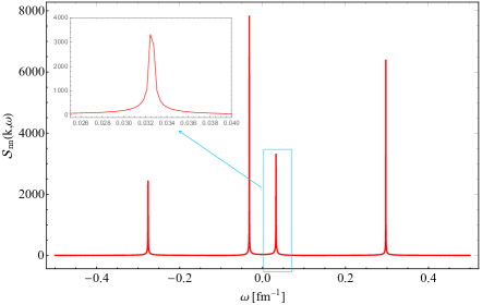
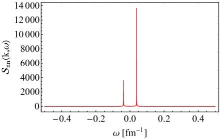
Figure 1: (Color online) (a) Variation of $\mathscr{S}_{nn}(\mathchoice{\mbox{\boldmath$k$}}{\mbox{\boldmath$k$}}{\mbox{\boldmath$\scriptstyle k$}}{\mbox{\boldmath$\scriptscriptstyle k$}},\omega)$ with $\omega$ for $k=0.1\,fm^{-1}$ and $\eta/s=\zeta/s=\kappa T/s=1/4\pi$, when the system is away from CEP ($r=0.2$). The peaks are appearing as very narrow due to the scale chosen along x-axis, change in x-axis scale makes the width visible (see the inset for the R-peak). (b) The system is close to the CEP ($r=0.01$). The results are obtained with the EoS containing the CEP and the transport coefficients, thermodynamic response function and the relaxation coefficients are estimated from the scaling behaviour.

The aim of this work is to find out the spectral structure of density fluctuation within the scope of relativistic causal hydrodynamics with its validity extended near the CEP by introducing a scalar field as discussed above. The effect of the CEP is taken into consideration through an Equation of State (EoS), containing the critical point. The EoS is constructed from the universality hypothesis which suggests that the CEP of the QCD belongs to same universality class as the 3D Ising model. We do not repeat the discussion on the construction of the EoS here but refer to the appropriate literature Parotto et al. (2020); Nonaka and Asakawa (2005); Hasanujjaman et al. (2020, 2021) for details. The behaviour of various transport coefficients and response functions play crucial roles to determine the structure factor in the presence of the CEP. The scaling behaviour of various transport coefficients and thermodynamic functions near the CEP have been taken Kapusta and Torres-Rincon (2012); Guida and Zinn-Justin (1997); Rajagopal and Wilczek (1993) into account by using the following relations:

$$\kappa_{T}=\kappa_{T}^{0}|r|^{-\gamma^{\prime}},C_{V}=C_{0}|r|^{-\alpha},C_{P}=\frac{\kappa_{0}T_{0}}{n_{0}}\Big{(}\frac{\partial P}{\partial T}\Big{)}^{2}_{n}|r|^{-\gamma^{\prime}},$$

$$c^{2}_{s}=\frac{T_{0}}{n_{0}h_{0}C_{0}}\Big{(}\frac{\partial P}{\partial T}\Big{)}^{2}_{n}|r|^{\alpha},\alpha_{p}=\kappa_{0}\Big{(}\frac{\partial P}{\partial T}\Big{)}_{n}|r|^{-\gamma^{\prime}}$$

$$\eta=\eta_{0}|r|^{1+a_{\kappa}/2-\gamma^{\prime}},\zeta=\zeta_{0}|r|^{-\alpha_{\zeta}},\kappa=\kappa_{0}|r|^{-a_{\kappa}}\,,$$ (28)

where $r=(T-T_{c})/T_{c}$ is the reduced temperature and $\alpha,\,\gamma^{\prime},\,a_{\zeta},\,a_{\kappa}$ are the critical exponents. Here $\alpha=0.11$ and $\gamma^{\prime}=1.2$. We take the values $a_{\zeta}=\nu d-\alpha=1.78$ (here, $d=3,\nu=0.63$), and $a_{\kappa}=0.63$. The partial derivative, $\left(\frac{\partial P}{\partial T}\right)_{n}$ has been evaluated by using the EoS for consistency. The critical behaviours of the second-order coupling and relaxation coefficients of the IS hydrodynamics have also been taken into account (see Hasanujjaman et al. (2021) for details).

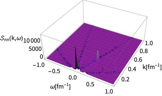
Figure 2: (Color online) Variation of $\mathscr{S}_{nn}(\mathchoice{\mbox{\boldmath$k$}}{\mbox{\boldmath$k$}}{\mbox{\boldmath$\scriptstyle k$}}{\mbox{\boldmath$\scriptscriptstyle k$}},\omega)$ with $\omega$ and $k$ for $r=0.2$, i.e when the system is away from CEP.

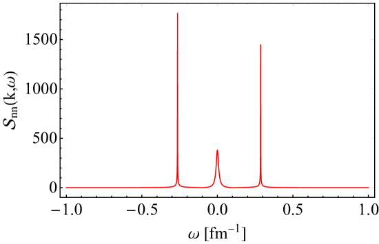
Figure 3: (Color online) Variation of $\mathscr{S}_{nn}(\mathchoice{\mbox{\boldmath$k$}}{\mbox{\boldmath$k$}}{\mbox{\boldmath$\scriptstyle k$}}{\mbox{\boldmath$\scriptscriptstyle k$}},\omega)$ with $\omega$ for $k=0.1\,fm^{-1}$ and $r=0.2$, i.e the system is away from CEP for $K_{q\pi}=0.$

In Fig.1, the variation of $\mathscr{S}_{nn}(\mathchoice{\mbox{\boldmath$k$}}{\mbox{\boldmath$k$}}{\mbox{\boldmath$\scriptstyle k$}}{\mbox{\boldmath$\scriptscriptstyle k$}},\omega)$ with $\omega$ is shown for $k=0.1$ fm^-1, when the system is away from the CEP (left panel). In absence of $\phi$, the $\mathscr{S}_{nn}(\mathchoice{\mbox{\boldmath$k$}}{\mbox{\boldmath$k$}}{\mbox{\boldmath$\scriptstyle k$}}{\mbox{\boldmath$\scriptscriptstyle k$}},\omega)$ has three peaks. These are the R-peak located at $\omega=0$ and the B-peaks located symmetrically on either sides of the R-peak. The $\mathscr{S}_{nn}(\mathchoice{\mbox{\boldmath$k$}}{\mbox{\boldmath$k$}}{\mbox{\boldmath$\scriptstyle k$}}{\mbox{\boldmath$\scriptscriptstyle k$}},\omega)$ admits four peaks in the presence of $\phi$ which is introduced to extend the validity of hydrodynamics. It is interesting to note that there is no elastic peak (R-peak) at $\omega=0$. Two away side peaks are identified as the Brillouin peaks (B-peaks). The Stokes component (left side) and the anti-Stokes component (right side) are located asymmetrically on either side of the origin with unequal magnitudes. The other peak is due to the coupling of $\phi$ with the heat flux. This profile of $\mathscr{S}_{nn}(\mathchoice{\mbox{\boldmath$k$}}{\mbox{\boldmath$k$}}{\mbox{\boldmath$\scriptstyle k$}}{\mbox{\boldmath$\scriptscriptstyle k$}},\omega)$ is different from the one evaluated earlier Hasanujjaman et al. (2021), in absence of $\phi$, where the Stokes and anti-Stokes components of equal magnitude are symmetrically located about $\omega=0$. The asymmetry in the B-peaks may arise due to the local inhomogeneity present in the system. The B-peaks arise from propagating sound modes associated with pressure fluctuations at constant entropy. In condensed matter physics, the asymmetry of the B-peaks are understood from the fact that two sound modes with different $\omega$ values, $-c_{s}k$ and $+c_{s}k$ originate from different temperature zone’s Rayleigh (1916); Zarate and Sengers (2006). The asymmetry present in Rayleigh component is exactly opposite to the Brillouin components. In the vicinity of the CEP (right panel) the $\mathscr{S}_{nn}(\mathchoice{\mbox{\boldmath$k$}}{\mbox{\boldmath$k$}}{\mbox{\boldmath$\scriptstyle k$}}{\mbox{\boldmath$\scriptscriptstyle k$}},\omega)$ shows two peaks as the B-peaks disappear due to the absorption of sound at the CEP.

In Fig. 2 the structure factor in $\omega-k$ plane has been plotted when the system is away from CEP. The structure of $\mathscr{S}_{nn}(\mathchoice{\mbox{\boldmath$k$}}{\mbox{\boldmath$k$}}{\mbox{\boldmath$\scriptstyle k$}}{\mbox{\boldmath$\scriptscriptstyle k$}},\omega)$ with non-zero $\phi$ is quite different from the case when $\phi=0$. In case of $\phi=0$ there is a $R$-peak and two $B-$ peaks at $(\omega=0)$ and $(\omega=pmc_{s}k)$ respectively with diminishing peak values as $k$ increases. However, with $\phi\neq 0$ peaks appear at non-zero $k$ values too due to the coupling of $\phi$ with other hydrodynamic fields. The symmetric structure of $\mathscr{S}_{nn}(\mathchoice{\mbox{\boldmath$k$}}{\mbox{\boldmath$k$}}{\mbox{\boldmath$\scriptstyle k$}}{\mbox{\boldmath$\scriptscriptstyle k$}},\omega)$ with R and B peaks can be reproduced when the coupling of $\pi$ (the chemical potential corresponding to the variable $\phi$) with flux $q$ is set to zero (Fig. 3).

Figure 4: (Color online) Variation of $\mathscr{S}_{nn}(\mathchoice{\mbox{\boldmath$k$}}{\mbox{\boldmath$k$}}{\mbox{\boldmath$\scriptstyle k$}}{\mbox{\boldmath$\scriptscriptstyle k$}},\omega)$ with $\omega$ for $k=0.1\,fm^{-1}$ and $r=0.2$, i.e the system is away from CEP but with higher value of $(\frac{\partial P}{\partial\phi})$. The asymmetry in the B-peaks is clearly visible.

The asymmetry in $\mathscr{S}_{nn}(\mathchoice{\mbox{\boldmath$k$}}{\mbox{\boldmath$k$}}{\mbox{\boldmath$\scriptstyle k$}}{\mbox{\boldmath$\scriptscriptstyle k$}},\omega)$ with respect to $\omega$ increases with increase in $\big{(}\partial P/\partial\phi\big{)}$. This is distinctly visible in Fig. 4 in comparison to results displayed in Fig. 1. The locations of the four peaks in $\omega$ are obtained from the dispersion relation provided in the Appendix B.

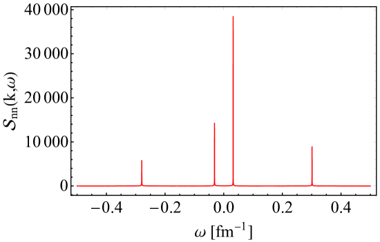
Figure 5: (Color online) Variation of $\mathscr{S}_{nn}(\mathchoice{\mbox{\boldmath$k$}}{\mbox{\boldmath$k$}}{\mbox{\boldmath$\scriptstyle k$}}{\mbox{\boldmath$\scriptscriptstyle k$}},\omega)$ with $\omega$ for $k=0.1\,fm^{-1}$ and $r=0.2$, i.e the system is away from CEP with increased $\phi$ modes in the system which increases the thermal fluctuation.

Fig. 5 displays the structure factor with increased $\phi$ mode. The height of the peaks get enhanced significantly due to the enhancement in $\phi$ value.

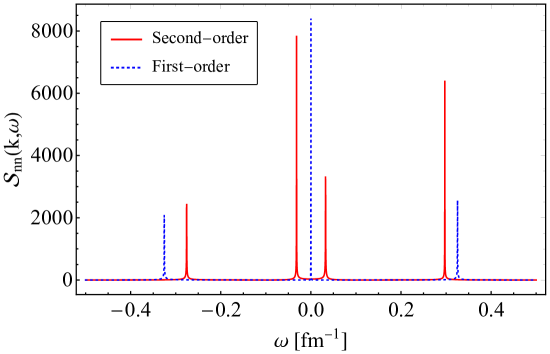
Figure 6: (Color online) Variation of $\mathscr{S}_{nn}(\mathchoice{\mbox{\boldmath$k$}}{\mbox{\boldmath$k$}}{\mbox{\boldmath$\scriptstyle k$}}{\mbox{\boldmath$\scriptscriptstyle k$}},\omega)$ with $\omega$ for $k=0.1\,fm^{-1}$ and $r=0.2$. The results for second order and first order hydrodynamics are compared here.

In Fig. 6 the structure factor for second-order hydrodynamics has been compared with first-order hydrodynamics (relativistic Navier-Stokes). Interestingly the structure factor for first-order hydrodynamics admits a R-peak at the origin and two symmetric B-peaks located on the opposite sides of the R-peak. The effects of $\phi$ seems to be inconsequential in the first-order theory because of the vanishing of various coupling and relaxation coefficients.

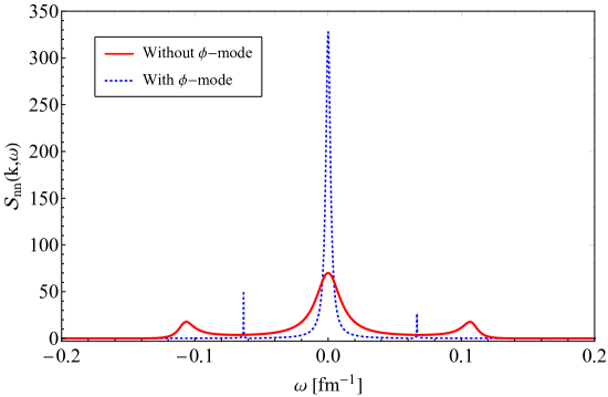
Figure 7: (Color online) Variation of $\mathscr{S}_{nn}(\mathchoice{\mbox{\boldmath$k$}}{\mbox{\boldmath$k$}}{\mbox{\boldmath$\scriptstyle k$}}{\mbox{\boldmath$\scriptscriptstyle k$}},\omega)$ with $\omega$ for $k=0.1\,fm^{-1}$ and $r=0.2$ with (dotted line) and without (solid) $\phi$ mode, when the longitudinal modes are only considered.

The $\omega$ dependence of $\mathscr{S}_{nn}(\mathchoice{\mbox{\boldmath$k$}}{\mbox{\boldmath$k$}}{\mbox{\boldmath$\scriptstyle k$}}{\mbox{\boldmath$\scriptscriptstyle k$}},\omega)$ derived from the longitudinal dispersion relation with and without $\phi$ has been depicted in Fig. 7. We find that the width of the B-peaks are small due to the introduction of the $\phi$ field (blue dashed line) and closer to the R-peak compared to the case when $\phi=0$. The rate of decay of the thermal fluctuation reflected through the width of the R-peak becomes smaller due to the introduction of the field $\phi$, that is, the decay of the fluctuation becomes slower in the presence of $\phi$. The comparison of this result with that displayed in Fig. 1 indicate that the extra peak appeared in Fig. 1 is due to the coupling of the transverse modes with $\phi$. It is interesting to note that the presence of slow modes can cause the extra peak in the dynamic structure factor in the presence of the transverse modes in the causal theory of hydrodynamics.

IV Summary and discussions

It has been shown that the validity of second-order hydrodynamics can be extended near the CEP by introducing an extra degree of freedom Stephanov and Yin (2018). Here we have derived the equation of slow modes for the situation when the extensive nature of thermodynamics is not altered due to introduction of slow modes. We find that the extensivity condition puts extra constraint on the coupling of scalar slow modes to the velocity four divergence. The role of this extra out-of-equilibrium mode on the spectral properties of dynamical density fluctuations near the QCD critical point has been investigated. The dynamical spectral structure ($\mathscr{S}_{nn}(\mathchoice{\mbox{\boldmath$k$}}{\mbox{\boldmath$k$}}{\mbox{\boldmath$\scriptstyle k$}}{\mbox{\boldmath$\scriptscriptstyle k$}},\omega)$) in presence of the out-of equilibrium modes admits four Lorentzian peaks. Whereas the dynamic structure factor without out-of-equilibrium modes admits three Lorentzians peak structure. We find that the asymmetric peaks originate due to coupling of the out-of-equilibrium modes with the hydrodynamic modes. It is also shown that the first-order hydrodynamics is unaffected by the extra variable introduced to broaden the scope of hydrodynamics. The presence of slow modes can cause the extra peak in the dynamic structure factor due to the presence of the transverse modes in the causal theory of hydrodynamics. These effects of slow modes on the dynamic structure factor may help in the experimental investigation of role of slow modes near the $\mathscr{O}(4)$ critical points other than that is expected in heavy ion collisions, such as condensed matter systems. Consequently, by virtue of universality class, the acquired knowledge on the role of slow modes from experiments on the critical point may be useful in estimating the effect of the QCD CEP through modeling the hydrodynamic evolution of system formed in heavy ion collisions near the QCD critical point. The field representing the OEM, $\phi$ plays a crucial role. It reduces the width of the distribution representing the thermal fluctuation which increases the decay time of the fluctuation.

V Acknowledgement

GS and MH acknowledge Guruprasad Kadam for fruitful discussions. GS also thanks Hiranmaya Mishra for support during part of this work. MH would also like to thank Department of Higher Education, Govt. of West Bengal, India.

Appendix A The set linear equations derived for the perturbations in $\omega-k$ space

The set of equations for the perturbations in hydrodynamic and non-hydrodynamic ($\phi$) fields in $\omega-k$ space are given in the followings. Here $\delta\epsilon(\mathchoice{\mbox{\boldmath$k$}}{\mbox{\boldmath$k$}}{\mbox{\boldmath$\scriptstyle k$}}{\mbox{\boldmath$\scriptscriptstyle k$}},\omega)$ is in the $\omega$-space and $\delta\tilde{\epsilon}(\mathchoice{\mbox{\boldmath$k$}}{\mbox{\boldmath$k$}}{\mbox{\boldmath$\scriptstyle k$}}{\mbox{\boldmath$\scriptscriptstyle k$}},t=0)$ is defined in $t$-space. Similar notation has been used for other fields.

$$i\omega\delta\epsilon(\mathchoice{\mbox{\boldmath$k$}}{\mbox{\boldmath$k$}}{\mbox{\boldmath$\scriptstyle k$}}{\mbox{\boldmath$\scriptscriptstyle k$}},\omega)+ik\delta q_{||}(\mathchoice{\mbox{\boldmath$k$}}{\mbox{\boldmath$k$}}{\mbox{\boldmath$\scriptstyle k$}}{\mbox{\boldmath$\scriptscriptstyle k$}},\omega)+ik(\epsilon_{0}+P_{0})\delta u_{||}(\mathchoice{\mbox{\boldmath$k$}}{\mbox{\boldmath$k$}}{\mbox{\boldmath$\scriptstyle k$}}{\mbox{\boldmath$\scriptscriptstyle k$}},\omega)=-\delta\tilde{\epsilon}(\mathchoice{\mbox{\boldmath$k$}}{\mbox{\boldmath$k$}}{\mbox{\boldmath$\scriptstyle k$}}{\mbox{\boldmath$\scriptscriptstyle k$}},t=0),$$ (29)

$$i\omega(\epsilon_{0}+P_{0})\delta u_{||}(\mathchoice{\mbox{\boldmath$k$}}{\mbox{\boldmath$k$}}{\mbox{\boldmath$\scriptstyle k$}}{\mbox{\boldmath$\scriptscriptstyle k$}},\omega)-ik\delta P(\mathchoice{\mbox{\boldmath$k$}}{\mbox{\boldmath$k$}}{\mbox{\boldmath$\scriptstyle k$}}{\mbox{\boldmath$\scriptscriptstyle k$}},\omega)-ik\delta\Pi(\mathchoice{\mbox{\boldmath$k$}}{\mbox{\boldmath$k$}}{\mbox{\boldmath$\scriptstyle k$}}{\mbox{\boldmath$\scriptscriptstyle k$}},\omega) + i\omega\delta q_{||}(\mathchoice{\mbox{\boldmath$k$}}{\mbox{\boldmath$k$}}{\mbox{\boldmath$\scriptstyle k$}}{\mbox{\boldmath$\scriptscriptstyle k$}},\omega)-ik\delta\pi_{||\,||}(\mathchoice{\mbox{\boldmath$k$}}{\mbox{\boldmath$k$}}{\mbox{\boldmath$\scriptstyle k$}}{\mbox{\boldmath$\scriptscriptstyle k$}},\omega)$$ (30)

$$= (\epsilon_{0}+P_{0})\tilde{\delta u}_{||}(\mathchoice{\mbox{\boldmath$k$}}{\mbox{\boldmath$k$}}{\mbox{\boldmath$\scriptstyle k$}}{\mbox{\boldmath$\scriptscriptstyle k$}},t=0)-\delta q_{||}(\mathchoice{\mbox{\boldmath$k$}}{\mbox{\boldmath$k$}}{\mbox{\boldmath$\scriptstyle k$}}{\mbox{\boldmath$\scriptscriptstyle k$}},\omega),$$

$$-i\omega(\epsilon_{0}+P_{0})\delta u_{\perp}(\mathchoice{\mbox{\boldmath$k$}}{\mbox{\boldmath$k$}}{\mbox{\boldmath$\scriptstyle k$}}{\mbox{\boldmath$\scriptscriptstyle k$}},\omega)-i\omega\delta q_{\perp}(\mathchoice{\mbox{\boldmath$k$}}{\mbox{\boldmath$k$}}{\mbox{\boldmath$\scriptstyle k$}}{\mbox{\boldmath$\scriptscriptstyle k$}},\omega)-ik\delta\pi_{\perp\,||}(\mathchoice{\mbox{\boldmath$k$}}{\mbox{\boldmath$k$}}{\mbox{\boldmath$\scriptstyle k$}}{\mbox{\boldmath$\scriptscriptstyle k$}},\omega)=(\epsilon_{0}+P_{0})\delta u_{\perp}(\mathchoice{\mbox{\boldmath$k$}}{\mbox{\boldmath$k$}}{\mbox{\boldmath$\scriptstyle k$}}{\mbox{\boldmath$\scriptscriptstyle k$}},\omega)-\tilde{\delta q}_{\perp}(\mathchoice{\mbox{\boldmath$k$}}{\mbox{\boldmath$k$}}{\mbox{\boldmath$\scriptstyle k$}}{\mbox{\boldmath$\scriptscriptstyle k$}},t=0),$$ (31)

$$i\omega\delta n(\mathchoice{\mbox{\boldmath$k$}}{\mbox{\boldmath$k$}}{\mbox{\boldmath$\scriptstyle k$}}{\mbox{\boldmath$\scriptscriptstyle k$}},\omega)+ikn_{0}\delta u_{||}(\mathchoice{\mbox{\boldmath$k$}}{\mbox{\boldmath$k$}}{\mbox{\boldmath$\scriptstyle k$}}{\mbox{\boldmath$\scriptscriptstyle k$}},\omega)=-\tilde{\delta n}(\mathchoice{\mbox{\boldmath$k$}}{\mbox{\boldmath$k$}}{\mbox{\boldmath$\scriptstyle k$}}{\mbox{\boldmath$\scriptscriptstyle k$}},t=0),$$ (32)

$$(1+i\omega\frac{1}{3}\zeta\beta_{0})\delta\Pi(\mathchoice{\mbox{\boldmath$k$}}{\mbox{\boldmath$k$}}{\mbox{\boldmath$\scriptstyle k$}}{\mbox{\boldmath$\scriptscriptstyle k$}},\omega)+ik\frac{1}{3}\zeta\delta u_{||}(\mathchoice{\mbox{\boldmath$k$}}{\mbox{\boldmath$k$}}{\mbox{\boldmath$\scriptstyle k$}}{\mbox{\boldmath$\scriptscriptstyle k$}},\omega)-ik\frac{1}{3}\zeta\tilde{\alpha}_{0}\delta q_{||}(\mathchoice{\mbox{\boldmath$k$}}{\mbox{\boldmath$k$}}{\mbox{\boldmath$\scriptstyle k$}}{\mbox{\boldmath$\scriptscriptstyle k$}},\omega)=-\frac{1}{3}\zeta\beta_{0}\tilde{\delta\Pi}(\mathchoice{\mbox{\boldmath$k$}}{\mbox{\boldmath$k$}}{\mbox{\boldmath$\scriptstyle k$}}{\mbox{\boldmath$\scriptscriptstyle k$}},t=0),$$ (33)

$$(1+i\omega\kappa T_{0}\beta_{1})\delta q_{||}(\mathchoice{\mbox{\boldmath$k$}}{\mbox{\boldmath$k$}}{\mbox{\boldmath$\scriptstyle k$}}{\mbox{\boldmath$\scriptscriptstyle k$}},\omega)+ik\kappa T_{0}\delta u_{||}(\mathchoice{\mbox{\boldmath$k$}}{\mbox{\boldmath$k$}}{\mbox{\boldmath$\scriptstyle k$}}{\mbox{\boldmath$\scriptscriptstyle k$}},\omega)+ik\big{[}\kappa-C_{T\pi}K_{q\pi}T_{0}^{2}\big{]}\delta T(\mathchoice{\mbox{\boldmath$k$}}{\mbox{\boldmath$k$}}{\mbox{\boldmath$\scriptstyle k$}}{\mbox{\boldmath$\scriptscriptstyle k$}},\omega)-ikT_{0}^{2}K_{q\pi}C_{\phi\pi}\delta\phi(\mathchoice{\mbox{\boldmath$k$}}{\mbox{\boldmath$k$}}{\mbox{\boldmath$\scriptstyle k$}}{\mbox{\boldmath$\scriptscriptstyle k$}},\omega)$$

$$-ik\kappa T_{0}\tilde{\alpha}_{0}\delta\Pi(\mathchoice{\mbox{\boldmath$k$}}{\mbox{\boldmath$k$}}{\mbox{\boldmath$\scriptstyle k$}}{\mbox{\boldmath$\scriptscriptstyle k$}},\omega)-ikT_{0}^{2}K_{q\pi}C_{n\pi}\delta n(\mathchoice{\mbox{\boldmath$k$}}{\mbox{\boldmath$k$}}{\mbox{\boldmath$\scriptstyle k$}}{\mbox{\boldmath$\scriptscriptstyle k$}},\omega)-ik\kappa T_{0}\tilde{\alpha}_{1}\delta\pi_{||\,||}(\mathchoice{\mbox{\boldmath$k$}}{\mbox{\boldmath$k$}}{\mbox{\boldmath$\scriptstyle k$}}{\mbox{\boldmath$\scriptscriptstyle k$}},\omega)$$

$$\hskip 245.71754pt=-\kappa T_{0}\tilde{\delta u}_{||}(\mathchoice{\mbox{\boldmath$k$}}{\mbox{\boldmath$k$}}{\mbox{\boldmath$\scriptstyle k$}}{\mbox{\boldmath$\scriptscriptstyle k$}},t=0)-\beta_{1}\kappa T_{0}\tilde{\delta q}_{||}(\mathchoice{\mbox{\boldmath$k$}}{\mbox{\boldmath$k$}}{\mbox{\boldmath$\scriptstyle k$}}{\mbox{\boldmath$\scriptscriptstyle k$}},t=0),$$ (34)

$$(1+i\omega\beta_{1}kT_{0})\delta q_{\perp}(\mathchoice{\mbox{\boldmath$k$}}{\mbox{\boldmath$k$}}{\mbox{\boldmath$\scriptstyle k$}}{\mbox{\boldmath$\scriptscriptstyle k$}},\omega)+i\kappa T_{0}(\omega\delta u_{\perp}(\mathchoice{\mbox{\boldmath$k$}}{\mbox{\boldmath$k$}}{\mbox{\boldmath$\scriptstyle k$}}{\mbox{\boldmath$\scriptscriptstyle k$}},\omega)-k\tilde{\alpha}_{1}\delta\pi_{\perp||}(\mathchoice{\mbox{\boldmath$k$}}{\mbox{\boldmath$k$}}{\mbox{\boldmath$\scriptstyle k$}}{\mbox{\boldmath$\scriptscriptstyle k$}},\omega)\big{)}=-\kappa T_{0}\big{[}\delta u_{\perp}(\mathchoice{\mbox{\boldmath$k$}}{\mbox{\boldmath$k$}}{\mbox{\boldmath$\scriptstyle k$}}{\mbox{\boldmath$\scriptscriptstyle k$}},0)-\beta_{1}\tilde{\delta q}_{\perp}(\mathchoice{\mbox{\boldmath$k$}}{\mbox{\boldmath$k$}}{\mbox{\boldmath$\scriptstyle k$}}{\mbox{\boldmath$\scriptscriptstyle k$}},t=0)\big{]}$$ (35)

$$(1+2i\omega\eta\beta_{2})\delta\pi_{||\,||}(\mathchoice{\mbox{\boldmath$k$}}{\mbox{\boldmath$k$}}{\mbox{\boldmath$\scriptstyle k$}}{\mbox{\boldmath$\scriptscriptstyle k$}},\omega)+ik\frac{4}{3}\eta\delta u_{||}(\mathchoice{\mbox{\boldmath$k$}}{\mbox{\boldmath$k$}}{\mbox{\boldmath$\scriptstyle k$}}{\mbox{\boldmath$\scriptscriptstyle k$}},\omega)-\frac{4}{3}\delta q_{||}(\mathchoice{\mbox{\boldmath$k$}}{\mbox{\boldmath$k$}}{\mbox{\boldmath$\scriptstyle k$}}{\mbox{\boldmath$\scriptscriptstyle k$}},\omega)=-2\eta\beta_{2}\tilde{\delta\pi}_{||\,||}(\mathchoice{\mbox{\boldmath$k$}}{\mbox{\boldmath$k$}}{\mbox{\boldmath$\scriptstyle k$}}{\mbox{\boldmath$\scriptscriptstyle k$}},t=0),$$ (36)

$$(1+2i\omega\eta\beta_{2})\delta\pi_{\perp\,\perp}(\mathchoice{\mbox{\boldmath$k$}}{\mbox{\boldmath$k$}}{\mbox{\boldmath$\scriptstyle k$}}{\mbox{\boldmath$\scriptscriptstyle k$}},\omega)-ik\frac{4}{3}\eta\delta u_{||}(\mathchoice{\mbox{\boldmath$k$}}{\mbox{\boldmath$k$}}{\mbox{\boldmath$\scriptstyle k$}}{\mbox{\boldmath$\scriptscriptstyle k$}},\omega)+ik\frac{4}{3}\eta\tilde{\alpha}_{1}\delta q_{||}(\mathchoice{\mbox{\boldmath$k$}}{\mbox{\boldmath$k$}}{\mbox{\boldmath$\scriptstyle k$}}{\mbox{\boldmath$\scriptscriptstyle k$}},\omega)=-2\eta\beta_{2}\tilde{\delta\pi}_{\perp\,\perp}(\mathchoice{\mbox{\boldmath$k$}}{\mbox{\boldmath$k$}}{\mbox{\boldmath$\scriptstyle k$}}{\mbox{\boldmath$\scriptscriptstyle k$}},t=0),$$ (37)

$$(1+2i\omega\eta\beta_{2})\delta\pi_{\perp\,\perp}(\mathchoice{\mbox{\boldmath$k$}}{\mbox{\boldmath$k$}}{\mbox{\boldmath$\scriptstyle k$}}{\mbox{\boldmath$\scriptscriptstyle k$}},\omega)+ik\eta\delta u_{\perp}(\mathchoice{\mbox{\boldmath$k$}}{\mbox{\boldmath$k$}}{\mbox{\boldmath$\scriptstyle k$}}{\mbox{\boldmath$\scriptscriptstyle k$}},\omega)-ik\delta q_{\perp}(\mathchoice{\mbox{\boldmath$k$}}{\mbox{\boldmath$k$}}{\mbox{\boldmath$\scriptstyle k$}}{\mbox{\boldmath$\scriptscriptstyle k$}},\omega)=-2\eta\beta_{2}\tilde{\delta\pi}_{\perp\,||}(\mathchoice{\mbox{\boldmath$k$}}{\mbox{\boldmath$k$}}{\mbox{\boldmath$\scriptstyle k$}}{\mbox{\boldmath$\scriptscriptstyle k$}},t=0),$$ (38)

$$(i\omega+C_{\phi\pi}(\gamma-T_{0}^{2}\frac{K_{q\pi}}{\kappa}k^{2}))\delta\phi(\mathchoice{\mbox{\boldmath$k$}}{\mbox{\boldmath$k$}}{\mbox{\boldmath$\scriptstyle k$}}{\mbox{\boldmath$\scriptscriptstyle k$}},\omega)+\{\gamma-K_{q\pi}(T_{0}^{2}\frac{K_{q\pi}}{\kappa}-\frac{1}{C_{T\pi}})k^{2}\}C_{T\pi}\delta T(\mathchoice{\mbox{\boldmath$k$}}{\mbox{\boldmath$k$}}{\mbox{\boldmath$\scriptstyle k$}}{\mbox{\boldmath$\scriptscriptstyle k$}},\omega)$$

$$+(\gamma-T_{0}^{2}\frac{K_{q\pi}^{2}}{\kappa}k^{2})C_{n\pi}\delta n(\mathchoice{\mbox{\boldmath$k$}}{\mbox{\boldmath$k$}}{\mbox{\boldmath$\scriptstyle k$}}{\mbox{\boldmath$\scriptscriptstyle k$}},\omega)-ik(\tilde{\phi}-i\omega T_{0}K_{q\pi})\delta u_{||}(\mathchoice{\mbox{\boldmath$k$}}{\mbox{\boldmath$k$}}{\mbox{\boldmath$\scriptstyle k$}}{\mbox{\boldmath$\scriptscriptstyle k$}},\omega)$$

$$\hskip 144.54pt=-(1+ik\frac{K_{q\pi}^{2}}{\kappa}T_{0}C_{\phi\pi})\tilde{\delta\phi}(\mathchoice{\mbox{\boldmath$k$}}{\mbox{\boldmath$k$}}{\mbox{\boldmath$\scriptstyle k$}}{\mbox{\boldmath$\scriptscriptstyle k$}},t=0)-ikT_{0}K_{q\pi}\tilde{\delta u}_{||}(\mathchoice{\mbox{\boldmath$k$}}{\mbox{\boldmath$k$}}{\mbox{\boldmath$\scriptstyle k$}}{\mbox{\boldmath$\scriptscriptstyle k$}},t=0)\,,$$ (39)

where, subscripts ”$||$” and ”$\perp$” stand for projection along and perpendicular to $k$ respectively. After expressing $\delta\epsilon$ and $\delta p$ as:

$$\delta\epsilon = \big{(}\frac{\partial\epsilon}{\partial n}\big{)}\delta n+\big{(}\frac{\partial\epsilon}{\partial T}\big{)}\delta T+\big{(}\frac{\partial\epsilon}{\partial\phi}\big{)}\delta\phi,$$ (40)

$$\delta P = \big{(}\frac{\partial P}{\partial n}\big{)}\delta n+\big{(}\frac{\partial P}{\partial T}\big{)}\delta T+\big{(}\frac{\partial P}{\partial\phi}\big{)}\delta\phi\,.$$ (41)

Appendix B Speed of sound and the roots of $\omega(k)$

In this appendix we provide the expressions for the speed of sound and the roots of $\omega(k)$ with the inclusion of out-of-equilibrium mode $\phi$. The speed of sound ($c_{s}$) is given by,

$$c_{s}^{2} = \Big{(}\frac{\partial p}{\partial\epsilon}\Big{)}_{s/n}$$ (42)

$$= \frac{sdT+nd\mu+\phi d\pi}{Tds+\mu dn+\pi d\phi}$$

$$= \mathscr{A}/\mathscr{B}\,,$$

where, $\mathscr{A}$ and $\mathscr{B}$ are given by

$$\mathscr{A}={s+n\mathscr{F}+\phi\mathscr{G}}\,,$$ (43)

$$\mathscr{B} = T(\frac{\partial s}{\partial T})_{\mu,\pi}+T\mathscr{F}(\frac{\partial s}{\partial\mu})_{T,\pi}+T\mathscr{G}(\frac{\partial s}{\partial\pi})_{T,\mu}+\mu(\frac{\partial n}{\partial T})_{\mu,\pi}+\mu\mathscr{F}(\frac{\partial n}{\partial\mu})_{T,\pi}$$ (44)

$$+ \mu\mathscr{G}(\frac{\partial n}{\partial\pi})_{T,\mu}+T(\frac{\partial s}{\partial T})_{\mu,\pi}+T\mathscr{F}(\frac{\partial s}{\partial\mu})_{T,\pi}+T\mathscr{G}(\frac{\partial s}{\partial\pi})_{T,\mu}\,.$$

where,

$$\mathscr{F} = \frac{\Big{[}(\frac{\partial s}{\partial T})-\frac{s}{n}(\frac{\partial n}{\partial T})\Big{]}+(\frac{\partial\pi}{\partial T})\Big{[}(\frac{\partial s}{\partial\pi})-\frac{s}{n}(\frac{\partial n}{\partial\pi})\Big{]}}{\frac{s}{n}(\frac{\partial n}{\partial\mu})_{T}-(\frac{\partial s}{\partial\mu})_{T}}\,,$$ (45)

$$\mathscr{G} = \frac{\Big{[}(\frac{\partial s}{\partial T})-\frac{s}{n}(\frac{\partial n}{\partial T})\Big{]}+(\frac{\partial\mu}{\partial T})\Big{[}(\frac{\partial s}{\partial\mu})-\frac{s}{n}(\frac{\partial n}{\partial\mu})\Big{]}}{\frac{s}{n}(\frac{\partial n}{\partial\mu})_{T}-(\frac{\partial s}{\partial\mu})_{T}}\,.$$ (46)

The four roots of $\omega$ indicating the location of peaks in the structure factor obtained from the dispersion relation are given below.

$$\omega_{1}=\frac{-\sqrt{-(\epsilon_{0}+P_{0})^{2}}+i\epsilon_{0}+iP_{0}}{2T_{0}\chi}+\frac{\eta k^{2}\sqrt{-(\epsilon_{0}+P_{0}){}^{2}}}{(\epsilon_{0}+P_{0}){}^{2}}+\mathscr{O}(k^{3})\,,$$ (47)

$$\omega_{2}=\frac{\sqrt{-(\epsilon_{0}+P_{0}){}^{2}}+i\epsilon_{0}+iP_{0}}{2T_{0}\chi}-\frac{\eta k^{2}\sqrt{-(\epsilon_{0}+P_{0}){}^{2}}}{(\epsilon_{0}+P_{0}){}^{2}}+\mathscr{O}(k^{3})\,,$$ (48)

$$\omega_{3} = \frac{i\gamma(C_{\phi\pi}\epsilon_{T}-C_{{T\pi}}\epsilon_{\phi})}{3\epsilon_{T}}+\frac{ik^{2}}{9\epsilon_{T}(\epsilon_{0}+P_{0})}\Big{[}3T_{0}^{2}\bar{\phi}C_{\phi\pi}\epsilon_{T}\kappa_{{q\pi}}-3T_{0}^{2}\bar{\phi}C_{{T\pi}}\epsilon_{\phi}\kappa_{{q\pi}}+3\chi\bar{\phi}\epsilon_{\phi}$$ (49)

$$- 3T_{0}^{2}C_{{n\pi}}\epsilon_{T}n_{0}\kappa_{{q\pi}}+3T_{0}^{2}C_{{T\pi}}\epsilon_{n}n_{0}\kappa_{{q\pi}}-3\chi\epsilon_{n}n_{0}-3\epsilon_{\phi}P_{0}\kappa_{{q\pi}}-3\epsilon_{0}\epsilon_{\phi}\kappa_{{q\pi}}-3T_{0}\epsilon_{\phi}P_{T}\kappa_{{q\pi}}$$

$$+ 3T_{0}\epsilon_{T}P_{\phi}\kappa_{{q\pi}}+\zeta\epsilon_{T}+4\eta\epsilon_{T}+3T_{0}\chi P_{T}\Big{]}+\mathscr{O}(k^{3})\,,$$

$$\omega_{4} = \frac{i\gamma(C_{\phi\pi}\epsilon_{T}-C_{{T\pi}}e_{\phi})}{3\epsilon_{T}}+k\sqrt{\frac{\bar{\phi}\epsilon_{\phi}P_{T}-\bar{\phi}\epsilon_{T}P_{\phi}+\epsilon_{T}n_{0}P_{n}-\epsilon_{n}n_{0}P_{T}+\epsilon_{0}P_{T}+P_{0}P_{T}}{\epsilon_{T}(\epsilon_{0}+P_{0})}}$$ (50)

$$+ \frac{ik^{2}}{{9\epsilon_{T}(\epsilon_{0}+P_{0})}}\Big{[}(3T_{0}^{2}\bar{\phi}C_{\phi\pi}\epsilon_{T}\kappa_{{q\pi}}-3T_{0}^{2}\bar{\phi}C_{{T\pi}}\epsilon_{\phi}\kappa_{{q\pi}}+3\chi\bar{\phi}\epsilon_{\phi}-3T_{0}^{2}C_{{n\pi}}\epsilon_{T}n_{0}\kappa_{{q\pi}}$$

$$+ 3T_{0}^{2}C_{{T\pi}}\epsilon_{n}n_{0}\kappa_{{q\pi}}-3\chi\epsilon_{n}n_{0}-3\epsilon_{\phi}P_{0}\kappa_{{q\pi}}-3\epsilon_{0}\epsilon_{\phi}\kappa_{{q\pi}}-3T_{0}\epsilon_{\phi}P_{T}\kappa_{{q\pi}}+3T_{0}\epsilon_{T}P_{\phi}\kappa_{{q\pi}}$$

$$+ \zeta\epsilon_{T}+4\eta\epsilon_{T}+3T_{0}\chi P_{T}\Big{]}+\mathscr{O}(k^{3})\,.$$

The width of the Brillouin peaks can be identified as

$$\Gamma_{B} = -{9\epsilon_{T}(\epsilon_{0}+P_{0})}\Big{[}3T_{0}^{2}\bar{\phi}C_{\phi\pi}\epsilon_{T}\kappa_{{q\pi}}-3T_{0}^{2}\bar{\phi}C_{{T\pi}}\epsilon_{\phi}\kappa_{{q\pi}}+3\chi\bar{\phi}\epsilon_{\phi}-3T_{0}^{2}C_{{n\pi}}\epsilon_{T}n_{0}\kappa_{{q\pi}}$$ (51)

$$+ 3T_{0}^{2}C_{{T\pi}}\epsilon_{n}n_{0}\kappa_{{q\pi}}-3\chi\epsilon_{n}n_{0}-3\epsilon_{\phi}P_{0}\kappa_{{q\pi}}-3\epsilon_{0}\epsilon_{\phi}\kappa_{{q\pi}}-3T_{0}\epsilon_{\phi}P_{T}\kappa_{{q\pi}}+3T_{0}\epsilon_{T}P_{\phi}\kappa_{{q\pi}}$$

$$+ \zeta\epsilon_{T}+4\eta\epsilon_{T}+3T_{0}\chi P_{T}\Big{]}\,.$$

The speed of sound obtained from the dispersion relation is expressed as:

$$c^{2}_{s}=\frac{\epsilon_{T}n_{0}P_{n}-\epsilon_{n}n_{0}P_{T}+\epsilon_{0}P_{T}+P_{0}P_{T}+\bar{\phi}\epsilon_{\phi}P_{T}-\bar{\phi}\epsilon_{T}P_{\phi}}{\epsilon_{T}(\epsilon_{0}+P_{0})}\,.$$ (52)

where, in Eqs.(49)-(52), we have used the notation as

$$X_{Y}=\Big{(}\frac{\partial X}{\partial Y}\Big{)}\,.$$ (53)

References

• Halasz et al. (1998) A. M. Halasz, A. D. Jackson, R. E. Shrock, M. A. Stephanov, and J. J. M. Verbaarschot, Phys. Rev. D 58, 096007 (1998), eprint hep-ph/9804290.
• Barducci et al. (1994) A. Barducci, R. Casalbuoni, G. Pettini, and R. Gatto, Phys. Rev. D 49, 426 (1994), URL https://link.aps.org/doi/10.1103/PhysRevD.49.426.
• Barducci et al. (1990a) A. Barducci, R. Casalbuoni, S. De Curtis, R. Gatto, and G. Pettini, Phys. Rev. D 42, 1757 (1990a), URL https://link.aps.org/doi/10.1103/PhysRevD.42.1757.
• Berges and Rajagopal (1999) J. Berges and K. Rajagopal, Nuclear Physics B 538, 215 (1999), ISSN 0550-3213, URL https://www.sciencedirect.com/science/article/pii/S0550321398006208.
• Kiriyama et al. (2000) O. Kiriyama, M. Maruyama, and F. Takagi, Phys. Rev. D 62, 105008 (2000), URL https://link.aps.org/doi/10.1103/PhysRevD.62.105008.
• Fodor and Katz (2002) Z. Fodor and S. Katz, Physics Letters B 534, 87 (2002), ISSN 0370-2693, URL https://www.sciencedirect.com/science/article/pii/S0370269302015836.
• Fodor and Katz (2004) Z. Fodor and S. D. Katz, JHEP 04, 050 (2004), eprint hep-lat/0402006.
• Aggarwal et al. (2010) M. M. Aggarwal et al. (STAR) (2010), eprint 1007.2613.
• Gavai (2015) R. V. Gavai, Pramana 84, 757 (2015), eprint 1404.6615.
• Masayuki and Koichi (1989) A. Masayuki and Y. Koichi, Nuclear Physics A 504, 668 (1989), ISSN 0375-9474, URL https://www.sciencedirect.com/science/article/pii/037594748990002X.
• Barducci et al. (1990b) A. Barducci, R. Casalbuoni, S. De Curtis, R. Gatto, and G. Pettini, Phys. Rev. D 41, 1610 (1990b), URL https://link.aps.org/doi/10.1103/PhysRevD.41.1610.
• Du et al. (2021) L. Du, X. An, and U. Heinz, Phys. Rev. C 104, 064904 (2021), URL https://link.aps.org/doi/10.1103/PhysRevC.104.064904.
• Bleicher and Herold (2012) M. Bleicher and C. Herold, PoS ConfinementX, 217 (2012), eprint 1303.3686.
• Aguiar et al. (2007) C. Aguiar, T. Kodama, T. Koide, and Y. Hama, Brazilian Journal of Physics - BRAZ J PHYS 37, 95 (2007).
• Nonaka and Asakawa (2005) C. Nonaka and M. Asakawa, Phys. Rev. C 71, 044904 (2005), URL https://link.aps.org/doi/10.1103/PhysRevC.71.044904.
• Stephanov and Yin (2018) M. Stephanov and Y. Yin, Phys. Rev. D 98, 036006 (2018), URL https://link.aps.org/doi/10.1103/PhysRevD.98.036006.
• Asakawa et al. (2000) M. Asakawa, U. Heinz, and B. Müller, Phys. Rev. Lett. 85, 2072 (2000), URL https://link.aps.org/doi/10.1103/PhysRevLett.85.2072.
• Jeon and Koch (2003) S. Jeon and V. Koch (2003), eprint hep-ph/0304012.
• Koch (2008) V. Koch (2008), eprint 0810.2520.
• Berdnikov and Rajagopal (2000) B. Berdnikov and K. Rajagopal, Phys. Rev. D 61, 105017 (2000), URL https://link.aps.org/doi/10.1103/PhysRevD.61.105017.
• Stanley (1987) H. Stanley, Introduction to Phase Transitions and Critical Phenomena, International series of monographs on physics (Oxford University Press, 1987), ISBN 9780195053166, URL https://books.google.co.in/books?id=C3BzcUxoaNkC.
• Ma (1976) S. K. Ma, Modern theory of critical phenomena (Oxford University Press, 1976), URL https://www.osti.gov/biblio/7362153.
• Rajagopal et al. (2020) K. Rajagopal, G. W. Ridgway, R. Weller, and Y. Yin, Phys. Rev. D 102, 094025 (2020), URL https://link.aps.org/doi/10.1103/PhysRevD.102.094025.
• Israel (1976) W. Israel, Annals Phys. 100, 310 (1976).
• Ma (2018) S. K. Ma, Modern Theory Of Critical Phenomena (Taylor & Francis, 2018), ISBN 9780429967436, URL https://books.google.co.in/books?id=t8TADwAAQBAJ.
• (26) L. E. Reichl, A Modern Course in Statistical Physics (????).
• Onsager (1931) L. Onsager, Phys. Rev. 37, 405 (1931), URL https://link.aps.org/doi/10.1103/PhysRev.37.405.
• Rayleigh (1881) L. Rayleigh, The London, Edinburgh, and Dublin Philosophical Magazine and Journal of Science 12, 81 (1881), eprint https://doi.org/10.1080/14786448108627074, URL https://doi.org/10.1080/14786448108627074.
• Fleury and Boon (1969) P. A. Fleury and J. P. Boon, Phys. Rev. 186, 244 (1969), URL https://link.aps.org/doi/10.1103/PhysRev.186.244.
• Minami and Kunihiro (2009) Y. Minami and T. Kunihiro, Progress of Theoretical Physics 122, 881 (2009), ISSN 0033-068X, eprint https://academic.oup.com/ptp/article-pdf/122/4/881/9681298/122-4-881.pdf, URL https://doi.org/10.1143/PTP.122.881.
• Minami and Kunihiro (2010) Y. Minami and T. Kunihiro, Prog. Theor. Phys. 122, 881 (2010), eprint 0904.2270.
• Hasanujjaman et al. (2021) M. Hasanujjaman, G. Sarwar, M. Rahaman, A. Bhattacharyya, and J.-e. Alam, Eur. Phys. J. A 57, 283 (2021), eprint 2008.03931.
• Nagai et al. (2016) K. Nagai, R. Kurita, K. Murase, and T. Hirano, Nucl. Phys. A 956, 781 (2016), eprint 1602.00794.
• Chatrchyan et al. (2013) S. Chatrchyan et al. (CMS), Phys. Lett. B 724, 213 (2013), eprint 1305.0609.
• Eckart (1940) C. Eckart, Phys. Rev. 58, 919 (1940).
• Muronga (2004) A. Muronga, Phys. Rev. C 69, 034903 (2004), eprint nucl-th/0309055.
• Muronga (2002) A. Muronga, Phys. Rev. Lett. 88, 062302 (2002), [Erratum: Phys.Rev.Lett. 89, 159901 (2002)], eprint nucl-th/0104064.
• Parotto et al. (2020) P. Parotto, M. Bluhm, D. Mroczek, M. Nahrgang, J. Noronha-Hostler, K. Rajagopal, C. Ratti, T. Schäfer, and M. Stephanov, Phys. Rev. C 101, 034901 (2020), URL https://link.aps.org/doi/10.1103/PhysRevC.101.034901.
• Hasanujjaman et al. (2020) M. Hasanujjaman, M. Rahaman, A. Bhattacharyya, and J.-e. Alam, Phys. Rev. C 102, 034910 (2020), eprint 2003.07575.
• Kapusta and Torres-Rincon (2012) J. I. Kapusta and J. M. Torres-Rincon, Phys. Rev. C 86, 054911 (2012), URL https://link.aps.org/doi/10.1103/PhysRevC.86.054911.
• Guida and Zinn-Justin (1997) R. Guida and J. Zinn-Justin, Nuclear Physics B 489, 626 (1997), ISSN 0550-3213, URL https://www.sciencedirect.com/science/article/pii/S0550321396007043.
• Rajagopal and Wilczek (1993) K. Rajagopal and F. Wilczek, Nucl. Phys. B 399, 395 (1993), eprint hep-ph/9210253.
• Rayleigh (1916) L. Rayleigh, The London, Edinburgh, and Dublin Philosophical Magazine and Journal of Science 32, 529 (1916), eprint https://doi.org/10.1080/14786441608635602, URL https://doi.org/10.1080/14786441608635602.
• Zarate and Sengers (2006) J. Zarate and J. Sengers, Hydrodynamic Fluctuations in Fluids and Fluid Mixtures (2006).