Viable quark-lepton Yukawa ratios and nucleon decay predictions in $SU(5)$ GUTs with type-II seesaw

Abstract

We investigate the viability of predictive schemes for quark-lepton Yukawa ratios and nucleon decay in non-supersymmetric SU(5) Grand Unified Theories (GUTs) where neutrino masses are generated by a type II seesaw mechanism. The scalar sector of the considered scenario contains 5-, 24- and 45-dimensional representations plus a 15-dimensional representation for realising the type II seesaw. Predictions for the ratios of the quark and lepton Yukawa couplings emerge when the relevant entries of the Yukawa matrices are generated from single joint GUT operators (i.e. under the condition of single operator dominance). Focusing on the 2nd and 3rd family and hierarchical Yukawa matrices, we show that only two sets of predictions, $\frac{y_{\tau}}{y_{b}}=\frac{3}{2}$, $\frac{y_{\mu}}{y_{s}}=\frac{9}{2}$ and $\frac{y_{\tau}}{y_{b}}=2$, $\frac{y_{\mu}}{y_{s}}=6$ are viable. To further investigate both options, we extend the minimal scenarios to two “toy models”, including the 1st family of charged fermions, and calculate the models’ predictions, e.g. for the nucleon decay rates and for the masses of the light relics that are potentially within reach of colliders.

1 Introduction

Grand Unified Theories (GUTs) Pati:1974yy ; Georgi:1974sy ; Georgi:1974yf ; Georgi:1974my ; Fritzsch:1974nn present a fascinating framework for physics beyond the Standard Model (SM). On top of the unification of gauge couplings, they (partially) unify the fermions into joint GUT representations, providing an interesting framework to address the flavor puzzle, i.e. the origin of the observed fermion masses, mixing angles and CP violating phases.

The simplest model based on the unifying group $SU(5)$, proposed by Georgi and Glashow in 1974 Georgi:1974sy , predicts between the charged lepton and down-type quark Yukawa matrices the GUT scale relation

$$Y_{e}=Y_{d}^{T},$$ (1.1)

which in particular results in a GUT scale unification of tau and bottom Yukawa couplings, as well as a unification of muon and strange Yukawa couplings. It is however well-known that these results disagree with the low energy experimental data of fermion masses, as long as only the known SM particles are taken into account in the renormalization group (RG) evolution  Arason:1991ic . Typical approaches for dealing with this shortcoming can be subdivided into two classes:

1. In the first class of approaches any GUT prediction for the GUT scale quark-lepton Yukawa coupling ratios is removed by introducing new degrees of freedom, which basically make these GUT scale ratios freely adjustable parameters. This can be achieved, for example, by adding additional renormalizable (see e.g.  Dorsner:2014wva ; Tsuyuki:2014xja ; FileviezPerez:2016sal ; Saad:2019vjo ; Dorsner:2019vgf ; Dorsner:2021qwg ) or non-renormalizable (see e.g. Ellis:1979fg ; Dorsner:2006hw ; Bajc:2006ia ; Bajc:2007zf ) GUT operators, such that the Yukawa couplings emerge as linear combinations from these operators. While, on the one hand, consistency with the low energy observable data can be restored this way, on the other hand the predictivity for the Yukawa ratios is lost.

2. The second class of approaches maintains predictivity for the GUT scale Yukawa ratios by considering models which feature alternative GUT relations. They have in common that only a single GUT operator dominates each relevant entry in the GUT Yukawa matrices, a concept we refer to as single operator dominance (cf. Antusch:2009gu ; Antusch:2013rxa ; Antusch:2019avd ). Different types of GUT operators can result in different GUT predictions for the respective quark-lepton Yukawa ratio. Their consistency with the low energy experimental data imposes constraints on the model parameters, such as the value of the GUT scale or the couplings to additional fields introduced e.g. for explaining the observed light neutrino masses.

We follow in this paper an approach of the second type. With each Yukawa entry being dominated by a different single non-renormalizable GUT operator, different GUT scale charged lepton and down-type quark ratios (cf. Antusch:2009gu ; Antusch:2013rxa ; Antusch:2019avd ) can be considered in the different Yukawa entries, maintaining a high predictivity while potentially having a better viability with the experimental data. It has been recently suggested Antusch:2021yqe , that in non-SUSY $SU(5)$ GUTs the GUT scale ratios

$$\frac{y_{\tau}}{y_{b}}=\frac{3}{2}\qquad\text{and}\qquad\frac{y_{\mu}}{y_{s}}=\frac{9}{2},$$ (1.2)

where $y_{i}$ denotes the low-scale singular value of the Yukawa matrices, and $i$ its fermion flavor, are in good agreement with the experimental data, if the neutrino masses originate from a type I seesaw mechanism Minkowski:1977sc . We will in this paper show that on top of the GUT scale relations in Eq. (1.2), the ratios

$$\frac{y_{\tau}}{y_{b}}=2\qquad\text{and}\qquad\frac{y_{\mu}}{y_{s}}=6$$ (1.3)

can also be viable if instead the neutrino masses are generated by a type II seesaw mechanism Magg:1980ut ; Schechter:1980gr in a non-SUSY $SU(5)$ GUT. Both of these possibilities of GUT scale charged lepton and down-type quark Yukawa ratios can be realized if the Georgi-Glashow model is extended such that the Higgs sector contains the representations 5, 24 and 45. Moreover, adding a 15-dimensional Higgs representation allows for a type II seesaw mechanism Dorsner:2005fq .

In this paper we investigate the viability of the two combinations of GUT scale Yukawa coupling ratios listed in Eq. (1.2) and Eq. (1.3) in a GUT scenario in which the neutrino masses are generated by a type II seesaw mechanism and the Higgs sector consists of the representations 5, 24, 45 and 15. Extending this GUT scenario to two “toy models” (following Antusch:2014poa ) we compute the nucleon decay rates for 13 different decay channels using the ProtonDecay package Antusch:2020ztu and calculate the allowed ranges of the masses of the added intermediate-scale scalar fields, hinting various possibilities to test our models by future experiments  Acciarri:2015uup ; Abe:2018uyc ; An:2015jdp .

The paper is organised as follows: In Section 2 we introduce our GUT scenario and investigate the viability of the GUT scale ratios $\frac{y_{\tau}}{y_{b}}=\frac{3}{2}$ and $\frac{y_{\mu}}{y_{s}}=\frac{9}{2}$, respectively the GUT scale relations $\frac{y_{\tau}}{y_{b}}=2$ and $\frac{y_{\mu}}{y_{s}}=6$, w.r.t. the experimental low-scale fermion masses. We further extend our GUT scenario to two “toy models” both predicting one of these relations. We explain the numerical procedure in Section 3, before discussing the numerical results in Section 4 and concluding in Section 5. We list the renormalization group equations (RGEs) of the gauge and Yukawa couplings in Appendix A and show in Appendix B how the added scalar fields change the running of the effective neutrino mass operator. Finally, in Appendix C we discuss the perturbativity of our “toy models” by approximating the running of the neutrino couplings above the GUT scale.

2 Model

2.1 Particle content

We investigate an extension of the Georgi-Glashow (GG) model Georgi:1974sy in which neutrino masses are generated by a type II seesaw mechanism Magg:1980ut and in which charged lepton and down-type quark Yukawa ratios are predicted at the GUT scale through the concept of single operator dominance Antusch:2009gu ; Antusch:2013rxa . On top of the usual GG particle content, this SU(5) GUT scenario contains the Higgs field $\bm{15_{H}}$ to allow for a type II seesaw mechanism Dorsner:2005fq . Furthermore, a Higgs field $\bm{45_{H}}$ is used in order to allow for gauge coupling unification and to produce some of the operators which predict fixed GUT scale charged lepton and down-type quark Yukawa ratios Antusch:2009gu ; Antusch:2013rxa . In summary, the Higgs sector consists of the representations $\bm{5_{H}}$, $\bm{24_{H}}$, $\bm{45_{H}}$, and $\bm{15_{H}}$, whereas the fermion sector is given by ${\bm{\overline{5}_{F}}}_{i}$, and ${\bm{10_{F}}}_{i}$, where $i=1,2,3$. We will show that within this scenario, depending on which particles are light and which are heavy, two different combinations of GUT scale Yukawa ratios are possible: (i) $\frac{y_{\tau}}{y_{b}}=\frac{3}{2}$ and $\frac{y_{\mu}}{y_{s}}=\frac{9}{2}$, respectively (ii) $\frac{y_{\tau}}{y_{b}}=2$ and $\frac{y_{\mu}}{y_{s}}=6$.

As usual, the GUT representations ${\bm{\overline{5}_{F}}}_{i}$, and ${\bm{10_{F}}}_{i}$ contain the SM fermions

$${\bm{\overline{5}_{F}}}_{i}=\ell_{i}(1,2,-\frac{1}{2})\oplus d_{i}^{c}(\overline{3},1,\frac{1}{3}),$$ (2.4)

$${\bm{10_{F}}}_{i}=q_{i}(3,2,\frac{1}{6})\oplus u_{i}^{c}(\overline{3},1,-2/3)\oplus e_{i}^{c}(1,1,1).$$ (2.5)

Under the SM gauge group $SU(3)_{C}\times SU(2)_{L}\times U(1)_{Y}$ the Higgs fields have the following decomposition:

$${\bm{5_{H}}}= \;T_{1}(\overline{3},1,-\frac{1}{3})\oplus H_{1}(1,2,\frac{1}{2}),$$ (2.6)

$${\bm{45_{H}}}= \;\phi_{1}(8,2,\frac{1}{2})\oplus\phi_{2}(6,1,-\frac{1}{3})\oplus\phi_{3}(3,3,-\frac{1}{3})\oplus\phi_{4}(\overline{3},2,-\frac{7}{6})$$

$$\oplus\phi_{5}(\overline{3},1,\frac{4}{3})\oplus T_{2}(3,1,-\frac{1}{3})\oplus H_{2}(1,2,\frac{1}{2}),$$ (2.7)

$${\bm{24_{H}}}= \;\Sigma_{8}(8,1,0)\oplus\Sigma_{1}(1,3,0)\oplus\Sigma_{0}(1,1,0)\oplus\Sigma_{3}(3,2,-\frac{5}{6})\oplus\Sigma_{\overline{3}}(\overline{3},2,\frac{5}{6}),$$ (2.8)

$$\bm{15_{H}}= \;\Delta_{1}\left(1,3,1\right)\oplus\Delta_{3}(3,2,\frac{1}{6})\oplus\Delta_{6}(\overline{6},1,-\frac{2}{3}).$$ (2.9)

A linear combination of $H_{1}$ and $H_{2}$ gives the electroweak breaking Higgs doublet $h$. In the following we will assume that the second Higgs doublet $h^{\perp}$ which is given by a linear combination of $H_{1}$ and $H_{2}$ orthogonal to $h$ has its mass at the GUT scale $M_{\text{GUT}}$. Moreover, the color triplets $T_{1}$ and $T_{2}$ mix and we denote the corresponding mass eigenstates by $t_{1}$ and $t_{2}$. Due to nucleon decay restrictions the masses of these two fields have to be above $10^{11}$ GeV Nath:2006ut .

2.2 Yukawa sector

2.2.1 Possible Yukawa couplings

With the particle content specified above the following Yukawa couplings are possible

$$(Y_{\bm{\overline{5}}})_{ij}:\quad{\bm{10_{F}}}_{i}{\bm{\overline{5}_{F}}}_{j}\,\bm{X}\quad \supset\quad(Y_{d})_{ij},\,(Y_{e})_{ij},$$ (2.10)

$$(Y_{\bm{10}})_{ij}:\quad{\bm{10_{F}}}_{i}{\bm{10_{F}}}_{j}\,\bm{Y}\quad \supset\quad(Y_{u})_{ij},$$ (2.11)

$$\frac{1}{\sqrt{2}}(Y_{\Delta})_{ij}:\quad{\bm{\overline{5}_{F}}}_{i}{\bm{\overline{5}_{F}}}_{j}\,\bm{Z}\quad \supset\quad\frac{1}{\sqrt{2}}(Y_{1})_{ij},\,(Y_{3})_{ij},\,\frac{1}{\sqrt{2}}(Y_{6})_{ij},$$ (2.12)

where $\bm{X}$, $\bm{Y}$, and $\bm{Z}$ represent one or multiple Higgs fields and where $Y_{u}$, $Y_{d}$, and $Y_{e}$ are the typical SM up-type, down-type and charged lepton Yukawa couplings, whereas $Y_{1}$, $Y_{3}$, and $Y_{6}$ are new quasi-like Yukawa couplings defined by the interactions $\frac{1}{\sqrt{2}}(Y_{1})_{ij}\Delta_{1}\ell_{i}\ell_{j}$, $(Y_{3})_{ij}\Delta_{3}d^{c}_{i}\ell_{j}$, and $\frac{1}{\sqrt{2}}(Y_{6})_{ij}\Delta_{6}d^{c}_{i}d^{c}_{j}$. These quasi-Yukawa matrices are allowed to have entries of the order of $\mathcal{O}(1)$. Moreover, the SU(5) operator ${\bm{10_{F}}}_{i}{\bm{\overline{5}_{F}}}_{j}\,\bm{X}$ generates after the GUT symmetry breaking interactions between the SM fermions and the Higgs fields $\phi_{1}$, $\phi_{2}$, $\phi_{3}$, $\phi_{4}$, and $\phi_{5}$. For all of these interactions, the largest entry in the corresponding quasi-Yukawa matrix is of the order of $\mathcal{O}(10^{-2})$, since the quasi-Yukawa matrices are up to Clebsch-Gordan (GC) coefficients identical to $Y_{d}$. Furthermore, if $\bm{Y}$ contains $\bm{5_{H}}$, the operator ${\bm{10_{F}}}_{i}{\bm{10_{F}}}_{j}\,\bm{Y}$ only generates the up-type Yukawa coupling. If $\bm{Y}$ was further allowed to also contain $\bm{45_{H}}$, then couplings between the SM fermions and the Higgs fields $\phi_{1}$, $\phi_{2}$, $\phi_{3}$, $\phi_{4}$, and $\phi_{5}$ of the order of $\mathcal{O}(1)$ would be allowed. We will in the following assume that there exists a symmetry which forbids the latter case.

2.2.2 Neutrino mass generation

After the GUT symmetry breaking the following interactions are relevant for the neutrino mass generation Magg:1980ut :

$$\mathcal{L}\supset-\frac{1}{\sqrt{2}}Y_{1}\ell\ell\Delta_{1}-\mu hh\Delta_{1}-M_{\Delta_{1}}\Delta_{1}^{\dagger}\Delta_{1},$$ (2.13)

where $Y_{1}$ stems from the GUT operator defined in Eq. (2.12), $\mu$ is a trilinear scalar coupling coming from the GUT operator $\bm{5_{H}}\bm{5_{H}}\bm{15_{H}}$, and $M_{\Delta_{1}}$ describes the mass of the scalar field $\Delta_{1}$. Integrating out $\Delta_{1}$ below its mass $M_{\Delta_{1}}$ gives the effective dimension five neutrino mass operator $\kappa$

$$\kappa=-2\frac{\mu Y_{1}}{M_{\Delta_{1}}^{2}},$$ (2.14)

from which the neutrino mass matrix $m_{\nu}$ is obtained by

$$m_{\nu}=-\frac{v^{2}}{4}\kappa,$$ (2.15)

after the electroweak breaking Higgs doublet $h$ takes its vacuum expectation value $v=246\,$GeV ParticleDataGroup:2020ssz .

2.2.3 Viable GUT scale Yukawa ratios

From now on we assume that (i) the Yukawa matrices $Y_{\bm{\overline{5}}}$ and $Y_{\bm{10}}$ are hierarchical and (ii) the concept of single operator dominance in the Yukawa sector. The latter assumption means that each Yukawa entry is dominated by a singlet GUT operator. With these two assumptions the charged lepton and down-type quark masses stem dominantly from the GUT operators $\mathcal{O}_{2}$, and $\mathcal{O}_{3}$ for the second, and third family, respectively, if the GUT scale Yukawa matrix $Y_{\bm{\overline{5}}}$ is given by

$$Y_{\bm{\overline{5}}}=\begin{pmatrix}0&0&0\\ 0&\mathcal{O}_{2}&0\\ 0&0&\mathcal{O}_{3}\end{pmatrix}+\dots\;,$$ (2.16)

where the dots represent subdominant contributions. On the one hand, if the operators $\mathcal{O}_{2}$, and $\mathcal{O}_{3}$ are chosen as (specifying the contraction between different brackets by the SU(5) representation in the index position)

$$\mathcal{O}_{2}=\left({\bm{10_{F}}}_{2}\bm{45_{H}}^{*}\right)_{\bm{5}}\left({\bm{5_{F}}}_{2}\bm{24_{H}}\right)_{\bm{\overline{5}}},$$ (2.17)

$$\mathcal{O}_{3}=\left({\bm{10_{F}}}_{3}\bm{5_{H}}^{*}\right)_{\bm{45}}\left({\bm{5_{F}}}_{3}\bm{24_{H}}\right)_{\bm{\overline{45}}},$$ (2.18)

then the GUT scale Yukawa ratios $\frac{y_{\tau}}{y_{b}}=\frac{3}{2}$ and $\frac{y_{\mu}}{y_{s}}=\frac{9}{2}$ are predicted. On the other hand, a second interesting choice of the operators $\mathcal{O}_{2}$ and $\mathcal{O}_{3}$ giving rise to the GUT scale Yukawa ratios $\frac{y_{\tau}}{y_{b}}=2$ and $\frac{y_{\mu}}{y_{s}}=6$ is given by

$$\mathcal{O}_{2}=\left({\bm{10_{F}}}_{2}\bm{45_{H}}^{*}\right)_{\bm{5}}\left({\bm{5_{F}}}_{2}\bm{24_{H}}\right)_{\bm{\overline{5}}},$$ (2.19)

$$\mathcal{O}_{3}=\left({\bm{10_{F}}}_{3}\bm{45_{H}}^{*}\right)_{\bm{5}}\left(\bm{24_{H}}\right)_{\bm{\overline{5}}\otimes\bm{5}}\left({\bm{5_{F}}}_{3}\bm{1_{H}}\right)_{\bm{\overline{5}}}.$$ (2.20)

In the following we will show that the two possibilities for GUT scale charged lepton and down-type quark Yukawa ratios presented above are indeed viable if the particle content introduced in Section 2.1 is assumed. For this analysis we investigate the RGE evolution of the SM parameters together with the quasi-Yukawa couplings $Y_{1}$, $Y_{3}$ and $Y_{6}$. At 1-loop the RGEs of the charged lepton and down-type quark Yukawa couplings read (cf. Appendix A)

$$16\pi^{2}\mu\frac{dY_{d}}{d\mu}=\beta_{d}^{SM}+\left(\mathcal{H}(\mu,m_{\Delta_{3}})Y_{3}Y^{\dagger}_{3}\right)Y_{d}+\Big{(}\mathcal{H}(\mu,m_{\Delta_{6}})2Y_{6}Y^{\ast}_{6}\Big{)}Y_{d},$$ (2.21)

$$16\pi^{2}\mu\frac{dY_{e}}{d\mu}=\beta^{SM}_{e}+Y_{e}\left(\frac{3}{2}\mathcal{H}(\mu,m_{\Delta_{1}})Y^{\ast}_{1}Y_{1}\right)+Y_{e}\left(\frac{3}{2}\mathcal{H}(\mu,m_{\Delta_{3}})Y^{\dagger}_{3}Y_{3}\right),$$ (2.22)

where $\beta_{d}^{SM}$ and $\beta_{e}^{SM}$ are the SM beta functions, and where $\mathcal{H}(\mu,m)$ is the Heaviside step function defined by

$$\mathcal{H}(\mu,m)=\left\{\begin{array}[]{lll}1,&&\mu>m\\ 0,&&\,\mu\leq m\\ \end{array}.\right.$$ (2.25)

Now, considering a fixed GUT scale and comparing the running in the SM with the running in which also the effects of $Y_{1}$, $Y_{3}$ and $Y_{6}$ are taken into account, we make the following observations for the GUT scale Yukawa charged lepton and down-type quark Yukawa ratios: If $m_{\Delta_{6}}$ is well below the GUT scale, while $m_{\Delta_{1}}$ is around the GUT scale, smaller GUT scale charged lepton and down-type quark Yukawa ratios become viable due to the term $\left(2Y_{6}Y^{\ast}_{6}\right)Y_{d}$ “speeding up” the running of $Y_{d}$. Similarly, if $m_{\Delta_{1}}$ is well below the GUT scale, while $m_{\Delta_{6}}$ is around the GUT scale, larger GUT scale charged lepton and down-type quark Yukawa ratios become viable due to the term $Y_{e}\left(\frac{3}{2}Y^{\ast}_{1}Y_{1}\right)$ “speeding up” the running of $Y_{e}$.

In order to investigate the viability of the GUT scale Yukawa ratios $\frac{y_{\tau}}{y_{b}}=\frac{3}{2}$ and $\frac{y_{\mu}}{y_{s}}=\frac{9}{2}$, respectively $\frac{y_{\tau}}{y_{b}}=2$ and $\frac{y_{\mu}}{y_{s}}=6$, we considered the bottom-up RG evolution performing a Markov chain Monte Carlo (MCMC) analysis for which we varied the SM parameters around their experimental central value and weighted the points according to the $\chi^{2}$-function, while also varying the masses $m_{\Delta_{1}}$, $m_{\Delta_{3}}$ and $m_{\Delta_{6}}$. As argued in Appendix C, we stopped the integration if the largest singular value of $Y_{1}$, $Y_{3}$ and $Y_{6}$ got larger than 1.9. We then computed on a narrow grid the 1-$\sigma$ HPD intervals of the two ratios $\frac{y_{\tau}}{y_{b}}$ and $\frac{y_{\mu}}{y_{s}}$. Figure 1 shows that for GUT-scales above $10^{15.5}$ GeV within the 1-$\sigma$ uncertainties one of the two possibilities of GUT-scale Yukawa ratios $\frac{y_{\tau}}{y_{b}}=\frac{3}{2}$ and $\frac{y_{\mu}}{y_{s}}=\frac{9}{2}$, or $\frac{y_{\tau}}{y_{b}}=2$ and $\frac{y_{\mu}}{y_{s}}=6$ can be realized.

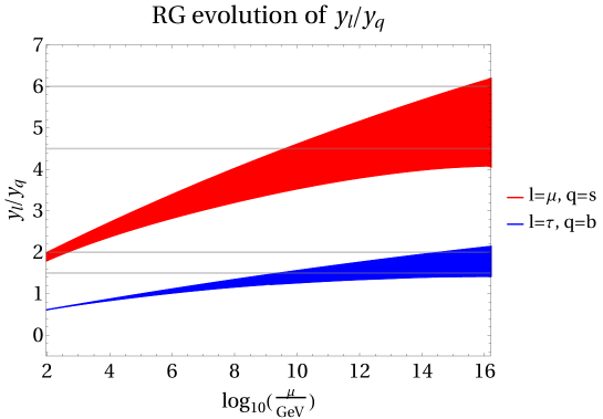
Figure 1: Estimated RG evolution of the 1-$\sigma$ ranges of the Yukawa ratios $y_{\tau}/y_{b}$ (blue) and $y_{\mu}/y_{s}$ (red) taking into account the effect of $Y_{1}$, $Y_{3}$ and $Y_{6}$. The horizontal grid lines indicate the values $\frac{3}{2}$, 2, $\frac{9}{2}$ and 6.

2.3 Toy models

After having argued that there are two viable possibilities for GUT scale charged lepton and down-type quark Yukawa ratios for the second and third generation, namely (i) $\frac{y_{\tau}}{y_{b}}=\frac{3}{2}$ and $\frac{y_{\mu}}{y_{s}}=\frac{9}{2}$, and (ii) $\frac{y_{\tau}}{y_{b}}=2$ and $\frac{y_{\mu}}{y_{s}}=6$, we now extend the two scenarios to “toy models” which also include the first family. Assuming the concept of single operator dominance, Table I shows which operator is dominant in which entry of the Yukawa matrices $Y_{\bm{\overline{5}}}$, $Y_{\bm{10}}$, and $Y_{\Delta}$ which were defined in Section 2.2.1.

operator	model 1	model 2
$(Y_{\Delta})_{ij}$	${\bm{\overline{5}_{F}}}_{i}{\bm{\overline{5}_{F}}}_{j}\bm{15_{H}}$	${\bm{\overline{5}_{F}}}_{i}{\bm{\overline{5}_{F}}}_{j}\bm{15_{H}}$
$(Y_{\bm{10}})_{ij}$	${\bm{10_{F}}}_{i}{\bm{10_{F}}}_{j}{\bm{5_{H}}}$	${\bm{10_{F}}}_{i}{\bm{10_{F}}}_{j}{\bm{5_{H}}}$
$(Y_{\bm{\overline{5}}})_{11}$	$({\bm{10_{F}}}_{1}\bm{5_{H}}^{*})_{\bm{5}}(\bm{24_{H}})_{\bm{24}}(\bm{1_{H}})(\bm{24_{H}})_{\bm{24}}({\bm{\overline{5}_{F}}}_{1}\bm{1_{H}})_{\bm{\overline{5}}}$	$({\bm{10_{F}}}_{1}\bm{45_{H}}^{*})_{\bm{\overline{45}}}({\bm{\overline{5}_{F}}}_{1}\bm{24_{H}})_{\bm{45}}$
$(Y_{\bm{\overline{5}}})_{22}$	$({\bm{10_{F}}}_{2}{\bm{45_{H}}^{*}})_{\bm{5}}({\bm{\overline{5}_{F}}}_{2}\bm{24_{H}})_{\bm{\overline{5}}}$	$({\bm{10_{F}}}_{2}{\bm{24_{H}}})_{\bm{10}}({\bm{\overline{5}_{F}}}_{2}\bm{5_{H}})_{\bm{\overline{10}}}$
$(Y_{\bm{\overline{5}}})_{33}$	$({\bm{10_{F}}}_{3}{\bm{5_{H}}^{*}})_{\bm{45}}({\bm{\overline{5}_{F}}}_{3}\bm{24_{H}})_{\bm{\overline{45}}}$	$({\bm{10_{F}}}_{3}{\bm{45_{H}}^{*}})_{\bm{5}}(\bm{24_{H}})_{\bm{24}}({\bm{\overline{5}_{F}}}_{3}\bm{1_{H}})_{\bm{\overline{5}}}$

Table I: Dominant operators in the respective Yukawa entries in the two toy models.

From the renormalizable operator ${\bm{\overline{5}_{F}}}{\bm{\overline{5}_{F}}}\bm{15_{H}}$ we get the GUT scale relation

$$Y_{1}=Y_{3}=Y_{6}.$$ (2.26)

Moreover, since $Y_{\bm{10}}$ is dominated by the operator ${\bm{10_{F}}}{\bm{10_{F}}}{\bm{5_{H}}}$, the up-type Yukawa matrix is symmetric, i.e. $Y_{u}=Y_{u}^{T}$. We assume that the operator ${\bm{10_{F}}}{\bm{10_{F}}}{\bm{45_{H}}}$, which would yield anti-symmetric contributions, vanishes as a consequence of an appropriate family symmetry (see e.g. Antusch:2021yqe for an example of such a symmetry). Furthermore, at the GUT scale the Yukawa matrices $Y_{e}$ and $Y_{d}$ are in the two “toy models” related via Antusch:2009gu ; Antusch:2013rxa

$$\text{model 1:}\qquad Y_{e}=\text{diag}\left(\frac{4}{9},\frac{9}{2},\frac{3}{2}\right)\cdot Y_{d}^{T},$$ (2.27)

$$\text{model 2:}\qquad Y_{e}=\text{diag}\left(\frac{1}{2},6,2\right)\cdot Y_{d}^{T}.$$ (2.28)

3 Numerical analysis

3.1 Implementation

The models 1 and 2 defined in Section 2.3 are implemented at the GUT scale. Since they only differ in their corresponding charged lepton sector, all other sectors can be implemented identically in both of the two “toy models”. The symmetric Yukawa matrices $Y_{u}$ and $Y_{\Delta}$ can be diagonalized by a Takagi decomposition:

$$Y_{u} =U_{u}^{\dagger}Y_{u}^{\text{diag}}U_{u}^{*},$$ (3.29)

$$Y_{\Delta} =U_{\Delta}Y_{\Delta}^{\text{diag}}U_{\Delta}^{T},$$ (3.30)

where $U_{u}$ and $U_{\Delta}$ are unitary matrices and $Y_{u}^{\text{diag}}$ as well as $Y_{\Delta}^{\text{diag}}$ are defined as

$$Y_{u}^{\text{diag}} =\text{diag}(y_{1}^{u},y_{2}^{u},y_{3}^{u}),$$ (3.31)

$$Y_{\Delta}^{\text{diag}} =\text{diag}(y_{1}^{\Delta},y_{2}^{\Delta},y_{3}^{\Delta}),$$ (3.32)

with $y_{i}^{u}$ and $y_{i}^{\Delta}$ being real entries larger or equal to zero for $i=1,2,3.$ The unitary matrices $U_{g}$ ($g=u,\Delta$) can be parametrized by the physical parameters $\theta_{12}^{g}$, $\theta_{13}^{g}$, $\theta_{23}^{g}$, $\delta^{g}$, $\beta_{1}^{g}$, and $\beta_{2}^{g}$ as well as the unphysical parameters $\alpha_{1}^{g}$, $\alpha_{2}^{g}$, and $\alpha_{3}^{g}$. The latter will be set to zero for the analysis. The matrices $U_{g}$ then read

$$U_{g}=\begin{pmatrix}e^{i\alpha_{1}^{g}}&0&0\\ 0&e^{i\alpha_{2}^{g}}&0\\ 0&0&e^{i\alpha_{3}^{g}}\end{pmatrix}\begin{pmatrix}1&0&0\\ 0&c_{23}^{g}&s_{23}^{g}\\ 0&-s_{23}^{g}&c_{23}^{g}\end{pmatrix}\begin{pmatrix}c_{13}^{g}&0&s_{13}^{g}e^{-i\delta^{g}}\\ 0&1&0\\ -s_{13}^{g}e^{i\delta^{g}}&0&c_{13}^{g}\end{pmatrix}\begin{pmatrix}c_{12}^{g}&s_{12}^{g}&0\\ -s_{12}^{g}&c_{12}^{g}&0\\ 0&0&1\end{pmatrix}\begin{pmatrix}e^{i\beta_{1}^{g}}&0&0\\ 0&e^{i\beta_{2}^{g}}&0\\ 0&0&1\end{pmatrix},$$ (3.33)

where $s_{ij}^{g}=\sin(\theta_{ij}^{g})$, $c_{ij}^{g}=\cos(\theta_{ij}^{g})$, $i,j=1,2,3$. Then the matrices $Y_{1}$, $Y_{3}$ and $Y_{6}$ are given by the relation

$$Y_{1}=Y_{3}=Y_{6}=Y_{\Delta}.$$ (3.34)

The down-type Yukawa matrix $Y_{d}$ is implemented as a diagonal matrix with real positive entries

$$Y_{d}=\text{diag}(y_{1}^{d},y_{2}^{d},y_{3}^{d}).$$ (3.35)

The charged lepton Yukawa matrix is for the two models then given by Eq. (2.27) and Eq. (2.28), respectively, and implemented accordingly.

3.2 Parameters and observables

After having discussed the implementation of the Yukawa matrices, we now give the GUT scale input parameters. In total, there are 36 parameters, some of which can be ignored for some parts of the numerical analysis (cf. Section 3.3). These parameters decompose into the GUT scale $M_{\text{GUT}}$, the unified gauge coupling $g_{\text{GUT}}$, the intermediate-scale masses $m_{\Delta_{1}},$ $m_{\Delta_{3}},$ $m_{\Delta_{6}},$ $m_{\phi_{1}},$ $m_{\phi_{2}},$ $m_{\phi_{3}},$ $m_{\phi_{4}},$ $m_{\phi_{5}},$ $m_{t_{1}},$ $m_{t_{2}},$ $m_{\Sigma_{1}},$ $m_{\Sigma_{8}}$, the scalar coupling constant $\mu$, the singular values $y_{1}^{u},$ $y_{2}^{u},$ $y_{3}^{u},$ $y_{1}^{d},$ $y_{2}^{d},$ $y_{3}^{d},$ $y_{1}^{\Delta},$ $y_{2}^{\Delta},$ $y_{3}^{\Delta}$ as well as the angles $\theta_{12}^{u},$ $\theta_{13}^{u},$ $\theta_{23}^{u},$ $\theta_{12}^{\Delta},$ $\theta_{13}^{\Delta},$ $\theta_{23}^{\Delta}$ and phases $\delta^{u},$ $\beta_{1}^{u},$ $\beta_{2}^{u},$ $\delta^{\Delta},$ $\beta_{1}^{\Delta},$ $\beta_{2}^{\Delta}$ of the Yukawa matrices. The following list summarizes all the input parameters as well as their allowed ranges:

$$M_{\text{GUT}} <M_{Pl},$$

$$m_{\Delta_{1}},m_{\Delta_{3}},m_{\Delta_{6}},m_{\phi_{1}},m_{\phi_{2}},m_{\phi_{3}},m_{\phi_{4}},m_{\phi_{5}},m_{\Sigma_{1}},m_{\Sigma_{8}} \in[500\,\text{GeV},M_{\text{GUT}}],$$

$$m_{t_{1}},m_{t_{2}} \in[10^{11}\,\text{GeV},M_{\text{GUT}}],$$

$$\mu <3m_{\Delta_{1}},$$

$$g_{\text{GUT}},\,y_{1}^{u},\,y_{2}^{u},\,y_{3}^{u},\,y_{1}^{d},\,y_{2}^{d},\,y_{3}^{d} \in[0,1],$$ (3.36)

$$y_{1}^{\Delta},\,y_{2}^{\Delta},\,y_{3}^{\Delta} \in[0,1.9],$$

$$\theta_{12}^{u},\,\theta_{13}^{u},\,\theta_{23}^{u},\,\theta_{12}^{\Delta},\,\theta_{13}^{\Delta},\,\theta_{23}^{\Delta} \in[0,\pi/2],$$

$$\delta^{u},\,\beta_{1}^{u},\,\beta_{2}^{u},\,\delta^{\Delta},\,\beta_{1}^{\Delta},\,\beta_{2}^{\Delta} \in[-\pi,\pi).$$

The two models are fitted to the following 22 low energy observables (as well as to the nucleon decay rates for 13 different decay channels, see Table II):

$$g_{1},\,g_{2},\,g_{3}$$

$$y_{u},\,y_{c},\,y_{t},\,y_{d},\,y_{s},\,y_{b},\,\theta_{12}^{\text{CKM}},\,\theta_{13}^{\text{CKM}},\,\theta_{23}^{\text{CKM}},\,\delta^{\text{CKM}},\,y_{e},\,y_{\mu},\,y_{\tau},\,\hskip 17.07182pt$$ (3.37)

$$\Delta m_{21}^{2},\,\Delta m_{31}^{2},\,\theta_{12}^{\text{PMNS}},\,\theta_{13}^{\text{PMNS}},\,\theta_{23}^{\text{PMNS}},\,\delta^{\text{PMNS}}.$$

The GUT scale $M_{\text{GUT}}$, the unified gauge coupling $g_{\text{GUT}}$ as well as the intermediate-scale masses are used to fit the SM gauge couplings $g_{1}$, $g_{2}$ and $g_{3}$. Moreover, since the quasi-Yukawa couplings $Y_{1}$, $Y_{3}$ and $Y_{6}$ effect the RG evolution of the SM Yukawa couplings $Y_{e}$ and $Y_{d}$, the masses $m_{\Delta_{1}}$, $m_{\Delta_{3}}$ and $m_{\Delta_{6}}$ are further used to fit the singular values of the charged-lepton Yukawa matrix $y_{e}$, $y_{\mu}$ and $y_{\tau}$. The singular values $y_{i}^{u}$ and $y_{i}^{d}$ ($i=1,2,3$) are used to fit the up- and down-type Yukawa couplings, while the angles $\theta_{12}^{u}$, $\theta_{13}^{u}$, $\theta_{23}^{u}$, and the phase $\delta^{u}$ are used to fit the CKM parameters. The singular values $y_{i}^{\Delta}$ ($i=1,2,3$) together with the trilinear coupling $\mu$ as well as the angles $\theta_{12}^{\Delta}$, $\theta_{13}^{\Delta}$, $\theta_{23}^{\Delta}$, $\delta^{\Delta}$ are used to fit the neutrino sector. Furthermore, the phases $\beta_{1}^{\Delta}$ and $\beta_{2}^{\Delta}$ are related to the Majorana phases in the PMNS matrix. Finally, the phases $\beta_{1}^{u}$ and $\beta_{2}^{u}$ are the so-called GUT phases Ellis:1979hy ; Ellis:2019fwf . They have an impact on the nucleon decay rates, but do not change the predictions for the SM parameters.

	decay channel	$\tau/\mathcal{B}$ [year]	$\Gamma_{\text{partial}}$ [GeV]
Proton:	$p\rightarrow\pi^{0}\,e^{+}$	$>\,2.4\cdot 10^{34}$	$>\,8.7\cdot 10^{-67}$
	$p\rightarrow\pi^{0}\,\mu^{+}$	$>\,1.6\cdot 10^{34}$	$>\,1.3\cdot 10^{-66}$
	$p\rightarrow\eta^{0}\,e^{+}$	$>\,4.1\cdot 10^{33}$	$>\,5.1\cdot 10^{-66}$
	$p\rightarrow\eta^{0}\,\mu^{+}$	$>\,1.2\cdot 10^{33}$	$>\,1.7\cdot 10^{-65}$
	$p\rightarrow K^{0}\,e^{+}$	$>\,1.1\cdot 10^{33}$	$>\,1.9\cdot 10^{-65}$
	$p\rightarrow K^{0}\,\mu^{+}$	$>\,1.6\cdot 10^{34}$	$>\,1.3\cdot 10^{-66}$
	$p\rightarrow\pi^{+}\,\overline{\nu}$	$>\,2.8\cdot 10^{32}$	$>\,7.4\cdot 10^{-65}$
	$p\rightarrow K^{+}\,\overline{\nu}$	$>\,6.6\cdot 10^{33}$	$>\,3.2\cdot 10^{-66}$
Neutron:	$n\rightarrow\pi^{-}\,e^{+}$	$>\,2.1\cdot 10^{33}$	$>\,1.0\cdot 10^{-65}$
	$n\rightarrow\pi^{-}\,\mu^{+}$	$>\,9.9\cdot 10^{32}$	$>\,2.1\cdot 10^{-65}$
	$n\rightarrow\pi^{0}\,\overline{\nu}$	$>\,9.9\cdot 10^{32}$	$>\,2.1\cdot 10^{-65}$
	$n\rightarrow\eta^{0}\,\overline{\nu}$	$>\,5.6\cdot 10^{32}$	$>\,3.7\cdot 10^{-65}$
	$n\rightarrow K^{0}\,\overline{\nu}$	$>\,1.2\cdot 10^{32}$	$>\,1.7\cdot 10^{-64}$

Table II: Current experimental bounds Dev:2022jbf on the decay widths $\Gamma_{\text{partial}}$ (respectively lifetime bound $\tau/\mathcal{B}$, where $\mathcal{B}$ is the branching ratio for the decay channel) for various nucleon decay channels at 90 % confidence level. The data stems from Figure 5-3 of Brock:2012ogj and was updated with the findings from Mine:2016mxy ; Takenaka:2020vqy ; Bajc:2016qcc ; Miura:2016krn ; Abe:2014mwa ; 1205.6538 .

3.3 Fit to experimental data

As described in Section 3.1 we implement the input parameters given in Eq. (3.2) at the GUT scale $M_{\text{GUT}}$ and compute the running to the $Z$ scale $M_{Z}$. The running of the SM gauge couplings is computed at 2-loop, while the running of the (quasi-) Yukawa matrices as well as the effective neutrino mass operators is accounted for at 1-loop. Then, at $M_{Z}$ the singular values of the SM Yukawa matrices as well as the CKM and PMNS parameters and the neutrino squared mass differences are determined. Furthermore, as described in Antusch:2021yqe , the nucleon decay widths for the 13 different decay channels listed in Table II are computed, using the Mathematica package ProtonDecay Antusch:2020ztu for the final step of this computation.

At the low scale $M_{Z}$ we define the total $\chi^{2}$-function by the sum of the pulls $\chi_{i}^{2}$ for each observable $i$

$$\chi^{2}(\vec{x})=\sum_{i}\chi_{i}^{2}(\vec{x}),$$ (3.38)

where $\vec{x}$ represents a vector which consists of the input parameters listed in Eq. (3.2). While we use the exact pull $\chi_{i}^{2}$ given by NuFIT 5.1 Esteban:2020cvm for the observables $\theta_{23}^{\text{PMNS}}$ and $\delta^{\text{PMNS}}$, we compute the pull $\chi_{i}^{2}$ for all other observables as

$$\chi_{i}^{2}(\vec{x})=\left(\frac{f_{i}(\vec{x})-y_{i}}{\sigma_{i}}\right)^{2},$$ (3.39)

where $f_{i}(\vec{x})$ is our prediction for the observable $i$, while $y_{i}$ represents the experimental central value and $\sigma_{i}$ its corresponding standard deviation. Using a differential evolution algorithm the $\chi^{2}$-function is minimized delivering a benchmark point. Afterwards, starting from that benchmark point, an MCMC analysis is performed using an adaptive Metropolis-Hastings algorithm Metropolis-Hastings-algorithm . For both models 16 independent chains with $2.5\times 10^{5}$ data points are computed with a flat prior probability distribution. Using these data points the posterior densities of various observables are calculated.

To simplify the analysis we do not vary all the input parameters listed in Eq. (3.2) for the minimization procedure. Keeping the masses $m_{\phi_{2}},$ $m_{\phi_{4}},$ $m_{\phi_{5}},$ $m_{t_{1}},$ $m_{t_{2}},$ $m_{\Sigma_{1}}$ and $m_{\Sigma_{8}}$ at the GUT scale still leaves enough freedom to fit the gauge couplings. Moreover, the correct neutrino mass squared differences can still be obtained if $y_{1}^{\Delta}$ is set to zero, which then implies a strong normal hierarchy of the light neutrino masses. Furthermore, since the CKM parameters are almost constant during the RG evolution, the parameters $\theta_{12}^{u}$, $\theta_{13}^{u}$, $\theta_{23}^{u}$, $\delta^{u}$ are not varied (and the observables $\theta_{12}^{\text{CKM}}$, $\theta_{13}^{\text{CKM}}$, $\theta_{23}^{\text{CKM}}$, $\delta^{\text{CKM}}$ are not considered in the $\chi^{2}$-function). Since the GUT phases $\beta_{1}^{u}$ and $\beta_{2}^{u}$ do not change the predictions for the SM parameters and usually only have a small effect on the nucleon decay predictions in non-SUSY models (see e.g. Antusch:2021yqe ) they can be set to zero. Finally, the Majorana phases are also set to zero since they only have a small effect on the running of the SM parameters. In summary, for the fitting procedure the following 20 input parameters are varied

$$M_{\text{GUT}},g_{\text{GUT}},m_{\Delta_{1}},m_{\Delta_{3}},m_{\Delta_{6}},m_{\phi_{1}},m_{\phi_{3}},\mu,$$

$$y_{1}^{u},\,y_{2}^{u},\,y_{3}^{u},\,y_{1}^{d},\,y_{2}^{d},\,y_{3}^{d},y_{2}^{\Delta},\,y_{3}^{\Delta},\theta_{12}^{\Delta},\,\theta_{13}^{\Delta},\,\theta_{23}^{\Delta},\delta^{\Delta},$$ (3.40)

giving a benchmark point. From this benchmark point the MCMC analysis — for which, on the other hand, all 36 input parameters are varied — is started.

4 Results

In this section we present our numerical results for the minimization of the $\chi^{2}$-function as well as for the MCMC analysis. We are interested in the predictions for the low-scale charged lepton and down-type quark Yukawa ratios which give a direct hint on the viability of the GUT scale Yukawa ratios. Furthermore, we give the predictions of the highest posterior densities (HPD) for the masses of the added scalar fields as well as the nucleon decay widths. All of these predictions may be used to test our models by upcoming experiments.

4.1 Benchmark points

Minimizing the $\chi^{2}$-function under the constraints presented in Section 3.3 gives for both models a benchmark point. The GUT scale input parameters for the benchmark points of both models are listed in Table III, while Table IV shows the respective total $\chi^{2}$ as well as the dominant pulls $\chi_{i}^{2}$. With a total $\chi^{2}$ of 1.86 model 2 gives a better fit than model 1 ($\chi^{2}=4.35$). In both models the dominant pull comes from the Yukawa coupling of the strange quark with $\chi_{y_{s}}^{2}=1.55\,(2.75)$ in model 2 (1).

Regarding the GUT scale input parameters, the main difference between the two models are the choices of the masses of the intermediate-scale scalar fields. The reason for this is that — as discussed in Section 2.2.3 — if $m_{\Delta_{1}}$ is well below the GUT scale, while $m_{\Delta_{6}}$ is close to the GUT scale the running of $Y_{e}$ is “speeded up” yielding larger charged lepton and down-type quark GUT scale ratios, while conversely, if $m_{\Delta_{6}}$ is well below the GUT scale, while $m_{\Delta_{1}}$ is close to the GUT scale the running of $Y_{d}$ is “speeded up” resulting in smaller charged lepton and down-type quark GUT scale ratios. This fixes the masses $m_{\Delta_{1}}$, $m_{\Delta_{3}}$ and $m_{\Delta_{6}}$ in the two models. The remaining masses have then to be chosen such that the gauge couplings can unify which is the reason why they differ in the two models.

Moreover, an interesting difference between the two models is the chosen GUT scale value for $\theta_{23}^{\Delta}$ which is, apart from renormalization group effects, equal to the observable $\theta_{23}^{\text{PMNS}}$. The current experimental 1-$\sigma$ range of this observable consists of two disjoint intervals. The benchmark point of model 1 predicts $\theta_{23}^{\text{PMNS}}$ to lie in the lower interval, while the benchmark point of model 2 suggests that $\theta_{23}^{\text{PMNS}}$ should lie in the upper interval. Therefore, a more precise measurement of $\theta_{23}^{\text{PMNS}}$ could distinguish between the two models (cf. Section 4.2).

		Model 1			Model 2
$g_{\text{GUT}}\;/\;10^{-1}$		6.12			6.39
$\log_{10}(M_{\text{GUT}}\;/\;\text{GeV})$		15.7			15.8
$\log_{10}(m_{\Delta_{1}}\;/\;\text{GeV})$		15.1			9.52
$\log_{10}(m_{\Delta_{3}}\;/\;\text{GeV})$		10.4			15.0
$\log_{10}(m_{\Delta_{6}}\;/\;\text{GeV})$		5.79			13.1
$\log_{10}(m_{\phi_{1}}\;/\;\text{GeV})$		9.97			2.70
$\log_{10}(m_{\phi_{3}}\;/\;\text{GeV})$		6.72			9.56
$\log_{10}(\mu\;/\;\text{GeV})$		15.6			4.34
$y_{1}^{u}\;/\;10^{-6}$		2.69			2.24
$y_{2}^{u}\;/\;10^{-3}$		1.31			1.10
$y_{3}^{u}\;/\;10^{-1}$		4.05			3.35
$y_{1}^{d}\;/\;10^{-6}$		6.03			5.11
$y_{2}^{d}\;/\;10^{-4}$		1.39			0.96
$y_{3}^{d}\;/\;10^{-3}$		7.48			4.82
$y_{2}^{\Delta}\;/\;10^{-1}$		1.92			1.28
$y_{3}^{\Delta}\;/\;10^{-1}$		19.0			9.46
$\theta^{\Delta}_{12}\;/\;10^{-1}$		5.81			5.82
$\theta^{\Delta}_{13}\;/\;10^{-1}$		1.15			1.33
$\theta^{\Delta}_{23}\;/\;10^{-1}$		6.00			8.00
$\delta^{\Delta}$		3.39			3.39

Table III: The GUT scale input parameters of the benchmark points for both models.

	$\chi^{2}$	$\chi^{2}_{y_{s}}$	$\chi^{2}_{y_{b}}$	$\chi^{2}_{y_{\mu}}$	$\chi^{2}_{y_{\tau}}$	$\chi^{2}_{\theta_{23}^{\text{PMNS}}}$	$\chi^{2}_{\Gamma({p\rightarrow\pi^{0}e^{+}})}$
model 1	4.35	2.75	0.23	0.09	0.23	0.72	0.21
model 2	1.86	1.55	0.09	0.05	0.09	0.00	0.03

Table IV: The total $\chi^{2}$ as well as the dominant pulls $\chi_{i}^{2}$ for the benchmark points of both models.

4.2 MCMC analysis

We obtain the highest posterior densities of different quantities using an MCMC analysis varying the input parameters around the benchmark points. For this analysis all the input parameters listed in Eq. (3.2) are varied.

1. Charged lepton and down-type quark Yukawa ratios
   Figure 2 shows the 1-$\sigma$ (dark) and 2-$\sigma$ (light) HPD intervals of the charged lepton and down-type quark Yukawa ratios at the low scale $M_{Z}$ for model 1 (red) and model 2 (green). The experimental 1-$\sigma$ range is indicated by the white region, while the dashed line represents the current experimental central value. As it could already be seen from the benchmark points (cf. Section 4.1), the ratio $\frac{y_{\mu}}{y_{s}}$ is predicted to be above the experimental central value in both models. However, there is an intersection between the 1-$\sigma$ HPD interval and the experimentally allowed 1-$\sigma$ region. Future experimental measurements of the three ratios can further test the two models.

   

   

   

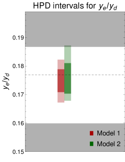
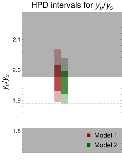
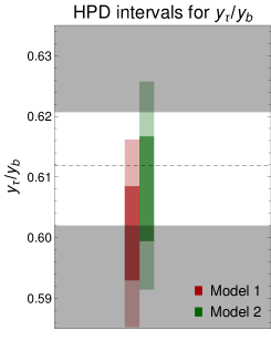
   Figure 2: The predicted 1-$\sigma$ and 2-$\sigma$ HPD intervals of the charged lepton and down-type quark Yukawa ratios at $M_{Z}.$

2. PMNS mixing angle $\theta_{23}^{\text{PMNS}}$
   As it was pointed out in Section 4.1 the benchmark points indicate distinct predictions for the observable $\theta_{23}^{\text{PMNS}}$. Figure 3 shows that the predicted HPD intervals for model 1 lie within the lower experimentally allowed region, while the predicted HPD intervals of model 2 span over both allowed regions. Therefore, a measurement of $\theta_{23}^{\text{PMNS}}$ in the upper interval would favor model 2 over model 1.

   

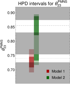
   Figure 3: The predicted 1-$\sigma$ and 2-$\sigma$ HPD intervals at $M_{Z}$ of the PMNS mixing angle $\theta_{23}^{\text{PMNS}}$.

3. Intermediate-scale scalar masses
   The prediction for the 1-$\sigma$ and 2-$\sigma$ HPD intervals of the masses of the added scalar fields are presented in Figure 6. The ranges for most of the masses are quite large. However, some of the fields could be observed by future experiments. Especially interesting is the predicted range of $m_{\phi_{1}}$ in model 2. The upper bound of the predicted 1-$\sigma$ and 2-$\sigma$ HPD interval is given by 13.5 TeV and 207 TeV, respectively. Moreover, a possible observation of one of the fields $\Delta_{6}$, $\phi_{1}$ or $\phi_{3}$ could distinguish between the two models.

4. Nucleon decay widths
   Figure 6 visualizes the predicted 1-$\sigma$ and 2-$\sigma$ HPD intervals for the nucleon decay widths of various decay channels (cf. Table II). The horizontal blue lines indicate the current experimental bound at a 90 % confidence level. For the dominant decay channel, $p\rightarrow\pi^{0}e^{+}$, also the expected bounds of the planned DUNE Acciarri:2015uup and Hyper-Kamiokande experiment Abe:2018uyc are shown. Of particular interest will be the planned Hyper-Kamiokande experiment which will test the full 1-$\sigma$ region of this decay channel predicted by model 1.

   Moreover, as Figure 4 shows, model 1 predicts a lower GUT scale than model 2. Therefore, model 1 generally predicts larger decay widths than model 2. The 1-$\sigma$ HPD intervals do not intersect for any of the decay channels. This fact can be used to distinguish between the two models if nucleon decay is observed in at least one of the 13 different decay channels. However, as it was pointed out in Antusch:2021yqe the Yukawa texture has a non-trivial effect on the nucleon decay predictions. This means that if different Yukawa textures were considered (which still predict the GUT scale relations $\frac{y_{\tau}}{y_{b}}=\frac{3}{2}$ and $\frac{y_{\mu}}{y_{s}}=\frac{9}{2}$, respectively $\frac{y_{\tau}}{y_{b}}=2$ and $\frac{y_{\mu}}{y_{s}}=6$) the two scenarios might no-longer be distinguished so easily.

   

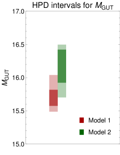
   Figure 4: Predicted 1-$\sigma$ and 2-$\sigma$ HPD intervals of the GUT scale $M_{\text{GUT}}$ for both models.

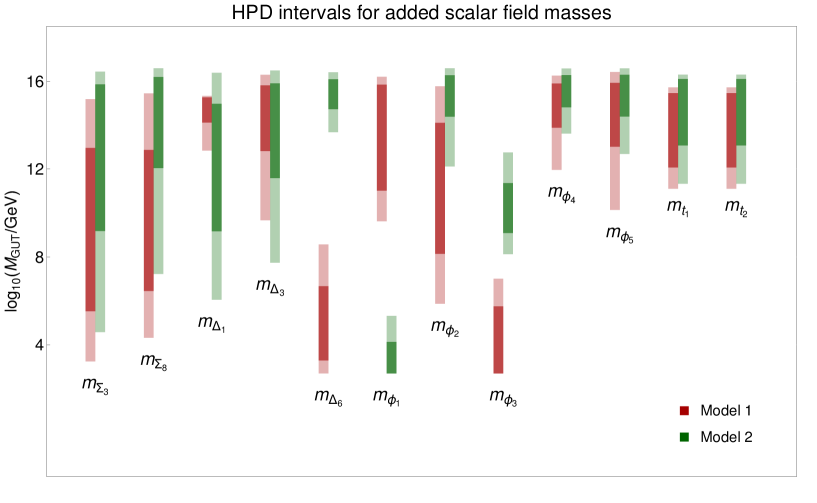
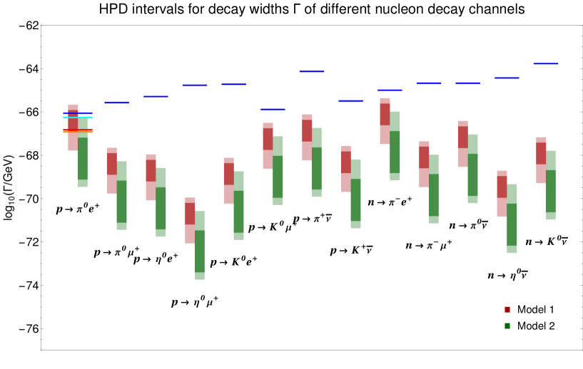
Figure 5: The predicted 1-$\sigma$ and 2-$\sigma$ HPD intervals of the intermediate-scale scalar masses.

Figure 6: The predicted 1-$\sigma$ and 2-$\sigma$ HPD intervals of the decay widths for various different nucleon decay channels. The current experimental bounds at 90 % confident level are indicated by blue lines (cf. Table II). Moreover, the future sensitivity of DUNE Acciarri:2015uup for the decay channel $p\rightarrow\pi^{0}e^{+}$ is represented by a cyan line, while the future sensitivity of Hyper-Kamiokande Abe:2018uyc with one tank (two tanks) for this decay channel is indicated by a red (orange) line.

It is interesting to note that part of the parameter space, as depicted in Fig. 6, is already ruled out by existing collider searches. In the following, we briefly summarize the current collider limits.

The color-octet scalar $\phi_{1}$ has both neutral $\phi_{1}^{0}$ and charged $\phi_{1}^{+}$ components. The charged partner provides a stronger bound since it cannot decay to gluons. These states can be efficiently produced via gluon-fusion $pp\to\phi_{1}^{+}\phi_{1}^{-},\overline{t}b\phi_{1}^{+}$ at the LHC, which lead to $pp\to\overline{t}bt\overline{b}$. The analysis performed in Ref. Miralles:2019uzg shows that the current LHC data provides a lower bound of $m_{\phi_{1}^{+}}>800$ GeV. The neutral components can also be pair-produced through gluon-fusion, and for our scenario, this would lead to $pp\to\overline{b}b\overline{b}b$. LHC currently provides a lower bound Hayreter:2017wra on its mass of $m_{\phi_{1}^{0}}>530$ GeV, which is weaker than its charged partner.

Concerning the scalar leptoquark $\phi_{3}$, which couples predominantly to the second (third) generation quark-lepton pairs for model-1 (model-2), current LHC data limits its mass to be greater than $\gtrsim 1.7$ TeV ATLAS:2020dsk ($\gtrsim 1.4$ TeV ATLAS:2019qpq ; ATLAS:2021oiz ) from pair-produced leptoquarks decaying into $jj\mu\overline{\mu}$ (or $bb\tau\overline{\tau}$) final state.

For both models, the sextet diquark $\Delta_{6}$ that couples to right-handed down-type quarks $d_{Ri}d_{Rj}$, has Yukawa coupling of the form $\sim U_{\textrm{PMNS}}\;\textrm{diag}\{0,\mathcal{O}(0.1),\mathcal{O}(1)\}\;U^{T}_{\textrm{PMNS}}$. Subsequently, the coupling to $d_{R}d_{R}$ is somewhat small; however, due to $\mathcal{O}(0.1)$ couplings with $d_{R}s_{R}$ and $s_{R}s_{R}$, it can still be produced through the annihilation of a pair of quarks via an $s$-channel resonance. By considering equal diquark couplings of electromagnetic strength $y_{12,13,23}\sim 0.3$, and using the CMS measurements of narrow dijet resonances at $\sqrt{13}$ TeV CMS:2018mgb , a lower bound on its mass $\gtrsim 2.5$ TeV is obtained in Ref. Pascual-Dias:2020hxo . This bound is expected to get relaxed in our scenario due to additional non-zero diagonal couplings and the somewhat smaller Yukawa couplings involved in the production. On the other hand, a search for pair-produced resonances in four-jet final states finds diquark mass $\gtrsim 610$ GeV if the decay is into a $b$-quark and a light-quark ATLAS:2017jnp . To obtain the exact bound, however, a dedicated collider study would be required.

Future LHC upgrades have the potential to discover some of these colored particles that could be used to distinguish between these two models.

5 Conclusions

In this work we considered a rather minimal $SU(5)$ GUT scenario which contains a 45-dimensional as well as a 15-dimensional Higgs representation on top of the Georgi-Glashow $SU(5)$ particle content and in which neutrino masses are generated by a type II seesaw mechanism. We showed that within the concept of single operator dominance in the third and second family this scenario can lead to two different GUT scale predictions for charged lepton and down-type Yukawa ratios, namely (i) $\frac{y_{\tau}}{y_{b}}=\frac{3}{2}$ and $\frac{y_{\mu}}{y_{s}}=\frac{9}{2}$, respectively (ii) $\frac{y_{\tau}}{y_{b}}=2$ and $\frac{y_{\mu}}{y_{s}}=6$. We investigated the compatibility of both of these two combinations of GUT scale Yukawa ratios with the low-energy experimental data by computing the RG evolution and taking into account the contribution of new arising Yukawa interactions on the beta functions of the charged lepton and down-type quark Yukawa matrices (cf. Figure 1). The outcome of this analysis motivated the formulation of two “toy models” which also contain the first family. We investigated various predictions of these “toy models” in Section 4 and showed that there are several possibilities to distinguish between them in future experiments, namely the nucleon decay rates, the masses of the fields $\Delta_{6}$, $\phi_{1}$ or $\phi_{3}$, which could be discovered at colliders, as well as the prediction for the PMNS 2-3 mixing angle $\theta_{23}^{\text{PMNS}}$.

Appendix A Renormalization group equations of gauge and Yukawa couplings

In the following we list the RGEs of the gauge and Yukawa couplings which we have obtained using the Mathematica package SARAH Staub:2008uz ; Staub:2013tta .

A.1 Gauge part

The 2-loop RGEs for gauge couplings ($i,k=1,2,3$) read

$$\mu\frac{dg_{i}}{d\mu}=g^{3}_{i}\bigg{\{}\frac{1}{16\pi^{2}}a_{i}+\frac{1}{(16\pi^{2})^{2}}\left(\sum_{k}b_{ik}g^{2}_{k}+\beta^{Y}_{i}\right)\bigg{\}},$$ (A.41)

where $a_{i}$ ($b_{ik}$) the 1-loop (2-loop) gauge coefficients and $\beta^{Y}_{i}$ denotes the 2-loop Yukawa contribution. They are given by

$$a_{i}=a^{SM}_{i}+\sum_{I}a^{I}_{i}\mathcal{H}(\mu,m_{I})\;,\qquad b_{ik}=b_{ik}^{SM}+\sum_{I}b_{ik}^{I}\mathcal{H}(\mu,m_{I})\;,$$ (A.42)

$$\beta_{i}^{Y}=\beta_{i}^{Y,SM}+\sum_{I}\beta_{i}^{Y,I}\mathcal{H}(\mu,m_{I})\;,$$

with $I$ denoting the respective particle and $\mathcal{H}$ the Heaviside step function which was defined in Eq. (2.25). The 1-loop coefficients read

$$a^{SM}_{i}=\left(\frac{41}{10},-\frac{19}{6},-7\right),\;\;a^{\Delta_{1}}_{i}=\left(\frac{3}{5},\frac{2}{3},0\right),\;\;a^{\Delta_{3}}_{i}=\left(\frac{1}{30},\frac{1}{2},\frac{1}{3}\right),$$

$$a^{\Delta_{6}}_{i}=\left(\frac{8}{15},0,\frac{5}{6}\right),\;\;a^{\phi_{1}}_{i}=\left(\frac{4}{5},\frac{4}{3},2\right),\;\;a^{\phi_{2}}_{i}=\left(\frac{2}{15},0,\frac{5}{6}\right),$$ (A.43)

$$a^{\phi_{3}}_{i}=\left(\frac{1}{5},2,\frac{1}{2}\right),\;\;a^{\phi_{4}}_{i}=\left(\frac{49}{30},\frac{1}{2},\frac{1}{3}\right),\;\;a^{\phi_{5}}_{i}=\left(\frac{1}{15},0,\frac{1}{6}\right),$$

$$a^{\phi_{6}}_{i}=\left(\frac{16}{15},0,\frac{1}{6}\right),\;\;a^{\Sigma_{3}}_{i}=\left(0,\frac{1}{3},0\right),\;\;a^{\Sigma_{8}}_{i}=\left(0,0,\frac{1}{2}\right),$$

while the 2-loop coefficients are given by

$$b^{SM}_{ik}=\begin{pmatrix}\frac{199}{50}&\frac{27}{10}&\frac{44}{5}\\ \frac{9}{10}&\frac{35}{6}&12\\ \frac{11}{10}&\frac{9}{2}&-26\end{pmatrix},\;\;b^{\Delta_{1}}_{ik}=\begin{pmatrix}\frac{108}{25}&\frac{72}{5}&0\\ \frac{24}{5}&\frac{56}{3}&0\\ 0&0&0\end{pmatrix},\;\;b^{\Delta_{3}}_{ik}=\begin{pmatrix}\frac{1}{150}&\frac{3}{10}&\frac{8}{15}\\ \frac{1}{10}&\frac{13}{2}&8\\ \frac{1}{15}&3&\frac{22}{3}\end{pmatrix},$$

$$b^{\Delta_{6}}_{ik}=\begin{pmatrix}\frac{128}{75}&0&\frac{64}{3}\\ 0&0&0\\ \frac{8}{3}&0&\frac{115}{3}\end{pmatrix},\;\;b_{ik}^{\phi_{1}}=\begin{pmatrix}\frac{36}{25}&\frac{36}{5}&\frac{144}{5}\\ \frac{12}{5}&\frac{52}{3}&48\\ \frac{18}{5}&18&84\end{pmatrix},\;\;b_{ik}^{\phi_{2}}=\begin{pmatrix}\frac{8}{75}&0&\frac{16}{3}\\ 0&0&0\\ \frac{2}{3}&0&\frac{115}{3}\end{pmatrix},$$ (A.44)

$$b_{ik}^{\phi_{3}}=\begin{pmatrix}\frac{4}{25}&\frac{24}{5}&\frac{16}{5}\\ \frac{8}{5}&56&32\\ \frac{2}{5}&12&11\end{pmatrix},\;\;b_{ik}^{\phi_{4}}=\begin{pmatrix}\frac{2401}{150}&\frac{147}{10}&\frac{392}{15}\\ \frac{49}{10}&\frac{13}{2}&8\\ \frac{49}{15}&3&\frac{22}{3}\end{pmatrix},\;\;b_{ik}^{\phi_{5}}=\begin{pmatrix}\frac{4}{75}&0&\frac{16}{15}\\ 0&0&0\\ \frac{2}{15}&0&\frac{11}{3}\end{pmatrix},$$

$$b_{ik}^{\phi_{6}}=\begin{pmatrix}\frac{1024}{75}&0&\frac{256}{15}\\ 0&0&0\\ \frac{32}{15}&0&\frac{11}{3}\end{pmatrix},\;\;b_{ik}^{\Sigma_{3}}=\begin{pmatrix}0&0&0\\ 0&\frac{28}{3}&0\\ 0&0&0\end{pmatrix},\;\;b_{ik}^{\Sigma_{8}}=\begin{pmatrix}0&0&0\\ 0&0&0\\ 0&0&21\end{pmatrix}.$$

For the 2-loop Yukawa contributions we obtain

$$\beta^{SM,Y}_{1}=-\frac{17}{10}Tr\left[Y_{u}Y_{u}^{\dagger}\right]-\frac{1}{2}Tr\left[Y_{d}Y_{d}^{\dagger}\right]-\frac{3}{2}Tr\left[Y_{e}Y_{e}^{\dagger}\right],$$

$$\beta^{SM,Y}_{2}=-\frac{3}{2}Tr\left[Y_{u}Y_{u}^{\dagger}\right]-\frac{3}{2}Tr\left[Y_{d}Y_{d}^{\dagger}\right]-\frac{1}{2}Tr\left[Y_{e}Y_{e}^{\dagger}\right],$$ (A.45)

$$\beta^{SM,Y}_{3}=-2Tr\left[Y_{u}Y_{u}^{\dagger}\right]-2Tr\left[Y_{d}Y_{d}^{\dagger}\right],$$

and

$$\bigg{\{}\beta_{1}^{Y,\Delta_{1}},\beta_{1}^{Y,\Delta_{3}},\beta_{1}^{Y,\Delta_{6}}\bigg{\}}=\bigg{\{}-\frac{9}{10}Tr\left[Y_{1}Y^{\ast}_{1}\right],-\frac{13}{10}Tr\left[Y_{3}Y^{\dagger}_{3}\right],-\frac{4}{5}Tr\left[Y_{6}Y^{\ast}_{6}\right]\bigg{\}},$$

$$\bigg{\{}\beta_{2}^{Y,\Delta_{1}},\beta_{2}^{Y,\Delta_{3}},\beta_{2}^{Y,\Delta_{6}}\bigg{\}}=\bigg{\{}-\frac{3}{2}Tr\left[Y_{1}Y^{\ast}_{1}\right],-\frac{3}{2}Tr\left[Y_{3}Y^{\dagger}_{3}\right],0\bigg{\}},$$ (A.46)

$$\bigg{\{}\beta_{3}^{Y,\Delta_{1}},\beta_{3}^{Y,\Delta_{3}},\beta_{3}^{Y,\Delta_{6}}\bigg{\}}=\bigg{\{}0,-Tr\left[Y_{3}Y^{\dagger}_{3}\right],-2Tr\left[Y_{6}Y^{\ast}_{6}\right]\bigg{\}}.$$

A.2 Yukawa part

The RGEs for Yukawa couplings ($a=u,d,e$) at 1-loop are of the form

$$\mu\frac{dY_{a}}{d\mu}=\frac{1}{16\pi^{2}}\bigg{\{}\beta^{SM}_{a}+\sum_{I}\beta^{I}_{a}\mathcal{H}(\mu,m_{I})\bigg{\}},$$ (A.47)

where $\beta_{a}^{SM}$ are the SM contributions and $\beta_{a}^{I}$ are the contributions coming from the new quasi-like Yukawa couplings $Y_{1}$, $Y_{3}$ and $Y_{6}$. The well-known SM contributions read Cheng:1973nv ; Machacek:1983fi

$$\beta^{SM}_{u}=Y_{u}\left(-\frac{17}{20}g^{2}_{1}-\frac{9}{4}g^{2}_{2}-8g^{2}_{3}+T\right)+Y_{u}\left(\frac{3}{2}Y^{\dagger}_{u}Y_{u}-\frac{3}{2}Y^{\dagger}_{d}Y_{d}\right),$$

$$\beta^{SM}_{d}=Y_{d}\left(-\frac{1}{4}g^{2}_{1}-\frac{9}{4}g^{2}_{2}-8g^{2}_{3}+T\right)+Y_{d}\left(-\frac{3}{2}Y^{\dagger}_{u}Y_{u}+\frac{3}{2}Y^{\dagger}_{d}Y_{d}\right),$$ (A.48)

$$\beta^{SM}_{e}=Y_{e}\left(-\frac{9}{4}g^{2}_{1}-\frac{9}{4}g^{2}_{2}+T\right)+Y_{e}\left(\frac{3}{2}Y^{\dagger}_{e}Y_{e}\right),$$

with $T=Tr\left[3Y^{\dagger}_{u}Y_{u}+3Y^{\dagger}_{d}Y_{d}+Y^{\dagger}_{e}Y_{e}\right]$. The contributions coming from the new couplings $Y_{1}$, $Y_{3}$ and $Y_{6}$ are

$$\beta^{\Delta_{1}}_{a}=\bigg{\{}0,\;0,\;Y_{e}\left(\frac{3}{2}Y^{\ast}_{1}Y_{1}\right)\bigg{\}},$$

$$\beta^{\Delta_{3}}_{a}=\bigg{\{}0,\;\left(Y_{3}Y^{\dagger}_{3}\right)Y_{d},\;Y_{e}\left(\frac{3}{2}Y^{\dagger}_{3}Y_{3}\right)\bigg{\}},$$ (A.49)

$$\beta^{\Delta_{6}}_{a}=\bigg{\{}0,\;\left(2Y_{6}Y^{\ast}_{6}\right)Y_{d},\;0\bigg{\}}.$$

Furthermore the RGEs of the quasi-like Yukawa couplings read (for $\alpha,\gamma=1,3,6$)

$$\mu\frac{dY_{\alpha}}{d\mu}=\frac{1}{16\pi^{2}}\bigg{\{}\beta_{\Delta_{\alpha}}+\sum_{\gamma\neq\alpha}\delta\beta^{\Delta_{\gamma}}_{\Delta_{\alpha}}\mathcal{H}(\mu,m_{\Delta_{\gamma}})\bigg{\}},$$ (A.50)

where we have defined $\beta_{\Delta_{\alpha}}$ by

$$\beta_{\Delta_{1}}=Y_{1}\left(-\frac{9}{10}g^{2}_{1}-\frac{9}{2}g^{2}_{2}+TrY_{1}Y^{\ast}_{1}\right)+Y_{1}\left(\frac{1}{2}Y^{\dagger}_{e}Y_{e}+3Y^{\ast}_{1}Y_{1}\right)+\left(\frac{1}{2}Y^{T}_{e}Y^{\ast}_{e}\right)Y_{1}\;,$$

$$\beta_{\Delta_{3}}=Y_{3}\left(-\frac{13}{10}g^{2}_{1}-\frac{9}{4}g^{2}_{2}-4g^{2}_{3}+TrY_{3}Y^{\dagger}_{3}\right)+Y_{3}\left(\frac{1}{2}Y^{\dagger}_{e}Y_{e}+\frac{5}{2}Y^{\dagger}_{3}Y_{3}\right)+\left(Y_{d}Y^{\dagger}_{d}\right)Y_{3}\;,$$

$$\beta_{\Delta_{6}}=Y_{6}\left(-\frac{2}{5}g^{2}_{1}-8g^{2}_{3}+TrY_{6}Y^{\ast}_{6}\right)+Y_{6}\left(Y^{\ast}_{d}Y_{d}^{T}+4Y^{\ast}_{6}Y_{6}\right)+\left(Y_{d}Y^{\dagger}_{d}\right)Y_{6}\;,$$ (A.51)

and $\beta_{\Delta_{\alpha}}^{\Delta_{\gamma}}$ as

$$\delta\beta_{\Delta_{1}}^{\Delta_{3}}=\frac{3}{2}Y_{1}Y^{\dagger}_{3}Y_{3}+\frac{3}{2}Y^{T}_{3}Y^{\ast}_{3}Y_{1}\;,\qquad\delta\beta_{\Delta_{1}}^{\Delta_{6}}=0\;,\qquad\delta\beta_{\Delta_{3}}^{\Delta_{1}}=\frac{3}{2}Y_{3}Y^{\ast}_{1}Y_{1}\;,$$

$$\delta\beta_{\Delta_{3}}^{\Delta_{6}}=2Y_{6}Y^{\ast}_{6}Y_{3}\;,\qquad\delta\beta_{\Delta_{6}}^{\Delta_{1}}=0\;,\qquad\delta\beta_{\Delta_{6}}^{\Delta_{3}}=Y_{3}Y^{\dagger}_{3}Y_{6}+Y_{6}Y^{\ast}_{3}Y^{T}_{3}\;.$$ (A.52)

Appendix B Renormalization group evolution of the neutrino mass operator

The RGE of the dimension five neutrino mass operator $\kappa$ is given by

$$\mu\frac{d\kappa}{d\mu}=\frac{1}{16\pi^{2}}\left\{\beta_{\kappa}^{SM}+\sum_{I=\Delta_{3},\Delta_{6}}\beta_{\kappa}^{I}\mathcal{H}(\mu,m_{I})\right\},$$ (B.53)

where the SM contribution $\beta_{\kappa}^{SM}$ is Antusch:2001ck

$$\beta_{\kappa}^{SM}=\kappa\left(-\frac{3}{2}Y_{e}^{\dagger}Y_{e}\right)+\left(-\frac{3}{2}Y_{e}^{T}Y_{e}^{*}\right)\kappa+\left(-\frac{3}{2}g_{2}^{2}+3T+\lambda\right)\kappa\;.$$ (B.54)

The neutrino mass operator $\kappa$ is obtained after the field $\Delta_{1}$ is integrated out below its mass scale $m_{\Delta_{1}}$ as described in Section 2.2.2. However, if the fields $\Delta_{3}$ and $\Delta_{6}$ have masses below $m_{\Delta_{1}}$, the quasi-like Yukawa couplings $Y_{3}$ and $Y_{6}$ potentially affect the running of $\kappa$. Considering all possible Feynman diagrams we have computed this contribution using the method described in Antusch:2001ck . We obtain $\beta_{\kappa}^{\Delta_{6}}=0$ and

$$\beta_{\kappa}^{\Delta_{3}}=\kappa\left(-\frac{3}{2}Y_{3}^{\dagger}Y_{3}\right)+\left(-\frac{3}{2}Y_{3}^{T}Y_{3}^{*}\right)\kappa\;.$$ (B.55)

Appendix C Perturbativity of $Y_{\Delta}$ above the GUT scale

As described in Section 2.2.3 the contribution of the quasi-like Yukawa matrices $Y_{1}$, $Y_{3}$ and $Y_{6}$ on the RG evolution of the charged lepton and down-type quark Yukawa couplings are needed for the compatibility of the GUT scale ratios $\frac{y_{\tau}}{y_{b}}=\frac{3}{2}$ and $\frac{y_{\mu}}{y_{s}}=\frac{9}{2}$ (respectively $\frac{y_{\tau}}{y_{b}}=2$ and $\frac{y_{\mu}}{y_{s}}=6$) with the experimental low-energy data. Moreover, in Section 4.1 we have shown that the largest singular value of $Y_{1}$, $Y_{3}$ and $Y_{6}$ should be of order 1 to obtain a good fit. However, to be consistent with the assumption of single operator dominance our “toy models” should be perturbative some range above the GUT scale. In order to estimate up to which scale above the GUT scale our “toy models” are still perturbative we approximate the 1-loop RGE of $Y_{\Delta}$ above the GUT scale only taking into account the largest contribution coming from $Y_{\Delta}$ itself and investigate the running of its singular values. Again, utilizing the method described in Antusch:2001ck , we obtain

$$\mu\frac{dY_{\Delta}}{d\mu}=\frac{1}{16\pi^{2}}\left(6Y_{\Delta}Y_{\Delta}^{*}Y_{\Delta}+Tr(Y_{\Delta}Y_{\Delta}^{*})Y_{\Delta}\right).$$ (C.56)

Following the argumentation of Antusch:2021yqe we say that our “toy models” are perturbative as long as the singular values of $Y_{\Delta}$ are smaller than $\sqrt{4\pi}$ and we require perturbativity of our “toy models” up to at least one order of magnitude above the GUT scale. With these assumptions we find an upper bound for the GUT scale value of $y_{3}^{\Delta}$ of 1.9 which we used for the analysis in Sections 2.2.3 and 4.

References

- (1) J. C. Pati and A. Salam, “Lepton Number as the Fourth Color,” Phys. Rev. D 10 (1974) 275–289. [Erratum: Phys.Rev.D 11, 703–703 (1975)].
- (2) H. Georgi and S. L. Glashow, “Unity of All Elementary Particle Forces,” Phys. Rev. Lett. 32 (1974) 438–441.
- (3) H. Georgi, H. R. Quinn, and S. Weinberg, “Hierarchy of Interactions in Unified Gauge Theories,” Phys. Rev. Lett. 33 (1974) 451–454.
- (4) H. Georgi, “The State of the Art—Gauge Theories,” AIP Conf. Proc. 23 (1975) 575–582.
- (5) H. Fritzsch and P. Minkowski, “Unified Interactions of Leptons and Hadrons,” Annals Phys. 93 (1975) 193–266.
- (6) H. Arason, D. J. Castano, B. Keszthelyi, S. Mikaelian, E. J. Piard, P. Ramond, and B. D. Wright, “Renormalization group study of the standard model and its extensions. 1. The Standard model,” Phys. Rev. D 46 (1992) 3945–3965.
- (7) I. Dorsner, S. Fajfer, and I. Mustac, “Light vector-like fermions in a minimal SU(5) setup,” Phys. Rev. D 89 no. 11, (2014) 115004, arXiv:1401.6870 [hep-ph].
- (8) T. Tsuyuki, “Bottom-tau unification by neutrinos in a nonsupersymmetric SU(5) model,” PTEP 2015 (2015) 011B01, arXiv:1411.2769 [hep-ph].
- (9) P. Fileviez Perez and C. Murgui, “Renormalizable SU(5) Unification,” Phys. Rev. D 94 no. 7, (2016) 075014, arXiv:1604.03377 [hep-ph].
- (10) S. Saad, “Origin of a two-loop neutrino mass from SU(5) grand unification,” Phys. Rev. D 99 no. 11, (2019) 115016, arXiv:1902.11254 [hep-ph].
- (11) I. Doršner and S. Saad, “Towards Minimal ,” Phys. Rev. D 101 no. 1, (2020) 015009, arXiv:1910.09008 [hep-ph].
- (12) I. Doršner, E. Džaferović-Mašić, and S. Saad, “Parameter space exploration of the minimal SU(5) unification,” Phys. Rev. D 104 no. 1, (2021) 015023, arXiv:2105.01678 [hep-ph].
- (13) J. R. Ellis and M. K. Gaillard, “Fermion Masses and Higgs Representations in SU(5),” Phys. Lett. B 88 (1979) 315–319.
- (14) I. Dorsner, P. Fileviez Perez, and G. Rodrigo, “Fermion masses and the UV cutoff of the minimal realistic SU(5),” Phys. Rev. D 75 (2007) 125007, arXiv:hep-ph/0607208.
- (15) B. Bajc and G. Senjanovic, “Seesaw at LHC,” JHEP 08 (2007) 014, arXiv:hep-ph/0612029.
- (16) B. Bajc, M. Nemevsek, and G. Senjanovic, “Probing seesaw at LHC,” Phys. Rev. D 76 (2007) 055011, arXiv:hep-ph/0703080.
- (17) S. Antusch and M. Spinrath, “New GUT predictions for quark and lepton mass ratios confronted with phenomenology,” Phys. Rev. D 79 (2009) 095004, arXiv:0902.4644 [hep-ph].
- (18) S. Antusch, S. F. King, and M. Spinrath, “GUT predictions for quark-lepton Yukawa coupling ratios with messenger masses from non-singlets,” Phys. Rev. D 89 no. 5, (2014) 055027, arXiv:1311.0877 [hep-ph].
- (19) S. Antusch, C. Hohl, and V. Susič, “Yukawa ratio predictions in non-renormalizable GUT models,” JHEP 02 (2020) 086, arXiv:1911.12807 [hep-ph].
- (20) S. Antusch, C. Gross, V. Maurer, and C. Sluka, “ = from GUTs,” Nucl. Phys. B 866 (2013) 255–269, arXiv:1205.1051 [hep-ph].
- (21) S. Antusch, C. Gross, V. Maurer, and C. Sluka, “A flavour GUT model with ,” Nucl. Phys. B 877 (2013) 772–791, arXiv:1305.6612 [hep-ph].
- (22) S. Antusch and C. Hohl, “Predictions from a flavour GUT model combined with a SUSY breaking sector,” JHEP 10 (2017) 155, arXiv:1706.04274 [hep-ph].
- (23) S. Antusch, C. Hohl, C. K. Khosa, and V. Susic, “Predicting , and fermion mass ratios from flavour GUTs with CSD2,” JHEP 12 (2018) 025, arXiv:1808.09364 [hep-ph].
- (24) S. Antusch and K. Hinze, “Nucleon decay in a minimal non-SUSY GUT with predicted quark-lepton Yukawa ratios,” arXiv:2108.08080 [hep-ph].
- (25) P. Minkowski, “ at a Rate of One Out of Muon Decays?,” Phys. Lett. B 67 (1977) 421–428.
- (26) M. Magg and C. Wetterich, “Neutrino Mass Problem and Gauge Hierarchy,” Phys. Lett. B 94 (1980) 61–64.
- (27) J. Schechter and J. W. F. Valle, “Neutrino Masses in SU(2) x U(1) Theories,” Phys. Rev. D 22 (1980) 2227.
- (28) I. Dorsner and P. Fileviez Perez, “Unification without supersymmetry: Neutrino mass, proton decay and light leptoquarks,” Nucl. Phys. B 723 (2005) 53–76, arXiv:hep-ph/0504276.
- (29) I. Dorsner and I. Mocioiu, “Predictions from type II see-saw mechanism in SU(5),” Nucl. Phys. B 796 (2008) 123–136, arXiv:0708.3332 [hep-ph].
- (30) S. Antusch, I. de Medeiros Varzielas, V. Maurer, C. Sluka, and M. Spinrath, “Towards predictive flavour models in SUSY SU(5) GUTs with doublet-triplet splitting,” JHEP 09 (2014) 141, arXiv:1405.6962 [hep-ph].
- (31) S. Antusch, C. Hohl, and V. Susič, “Employing nucleon decay as a fingerprint of SUSY GUT models using SusyTCProton,” JHEP 06 (2021) 022, arXiv:2011.15026 [hep-ph].
- (32) DUNE Collaboration, R. Acciarri et al., “Long-Baseline Neutrino Facility (LBNF) and Deep Underground Neutrino Experiment (DUNE): Conceptual Design Report, Volume 2: The Physics Program for DUNE at LBNF,” arXiv:1512.06148 [physics.ins-det].
- (33) Hyper-Kamiokande Collaboration, K. Abe et al., “Hyper-Kamiokande Design Report,” arXiv:1805.04163 [physics.ins-det].
- (34) JUNO Collaboration, F. An et al., “Neutrino Physics with JUNO,” J. Phys. G 43 no. 3, (2016) 030401, arXiv:1507.05613 [physics.ins-det].
- (35) P. Nath and P. Fileviez Perez, “Proton stability in grand unified theories, in strings and in branes,” Phys. Rept. 441 (2007) 191–317, arXiv:hep-ph/0601023.
- (36) Particle Data Group Collaboration, P. A. Zyla et al., “Review of Particle Physics,” PTEP 2020 no. 8, (2020) 083C01.
- (37) J. M. Frere, D. R. T. Jones, and S. Raby, “Fermion Masses and Induction of the Weak Scale by Supergravity,” Nucl. Phys. B 222 (1983) 11–19.
- (38) L. Alvarez-Gaume, J. Polchinski, and M. B. Wise, “Minimal Low-Energy Supergravity,” Nucl. Phys. B 221 (1983) 495.
- (39) J. F. Gunion, H. E. Haber, and M. Sher, “Charge / Color Breaking Minima and a-Parameter Bounds in Supersymmetric Models,” Nucl. Phys. B 306 (1988) 1–13.
- (40) A. Barroso and P. M. Ferreira, “Charge breaking bounds in the Zee model,” Phys. Rev. D 72 (2005) 075010, arXiv:hep-ph/0507128.
- (41) J. R. Ellis, M. K. Gaillard, and D. V. Nanopoulos, “On the Effective Lagrangian for Baryon Decay,” Phys. Lett. B 88 (1979) 320–324.
- (42) J. Ellis, J. L. Evans, N. Nagata, K. A. Olive, and L. Velasco-Sevilla, “Supersymmetric proton decay revisited,” Eur. Phys. J. C 80 no. 4, (2020) 332, arXiv:1912.04888 [hep-ph].
- (43) P. S. B. Dev et al., “Searches for Baryon Number Violation in Neutrino Experiments: A White Paper,” arXiv:2203.08771 [hep-ex].
- (44) R. Brock et al., “Proton Decay,” in Workshop on Fundamental Physics at the Intensity Frontier, pp. 111–130. 5, 2012.
- (45) Super Kamiokande Collaboration, S. Mine, “Recent nucleon decay results from Super Kamiokande,” J. Phys. Conf. Ser. 718 no. 6, (2016) 062044.
- (46) Super-Kamiokande Collaboration, A. Takenaka et al., “Search for proton decay via and with an enlarged fiducial volume in Super-Kamiokande I-IV,” Phys. Rev. D 102 no. 11, (2020) 112011, arXiv:2010.16098 [hep-ex].
- (47) B. Bajc, J. Hisano, T. Kuwahara, and Y. Omura, “Threshold corrections to dimension-six proton decay operators in non-minimal SUSY SU (5) GUTs,” Nucl. Phys. B 910 (2016) 1–22, arXiv:1603.03568 [hep-ph].
- (48) Super-Kamiokande Collaboration, K. Abe et al., “Search for proton decay via and in 0.31 megaton·years exposure of the Super-Kamiokande water Cherenkov detector,” Phys. Rev. D 95 no. 1, (2017) 012004, arXiv:1610.03597 [hep-ex].
- (49) Super-Kamiokande Collaboration, K. Abe et al., “Search for proton decay via using 260 kiloton·year data of Super-Kamiokande,” Phys. Rev. D 90 no. 7, (2014) 072005, arXiv:1408.1195 [hep-ex].
- (50) Super-Kamiokande Collaboration, C. Regis et al., “Search for Proton Decay via in Super-Kamiokande I, II, and III,” Phys. Rev. D 86 (2012) 012006, arXiv:1205.6538 [hep-ex].
- (51) I. Esteban, M. C. Gonzalez-Garcia, M. Maltoni, T. Schwetz, and A. Zhou, “The fate of hints: updated global analysis of three-flavor neutrino oscillations,” JHEP 09 (2020) 178, arXiv:2007.14792 [hep-ph].
- (52) S. Antusch and V. Maurer, “Running quark and lepton parameters at various scales,” JHEP 11 (2013) 115, arXiv:1306.6879 [hep-ph].
- (53) G. Roberts and J. Rosenthal, “Examples of Adaptive MCMC,” Journal of Computational and Graphical Statistics 18:2 (2009) 349–367.
- (54) V. Miralles and A. Pich, “LHC bounds on colored scalars,” Phys. Rev. D 100 no. 11, (2019) 115042, arXiv:1910.07947 [hep-ph].
- (55) A. Hayreter and G. Valencia, “LHC constraints on color octet scalars,” Phys. Rev. D 96 no. 3, (2017) 035004, arXiv:1703.04164 [hep-ph].
- (56) ATLAS Collaboration, G. Aad et al., “Search for pairs of scalar leptoquarks decaying into quarks and electrons or muons in = 13 TeV collisions with the ATLAS detector,” JHEP 10 (2020) 112, arXiv:2006.05872 [hep-ex].
- (57) ATLAS Collaboration, M. Aaboud et al., “Searches for third-generation scalar leptoquarks in = 13 TeV pp collisions with the ATLAS detector,” JHEP 06 (2019) 144, arXiv:1902.08103 [hep-ex].
- (58) ATLAS Collaboration, G. Aad et al., “Search for pair production of third-generation scalar leptoquarks decaying into a top quark and a -lepton in collisions at = 13 TeV with the ATLAS detector,” JHEP 06 (2021) 179, arXiv:2101.11582 [hep-ex].
- (59) CMS Collaboration, A. M. Sirunyan et al., “Search for narrow and broad dijet resonances in proton-proton collisions at TeV and constraints on dark matter mediators and other new particles,” JHEP 08 (2018) 130, arXiv:1806.00843 [hep-ex].
- (60) B. Pascual-Dias, P. Saha, and D. London, “LHC Constraints on Scalar Diquarks,” JHEP 07 (2020) 144, arXiv:2006.13385 [hep-ph].
- (61) ATLAS Collaboration, M. Aaboud et al., “A search for pair-produced resonances in four-jet final states at 13 TeV with the ATLAS detector,” Eur. Phys. J. C 78 no. 3, (2018) 250, arXiv:1710.07171 [hep-ex].
- (62) F. Staub, “SARAH,” arXiv:0806.0538 [hep-ph].
- (63) F. Staub, “SARAH 4 : A tool for (not only SUSY) model builders,” Comput. Phys. Commun. 185 (2014) 1773–1790, arXiv:1309.7223 [hep-ph].
- (64) T. P. Cheng, E. Eichten, and L.-F. Li, “Higgs Phenomena in Asymptotically Free Gauge Theories,” Phys. Rev. D 9 (1974) 2259.
- (65) M. E. Machacek and M. T. Vaughn, “Two Loop Renormalization Group Equations in a General Quantum Field Theory. 2. Yukawa Couplings,” Nucl. Phys. B 236 (1984) 221–232.
- (66) S. Antusch, M. Drees, J. Kersten, M. Lindner, and M. Ratz, “Neutrino mass operator renormalization revisited,” Phys. Lett. B 519 (2001) 238–242, arXiv:hep-ph/0108005.