Abstract

The proposed model is a study of the nature of dark energy through non-extensive Tsallis entropy. The method is based on the Karolyhazy relation which is a combined idea from quantum physics and general relativity. Dark energy is the energy density of quantum fluctuations in space-time. This is the key idea behind proposing agegraphic dark energy (ADE) models here. The parameter $\delta$ is used to measure the quantitative distinction from the standard scenario. To look at the cosmological implications of the hypothesized dark energy model, as well as the expansion of the Universe filled with zero pressure matter and the resulting dark energy alternatives, the role of IR cutoff is played by age of the universe. The dynamic behavior of dark energy density parameter is carried out. The expressions for the equation of state parameter and deceleration parameter are obtained. The analysis is performed by taking into account a no flow  as well as  a flow of energy among the dark matter and dark energy sectors of the universe.

Keywords: NTADE, Dark energy, Tsallis entropy, Cosmology
PACS: 95.36.+x, 98.80.Es, 98.80.Ck

1 Introduction

Since the discovery of accelerated expansion of our universe  [1, 2, 3], dark energy (DE) has been one of the most active disciplines in modern cosmology. DE is the mysterious energy which  is responsible for the Universe’s current accelerated expansion phase and accounts for roughly $70\%$ of the universe’s energy content [4, 5, 6, 7]. The cosmological constant, which is a major constituent of the $\Lambda-$CDM model, with $P_{d}=-\rho_{d}$ is the simplest choice for the DE [8, 9, 10]. But the $\Lambda-$CDM model shows inability in dealing with fine-tuning and cosmic coincidence issues [8, 4]. Such circumstances force researchers to look for alternative DE models.

The cosmological constant can be measured through gravitational tests, being related to some quantum field’s expectation measure. And hence it becomes a problem of quantum gravity. A mixed approach of General relativity and quantum gravity may be an approach to solve the said issue. As per general relativity theory, laws of physics related to space-time can be verified to any desired accuracy. But quantum physics puts the accuracy bound, thanks to Heisenberg’s uncertainty relation. Using the principles of quantum physics and general relativity, Karolyhazy and his partners [11] made an important finding on measuring the distance for Minkowski space-time, inline with quantum fluctuations of space-time [12]. Karolyhazy with his colleagues uncovered an interesting fact regarding measuring distance in Minkowski spacetime based on the quantum fluctuations of spacetime [11, 12]. According to which the distance $t$ in Minkowski spacetime cannot have accuracy better than $\delta t=\lambda t_{p}^{\frac{2}{3}}t^{\frac{1}{3}}$ with dimensionless constant $\lambda$ and reduced Plank time $t_{p}$. Based on  Karolyhazy relation and as an alternative to  $\Lambda$ - CDM model, Cai [13] and Wei and Cai [14]  introduced the agegraphic dark energy (ADE)model by considering age of the universe and conformal time as an infrared (IR) cutoff. Recent results show the dependent evolution of DE and dark matter (DM) sectors of the universe [15, 16, 17, 18, 19, 20, 21, 22] that can solve the  ”problem of coincidence” [23]. In [24], the interacting ADE model is studied using the power law of entropy and age of the universe as IR cutoff. The authors studied the model for interacting and non interacting sectors of the cosmos and obtained the expressions for ADE density, EoS and deceleration parameters in both the situations [25, 26, 27, 28, 29, 30, 31, 32, 33, 34, 35].

Motivated by Gibbs [36], Tsallis [37] stated the statistical description for non-extensive systems which gives a new entropy-area relationship for horizons [38]. The Tsallis principle states that to each black hole, there is an associated entropy. This entropy is described as $S_{\delta}=\gamma A^{\delta}$, where $\delta$ is a non-extensive parameter and $\gamma$ is a constant. Recently[39] and [40] studied the ADE models in the line of [13, 14] using Tsallis and Barrow entropy respectively for interaction as well as non-interaction among the cosmos sectors. Several authors obtained various cosmic parameter expressions, stability, statefinder and phase space analysis for both interacting and non-interacting Tsallis agegraphic dark energy (TADE)  models and also studied TADE models in modified theory of gravity [41, 42, 43, 44, 45, 46, 47, 48, 49, 50].

Motivated with above literatures, in this paper, we have proposed the new Tsallis ADE (NTADE) model with universe age and conformal time as an IR cutoffs with and without interaction. The manuscript will split as follows: Section 2 will be devoted to the formulation of the Tsallis agegraphic dark energy model. In Section 3, the results will be obtained by considering the two sectors to evolve independently. One full section will be dedicated for the interlink among the DM and DE sectors of the universe. Finally, section 5 will result in summarizing the  obtained results discussions.

2 Formulation of New Tsallis Agegraphic Dark Energy (NTADE) Model

The DE density $\rho_{d}$ of a black with radius $L$ is related by $\rho_{d}L^{4}\leq S$ [51]. This inequality is saturated as $\rho_{d}=\dfrac{3c^{2}M_{p}^{2}}{L^{2}}$ with model parameter $c$. Hence, modifying the entropy of a system results in a modified HDE model. Following Pandey et al. [52], the new Tsallis holographic dark energy density $\rho_{d}$ is defined by

$$\rho_{d}=\dfrac{3c^{2}M_{p}^{2}}{L^{2}}+\delta M_{p}^{4}+\delta^{2}M_{p}^{6}L^{2}.$$ (1)

As the universe can’t be older than its constituents, so the age of the universe $T$ will be considered as the IR cutoff. And hence, the equation (1) leads to the new Tsallis agegraphic dark energy model whose energy density is given by

$$\rho_{d}=\dfrac{3c^{2}M_{p}^{2}}{T^{2}}+\delta M_{p}^{4}+\delta^{2}M_{p}^{6}T^{2},$$ (2)

where $T$ is defined by

$$T=\int_{0}^{a(t)}\mathrm{d}t=\int_{0}^{a(t)}\dfrac{\mathrm{d}a(t)}{Ha(t)}.$$ (3)

On considering the Friedmann-Robertson-Walker (FRW) model’s geometry is homogeneous, isotropic, and flat, with a metric containing the scale factor $a(t)$ defined by

$$\mathrm{d}s^{2}=-\mathrm{d}t^{2}+(a(t))^{2}\delta_{ij}\mathrm{d}x^{i}\mathrm{d}x^{j},$$ (4)

The scale factor $a(t)$ and the Hubble parameter $H$ are connected by $H=\frac{\dot{a}(t)}{a(t)}$. The conservation law of energy and momentum  with interaction term $Q$ is given by

$$\dot{\rho_{m}}+3H\rho_{m}=Q,$$ (5)

$$\dot{\rho_{d}}+3H\rho_{d}\left(1+w_{d}\right)=-Q,$$ (6)

where $\rho_{m}$ represents the DM density. $w_{d}$ in equation (6), is the EoS parameter defined by $w_{d}=\dfrac{P_{d}}{\rho_{d}}$ with DE pressure $P_{d}$. The positive value of $Q>0$ corresponds to flow of energy from DM to DE sector whereas negative $Q$ corresponds to DE to DM energy flow [19]. In a flat FRW universe filled with a pressure-less fluid (density $\rho_{m}$) and TADE (density $\rho_{d}$), the first Friedmann equation is expressed as

$$3M_{p}^{2}H^{2}=\rho_{d}\;+\;\rho_{m},$$ (7)

which can be rewritten as

$$\Omega_{d}+\Omega_{m}=1,$$ (8)

with NTADE and DM density parameters

$$\Omega_{m} = \dfrac{\rho_{m}}{3M_{p}^{2}H^{2}}$$

$$\Omega_{d} = \dfrac{\rho_{m}}{3M_{p}^{2}H^{2}},$$ (9)

respectively.

3 Non Interacting NTADE model

In this section we will consider that the evolution of DE and DM sectors evolve independently, i.e. $Q=0$. Differentiating (2) w.r.t. time and using equation (6), we get the expression for the EoS parameter given by

$$w_{d} =-1$$ (10)

$$-\dfrac{2}{3HT}\left(\frac{\delta^{2}M_{p}^{4}T^{4}-3c^{2}}{\delta^{2}M_{p}^{4}T^{4}+\delta M_{p}^{2}T^{2}+3c^{2}}\right),$$

where $T$ is given by

$$T=$$

$$\sqrt{\frac{\left(3H^{2}\Omega_{d}-\delta M_{p}^{2}\right)-\sqrt{\left(\delta M_{p}^{2}-3H^{2}\Omega_{d}\right)^{2}-12M_{p}^{4}c^{2}\delta^{2}}}{2\delta^{2}M_{p}^{4}}}.$$ (11)

Differentiating (7) w.r.t. time, using (6)and (8) we get

$$\dfrac{\dot{H}}{H^{2}} =-\dfrac{3}{2}(1-\Omega_{d})$$ (12)

$$+\frac{\Omega_{d}}{HT}\left(\dfrac{\delta^{2}M_{p}^{4}T^{4}-3c^{2}}{\delta^{2}M_{p}^{4}T^{4}+\delta M_{p}^{2}T^{2}+3c^{2}}\right).$$

Using (12), the expression for the deceleration parameter given by

$$q=-1-\dfrac{\dot{H}}{H^{2}}=\dfrac{1}{2}(1-3\Omega_{d})$$

$$-\dfrac{\Omega_{d}}{HT}\left(\dfrac{\delta^{2}M_{p}^{4}T^{4}-3c^{2}}{\delta^{2}M_{p}^{4}T^{4}+\delta M_{p}^{2}T^{2}+3c^{2}}\right).$$ (13)

Taking time derivative of (9) and using (6), the differential equation for the NTADE density parameter is obtained as

$$\dot{\Omega_{d}}=2H(1+q)\Omega_{d}$$

$$+\dfrac{2\Omega_{d}}{T}\left(\dfrac{\delta^{2}M_{p}^{4}T^{4}-3c^{2}}{\delta^{2}M_{p}^{4}T^{4}+\delta M_{p}^{2}T^{2}+3c^{2}}\right).$$ (14)

Figure 1: Behavior of $w_{d}$ vs $z$ for $H(z=0)=67.8,\quad M_{p}^{2}=1$ and varying values of $\delta$.

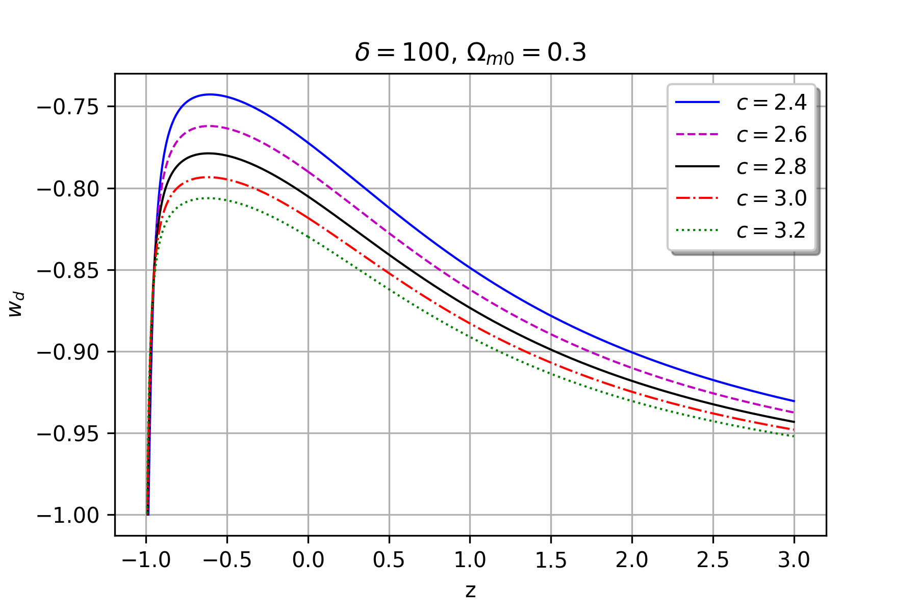
Figure 2: Behavior of $w_{d}$ vs $z$ for $H(z=0)=67.8,\quad M_{p}^{2}=1$ and varying  $c$ values.

Figures 1 and 2 show the EoS parameter behavior for the non interacting NTADE model. In plotting figure 1, the parameter $c$ is fixed at $3$ and $\delta$ is allowed to vary from 100 to 500. For figure 2, $c$ is allowed to vary by fixing $\delta$ at $100$. All the curves in the above two plots evolve in the quintessence region and finally, in the near or far future, meet the line $w_{d}=-1$. And hence, both the figures indicate that the non-interacting NTADE model is a pure quintessence model.

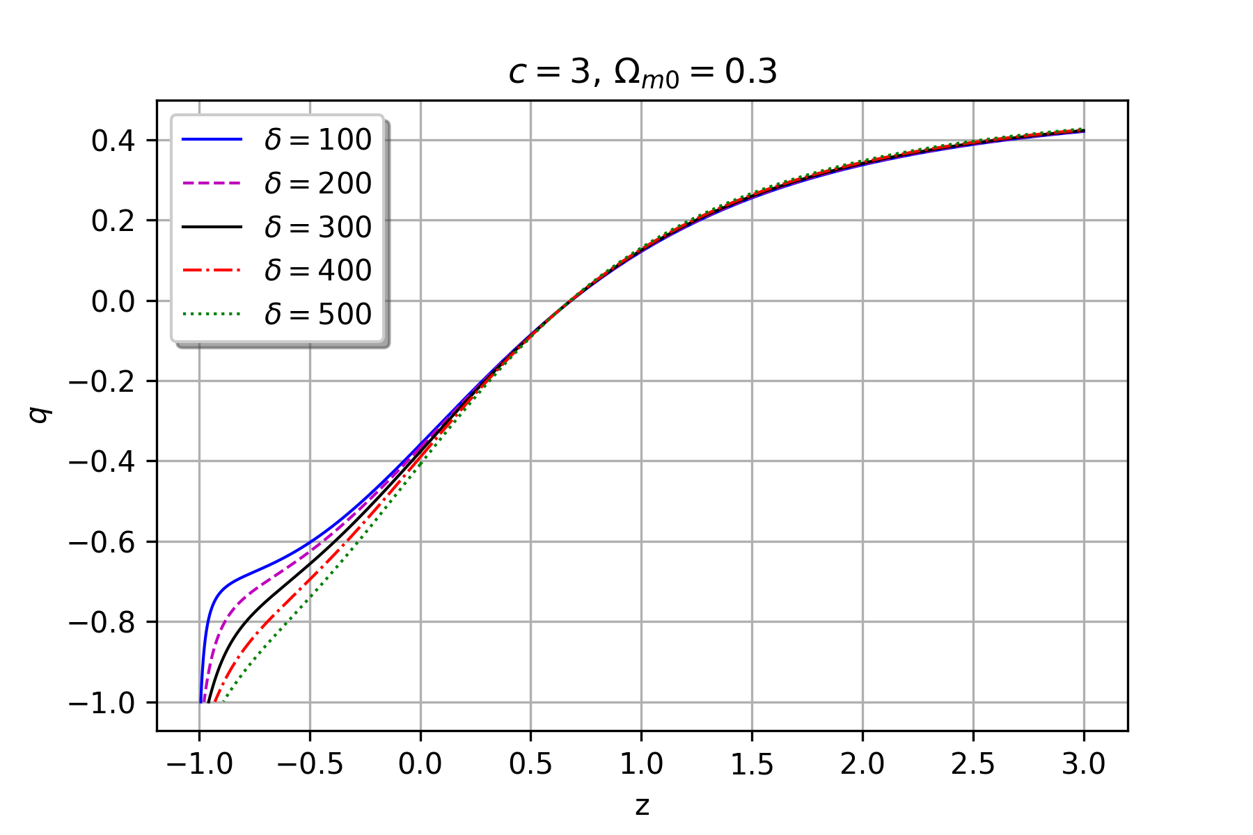
Figure 3: Behavior of $q$ vs $z$ for $H(z=0)=67.8,\quad M_{p}^{2}=1$ and varying values of $\delta$.

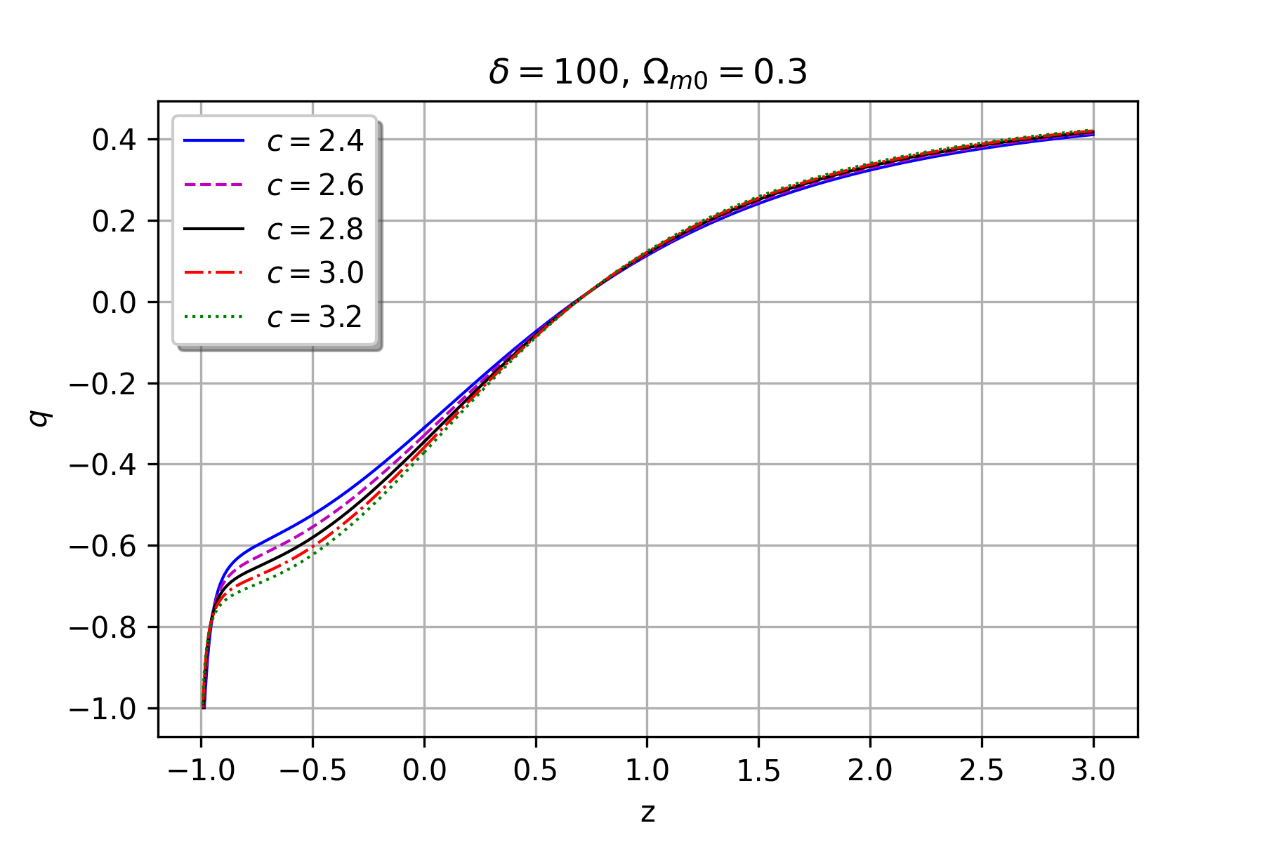
Figure 4: Behavior of $q$ vs $z$ for $H(z=0)=67.8, \quad M_{p}^{2}=1$ and prescribed $c$ values.

The deceleration parameter $q$ is plotted in figures 3-4. In plotting figure 3, $\delta$ is varying with $c=3$ whereas in figure 4, $c$ is allowed to vary by keeping $\delta$ at $100$. Curves in figure 3 and 4 indicate that the universe evolved from a decelerated phase. As $z$ approaches $0.6$ from right, the deceleration comes to an end. The acceleration started after $z\approx 0.6$.Clearly, the current universe is under accelerated expansion.

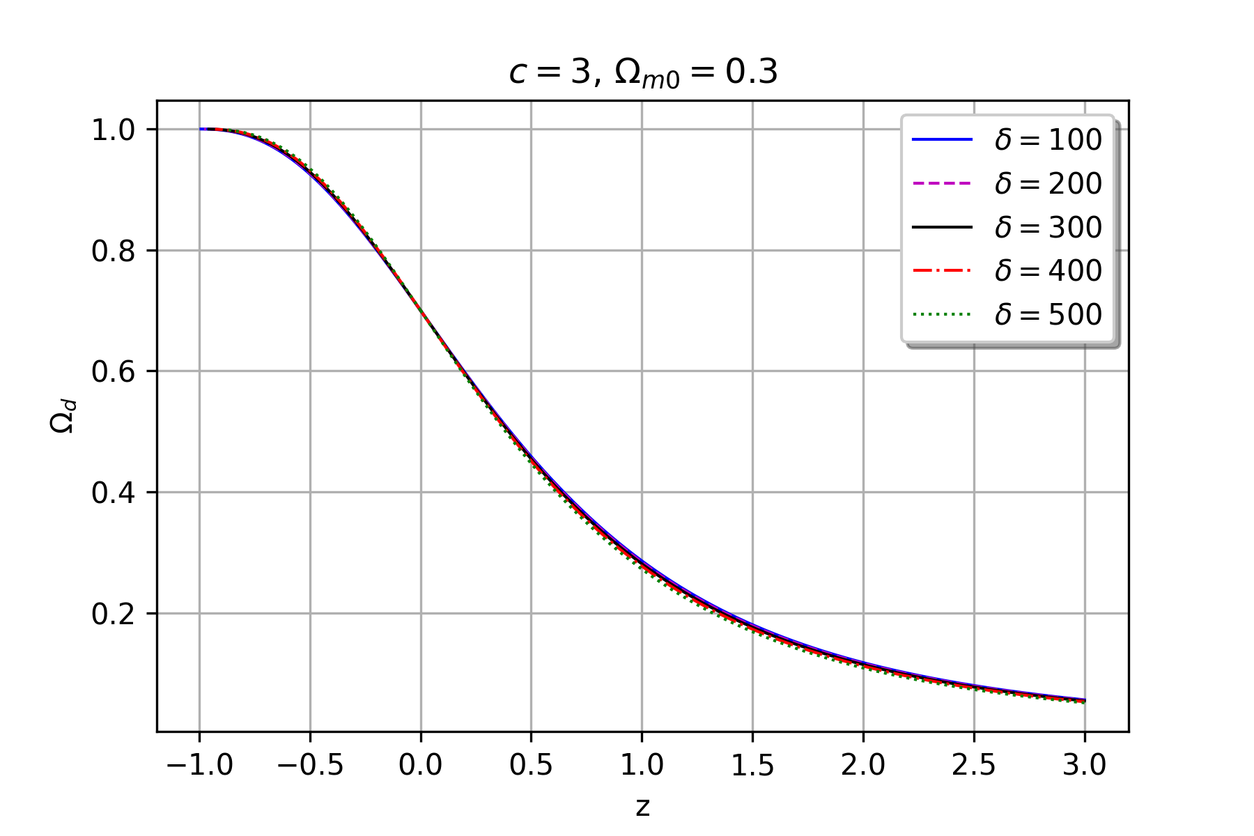
Figure 5: Behavior of $\Omega_{d}$ vs $z$ for $H(z=0)=67.8, \quad M_{p}^{2}=1$ and varying values of $\delta$.

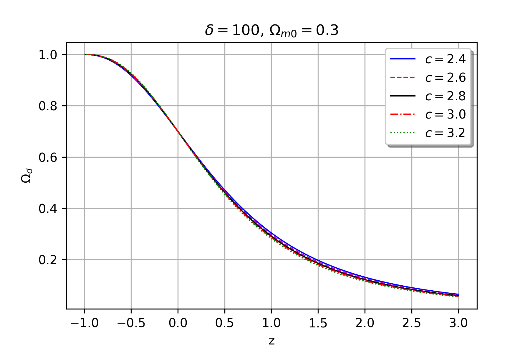
Figure 6: Behavior of $\Omega_{d}$ vs $z$ for $H(z=0)=67.8,\quad M_{p}^{2}=1$ and prescribed $c$ values.

Figures 5 and 6 are plotted for the NTADE density parameter $\Omega_{d}$ by considering variation in $\delta$ and in $c$, respectively.Both the curves show that the universe was dominated by DM in the past. Somewhere in $z\in(0.4,0.6)$, the NTADE started dominating and indicated to overtake fully in the near or far future.

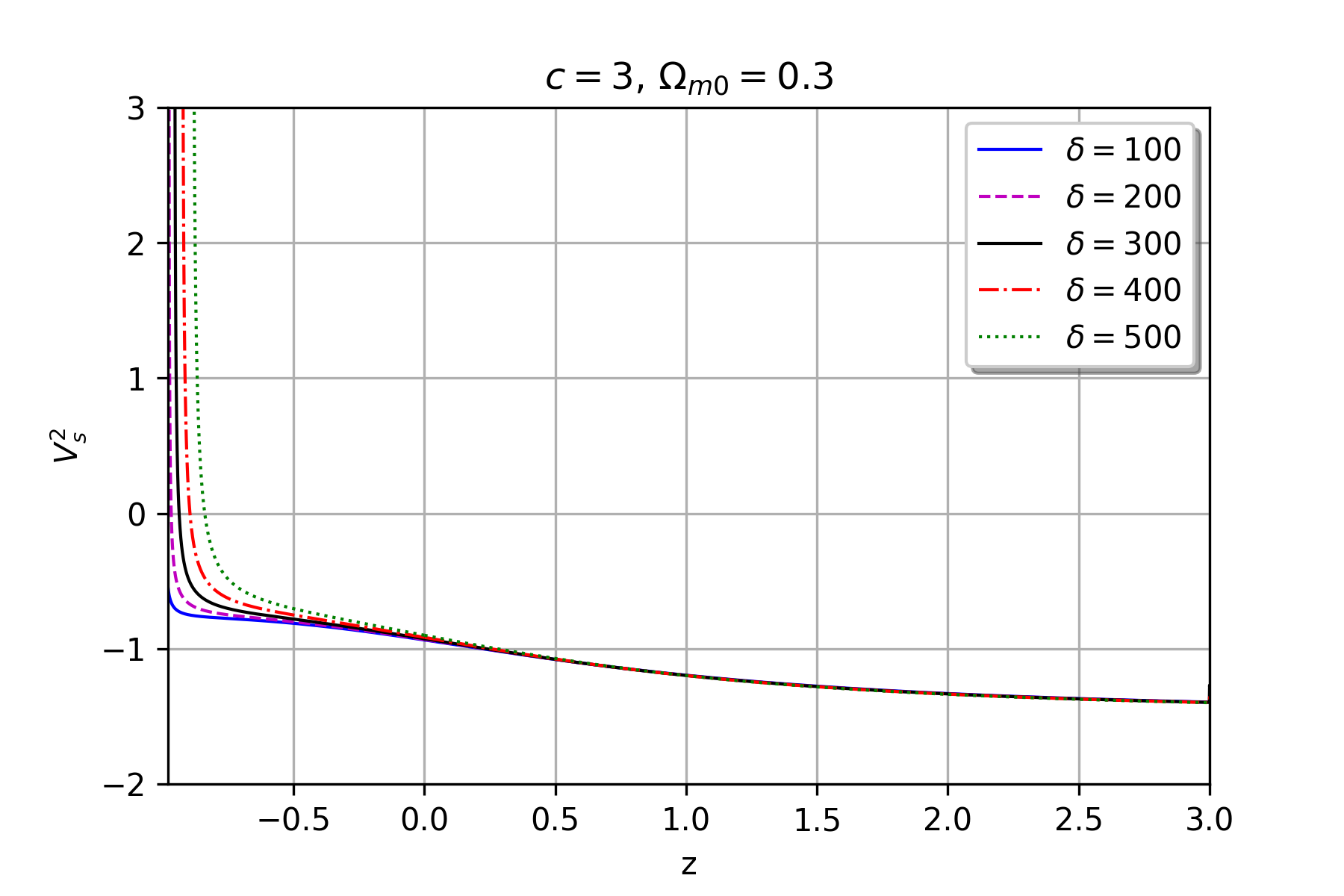
Figure 7: Behavior of $v_{s}^{2}$ vs $z$ for $H(z=0)=67.8,\quad M_{p}^{2}=1$ and prescribed values of $K$.

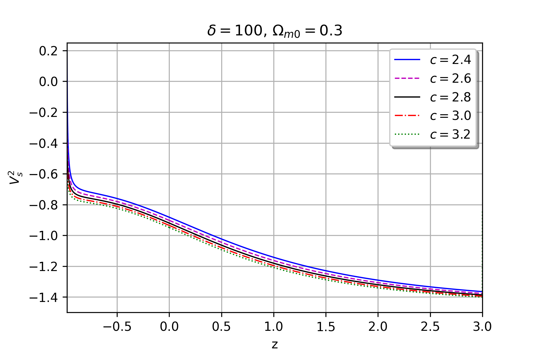
Figure 8: Behavior of $v_{s}^{2}$ vs $z$ for $H(z=0)=67.8,\quad M_{p}^{2}=1$ and prescribed values of $c$.

The squared sound speed plot in figures 7 and 8 show the non-interacting NTADE model to be unstable for current  cosmic behaviors.

4 Interacting NTADE Model

In this section the expressions are formulated by considering a flow of energy among the DM and DE sectors and hence the coupling term $Q$ appears with non-zero magnitude. Here we have chosen $Q=3b^{2}H(\rho_{d}+\rho_{m})$ [20, 39, 40, 53, 54, 55]. Differentiating (2) w.r.t. time and using equation (6), the expression for the EoS parameter is obtained as

$$w_{d} =-1-\dfrac{b^{2}}{\Omega_{d}}$$ (15)

$$-\dfrac{2}{3HT}\left(\dfrac{\delta^{2}M_{p}^{4}T^{4}-3c^{2}}{\delta^{2}M_{p}^{4}T^{4}+\delta M_{p}^{2}T^{2}+3c^{2}}\right),$$

where $T$ is given by (11).

Differentiating (7) w.r.t. time, using (6)and (8) we get

$$\frac{\dot{H}}{H^{2}} =\dfrac{3}{2}\left(-1+b^{2}+\Omega_{d}\right)$$ (16)

$$+\dfrac{\Omega_{d}}{HT}\left(\dfrac{\delta^{2}M_{p}^{4}T^{4}-3c^{2}}{\delta^{2}M_{p}^{4}T^{4}+\delta M_{p}^{2}T^{2}+3c^{2}}\right),$$

which leads to the deceleration parameter expression as

$$q=\dfrac{1}{2}\left(1-3b^{2}-3\Omega_{d}\right)$$

$$-\dfrac{\Omega_{d}}{HT}\left(\dfrac{\delta^{2}M_{p}^{4}T^{4}-3c^{2}}{\delta^{2}M_{p}^{4}T^{4}+\delta M_{p}^{2}T^{2}+3c^{2}}\right).$$ (17)

Taking time derivative of (9) and using (6), the differential equation for the NTADE density parameter is obtained as

$$\dot{\Omega_{d}}=2H(1+q)\Omega_{d}$$

$$+\dfrac{2\Omega_{d}}{T}\left(\dfrac{\delta^{2}M_{p}^{4}T^{4}-3c^{2}}{\delta^{2}M_{p}^{4}T^{4}+\delta M_{p}^{2}T^{2}+3c^{2}}\right).$$ (18)

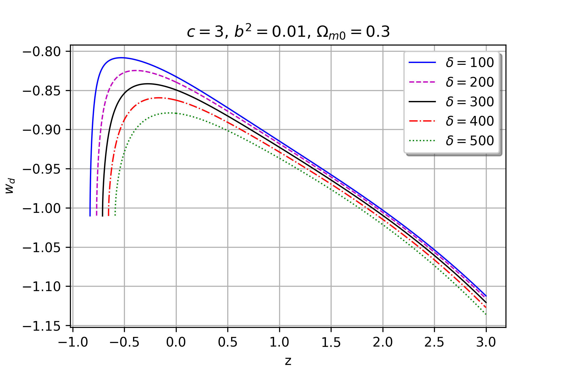
Figure 9: Behavior of $w_{d}$ vs $z$ for $H(z=0)=67.8,\quad M_{p}^{2}=1$ and prescribed values of $\delta$.

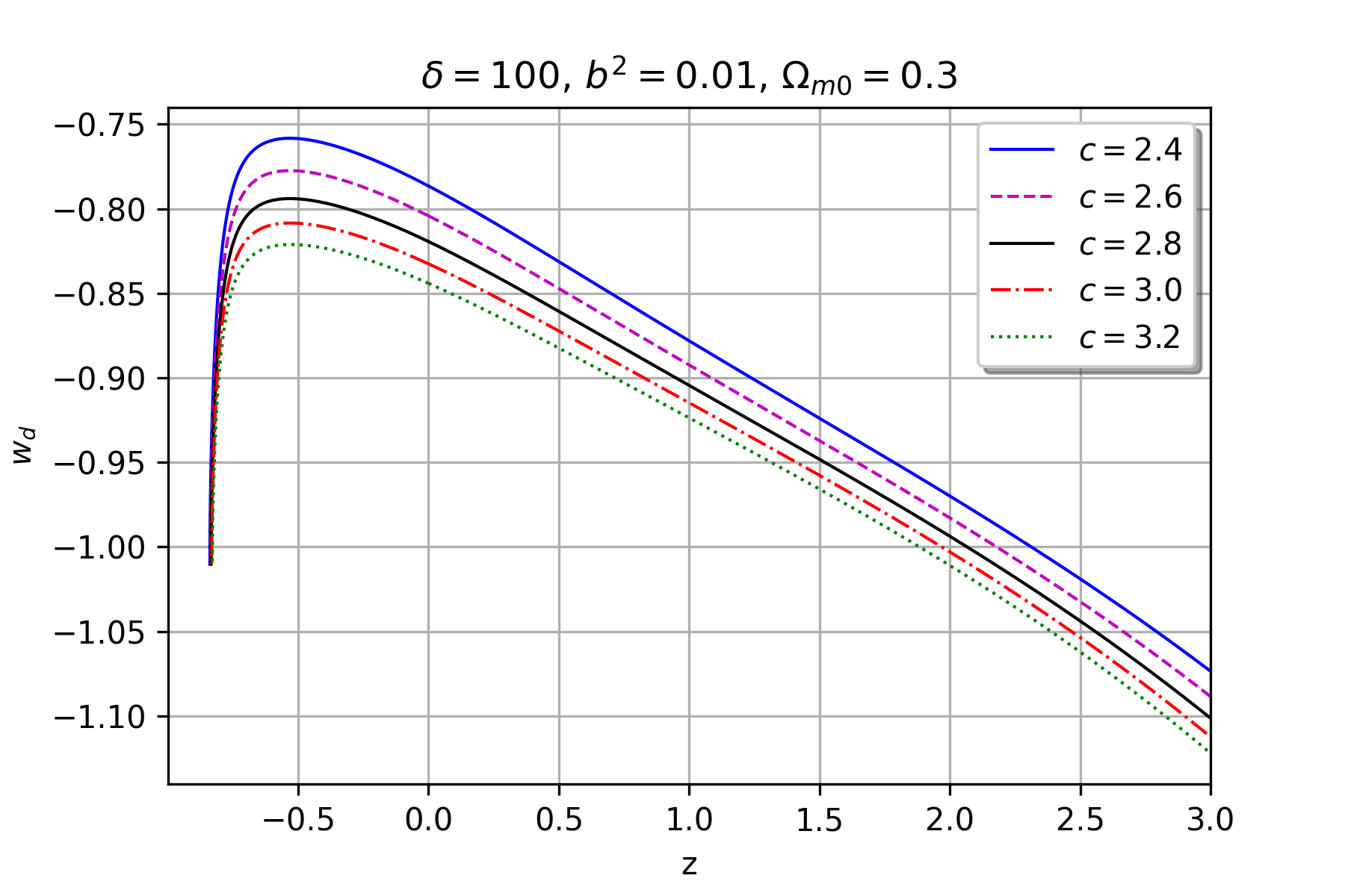
Figure 10: Behavior of $w_{d}$ vs $z$ for $H(z=0)=67.8,\quad M_{p}^{2}=1$ and prescribed values of $c$.

Figure 11: Behavior of $w_{d}$ vs $z$ for $H(z=0)=67.8,\quad M_{p}^{2}=1$ and prescribed values of $b^{2}$.

Behavior of the EoS parameter for interacting NTADE model is shown in figures 9-11. In figure 9, $\delta$ is varying with fixed $c$ and $b^{2}$. Similarly, figures 10 and 11 are plotted by varying $c$ and $b^{2}$, respectively by keeping the other two parameters fixed. Plots in figures 9-11 show that the universe evolved in a phantom region.  The present Universe rests in the quintessence zone and intends to cross the divide line $w_{d}=-1$ in near or far future to enter the phantom zone. In figure 11, the variation among the curves is more clear than others where $b^{2}$ is kept constant. This reflects appreciable features of the NTADE model on considering the interaction among the cosmos sectors.

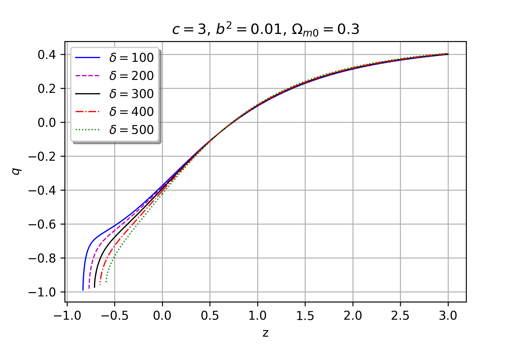
Figure 12: Behavior of $q$ vs $z$ for $H(z=0)=67.8,\quad M_{p}^{2}=1$ and prescribed values of $\delta$.

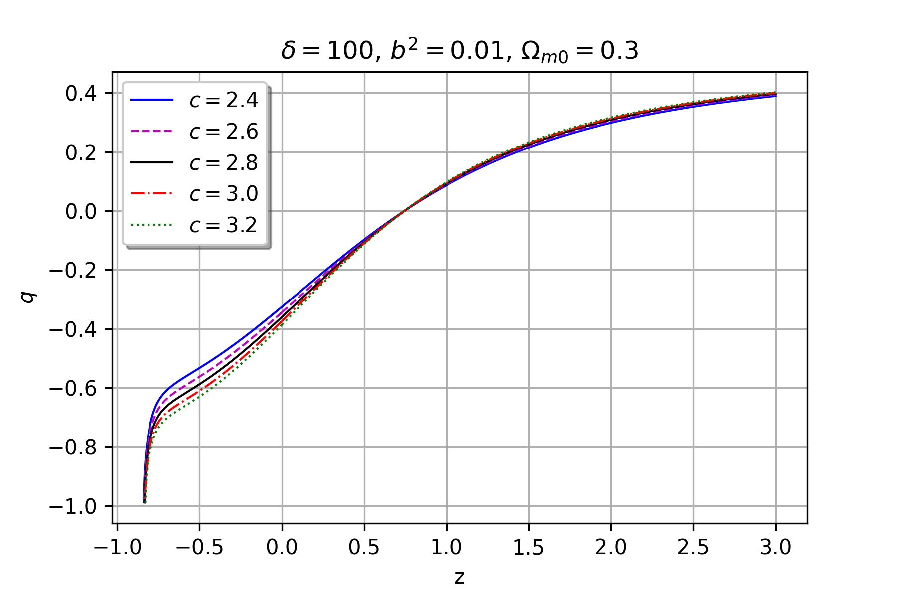
Figure 13: Behavior of $q$ vs $z$ for $H(z=0)=67.8,\quad M_{p}^{2}=1$ and prescribed values of $c$.

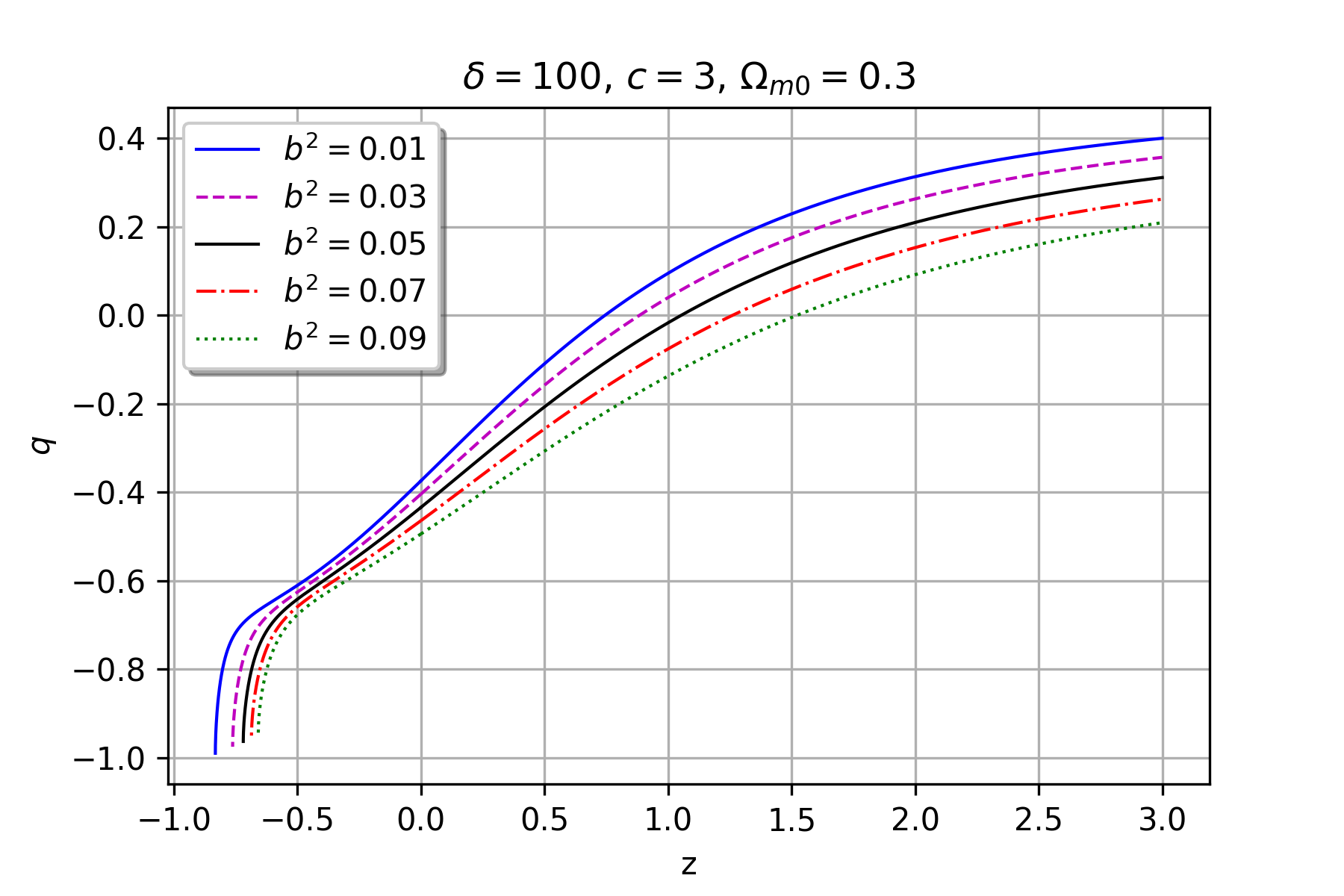
Figure 14: Behavior of $q$ vs $z$ for $H(z=0)=67.8,\quad M_{p}^{2}=1$ and prescribed values of $b^{2}$.

Figures 12-14 are showing the deceleration parameter behavior against the redshift $z$. Plots in 12 and 13 show that in the past, the universe faced the decelerated phase. And, somewhere in $z\in(0.5,0.8)$, it started accelerating. Both the figures confirm the current stage of the universe to be in accelerated expansion mode. Figure 14 is plotted by varying $b^{2}$, for fixed $c$ and $\delta$ values. 14 also supports the other two figures in telling the past of the universe to be in the decelerated phase. But, due to the presence of $b^{2}$ the curves show more variation and hence, the bound for $z\in(0.5,0.8)$ to enter the universe under accelerated expansion is no longer true, i.e. it widens the transit $z-$ range. But all three figures favor the current and future universe to be in an accelerated phase. As evident, the current $q$ value lies in $z\in(0.2,0.6)$.

Figure 15: Behavior of $\Omega_{d}$ vs $z$ for $H(z=0)=67.8,\quad M_{p}^{2}=1$ and prescribed values of $\delta$.

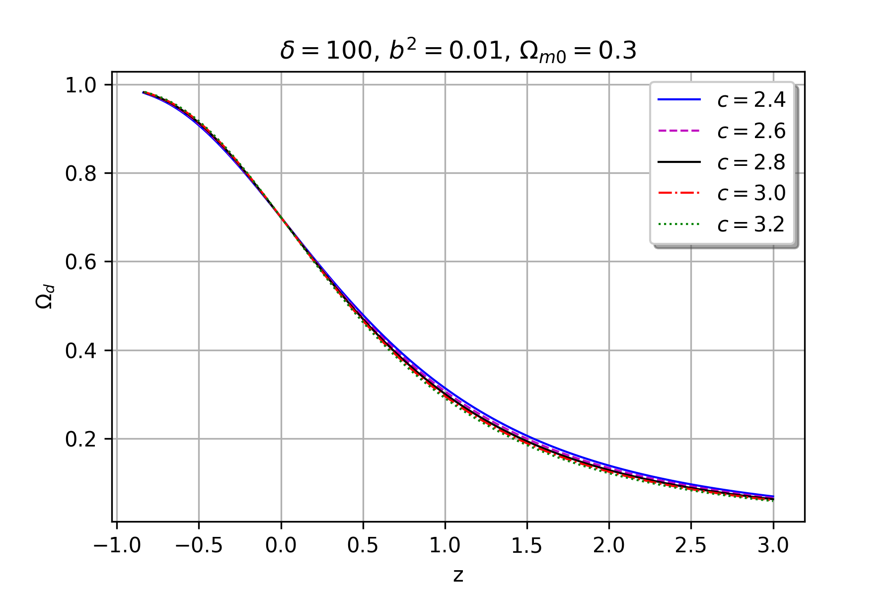
Figure 16: Behavior of $\Omega_{d}$ vs $z$ for $H(z=0)=67.8,\quad M_{p}^{2}=1$ and prescribed values of $c$.

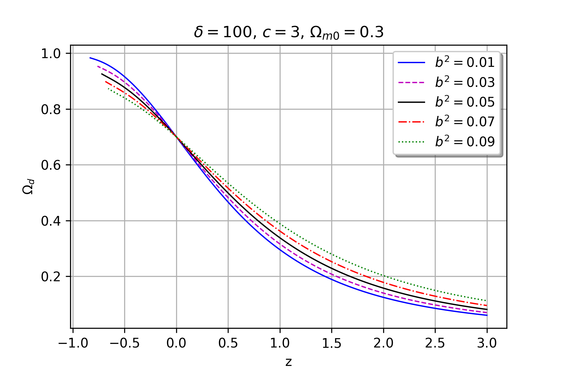
Figure 17: Behavior of $\Omega_{d}$ vs $z$ for $H(z=0)=67.8,\quad M_{p}^{2}=1$ and prescribed values of $b^{2}$.

The NTADE density parameter $\Omega_{d}$ explaining the evolutionary behavior of the universe is plotted in figures 15-17. It is clear that the universe in the past was fully dominated by the DM sector. But, by passage of time, NTADE started sharing with gradual increment somewhere in $z\gtrsim 0.5$  [56]. But the figure with $b^{2}$ variation shows the NTADE started overtaking the DM share in evolution of the universe somewhere in $z\in(0.2,0.5)$. All the curves in figures 15-17 reflect the current universe to be dominated by its NTADE constituent. They also indicate to occupy the whole share in near or far future by fully occupying the DM sector share.

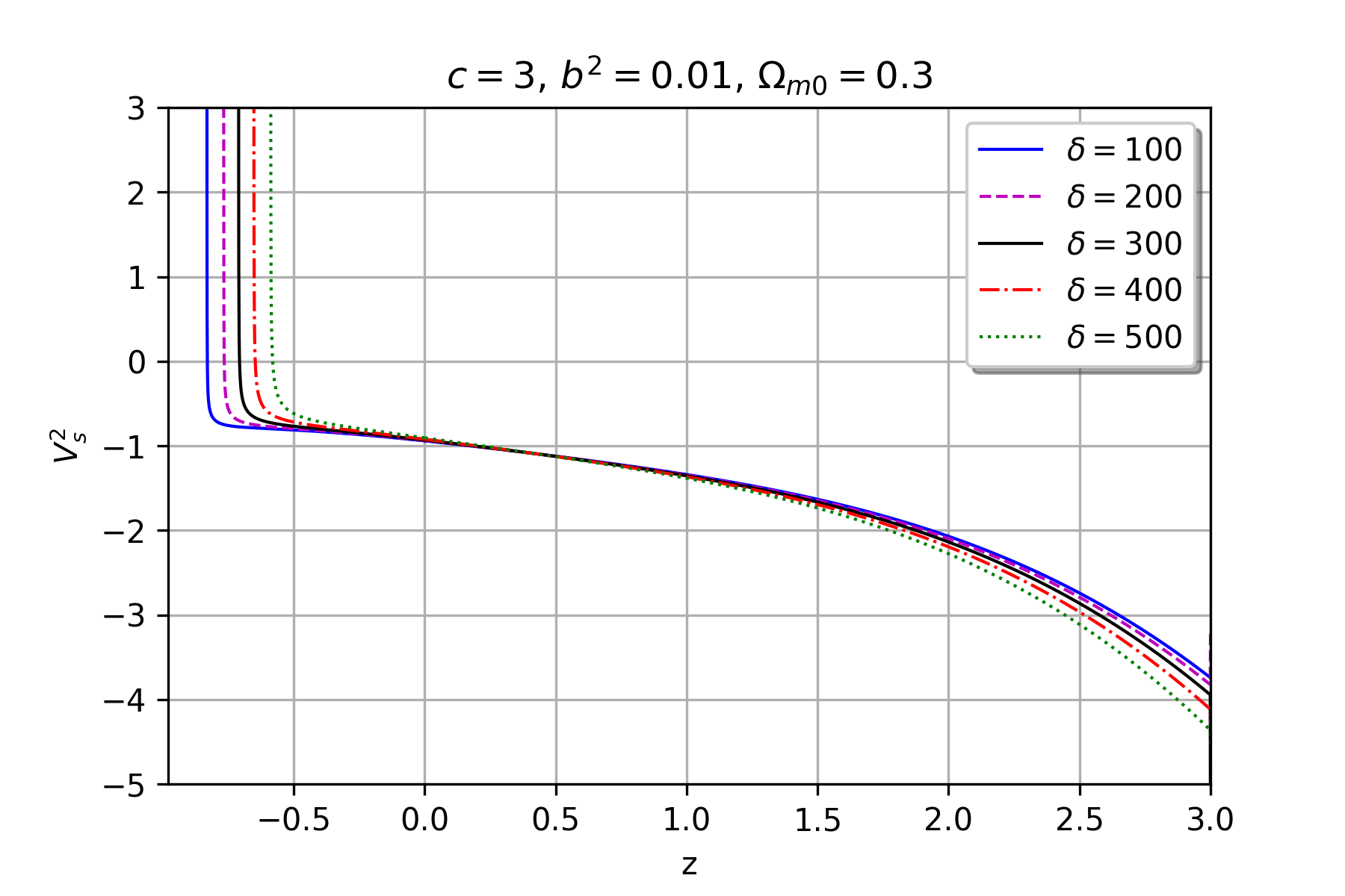
Figure 18: Behavior of $v_{s}^{2}$ vs $z$ for $H(z=0)=67.8,\quad M_{p}^{2}=1$ and prescribed values of $\delta$.

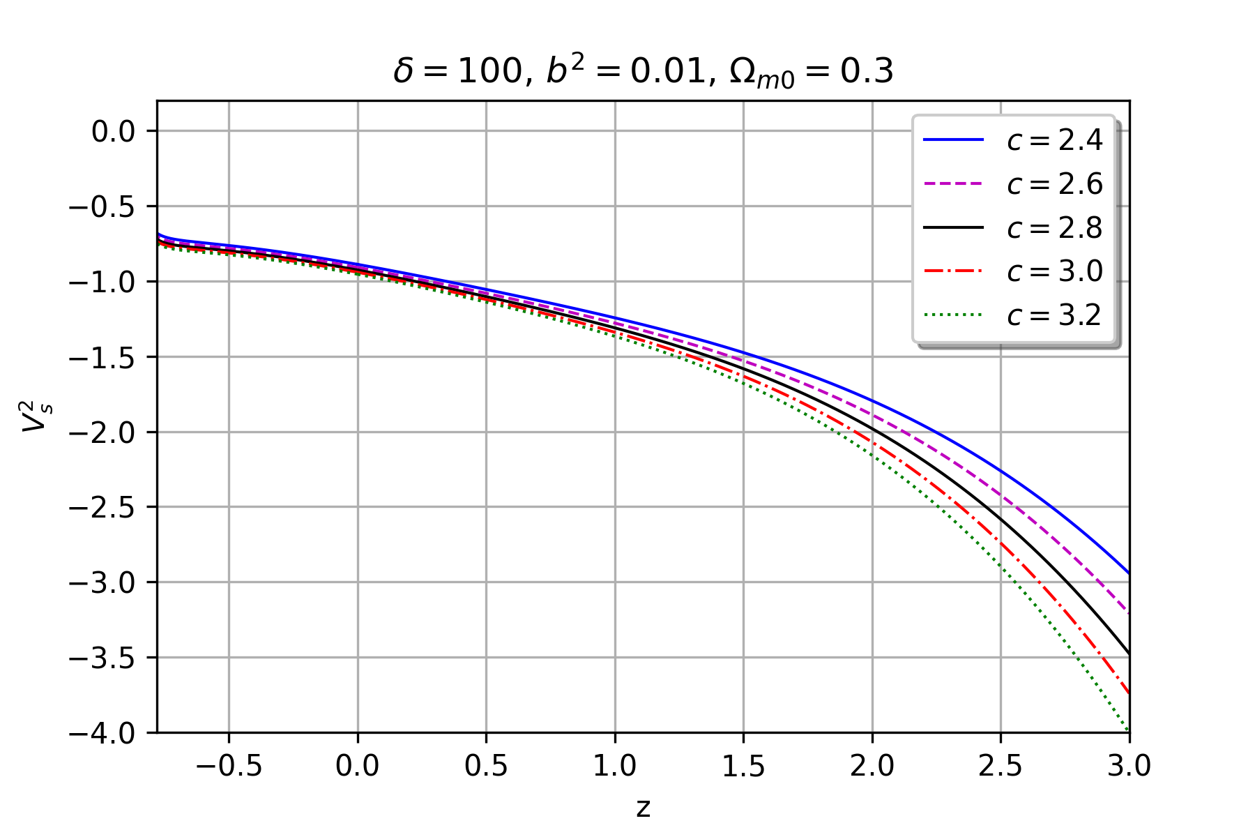
Figure 19: Behavior of $v_{s}^{2}$ vs $z$ for $H(z=0)=67.8,\quad M_{p}^{2}=1$ and prescribed values of $c$.

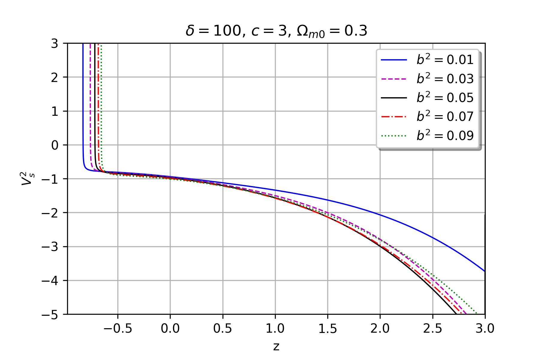
Figure 20: Behavior of $v_{s}^{2}$ vs $z$ for $H(z=0)=67.8,\quad M_{p}^{2}=1$ and prescribed values of $b^{2}$.

The squared sound speed is plotted in figures 18-20. These figures are plotted based on $\delta$, $c$ and $b^{2}$ variation respectively. These figures show that the NTADE model is efficient for future predictions of the universe.

5 Summary of the Results

To analyze the evolutionary behavior of the universe, we proposed the NTADE model as an alternative option to the holographic dark energy models. Being related to long-range interaction behavior of gravity, the non-extensive Tsallis entropy is used. Age of the universe is considered as IR cutoff instead of horizons. The  Karolyhazy uncertainty relation and the original ADE model [13] are the building blocks of the model. The model is studied by considering the independence among  DM and DE sectors constituting the universe as well as an interaction among them. The interaction term $Q$ linking the two sector features are also highlighted. In the case of $Q=0$, the NTADE model behaves like a pure quintessence model as evidenced from figures 1 and 2. But as the link between the two universe constituents is considered ($Q=3b^{2}H(\rho_{d}+\rho_{m})$), the behavior of the model becomes completely different. As depicted in figures 9-11 the interacting NTADE model behaves like Phantom in the past, quintessence at present and, again, becomes phantom by crossing the divide line $w_{d}=-1$ in near or far future. The deceleration parameter as depicted in figures 3 and 4 for non interacting cases shows the universe to enter accelerated phase for $z\approx 0.6$. But when interaction is considered, figures 12 and 13 indicate the accelerated expanding phase of the universe to happen somewhere in $z\in(0.2,1)$. The $b^{2}$ varying figure 14 shows a broad spectrum for $z$ and hence the interval $z\in(0.2,1)$ is no longer valid. Which shows further possibilities for the $z-$ range to be considered for the universe to transit into an accelerated phase. The current $q$ value found to be in $(-0.2,-0.5)$ for interacting as well as non interacting scenarios with constant $Q$. As $Q$ starts varying in figure 14, the current $q$ value shows more variation than the one considered in figures 3-4 and 12-13. The NTADE density parameter in figures 5-6 and 15-16 shows that the past of the universe was dominated by the matter sector $(z\gtrsim 0.5)$. But as $z$ became smaller the NTADE started overtaking the matter sector and reached to $\approx 70\%$ at present and shows the future of the universe to be fully dominated by the energy sector. For $b^{2}$ variation in figure 17, scenarios similar to other NTADE density figures are reflected. But, in this case, DM to NTADE takeover in $(z\gtrsim 0.5)$ is no longer valid. Although the Squared sound speed in figures 7-8  shows the instability of the non-interacting NTADE model, as the interaction comes to the picture, the model becomes stable for future $z$ values. And hence we can say, the interaction, i.e. the entry of the parameter $b^{2}$ increases the efficacy of the model.  The real range of parameters $\delta$, $c$ and $b^{2}$ are the open problems to be established by observational constraints.

References

- [1] A. G. Riess et al. [Supernova Search Team], “Observational evidence from supernovae for an accelerating universe and a cosmological constant,” Astron. J. 116, 1009-1038 (1998), [arXiv:astro-ph/9805201 [astro-ph]].
- [2] S. Perlmutter et al. [Supernova Cosmology Project], “Measurements of and from 42 high redshift supernovae,” Astrophys. J. 517, 565-586 (1999), [arXiv:astro-ph/9812133 [astro-ph]].
- [3] N. Aghanim et al. [Planck], “Planck 2018 results. VI. Cosmological parameters,” Astron. Astrophys. 641, A6 (2020) [erratum: Astron. Astrophys. 652, C4 (2021)], [arXiv:1807.06209 [astro-ph.CO]].
- [4] P. J. E. Peebles and B. Ratra, “The Cosmological Constant and Dark Energy,” Rev. Mod. Phys. 75, 559-606 (2003), [arXiv:astro-ph/0207347 [astro-ph]].
- [5] K. Bamba, S. Capozziello, S. Nojiri and S. D. Odintsov, “Dark energy cosmology: the equivalent description via different theoretical models and cosmography tests,” Astrophys. Space Sci. 342, 155-228 (2012), [arXiv:1205.3421 [gr-qc]].
- [6] S. Vagnozzi, L. Visinelli, P. Brax, A. C. Davis and J. Sakstein, “Direct detection of dark energy: The XENON1T excess and future prospects,” Phys. Rev. D 104, no.6, 063023 (2021), [arXiv:2103.15834 [hep-ph]].
- [7] G. K. Goswami, A. Pradhan and A. Beesham, “A Dark Energy Quintessence Model of the Universe,” Mod. Phys. Lett. A 35, no.04, 2050002 (2019), [arXiv:1905.10801 [gr-qc]].
- [8] T. Padmanabhan, “Cosmological constant: The Weight of the vacuum,” Phys. Rept. 380, 235-320 (2003) doi:10.1016/S0370-1573(03)00120-0 [arXiv:hep-th/0212290 [hep-th]].
- [9] V. Sahni and A. A. Starobinsky, “The Case for a positive cosmological Lambda term,” Int. J. Mod. Phys. D 9, 373-444 (2000) doi:10.1142/S0218271800000542 [arXiv:astro-ph/9904398 [astro-ph]].
- [10] E. J. Copeland, M. Sami and S. Tsujikawa, “Dynamics of dark energy,” Int. J. Mod. Phys. D 15, 1753-1936 (2006), [arXiv:hep-th/0603057 [hep-th]].
- [11] F. Karolyhazy, Nuovo Cim. A 42 (1966), 390-402 doi:10.1007/BF02717926, ; F. Karolyhazy, A. Frenkel and B. Lukacs, In Physics as natural Philosophy (Eds. A. Shimony and H. Feschbach, MIT Press, Cambridge,MA, 1982); F. Karolyhazy, A. Frenkel and B. Lukacs, In Quantum Concepts in Space and Time( Eds. R. Penrose and C.J. Isham, Clarendon Press, Oxford, 1986)
- [12] M. Maziashvili, “Space-time in light of Karolyhazy uncertainty relation,” Int. J. Mod. Phys. D 16, 1531-1539 (2007) doi:10.1142/S0218271807010870 [arXiv:gr-qc/0612110 [gr-qc]].
- [13] R. G. Cai, “A Dark Energy Model Characterized by the Age of the Universe,” Phys. Lett. B 657, 228-231 (2007), [arXiv:0707.4049 [hep-th]].
- [14] H. Wei and R. G. Cai, “A New Model of Agegraphic Dark Energy,” Phys. Lett. B 660, 113-117 (2008) doi:10.1016/j.physletb.2007.12.030 [arXiv:0708.0884 [astro-ph]].
- [15] L. Amendola, “Coupled quintessence,” Phys. Rev. D 62, 043511 (2000) doi:10.1103/PhysRevD.62.043511 [arXiv:astro-ph/9908023 [astro-ph]];
- [16] W. Zimdahl and D. Pavon, “Interacting quintessence,” Phys. Lett. B 521, 133-138 (2001) doi:10.1016/S0370-2693(01)01174-1 [arXiv:astro-ph/0105479 [astro-ph]].
- [17] L. P. Chimento, A. S. Jakubi, D. Pavon and W. Zimdahl, “Interacting quintessence solution to the coincidence problem,” Phys. Rev. D 67, 083513 (2003) doi:10.1103/PhysRevD.67.083513 [arXiv:astro-ph/0303145 [astro-ph]].
- [18] S. del Campo, R. Herrera, G. Olivares and D. Pavon, Phys. Rev. D 74, 023501 (2006) doi:10.1103/PhysRevD.74.023501 [arXiv:astro-ph/0606520 [astro-ph]].
- [19] B. Wang, E. Abdalla, F. Atrio-Barandela and D. Pavon, “Dark Matter and Dark Energy Interactions: Theoretical Challenges, Cosmological Implications and Observational Signatures,” Rept. Prog. Phys. 79, no.9, 096901 (2016) doi:10.1088/0034-4885/79/9/096901 [arXiv:1603.08299 [astro-ph.CO]].
- [20] D. Pavon and W. Zimdahl, “Holographic dark energy and cosmic coincidence,” Phys. Lett. B 628, 206-210 (2005) doi:10.1016/j.physletb.2005.08.134 [arXiv:gr-qc/0505020 [gr-qc]].
- [21] E. Di Valentino, A. Melchiorri, O. Mena and S. Vagnozzi, “Interacting dark energy in the early 2020s: A promising solution to the and cosmic shear tensions,” Phys. Dark Univ. 30, 100666 (2020), [arXiv:1908.04281 [astro-ph.CO]].
- [22] A. Gómez-Valent, V. Pettorino and L. Amendola, “Update on coupled dark energy and the tension,” Phys. Rev. D 101, no.12, 123513 (2020), [arXiv:2004.00610 [astro-ph.CO]].
- [23] V. Salvatelli, N. Said, M. Bruni, A. Melchiorri and D. Wands, “Indications of a late-time interaction in the dark sector,” Phys. Rev. Lett. 113, no.18, 181301 (2014) doi:10.1103/PhysRevLett.113.181301 [arXiv:1406.7297 [astro-ph.CO]].
- [24] H. Wei and R. G. Cai, “Interacting Agegraphic Dark Energy,” Eur. Phys. J. C 59, 99-105 (2009) doi:10.1140/epjc/s10052-008-0799-8 [arXiv:0707.4052 [hep-th]].
- [25] H. Wei and R. G. Cai, “Cosmological Constraints on New Agegraphic Dark Energy,” Phys. Lett. B 663, 1-6 (2008) doi:10.1016/j.physletb.2008.03.048 [arXiv:0708.1894 [astro-ph]].
- [26] J. L. Cui, L. Zhang, J. F. Zhang and X. Zhang, “New agegraphic dark energy as a rolling tachyon,” Chin. Phys. B 19, 019802 (2010) doi:10.1088/1674-1056/19/1/019802 [arXiv:0902.0716 [astro-ph.CO]].
- [27] H. R. Fazlollahi, “Agegraphic dark energy cosmology and Quantum loop-correction,” Phys. Dark Univ. 35, 100962 (2022).
- [28] Y. W. Kim, H. W. Lee, Y. S. Myung and M. I. Park, “New agegraphic dark energy model with generalized uncertainty principle,” Mod. Phys. Lett. A 23, 3049-3055 (2008) doi:10.1142/S021773230802848X [arXiv:0803.0574 [gr-qc]].
- [29] A. Sheykhi, “Interacting agegraphic dark energy models in a non-flat universe,” Phys. Lett. B 680, 113-117 (2009), [arXiv:0907.5144 [hep-th]].
- [30] A. Sheykhi, “Agegraphic Chaplygin gas model of dark energy,” Int. J. Mod. Phys. D 18, 2023-2034 (2009), [arXiv:1002.1435 [hep-th]].
- [31] X. Zhang, J. Zhang and H. Liu, “Agegraphic dark energy as a quintessence,” Eur. Phys. J. C 54, 303-309 (2008), [arXiv:0801.2809 [astro-ph]].
- [32] H. Wei and R. G. Cai, “Statefinder Diagnostic and w - w’ Analysis for the Agegraphic Dark Energy Models without and with Interaction,” Phys. Lett. B 655, 1-6 (2007), [arXiv:0707.4526 [gr-qc]].
- [33] M. Jamil and E. N. Saridakis, “New agegraphic dark energy in Horava-Lifshitz cosmology,” JCAP 07, 028 (2010), [arXiv:1003.5637 [physics.gen-ph]].
- [34] M. R. Setare and M. Jamil, “Statefinder diagnostic and stability of modified gravity consistent with holographic and new agegraphic dark energy,” Gen. Rel. Grav. 43, 293-303 (2011), [arXiv:1008.4763 [gr-qc]].
- [35] Y. Li, J. Ma, J. Cui, Z. Wang and X. Zhang, “Interacting model of new agegraphic dark energy: observational constraints and age problem,” Sci. China Phys. Mech. Astron. 54, 1367-1377 (2011), [arXiv:1011.6122 [astro-ph.CO]].
- [36] J. W. Gibbs, “Elementary Principles in Statistical Mechanics,” (New York, 1902).
- [37] C. Tsallis, “Possible Generalization of Boltzmann-Gibbs Statistics,” J. Statist. Phys. 52, 479-487 (1988) doi:10.1007/BF01016429
- [38] C. Tsallis and L. J. L. Cirto, “Black hole thermodynamical entropy,” Eur. Phys. J. C 73, 2487 (2013) doi:10.1140/epjc/s10052-013-2487-6 [arXiv:1202.2154 [cond-mat.stat-mech]].
- [39] M. Abdollahi Zadeh, A. Sheykhi and H. Moradpour, “Tsallis Agegraphic Dark Energy Model,” Mod. Phys. Lett. A 34, no.11, 1950086 (2019) doi:10.1142/S021773231950086X [arXiv:1810.12104 [physics.gen-ph]]
- [40] U. K. Sharma, G. Varshney and V. C. Dubey, “Barrow agegraphic dark energy,” Int. J. Mod. Phys. D 30, no.03, 2150021 (2021) doi:10.1142/S0218271821500218 [arXiv:2012.14291 [gr-qc]].
- [41] S. Srivastava, U. K. Sharma and V. C. Dubey, “Exploring the new Tsallis agegraphic dark energy with interaction through statefinder,” Gen. Rel. Grav. 53, no.4, 47 (2021), [arXiv:2105.02683 [gr-qc]].
- [42] H. Huang, Q. Huang and R. Zhang, “Phase space analysis of Tsallis agegraphic dark energy,” Gen. Rel. Grav. 53, no.7, 63 (2021).
- [43] Z. Feizi Mangoudehi, “Interacting Tsallis agegraphic dark energy in DGP braneworld cosmology,” Astrophys. Space Sci. 367, no.3, 31 (2022), [arXiv:2203.00492 [gr-qc]].
- [44] M. Kumar and A. K. Mishra, “Barrow holographic dark energy in Bianchi-I universe with k-essence,” Int. J. Geom. Meth. Mod. Phys. 19, no.05, 2250071 (2022).
- [45] U. K. Sharma and S. Srivastava, “The cosmological behavior and the statefinder diagnosis for the New Tsallis agegraphic dark energy,” Mod. Phys. Lett. A 35, no.38, 2050318 (2020), [arXiv:2105.07883 [gr-qc]].
- [46] A. Sardar and U. Debnath, “Cosmological consequences of Rényi, Sharma–Mittal holographic and new agegraphic dark energy models in generalized Rastall gravity,” Mod. Phys. Lett. A 36, no.25, 2150180 (2021).
- [47] S. Srivastava, V. C. Dubey and U. K. Sharma, “Statefinder diagnosis for Tsallis agegraphic dark energy model with - pair,” Int. J. Mod. Phys. A 35, no.06, 2050027 (2020).
- [48] Y. D. Xu, “Tsallis agegraphic dark energy model with the sign-changeable interaction,” Commun. Theor. Phys. 72, no.1, 015402 (2020).
- [49] S. Maity and U. Debnath, “Tsallis, Rényi and Sharma-Mittal holographic and new agegraphic dark energy models in D-dimensional fractal universe,” Eur. Phys. J. Plus 134, no.10, 514 (2019).
- [50] A. Pradhan and A. Dixit, “Tsallis holographic dark energy model with observational constraints in the higher derivative theory of gravity,” New Astron. 89, 101636 (2021).
- [51] M. Li, “A Model of holographic dark energy,” Phys. Lett. B 603, 1 (2004), [arXiv:hep-th/0403127 [hep-th]].
- [52] B. D. Pandey, S. K. P, Pankaj and U. K. Sharma, “New Tsallis holographic dark energy,” Eur. Phys. J. C 82, no.3, 233 (2022), [arXiv:2110.13628 [physics.gen-ph]].
- [53] J. Sadeghi, M. Khurshudyan, A. Movsisyan and H. Farahani, “Interacting Ghost Dark Energy Models with Variable and ,” JCAP 12, 031 (2013), [arXiv:1308.3450 [gr-qc]].
- [54] M. Honarvaryan, A. Sheykhi and H. Moradpour, “Thermodynamical description of the ghost dark energy model,” Int. J. Mod. Phys. D 24, no.07, 1550048 (2015), [arXiv:1505.01104 [gr-qc]].
- [55] G. K. Goswami, A. Pradhan and A. Beesham, “Friedmann–Robertson–Walker accelerating Universe with interactive dark energy,” Pramana 93, no.6, 89 (2019), [arXiv:1906.00450 [gr-qc]].
- [56] J. Frieman, M. Turner and D. Huterer, “Dark Energy and the Accelerating Universe,” Ann. Rev. Astron. Astrophys. 46, 385-432 (2008), [arXiv:0803.0982 [astro-ph]].