Markov Abstractions for PAC Reinforcement Learning in
Non-Markov Decision Processes

Abstract

Our work aims at developing reinforcement learning algorithms that do not rely on the Markov assumption. We consider the class of Non-Markov Decision Processes where histories can be abstracted into a finite set of states while preserving the dynamics. We call it a Markov abstraction since it induces a Markov Decision Process over a set of states that encode the non-Markov dynamics. This phenomenon underlies the recently introduced Regular Decision Processes (as well as POMDPs where only a finite number of belief states is reachable). In all such kinds of decision process, an agent that uses a Markov abstraction can rely on the Markov property to achieve optimal behaviour. We show that Markov abstractions can be learned during reinforcement learning. Our approach combines automata learning and classic reinforcement learning. For these two tasks, standard algorithms can be employed. We show that our approach has PAC guarantees when the employed algorithms have PAC guarantees, and we also provide an experimental evaluation.

1 Introduction

In the classic setting of Reinforcement Learning (RL), the agent is provided with the current state of the environment Sutton and Barto (2018). States are a useful abstraction for agents, since predictions and decisions can be made according to the current state. This is RL under the Markov assumption, or Markov RL. Here we focus on the more realistic non-Markov RL setting Hutter (2009); Brafman and De Giacomo (2019); Icarte et al. (2019); Ronca and De Giacomo (2021) where the agent is not given the current state, but can observe what happens in response to its actions. The agent can still try to regain the useful abstraction of states. However, now the abstraction has to be learned, as a map from every history observed by the agent to some state invented by the agent Hutter (2009).

We propose RL agents that learn a specific kind of abstraction called Markov abstraction as part of the overall learning process. Our approach combines automata learning and Markov RL in a modular manner, with Markov abstractions acting as an interface between the two modules. A key aspect of our contribution is to show how the sequence of intermediate automata built during learning induce partial Markov abstractions that can be readily used to guide exploration or exploitation. Our approach is Probably Approximately Correct (PAC), cf. Kearns and Vazirani (1994), whenever the same holds for the employed automata and Markov RL algorithms.

The idea of solving non-Markov tasks by introducing a Markovian state space can already be found in Bacchus et al. (1996) and more recently in Brafman et al. (2018); Icarte et al. (2018). RL in this setting has been considered Icarte et al. (2018); De Giacomo et al. (2019); Gaon and Brafman (2020); Xu et al. (2020). This setting is simpler than ours since transitions are still assumed to be Markov. The setting where both transitions and rewards are non-Markov has been considered in Icarte et al. (2019); Brafman and De Giacomo (2019), with RL studied in Icarte et al. (2019); Abadi and Brafman (2020); Ronca and De Giacomo (2021). Such RL techniques are based on automata learning. The approach in Ronca and De Giacomo (2021) comes with PAC guarantees, as opposed to the others which do not. Our approach extends the techniques in Ronca and De Giacomo (2021) in order to use the learned automata not only to construct the final policy, but also to guide exploration.

Abstractions from histories to states have been studied in Hutter (2009); Maillard et al. (2011); Veness et al. (2011); Nguyen et al. (2013); Lattimore et al. (2013); Hutter (2016); Majeed and Hutter (2018). Hutter (2009) introduces the idea of abstractions from histories to states. Its algorithmic solution, as well as the one in Veness et al. (2011), is less general than ours since it assumes a bound on the length of the histories to consider. This corresponds to a subclass of automata. Maillard et al. (2011) provides a technique to select an abstraction from a given finite set of candidate abstractions; instead, we consider an infinite set of abstractions. Nguyen et al. (2013) considers a set of abstractions without committing to a specific way of representing them. As a consequence, they are not able to take advantage of specific properties of the chosen representation formalism, in the algorithm nor in the analysis. On the contrary, we choose automata, which allows us to take advantage of existing automata-learning techniques, and in particular of their properties such as the incremental construction. Lattimore et al. (2013) studies non-Markov RL in the case where the non-Markov decision process belongs to a compact class. Their results do not apply to our case because the class of decision processes admitting a Markov abstraction is not compact. Majeed and Hutter (2018) studies Q-learning with abstractions, but it assumes that abstractions are given. Hutter (2016) provides a result that we use in Section 3; however, none of their abstractions is required to preserve the dynamics, as we require for our Markov abstractions. Even in the case called ‘exact state aggregation’, their abstractions are only required to preserve rewards, and not to preserve observations. In this setting, it is unclear whether automata techniques apply.

Proofs and experimental details are given in the appendix.

2 Preliminaries

For $x$ and $z$ strings, $xz$ denotes their concatenation. For $\Sigma$ and $\Gamma$ alphabets, $\Sigma\Gamma$ denotes the set of all strings $\sigma\gamma$ with $\sigma\in\Sigma$ and $\gamma\in\Gamma$. For $f$ and $g$ functions, $fg$ denotes their composition. We write $f:X\leadsto Y$ to denote a function $f:X\times Y\to[0,1]$ that defines a probability distribution $f(\cdot|x)$ over $Y$ for every $x\in X$.

Non-Markov Decision Processes.

A Non-Markov Decision Process (NMDP), cf. Brafman and De Giacomo (2019), is a tuple $\mathcal{P}=\langle A,O,R,\zeta,\mathbf{T},\mathbf{R}\rangle$ with components defined as follows. $A$ is a finite set of actions, $O$ is a finite set of observations, $R\subseteq\mathbb{R}_{\geq 0}$ is a finite set of non-negative rewards, $\zeta$ is a special symbol that denotes episode termination. Let the elements of $\mathcal{H}=(AOR)^{*}$ be called histories, and let the elements of $\mathcal{E}=(AOR)^{*}A\zeta$ be called episodes. Then, $\mathbf{T}:\mathcal{H}\times A\leadsto(O\cup\{\zeta\})$ is the transition function, and $\mathbf{R}:\mathcal{H}\times A\times O\leadsto R$ is the reward function. The transition and reward functions can be combined into the dynamics function $\mathbf{D}:\mathcal{H}\times A\leadsto(OR\cup\{\zeta\})$, which describes the probability to observe next a certain pair of observation and reward, or termination, given a certain history and action. Namely, $\mathbf{D}(or|h,a)=\mathbf{T}(o|h,a)\cdot\mathbf{R}(r|h,a,o)$ and $\mathbf{D}(\zeta|h,a)=\mathbf{T}(\zeta|h,a)$. We often write an NDMP directly as $\langle A,O,R,\zeta,\mathbf{D}\rangle$. A policy is a function $\pi:\mathcal{H}\leadsto A$. The uniform policy ${\pi_{\mathrm{u}}}$ is the policy defined as ${\pi_{\mathrm{u}}}(a|h)=1/|A|$ for every $a$ and every $h$. The dynamics of $\mathcal{P}$ under a policy $\pi$ describe the probability of an episode remainder, given the history so far, when actions are chosen according to a policy $\pi$; it can be recursively computed as $\mathbf{D}_{\pi}(aore|h)=\pi(a|h)\cdot\mathbf{D}(or|h,a)\cdot\mathbf{D}_{\pi}(e|haor)$, with base case $\mathbf{D}_{\pi}(a\zeta|h)=\pi(a|h)\cdot\mathbf{D}(\zeta|h,a)$. Since we study episodic reinforcement learning, we require episodes to terminate with probability one, i.e., $\sum_{e\in\mathcal{E}}\mathbf{D}_{\pi}(e|\varepsilon)=1$ for every policy $\pi$. This requirement ensures that the following value functions take a finite value. The value of a policy $\pi$ given a history $h$, written $\mathbf{v}_{\pi}(h)$, is the expected sum of future rewards when actions are chosen according to $\pi$ given that the history so far is $h$; it can be recursively computed as $\mathbf{v}_{\pi}(h)=\sum_{aor}\pi(a|h)\cdot\mathbf{D}(o,r|h,a)\cdot(r+\mathbf{v}_{\pi}(haor))$. The optimal value given a history $h$ is $\mathbf{v}_{*}(h)=\max_{\pi}\mathbf{v}_{\pi}(h)$, which can be expressed without reference to any policy as $\mathbf{v}_{*}(h)=\max_{a}\left(\sum_{or}\mathbf{D}(o,r|h,a)\cdot(r+\mathbf{v}_{*}(haor))\right)$. The value of an action $a$ under a policy $\pi$ given a history $h$, written $\mathbf{q}_{\pi}(h,a)$, is the expected sum of future rewards when the next action is $a$ and the following actions are chosen according to $\pi$, given that the history so far is $h$; it is $\mathbf{q}_{\pi}(h,a)=\sum_{or}\mathbf{D}(o,r|h,a)\cdot(r+\mathbf{v}_{\pi}(haor))$. The optimal value of an action $a$ given a history $h$ is $\mathbf{q}_{*}(h,a)=\max_{\pi}\mathbf{q}_{\pi}(h,a)$, and it can be expressed as $\mathbf{q}_{*}(h,a)=\sum_{or}\mathbf{D}(o,r|h,a)\cdot(r+\mathbf{v}_{*}(haor))$. A policy $\pi$ is optimal if $\mathbf{v}_{\pi}(\varepsilon)=\mathbf{v}_{*}(\varepsilon)$. For $\epsilon>0$, a policy $\pi$ is $\epsilon$-optimal if $\mathbf{v}_{\pi}(\varepsilon)\geq\mathbf{v}_{*}(\varepsilon)-\epsilon$.

Markov Decision Processes.

A Markov Decision Process (MDP) Bellman (1957); Puterman (1994) is a decision process where the transition and reward functions (and hence the dynamics function) depend only on the last observation in the history, taken to be an arbitrary observation when the history is empty. Thus, an observation is a complete description of the state of affairs, and it is customarily called a state to emphasise this aspect. Hence, we talk about a set $S$ of states in place of a set $O$ of observations. All history-dependent functions—e.g., transition and reward functions, dynamics, value functions, policies—can be seen as taking a single state in place of a history.

Episodic RL.

Given a decision process $\mathcal{P}$ and a required accuracy $\epsilon>0$, Episodic Reinforcement Learning (RL) for $\mathcal{P}$ and $\epsilon$ is the problem of an agent that has to learn an $\epsilon$-optimal policy for $\mathcal{P}$ from the data it collects by interacting with the environment. The interaction consists in the agent iteratively performing an action and receiving an observation and a reward in response, until episode termination. Specifically, at step $i$, the agent performs an action $a_{i}$, receiving a pair of an observation $o_{i}$ and a reward $r_{i}$, or the termination symbol $\zeta$, according to the dynamics of the decision process $\mathcal{P}$. This process generates an episode of the form $a_{1}o_{1}r_{1}a_{2}o_{2}r_{2}\dots a_{n}\zeta$. The collection of such episodes is the data available to the agent for learning.

Complexity Functions.

Describing the behaviour of a learning algorithm requires a way to measure the complexity of the instance $\mathcal{I}$ to be learned, in terms of a set of numeric parameters that reasonably describe the complexity of the instance—e.g., number of states of an MDP. Thus, for every instance $\mathcal{I}$, we have a list $\vec{c}_{\mathcal{I}}$ of values for the parameters. We use the complexity description to state properties for the algorithm by means of complexity functions. A complexity function $f$ is an integer-valued non-negative function of the complexity parameters and possibly of other parameters. Two distinguished parameters are accuracy $\epsilon>0$, and probability of failure $\delta\in(0,1)$. The dependency of complexity functions on these parameters is of the form $1/\epsilon$ and $\ln(1/\delta)$. When writing complexity functions, we will hide the specific choice of complexity parameters by writing $\mathcal{I}$ instead of $\vec{c}_{\mathcal{I}}$, and we will write $\epsilon$ and $\delta$ for $1/\epsilon$ and $\ln(1/\delta)$. For instance, we will write $f(\mathcal{I},\epsilon,\delta)$ in place of $f(\vec{c}_{\mathcal{I}},1/\epsilon,\ln(1/\delta))$.

Automata.

A Probabilistic Deterministic Finite Automaton (PDFA), cf. Balle et al. (2014), is a tuple $\mathcal{A}=\langle Q,\Sigma,\Gamma,\tau,\lambda,q_{0}\rangle$ where: $Q$ is a finite set of states; $\Sigma$ is a finite alphabet; $\Gamma$ is a finite set of termination symbols not in $\Sigma$; $\tau:Q\times\Sigma\to Q$ is the (deterministic) transition function; $\lambda:Q\times(\Sigma\cup\Gamma)\to[0,1]$ is the probability function, which defines a probability distribution $\lambda(\cdot|q)$ over $\Sigma\cup\Gamma$ for every state $q\in Q$; $q_{0}\in Q$ is the initial state. The iterated transition function $\tau^{*}:Q\times\Sigma^{*}\to Q$ is recursively defined as $\tau^{*}(q,\sigma_{1}\dots\sigma_{n})=\tau^{*}(\tau(q,\sigma_{1}),\sigma_{2}\dots\sigma_{n})$ with base case $\tau^{*}(q,\varepsilon)=q$; furthermore, $\tau^{*}(w)$ denotes $\tau^{*}(q_{0},w)$. It is required that, for every state $q\in Q$, there exists a sequence $\sigma_{1},\dots,\sigma_{n}$ of symbols of $\Sigma$ such that $\lambda(\tau^{*}(q,\sigma_{1}\dots\sigma_{i-1}),\sigma_{i})>0$ for every $i\in[1,n]$, and $\lambda(\tau(q,\sigma_{1}\dots\sigma_{n}),\gamma)>0$ for $\gamma\in\Gamma$—to ensure that every string terminates with probability one. Given a string $x\in\Sigma^{*}$, the automaton represents the probability distribution $\mathcal{A}(\cdot|x)$ over $\Sigma^{*}\Gamma$ defined recursively as $\mathcal{A}(\sigma y|x)=\lambda(\tau(x),\sigma)\cdot\mathcal{A}(y|x\sigma)$ with base case $\mathcal{A}(\gamma|x)=\lambda(\tau(x),\gamma)$ for $\gamma\in\Gamma$.

3 Markov Abstractions

Operating directly on histories is not desirable. There are exponentially-many histories in the episode length, and typically each history is observed few times, which does not allow for computing accurate statistics. A solution to this problem is to abstract histories to a reasonably-sized set of states while preserving the dynamics. We fix an NMDP $\mathcal{P}=\langle A,O,R,\zeta,\mathbf{D}\rangle$.

Definition 1.

A Markov abstraction over a finite set of states $S$ is a function $\alpha:\mathcal{H}\to S$ such that, for every two histories $h_{1}$ and $h_{2}$, $\alpha(h_{1})=\alpha(h_{2})$ implies $\mathbf{D}(\cdot|h_{1},a)=\mathbf{D}(\cdot|h_{2},a)$ for every action $a$.

Given an abstraction $\alpha$, its repeated application $\alpha^{*}$ transforms a given history by replacing observations by the corresponding states as follows:

$$\alpha^{*}(a_{1}o_{1}r_{1}\dots a_{n}o_{n}r_{n})=s_{0}a_{1}s_{1}r_{1}\dots a_{n}s_{n}r_{n},$$

$$\text{where }\,s_{i}=\alpha(h_{i})\text{ and }h_{i}=a_{1}o_{1}r_{1}\dots a_{i}o_{i}r_{i}.$$

Now consider the probability $P_{\alpha}(s_{i},r_{i}|h_{i-1},a_{i})$ obtained by marginalisation as:

$$P_{\alpha}(s_{i},r_{i}|h_{i-1},a_{i})=\sum_{o:\alpha(h_{i-1}a_{i}o)=s_{i}}\mathbf{D}(o,r_{i}|h_{i-1},a_{i}).$$

Since the dynamics $\mathbf{D}(o,r_{i}|h_{i-1},a_{i})$ are the same for every history mapped to the same state, there is an MDP $\mathcal{M}_{\mathcal{P}}^{\alpha}$ with dynamics $\mathbf{D}^{\alpha}$ such that $P_{\alpha}(s_{i}r_{i}|h_{i-1},a_{i})=\mathbf{D}^{\alpha}(s_{i}r_{i}|\alpha(h_{i-1}),a_{i})$. The induced MDP $\mathcal{M}_{\mathcal{P}}^{\alpha}$ can be solved in place of $\mathcal{P}$. Indeed, the value of an action in a state is the value of the action in any of the histories mapped to that state [Hutter, 2016, Theorem 1]. In particular, if $\pi$ is an $\epsilon$-optimal policy for $\mathcal{M}_{\mathcal{P}}^{\alpha}$, then $\pi\alpha$ is an $\epsilon$-optimal policy for $\mathcal{P}$.

3.1 Related Classes of Decision Processes

We discuss how Markov abstractions relate to existing classes of decision processes.

MDPs.

MDPs can be characterised as the class of NMDPs where histories can be abstracted into their last observation. Namely, they admit $\alpha(haor)=o$ as a Markov abstraction.

RDPs.

A Regular Decision Process (RDP) can be defined in terms of the temporal logic on finite traces $\textsc{ldl}_{f}$ Brafman and De Giacomo (2019) or in terms of finite transducers Ronca and De Giacomo (2021). The former case reduces to the latter by the well-known correspondence between $\textsc{ldl}_{f}$ and finite automata. In terms of finite transducers, an RDP is an NMDP $\mathcal{P}=\langle A,O,R,\zeta,\mathbf{D}\rangle$ whose dynamics function can be represented by a finite transducer $T$ that, on every history $h$, outputs the function $\mathbf{D}_{h}:A\leadsto(OR\cup\{\zeta\})$ induced by $\mathbf{D}$ when its first argument is $h$. Here we observe that the iterated version of the transition function of $T$ is a Markov abstraction.

POMDPs.

A Partially-Observable Markov Decision Process (POMDP), cf. Kaelbling et al. (1998), is a tuple $\mathcal{P}=\langle A,O,R,\zeta,X,\mathbf{T},\mathbf{R},\mathbf{O},x_{0}\rangle$ where: $A$, $O$, $R$, $\zeta$ are as in an NMDP; $X$ is a finite set of hidden states; $\mathbf{T}:X\times A\leadsto X$ is the transition function; $\mathbf{R}:X\times A\times O\leadsto R$ is the reward function; $\mathbf{O}:X\times A\times\leadsto(O\cup\{\zeta\})$ is the observation function; $x_{0}\in X$ is the initial hidden state. To define the dynamics function—i.e., the function that describes the probability to observe next a certain pair of observation and reward, or termination, given a certain history of observations and action—it requires to introduce the belief function $\mathbf{B}:\mathcal{H}\leadsto X$, which describes the probability of being in a certain hidden state given the current history. Then, the dynamics function can be expressed in terms of the belief function as $\mathbf{D}(or|h,a)=\sum_{x}\mathbf{B}(x|h)\cdot\mathbf{O}(o|x,a)\cdot\mathbf{R}(r|x,a,o)$ and $\mathbf{D}(\zeta|h,a)=\sum_{x}\mathbf{B}(x|h)\cdot\mathbf{O}(\zeta|x,a)$. Policies and value functions, and hence the notion of optimality, are as for NMDPs. For each history $h$, the probability distribution $\mathbf{B}(\cdot|h)$ over the hidden states is called a belief state. We note the following property of POMDPs.

Theorem 1.

If a POMDP has a finite set of reachable belief states, then the function that maps every history to its belief state is a Markov abstraction.

Proof sketch.

The function $\alpha(h)=\mathbf{B}(\cdot|h)$ is a Markov abstraction, as it can be verified by inspecting the expression of the dynamics function of a POMDP given above. Specifically, $\alpha(h_{1})=\alpha(h_{2})$ implies $\mathbf{B}(\cdot|h_{1})=\mathbf{B}(\cdot|h_{2})$, and hence $\mathbf{D}(\cdot|h_{1},a)=\mathbf{D}(\cdot|h_{2},a)$ for every action $a$. ∎

4 Our Approach to Non-Markov RL

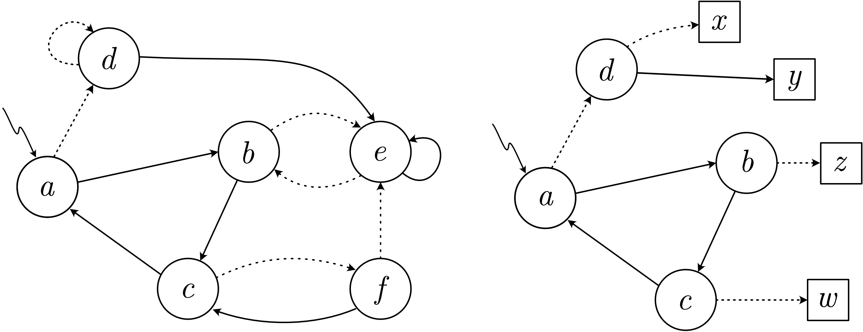
Figure 1: Target automaton (left), and hypothesis automaton (right). Solid edges denote transitions for input $1$, and dashed edges for $0$.

Our approach combines automata learning with Markov RL. We first describe the two modules separately, and then present the RL algorithm that combines them. For the section we fix an NMDP $\mathcal{P}=\langle A,O,R,\zeta,\mathbf{D}\rangle$, and assume that it admits a Markov abstraction $\alpha$ on states $S$.

4.1 First Module: Automata Learning

Markov abstractions can be learned via automata learning due to the following theorem.

Theorem 2.

There exist a transition function $\tau:S\times AOR\to S$ and an initial state $s_{0}$ such that, for every Markov policy $\pi$ on $S$, the dynamics $\mathbf{D}_{\pi\alpha}$ of $\mathcal{P}$ are represented by an automaton $\langle S,AOR,A\zeta,\tau,\lambda,s_{0}\rangle$ for some probability function $\lambda$. Furthermore, $\tau^{*}=\alpha$.

Proof sketch.

The start state is $s_{0}=\alpha(\varepsilon)$. The transition function is defined as $\tau(s,aor)=\alpha(h_{s}aor)$ where $h_{s}$ is an arbitrarily chosen history such that $\alpha(h_{s})=s$. Clearly $\tau^{*}=\alpha$. Then, the probability function is defined as $\lambda(s,aor)=\pi(a|s)\cdot\mathbf{D}(or|h_{s}a)$ and $\lambda(s,a\zeta)=\pi(a|s)\cdot\mathbf{D}(\zeta|h_{s}a)$. It can be shown by induction that the resulting automaton represents $\mathbf{D}_{\pi\alpha}$ regardless of the choice of the representative histories $h_{s}$, since all histories mapped to the same state determine the same dynamics function. ∎

We present an informal description of a generic PDFA-learning algorithm, capturing the essential features of the algorithms in Ron et al. (1998); Clark and Thollard (2004); Palmer and Goldberg (2007); Balle et al. (2013, 2014). We will highlight the characteristics that have an impact on the rest of the RL algorithm. To help the presentation, consider Figure 1. The figure shows the transition graph of a target automaton (left), and the hypothesis graph built so far by the algorithm (right). In the hypothesis graph we distinguish safe and candidate nodes. Safe nodes are circles in the figure. They are in a one-to-one correspondence with nodes in the target, they have all transitions defined, and they are not going to change. Candidate nodes are squares in the figure. Their transitions are not defined, and hence they form the frontier of the learned part of the graph. The graph is extended by promoting or merging a candidate. If the algorithm tests that a candidate node is distinct from every other safe state in the hypothesis graph, then it is promoted to safe. Upon promotion, a candidate is added for each possible transition from the just-promoted safe node. This effectively extends the automaton by pushing the frontier. If the algorithm tests that a candidate is equivalent to a safe node already in the hypothesis, then the candidate is merged into the safe node. The merge amounts to deleting the candidate node and redirecting all its incoming edges to the safe node. Thus, the statistical core of the algorithm consists in the tests. The test between two nodes is based on the input strings having prefixes that map to the two nodes respectively. A sufficient number of strings yields a good accuracy of the test. Assuming that all tests yield the correct result, it is easy to see that every new hypothesis is closer to the target. We focus on the approach in Balle et al. (2014), which has the following guarantees.

Guarantees 1.

There are complexity functions $K,N,T_{\mathrm{s}}$ such that, for every $\delta$ and every target automaton $\mathcal{A}$, the automata learning algorithm builds a sequence of hypotheses $\mathcal{A}_{1},\dots,\mathcal{A}_{n}$ satisfying the following conditions: (soundness) with probability at least $1-\delta$, for every $i\in[1,n]$, there is a transition-preserving bijection between the safe states of $\mathcal{A}_{i}$ and a subset of states of the target $\mathcal{A}$; (incrementality) for every $i\in[2,n]$, the hypothesis $\mathcal{A}_{i}$ contains all safe states and all transitions between safe states of $\mathcal{A}_{i-1}$; (liveness) every candidate $s$ is either promoted or merged within reading an expected number $K(\mathcal{A},\delta)$ of strings having a prefix that maps to $s$; (boundedness) the number $n$ of hypotheses is at most $N(\mathcal{A})$; (computational cost) every string $x$ is processed in time $T_{\mathrm{s}}(\mathcal{A},\delta,|x|)$.

We will ensure that statistics for a state $q$ are no longer updated once it is promoted to safe. This preserves the guarantees, and makes the algorithm insensitive to changes in the distribution $\lambda(q^{\prime},\cdot)$ of the target state $q^{\prime}$ corresponding to $q$ that take place after $q$ is promoted.

Since a hypothesis automaton $\mathcal{A}_{i}$ contains candidate states, that do not have outgoing transitions, the Markov abstraction $\alpha_{i}$ obtained as the iteration $\tau_{i}^{*}$ of its transition function is not a complete Markov abstraction, but a partial one. As a consequence, the MDP $\mathcal{M}_{i}$ induced by $\alpha_{i}$ is also partial. Specifically, it contains states from which one cannot proceed, the ones deriving from candidate nodes.

4.2 Second Module: Markov RL

When a Markov RL agent is confined to operate in a subset $S^{\prime}$ of the states $S$ of an MDP, it can always achieve one of two mutually-exclusive results. The first result is that it can find a policy that is near-optimal for the entire MDP, ignoring the states not in $S^{\prime}$. Otherwise, there is a policy that leads to a state not in $S^{\prime}$ sufficiently often. This is the essence of the Explore or Exploit lemma from Kearns and Singh (2002). The property is used explicitly in the $E^{3}$ algorithm Kearns and Singh (2002), and more implicitly in algorithms such as RMax Brafman and Tennenholtz (2002). Indeed, these algorithms can be employed to satisfy the following guarantees.

Guarantees 2.

There are complexity functions $E,T_{\mathrm{e}}$ such that, for every $\epsilon$, every $\delta$, and every MDP $\mathcal{M}$ where the agent is restricted to operate in a subset $S^{\prime}$ the states, the two following conditions hold: (explore or exploit) within $E(\mathcal{M},\epsilon,\delta)$ episodes, with probability at least $1-\delta$, either the agent finds an $\epsilon$-optimal policy or there is a state not in $S^{\prime}$ that is visited at least once; (computational cost) every episode $e$ is processed in time $T_{\mathrm{e}}(\mathcal{M},\epsilon,\delta,|e|)$.

4.3 Overall Approach

1 $\alpha\leftarrow\emptyset$;

2 loop  

3       $h\leftarrow\varepsilon$;

4       while $\alpha(h)$ is safe and episode is not over do

5             $a\leftarrow\mathtt{MarkovRL.choose}()$;

6             $o,r\leftarrow$ perform action $a$;

7             $\mathtt{MarkovRL.observe}(\alpha(h),a,r,\alpha(haor))$;

8             $h\leftarrow haor$;

9      while episode is not over do

10             $a\leftarrow$ pick an action according to $\pi_{\mathrm{u}}$;

11             $o,r\leftarrow$ perform action $a$;

12             $h\leftarrow haor$;

13      $\alpha\leftarrow\mathtt{AutomataLearning.consume}(h)$;

14       $\mathtt{MarkovRL.update}(\alpha)$;

15      

Algorithm 1 NonMarkovRL

We will have a Markov agent operating in the MDP induced by the current partial abstraction, in order to either find a near-optimal policy (when the abstraction is sufficiently complete) or to visit candidate states (to collect strings to extend the abstraction). Concretely, we propose Algorithm 1, that employs the modules $\mathtt{AutomataLearning}$ and $\mathtt{MarkovRL}$ to solve non-Markov RL. It starts with an empty abstraction $\alpha$ (Line 1), and then it loops, processing one episode per iteration. Line 3 corresponds to the beginning of an episode, and hence the algorithm sets the current history to the empty history. Lines 4–8 process the prefix of the episode that maps to the safe states; on this prefix, the Markov RL agent is employed. Specifically, the agent is first queried for the action to take (Line 5), the action is then executed (Line 6), the resulting transition is shown to the agent (Line 7), and the current history is extended (Line 8). Lines 9–12 process the remainder of the episode, for which we do not have an abstraction yet. First, an action is chosen according to the uniform policy $\pi_{\mathrm{u}}$ (Line 10), the action is then executed (Line 11), and the current history is extended (Line 12). Lines 13–14 process the episode that has just been generated, before moving to the next episode. In Line 13 the automata learning algorithm is given the episode, and it returns the possibly-updated abstraction $\alpha$. Finally, in Line 14, the Markov agent is given the latest abstraction, and it has to update its model and/or statistics to reflect any change in the abstraction. We assume a naive implementation of the update function, that amounts to resetting the Markov agent when the given abstraction is different from the previous one.

The algorithm has PAC guarantees assuming PAC guarantees for the employed modules. In particular, let $K,N,T_{\mathrm{s}}$ be as in Guarantees 1, and let $E,T_{\mathrm{e}}$ be as in Guarantees 2. In the context of Algorithm 1, the target automaton is the automaton $\mathcal{A}^{\mathrm{u}}_{\mathcal{P}}$ that represents the dynamics of $\mathcal{P}$ under the uniform policy ${\pi_{\mathrm{u}}}$, and the MDP the Markov agent interacts with is the MDP $\mathcal{M}^{\alpha}_{\mathcal{P}}$ induced by $\alpha$. Furthermore, let $L_{\mathcal{P}}$ be the expected episode length for $\mathcal{P}$.

Theorem 3.

For any given $\epsilon$ and $\delta$, and for any NMDP $\mathcal{P}$ admitting a Markov abstraction $\alpha$, Algorithm 1 has probability at least $1-\delta$ of solving the Episodic RL problem for $\mathcal{P}$ and $\epsilon$, using a number of episodes

$$O\big{(}N(\mathcal{A}^{\mathrm{u}}_{\mathcal{P}})\cdot\left\lceil E(\mathcal{M}_{\mathcal{P}}^{\alpha},\epsilon,\delta^{\prime})/K(\mathcal{A}^{\mathrm{u}}_{\mathcal{P}},\delta/2)\right\rceil\big{)}$$

with $\delta^{\prime}=\delta/(2\cdot N(\mathcal{A}^{\mathrm{u}}_{\mathcal{P}}))$, and a number of computation steps that is proportional to the number of episodes by a quantity

$$O\big{(}T_{\mathrm{s}}(\mathcal{A}^{\mathrm{u}}_{\mathcal{P}},\delta/2,L_{\mathcal{P}})+T_{\mathrm{e}}(\mathcal{M}_{\mathcal{P}}^{\alpha},\epsilon,\delta^{\prime},L_{\mathcal{P}})\big{)}.$$

Proof sketch.

An execution of the algorithm can be split into stages, with one stage for each hypothesis automaton. By the boundedness condition, there are at most $N(\mathcal{A}^{\mathrm{u}}_{\mathcal{P}})$ stages. Consider an arbitrary stage. Within $E(\mathcal{M}_{\mathcal{P}}^{\alpha},\epsilon,\delta^{\prime})$ episodes, the Markov agent either exploits or explores. If it exploits, i.e., it finds an $\epsilon$-optimal policy $\pi$ for the MDP induced by the current partial abstraction $\alpha_{i}$, then $\pi\alpha_{i}$ is $\epsilon$-optimal for $\mathcal{P}$. Otherwise, a candidate state is explored $K(\mathcal{A}^{\mathrm{u}}_{\mathcal{P}},\delta/2)$ times, and hence it is promoted or merged. The probability $\delta$ of failing is partitioned among the one run of the automata learning algorithm, and the $N(\mathcal{A}^{\mathrm{u}}_{\mathcal{P}})$ independent runs of the Markov RL algorithm. Regarding the computation time, note that the algorithm performs one iteration per episode, it operates on one episode in each iteration, calling the two modules and performing some other operations having a smaller cost. ∎

(a) Reset-Rotating MAB

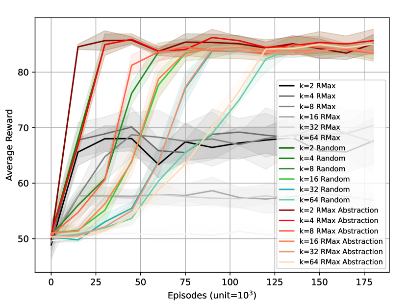
(b) Enemy Corridor

(c) Flickering Grid

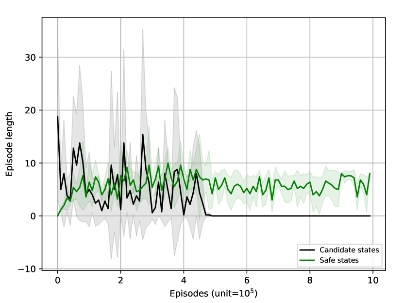
(d) Safe vs. candidate states

(e) Rotating MAB

(f) Malfunction MAB

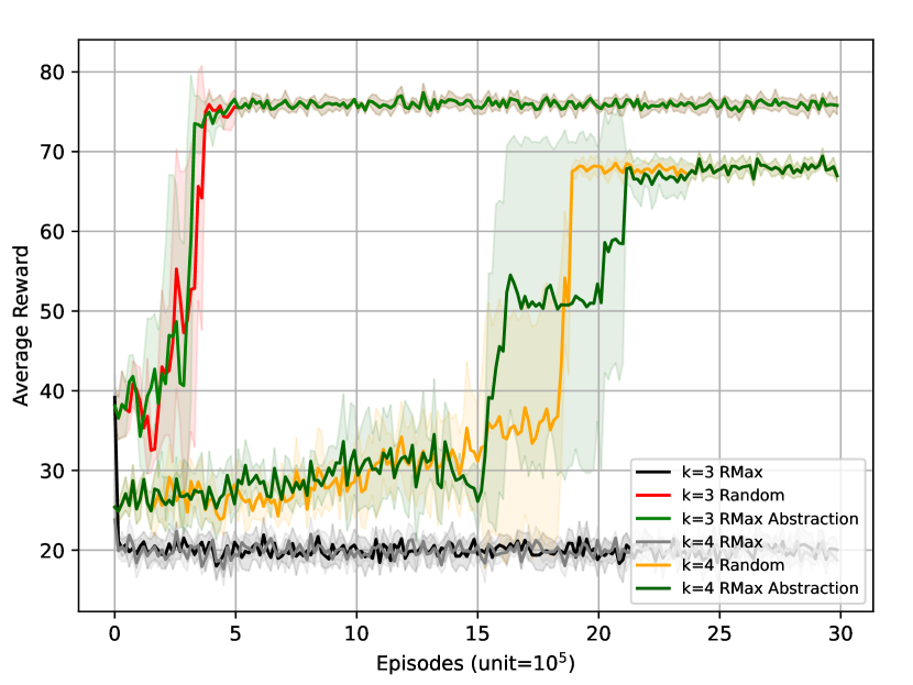
(g) Cheat MAB

(h) Rotating Maze

Figure 2: Empirical evaluation of Markov Abstractions.

5 Empirical Evaluation

We show an experimental evaluation of our approach. We employ the state-of-the-art stream PDFA learning algorithm Balle et al. (2014) and the classic RMax algorithm Brafman and Tennenholtz (2002). They satisfy Guarantees 1 and 2. We consider the domains from Abadi and Brafman (2020): Rotating MAB, Malfunction MAB, Cheat MAB, and Rotating Maze; a variant of Enemy Corridor Ronca and De Giacomo (2021); and two novel domains: Reset-Rotating MAB, and Flickering Grid. Reset-Rotating MAB is a variant of Rotating MAB where failing to pull the correct arm brings the agent back to the initial state. Flickering Grid is a basic grid with an initial and a goal position, but where at some random steps the agent is unable to observe its position. All domains are parametrised by $k$, which makes the domains more complex as it is assigned larger values.

Figure 2 shows our performance evaluation. Plots include three different approaches. First, our approach referred to as RMax Abstraction, i.e., the RMax Markov agent provided with partial Markov abstractions as they are incrementally learned. Second, a Random Sampling approach, equivalent to what is proposed in Ronca and De Giacomo (2021), that always explores at random. Third, the RMax agent as a baseline for the performance of a purely Markov agent, that does not rely on Markov abstractions. Results for each approach are averaged over 5 trainings and show the standard deviation. At each training, the agent is evaluated at every 15k training episodes. Each evaluation is an average over 50 episodes, where for each episode we measure the accumulated reward divided by the number of steps taken. Notice that the RMax Abstraction agent takes actions uniformly at random on histories where the Markov abstraction is not yet defined, otherwise taking actions greedily according to the value function.

The results for Reset-Rotating MAB (Figure 2(a)) show the advantage of the exploration strategy of our approach, compared to Random Sampling. In fact, in this domain, random exploration does not allow for exploring states that are far from the initial state. The results for Enemy Corridor (Figure 2(b)) show that our approach scales with the domain size. Namely, in Enemy Corridor we are able to increase the corridor size $k$ up to $64$. The results for Flickering Grid (Figure 2(c)) show that our approach works in a domain with partial observability, that is natural to model as a POMDP. This is in line with our Theorem 1. The Markov abstraction for Flickering Grid maps histories to the current cell; intuitively, the agent learns to compute its position even if sometimes it is not explicitly provided by the environment. For this domain, Figure 2(d) shows the number of steps the agent is in a safe state against when it is not. The figure exemplifies the incremental process of learning a Markov abstraction, as the time spent by the agent out of the safe region is high during the first episodes, and it decreases as more histories are collected and more safe states get to be learned by the stream PDFA learning algorithm; we see the agent achieves optimal behaviour around $5\cdot 10^{5}$ episodes, when it no longer encounters candidate states, since all relevant states have been learned.

In the domains from Abadi and Brafman (2020) (Figures 2(e)-2(h)) our approach has poor performance overall. We are able to show convergence in all domains except Rotating Maze with $k=2,3$ and Malfunction MAB with $k=5$. However, it requires a large number of episodes before achieving a close-to-optimal average reward. We observe that all these domains have a low distinguishability between the probability distribution of the states. The performance of PDFA-learning is greatly dependent on such parameter, cf. Balle et al. (2013). Furthermore, in these domains, the value of distinguishability decreases with $k$. On the contrary, in Reset-Rotating MAB, Enemy Corridor, and Flickering Grid, distinguishability is high and independent of $k$. Therefore, we conclude that a low distinguishability is the source of poor performance. In particular, it causes the automata learning module to require a large number of samples.

We compare our approach against two related approaches. First, we compare against Abadi and Brafman (2020) that combines deterministic finite automata learning with history clustering to build a Mealy Machine that represents the underlying decision process, while employing MCTS to compute policies for the learned models. Comparing to the results published in Abadi and Brafman (2020) for Rotating MAB, Malfuction MAB, and Rotating Maze, our approach has better performance in Rotating MAB, and worse performance in the other domains. Second, we compare against Icarte et al. (2019), also based on automata learning. Our approach outperforms theirs in all the domains mentioned in this paper, and their approach outperforms ours in all their domains. Specifically, their algorithm does not converge in our domains, and our algorithm does not converge in theirs. Our poor performance is explained by the fact that all domains in Icarte et al. (2019) have a low distinguishability, unfavourable to us. On the other hand, their poor performance in our domains might be due to their reliance on local search methods.

6 Conclusion and Future Work

We presented an approach for learning and solving non-Markov decision processes, that combines standard RL with automata learning in a modular manner. Our theoretical results show that, for NMDPs that admit a Markov abstraction, $\epsilon$-optimal policies can be computed with PAC guarantees, and that its dynamics can be accurately represented by an automaton. The experimental evaluation shows the feasibility of the approach. The comparison with the random-exploration baseline shows the advantage of a smarter exploration based on the automaton as it is still being learned, which is an important aspect introduced in this paper. Some of the domains illustrate the difficulty of learning when distinguishability is low—an issue of the underlying automata learning algorithm. At the same time, other domains show good scalability of the overall approach when distinguishability stays high.

The difficulties encountered by the PDFA-learning algorithm in domains with low distinguishability suggest that the existing PDFA-learning techniques should be further developed in order to be effective in RL. We see it as an interesting direction for future work. A second direction is to make our approach less reliant on the automata learning component. Specifically, an agent could operate directly on the histories for which the current Markov abstraction is yet undefined.

Appendix A Proofs

See 2

Proof.

The start state is $s_{0}=\alpha(\varepsilon)$. The transition function is defined as $\tau(s,aor)=\alpha(h_{s}aor)$ where $h_{s}$ is an arbitrarily chosen history such that $\alpha(h_{s})=s$. Clearly $\tau^{*}=\alpha$. Then, the probability function is defined as $\lambda(s,aor)=\pi(a|s)\cdot\mathbf{D}(or|h_{s}a)$ and $\lambda(s,a\zeta)=\pi(a|s)\cdot\mathbf{D}(\zeta|h_{s}a)$ Then, the automaton represents the probability $\mathcal{A}(aore|h)=\lambda(\tau(h),aor)\cdot\mathcal{A}(e|haor)$ with base case $\mathcal{A}(a\zeta|h)=\lambda(\tau(h),a\zeta)$. We show by induction that the automaton represents $\mathbf{D}_{\pi\alpha}$.

In the base case we have

$$\mathcal{A}(a\zeta|h)$$ (1)

$$=\lambda(\tau(h),a\zeta)$$ (2)

$$=\pi(a|\tau(h))\cdot\mathbf{D}(\zeta|h_{\tau(h)},a)$$ (3)

$$=\pi(a|\tau(h))\cdot\mathbf{D}(\zeta|h,a)$$ (4)

$$=\mathbf{D}_{\pi\alpha}(a\zeta|h).$$ (5)

Note that (2) and (3) hold by the definition, (4) by the definition of Markov abstraction, and (4) holds by the definition of dynamics. The inductive case follows similarly,

$$\mathcal{A}(aore|h)$$ (6)

$$=\lambda(\tau(h),aor)\cdot\mathcal{A}(e|haor)$$ (7)

$$=\pi(a|\tau(h))\cdot\mathbf{D}(or|h_{\tau(h)},a)\cdot\mathcal{A}(e|haor)$$ (8)

$$=\pi(a|\tau(h))\cdot\mathbf{D}(or|h,a)\cdot\mathcal{A}(e|haor)$$ (9)

$$=\pi(a|\tau(h))\cdot\mathbf{D}(or|h,a)\cdot\mathbf{D}_{\pi\alpha}(e|haor)$$ (10)

$$=\mathbf{D}_{\pi\alpha}(aore|h).$$ (11)

The only difference with the previous case is (10) where we apply the inductive hypothesis. ∎

Appendix B Domains

We provide a description of each domain used in the experimental evaluation.

Rotating MAB.

This domain was introduced in Abadi and Brafman [2020]. It is a MAB with $k$ arms where reward probabilities depend on the history of past rewards: they are shifted ($+1\operatorname{mod}k$) every time the agent obtains a reward.The optimal behaviour is not only to pull the arm that has the highest reward probability, but to consider the shifted probabilities to the next arm once the agent is rewarded, and therefore pull the next arm. Episodes in this domain are set to 10 steps.

Reset-Rotating MAB.

Similar to the definition above, however reward probabilities are reset to their initial state every time the agent does not get rewarded. Episodes in this domain are set to 10 steps.

Malfunction MAB.

This domain was introduced in Abadi and Brafman [2020]. It is a MAB in which one arm has the highest probability of reward, but yields reward zero for one turn every time it is pulled $k$ times. Once this arm is pulled $k$ times, it has zero probability of reward in the next step. The optimal behaviour in this domain is not only to pull the arm with highest reward probability, but to take into consideration the number of times that the arm was pulled, such that once the arm is broken the optimal arm to pull in the next step is any other arm with nonzero probability of reward. Episodes in this domain are set to 10 steps.

Cheat MAB.

This domain was introduced in Abadi and Brafman [2020]. It is a standard MAB. However, there is a cheat sequence of $k$ actions that, once performed, allows maximum reward at every subsequent step. The cheat is a specific sequence $[a_{i},a_{i+1},...,a_{k}]$ of arms that have to be pulled. Observations in this domain are the arms pulled by the agent. The optimal behaviour is to perform the actions that compose the cheat, and thereafter any action returns maximum reward. Episodes in this domain are set to 10 steps.

Rotating Maze.

This domain was introduced in Abadi and Brafman [2020]. It is a grid domain with a fixed goal position that is $5$ steps away from the initial position. The agent is able to move in any direction (up/left/down/right) and the actions have success probability $0.9$, with the agent moving into the opposite direction when an action fails. Every $k$ actions, the orientation of the agent is changed by $90$ degrees counter-clockwise. Observations in this domain are limited to the coordinates of the grid. Episodes in this domain are set to 15 steps.

Flickering Grid.

An 8x8 grid domain ($k=8$) with goal cell $(3,4)$, where at each step the agent observes a flicker (i.e. a blank observation) with $0.2$ probability. Episodes in this domain are set to 15 steps.

Enemy Corridor.

This is an adapted version of the domain introduced in Ronca and De Giacomo [2021]. It is a domain in which the agent has to cross a $2\times k$ grid while avoiding enemies. Every enemy guards a two-cell column, and it is in either one of the two cells according to a certain probability. Such probabilities are swapped every time the agent hits an enemy. Furthermore, once the agent crosses half of the corridor, the enemies change their set of probabilities and guard cells according to a different strategy than the first half of the corridor. Episodes in this domain are set according to the corridor size (check the source code for exact numbers).

References

- Abadi and Brafman [2020] Eden Abadi and Ronen I. Brafman. Learning and solving regular decision processes. In IJCAI, 2020.
- Bacchus et al. [1996] Fahiem Bacchus, Craig Boutilier, and Adam J. Grove. Rewarding behaviors. In AAAI, 1996.
- Balle et al. [2013] Borja Balle, Jorge Castro, and Ricard Gavaldà. Learning probabilistic automata: A study in state distinguishability. Theor. Comp. Sci., 2013.
- Balle et al. [2014] Borja Balle, Jorge Castro, and Ricard Gavaldà. Adaptively learning probabilistic deterministic automata from data streams. Mach. Learn., 2014.
- Bellman [1957] Richard Bellman. A markovian decision process. J. Math. Mech., 1957.
- Brafman and De Giacomo [2019] Ronen I. Brafman and Giuseppe De Giacomo. Regular decision processes: A model for non-markovian domains. In IJCAI, 2019.
- Brafman and Tennenholtz [2002] Ronen I. Brafman and Moshe Tennenholtz. R-Max: A general polynomial time algorithm for near-optimal reinforcement learning. JMLR, 2002.
- Brafman et al. [2018] Ronen I. Brafman, Giuseppe De Giacomo, and Fabio Patrizi. LTLf/LDLf non-Markovian rewards. In AAAI, 2018.
- Clark and Thollard [2004] Alexander Clark and Franck Thollard. PAC-learnability of probabilistic deterministic finite state automata. J. Mach. Learn. Res., 2004.
- De Giacomo et al. [2019] Giuseppe De Giacomo, Luca Iocchi, Marco Favorito, and Fabio Patrizi. Foundations for restraining bolts: Reinforcement learning with LTLf/LDLf restraining specifications. In ICAPS, 2019.
- Gaon and Brafman [2020] Maor Gaon and Ronen I. Brafman. Reinforcement learning with non-markovian rewards. In AAAI, 2020.
- Hutter [2009] Marcus Hutter. Feature reinforcement learning: Part I. Unstructured MDPs. J. Artif. Gen. Intell., 2009.
- Hutter [2016] Marcus Hutter. Extreme state aggregation beyond markov decision processes. Theor. Comp. Sci., 2016.
- Icarte et al. [2018] Rodrigo Toro Icarte, Toryn Q. Klassen, Richard Anthony Valenzano, and Sheila A. McIlraith. Using reward machines for high-level task specification and decomposition in reinforcement learning. In ICML, 2018.
- Icarte et al. [2019] Rodrigo Toro Icarte, Ethan Waldie, Toryn Q. Klassen, Richard Anthony Valenzano, Margarita P. Castro, and Sheila A. McIlraith. Learning reward machines for partially observable reinforcement learning. In NeurIPS, 2019.
- Kaelbling et al. [1998] Leslie Pack Kaelbling, Michael L. Littman, and Anthony R. Cassandra. Planning and acting in partially observable stochastic domains. Artif. Intell., 1998.
- Kearns and Singh [2002] Michael J. Kearns and Satinder P. Singh. Near-optimal reinforcement learning in polynomial time. Mach. Learn., 2002.
- Kearns and Vazirani [1994] Michael J. Kearns and Umesh V. Vazirani. An Introduction to Computational Learning Theory. MIT Press, 1994.
- Lattimore et al. [2013] Tor Lattimore, Marcus Hutter, and Peter Sunehag. The sample-complexity of general reinforcement learning. In ICML, 2013.
- Maillard et al. [2011] Odalric-Ambrym Maillard, Rémi Munos, and Daniil Ryabko. Selecting the state-representation in reinforcement learning. In NeurIPS, 2011.
- Majeed and Hutter [2018] Sultan Javed Majeed and Marcus Hutter. On Q-learning convergence for non-markov decision processes. In IJCAI, 2018.
- Nguyen et al. [2013] Phuong Nguyen, Odalric-Ambrym Maillard, Daniil Ryabko, and Ronald Ortner. Competing with an infinite set of models in reinforcement learning. In AISTATS, 2013.
- Palmer and Goldberg [2007] Nick Palmer and Paul W. Goldberg. PAC-learnability of probabilistic deterministic finite state automata in terms of variation distance. Theor. Comp. Sci., 2007.
- Puterman [1994] Martin L. Puterman. Markov Decision Processes: Discrete Stochastic Dynamic Programming. Wiley, 1994.
- Ron et al. [1998] Dana Ron, Yoram Singer, and Naftali Tishby. On the learnability and usage of acyclic probabilistic finite automata. J. Comp. Syst. Sci., 1998.
- Ronca and De Giacomo [2021] Alessandro Ronca and Giuseppe De Giacomo. Efficient PAC reinforcement learning in regular decision processes. In IJCAI, 2021.
- Sutton and Barto [2018] Richard S. Sutton and Andrew G. Barto. Reinforcement learning: An introduction. Adaptive computation and machine learning. MIT Press, 2018.
- Veness et al. [2011] Joel Veness, Kee Siong Ng, Marcus Hutter, William T. B. Uther, and David Silver. A Monte-Carlo AIXI approximation. J. Artif. Intell. Res., 2011.
- Xu et al. [2020] Zhe Xu, Ivan Gavran, Yousef Ahmad, Rupak Majumdar, Daniel Neider, Ufuk Topcu, and Bo Wu. Joint inference of reward machines and policies for reinforcement learning. In ICAPS, 2020.