Birds on a Wire

Abstract

We investigate the occupancy statistics of birds on a wire. Birds land one by one on a wire and rest where they land. Whenever a newly arriving bird lands within a fixed distance of already resting birds, these resting birds immediately fly away. We determine the steady-state occupancy of the wire, the distribution of gaps between neighboring birds, and other basic statistical features of this process. We briefly discuss conjectures for corresponding observables in higher dimensions.

1 Introduction

Statistical mechanics provides us with the “eyes” to appreciate collective phenomena in quantitative and insightful ways. Figure 1 illustrates this synergy between phenomenology and analysis: birds alight one at a time to rest at random positions on a wire. We postulate that birds are sociable but skittish—if a newly arriving bird lands within a specified distance of any resting birds, they immediately fly away. A first question to address is: What is the dynamics of this process? Eventually, a steady state is reached in which the average arrival and departure rates are equal and this prompts several questions. For example, What is the steady-state density of birds on the wire? What are the separations between adjacent birds?

While there has been much research on the spatial patterns of moving animal groups [1, 2, 3, 4, 5, 6, 7, 8], the spatial organization of static groups seems less studied (see, however, [9, 10]). We formulate the “pushy birds” (PB) model (see Fig. 2) to mimic the spatial organization that results from repeated landings and departures of birds. This idealized model is similar in spirit to models of flocking and schooling [1, 2, 3, 4, 5, 6, 7, 8]. While our model focuses on the one-dimensional geometry with local interactions, it naturally extends to longer-range interactions that may lead to self-organized cooperative behavior, as in forest-fire models [11, 12, 13, 14, 15, 16]. A generalization to higher dimensions leads to a dynamic version of the famous sphere packing problems in arbitrary dimensions (see, e.g., [17, 18, 19, 20, 21, 22, 23, 24]) for which little is known.

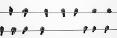
Figure 1: Birds on wires.

Our PB model also resembles random sequential adsorption (RSA) [25, 26, 27, 28, 29, 30, 31, 32, 33], where fixed-shape particles impinge on open regions of a substrate and stick irreversibly. One example of RSA that is close to our PB model is the “unfriendly seating arrangement” problem [34, 35], where people arrive one at a time at a luncheonette and and sit at a counter. People are all mutually unfriendly so they choose seats at random but never next to another person. The luncheonette reaches a static jammed state of density $\rho_{\text{jam}}=\tfrac{1}{2}(1-e^{-2})\approx 0.432$, after which additional patrons cannot be accommodated. In contrast, our PB model reaches a steady state that is constantly changing locally, but its global properties are stationary and independent of the initial conditions.

While our model is couched in terms of birds, it should not be taken literally as a description of real birds. There are many other influences that the determine how birds organize themselves on a spatially restricted landing spot, such as a wire. Nevertheless, the behavior of our admittedly unrealistic model is rich and perhaps this study provides some initial steps to understand the organizational dynamics of more realistic models of the arrival and departure of birds at some resting spot. We view our PB model has being akin to some of the idealized forest-fire models that were proposed long ago in the statistical physics literature [11, 12, 13, 14]. These abstract models miss many features of real forest fires; nevertheless, the phenomenology that arises from this class of models is extremely rich and led to many advances about self-organized criticality [36]. It is in this impressionistic spirit that we investigate our PB model.

2 One-Dimensional Lattice

It is conceptually simplest to formulate a discrete version of our PB model in which birds land on empty sites of a one-dimensional lattice; we later treat a continuous version. Each landing event of a bird scares away birds on adjacent lattice sites (if they are present) so that they fly away. Our analysis of the PB model focuses on $V_{k}$, the density of voids of length $k$. A void of length $k$ is defined as the following arrangement of birds and vacancies

$$\circ\bullet\underbrace{\circ\,\ldots\,\circ}_{k}\bullet\,\circ\,,$$

where an occupied site is denoted by $\bullet$ and an empty site by $\circ$. Since birds cannot be adjacent, the sites next to each bird outside any void must also be empty.

2.1 The void densities

The void densities change in time according to the following rate equations:

$$\dot{V}_{k}=-kV_{k}-2V_{k}+2V_{k-1}+2\sum_{j\geq k+1}V_{j}=-(4+k)V_{k}+2\sum_{j\geq k-1}V_{j}\,,$$ (1)

where the overdot denotes time derivative. Each of the terms on the right corresponds to one of the processes shown in Fig. 2. The first term accounts for the loss of a $k$-void due to a bird landing anywhere within this void (Fig. 2(a)). The second term accounts for the loss of the $k$-void when a bird lands in either of the two sites just outside this void. Immediately afterwards, the adjacent bird at the edge of the $k$-void flies away, so that a $k$-void disappears (Fig. 2(b)). The third term accounts for the gain of a $k$-void when a bird lands on either of the two sites just outside a void of length $k-1$; this ultimately causes an increase in the number of $k$-voids (Fig. 2(c)). The last term accounts for the gain of $k$-voids when a bird lands within a $j$-void, with $j>k$, such that a $k$-void is created. If $j\neq 2k+1$, there are two possible landing sites (Fig. 2(d)), each of which creates one $k$-void. If $j=2k+1$, there is a unique landing site in the middle of the $j$-void that creates two $k$-voids.

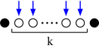
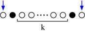
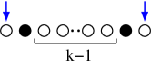
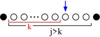
Figure 2: Processes that contribute to changes in the void densities in the PB model of Eq. (1). The vertical arrows indicate the possible locations for a bird to land. In (d) only one of the two possible landing spots that creates a void of length $k$ is shown.

The void distribution also satisfy the following basic conditions that will be useful in solving the model:

$$V_{0}=0\,,\qquad\sum_{k\geq 0}V_{k}=\rho\,,\qquad\sum_{k\geq 0}(k+1)V_{k}=1.$$ (2)

The first equality states that voids of length 0 cannot exist because this corresponds to two birds being adjacent. The one-to-one correspondence between each void and exactly one bird leads to the second equality between void densities $V_{k}$ and the overall density $\rho$. The last equality states that the length of all voids plus the bird at one end of each void equals the total length.

Summing Eqs. (1) over all $k\geq 1$ and using the sum rules (2), we obtain a closed equation for the density, $\dot{\rho}=1-3\rho$. For an initially empty system, the solution is

$$\rho=\frac{1}{3}(1-e^{-3t})\,.$$ (3)

Thus the approach to the steady-state density of $\rho=\frac{1}{3}$ is purely exponential. We now recast Eqs. (1) as

$$\dot{V}_{1} =-5V_{1}+2\rho$$

$$\dot{V}_{2} =-6V_{2}+2\rho$$

$$\dot{V}_{3} =-7V_{3}-2V_{1}+2\rho$$

$$\dot{V}_{4} =-8V_{4}-2V_{1}-2V_{2}+2\rho\,,$$

etc., which we can solve recursively to give

$$\begin{split}V_{1}&=\tfrac{1}{15}\left(2-5e^{-3t}+3e^{-5t}\right)\\ V_{2}&=\tfrac{1}{9}\left(1-e^{-3t}\right)^{2}\\ V_{3}&=\tfrac{1}{35}\left(2-7e^{-5t}+5e^{-7t}\right)\\ V_{4}&=\tfrac{1}{45}\left(1+4e^{-3t}-6e^{-5t}-5e^{-6t}+6e^{-8t}\right)\,,\end{split}$$ (4)

etc., for an initially empty system. Since each void density approaches its steady-state value exponentially quickly, we now focus on the steady state, where Eqs. (1) reduce to

$$(k+4)V_{k}=2\sum_{j\geq k-1}V_{j}\,.$$ (5)

Introducing the cumulative distribution $F_{k}\equiv\sum_{j\geq k}V_{j}$, (5) becomes

$$F_{k+1}-F_{k+2}=\frac{2}{k+5}\,F_{k}\,.$$ (6)

The first two of Eqs. (2) give $F_{0}=F_{1}=\rho=\frac{1}{3}$; these serve as the initial conditions that allow us to generate all the $F_{k}$ one by one: $F_{2}=\frac{1}{5}$, $F_{3}=\frac{4}{45}$, $F_{5}=\frac{2}{63}$, etc.

To find the general solution of Eq. (6) we employ the generating function technique [37]. The factor $(k+5)^{-1}$ on the right-hand side of (6) suggests that it is expedient to define the generating function as

$$F(z)\equiv\sum_{k\geq 0}F_{k}z^{k+4}\,.$$

Multiplying Eq. (6) by $z^{k+5}$ and summing over all $k\geq 0$, we transform the recurrence (6) into the integral equation

$$F(z)-\rho z^{4}-\frac{F(z)-\rho z^{4}-\rho z^{5}}{z}=2\int_{0}^{z}dw\,F(w)\,.$$ (7)

We now define

$$\Phi(z)=\int_{0}^{z}dw\,F(w)=\sum_{k\geq 0}\frac{F_{k}}{k+5}\,z^{k+5}\,,$$

and after some elementary manipulations, we may express (7) as the ordinary differential equation

$$(1-z)\,\frac{d\Phi}{dz}+2z\Phi=\rho z^{4}\,.$$ (8)

Integrating (8) subject to $\Phi(0)=0$ yields

$$\Phi=\rho\,(1-z)^{2}e^{2z}\int_{0}^{z}dw\,\frac{w^{4}\,e^{-2w}}{(1-w)^{3}}=\tfrac{1}{4}\,\rho\big{[}3(1-z)^{2}e^{2z}-3+3z^{2}+2z^{3}\big{]}\,.$$

Finally, we differentiate $\Phi$ to give the generating function

$$F(z)=\tfrac{3}{2}\,\rho\,\big{[}z+z^{2}-z(1-z)e^{2z}\big{]}\,.$$ (9)

We now expand $F(z)$ in a power series to extract the $F_{k}$:

$$F_{k}=2^{k+1}\,\frac{k+1}{(k+3)!}\,,$$

from which the density of voids of length $k$ is

$$V_{k}=F_{k}-F_{k+1}=2^{k+1}\,\frac{k(k+3)}{(k+4)!}\,.$$ (10)

The average void length $\langle k\rangle=\sum kV_{k}/\sum V_{k}=2$, which accords both with $\rho=\frac{1}{3}$ and with the conditions (2). Higher moments of the void length are less simple: $\langle k^{2}\rangle=3e^{2}\!-\!17\approx 5.167$, $\langle k^{3}\rangle=83\!-\!9e^{2}\approx 16.499$, etc.

A basic question about the steady state is: how many birds fly away after each landing event? According to our model definition, either 0, 1, or 2 birds can fly away when a bird lands. The probabilities $q_{n}$ that $n\leq 2$ birds fly away after each landing event satisfy the sum rules

$$q_{0}+q_{1}+q_{2}=1\,,\qquad q_{1}+2q_{2}=1\,.$$

The first equation imposes normalization, while the second equation states that in the steady state one bird flies away, on average, after each landing event. These lead to $q_{0}=q_{2}$. The probabilities $q_{n}$ are determined by

$$q_{0} =\sum_{k\geq 3}\frac{(\!k-\!2)V_{k}}{1\!-\!\rho}\qquad q_{1}=\sum_{k\geq 2}\frac{2V_{k}}{1\!-\!\rho}\qquad q_{2}=\frac{V_{1}}{1\!-\!\rho}\,.$$

The first term accounts for a bird landing in the interior of a gap of length $k\geq 3$ so that no bird leaves. The second term accounts for a bird landing at either end of a gap of length $k>2$ so that a single bird leaves. The last term account for a bird landing in a vacancy between two birds so that both these birds leave. The normalization factor $(1-\rho)^{-1}$ is the probability to land on any vacancy. Using $\rho=\frac{1}{3}$ and Eq. (10), we find $q_{0}=q_{2}=\frac{1}{5}$, $q_{1}=\frac{3}{5}$.

We can also readily extend our approach to treat the situation in which all birds within a range $b>1$ fly away when a bird lands on an unoccupied site. While the qualitative features of this generalization are the same as that for the case $b=1$ given above, some quantitative differences arise. The solution for general $b>1$ is given in A.

3 The pair correlation function

The spatial distribution of birds may be characterized by the pair correlation function $C_{j}\equiv\langle n_{0}n_{j}\rangle$, where $n_{j}$ is the occupancy indicator function at site $j$. That is, $n_{j}=0$ if site $j$ is empty and $n_{j}=1$ if $j$ is occupied. If the locations of the birds are spatially uncorrelated, then $\langle\langle n_{0}n_{j}\rangle=\langle n_{0}\rangle\langle n_{j}\rangle$. This implies that the connected correlation function, $\mathcal{C}_{j}=\langle n_{0}n_{j}\rangle-\langle n_{0}\rangle\langle n_{j}\rangle$ would equal zero. Our calculations below seem to suggest that this is the case. The connected correlation functions $\mathcal{C}_{1}$ and $\mathcal{C}_{2}$ are non zero, while we show that $\mathcal{C}_{4}$, and $\mathcal{C}_{5}$ are zero. These calculations become quite tedious for $\mathcal{C}_{4}$ and $\mathcal{C}_{5}$ and we can only conjecture that $\mathcal{C}_{j}=0$ for $j>5$.

The steady-state pair correlation function $C_{j}$ for $j\leq 3$ can be deduced directly from our results for the density and the void densities. Indeed, $C_{0}=\langle n_{0}^{2}\rangle=\langle n_{0}\rangle=\frac{1}{3}$, while $C_{1}=V_{0}$, $C_{2}=V_{1}$ and $C_{3}=V_{2}$, from which

$$C_{0}=\tfrac{1}{3}\,,\quad C_{1}=0\,,\quad C_{2}=\tfrac{2}{15}\,,\quad C_{3}=\tfrac{1}{9}\,.$$ (11)

We now derive $C_{4}=C_{5}=\frac{1}{9}$. As we show, determining these correlation functions requires various multi-void distributions. The formal expressions for the first few correlation functions $C_{j}$, with $j\geq 4$, are:

$$C_{4} =\text{Prob}\Big{[}\!\bullet\!\circ\!\bullet\!\circ\!\bullet\!\Big{]}+\text{Prob}\Big{[}\!\bullet\!\circ\!\circ\!\circ\!\bullet\!\Big{]}=V_{1,1}+V_{3}$$

$$C_{5} =\text{Prob}\Big{[}\!\bullet\!\circ\!\bullet\!\circ\!\circ\!\bullet\!\Big{]}+\text{Prob}\Big{[}\!\bullet\!\circ\!\circ\!\bullet\!\circ\!\bullet\!\Big{]}+\text{Prob}\Big{[}\!\bullet\!\circ\!\circ\!\circ\!\circ\!\bullet\!\Big{]}=2V_{1,2}+V_{4}$$

$$C_{6} =\text{Prob}\Big{[}\!\bullet\!\circ\!\bullet\!\circ\!\bullet\!\circ\!\bullet\!\Big{]}+\text{Prob}\Big{[}\!\bullet\!\circ\!\circ\!\bullet\!\circ\!\circ\!\bullet\!\Big{]}+\text{Prob}\Big{[}\!\bullet\!\circ\!\bullet\!\circ\!\circ\!\circ\!\bullet\!\Big{]}$$

$$\qquad\qquad+\text{Prob}\Big{[}\!\bullet\!\circ\!\circ\!\circ\!\bullet\!\circ\!\bullet\!\Big{]}+\text{Prob}\Big{[}\!\bullet\!\circ\!\circ\!\circ\!\circ\!\circ\!\bullet\!\Big{]}$$

$$=V_{1,1,1}+V_{2,2}+2V_{1,3}+V_{5}\,,$$

where

$$V_{k}\equiv\text{Prob}\Big{[}\bullet\underbrace{\circ\,\ldots\,\circ}_{k}\bullet\Big{]}$$

$$V_{i,j}\equiv\text{Prob}\Big{[}\bullet\underbrace{\circ\,\ldots\,\circ}_{i}\bullet\underbrace{\circ\,\ldots\,\circ}_{j}\bullet\Big{]}$$

$$V_{i,j,k}\equiv\text{Prob}\Big{[}\bullet\underbrace{\circ\,\ldots\,\circ}_{i}\bullet\underbrace{\circ\,\ldots\,\circ}_{j}\bullet\underbrace{\circ\,\ldots\,\circ}_{k}\bullet\Big{]}\,,$$

denote the single-void, two-void, and three-void distributions. The subscripts on the multi-void distributions account for the number of sites in the adjacent empty strings.

The void distributions $V_{i_{1},\ldots,i_{p}}$ satisfy rate equations that are natural extensions of the rate equation (1) for $V_{k}$. Consider first the distribution $V_{i,j}$. Using the same reasoning as that given in Fig. 2 to write Eq. (1), the rate equation for $V_{i,j}$ is

$$\dot{V}_{i,j} =-(2+i+j)V_{i,j}+\sum_{\ell\geq i+1}V_{\ell,j}+\sum_{\ell\geq j+1}V_{i,\ell}$$

$$\qquad\qquad+V_{i+j+1}+V_{i-1,j+1}+V_{i+1,j-1}+V_{i-1,j}+V_{i,j-1}\,,$$ (12)

subject to the boundary conditions

$$V_{i,0}=0=V_{0,j}\qquad(i,j\geq 0),$$ (13)

and the sum rules

$$\sum_{\ell\geq 1}V_{\ell,j}=V_{j},\qquad\sum_{\ell\geq 1}V_{i,\ell}=V_{i}\,.$$ (14)

In the steady state, (3) reduces to the recurrence

$$(4+i+j)V_{i,j}=\sum_{\ell\geq i}V_{\ell,j}+\sum_{\ell\geq j}V_{i,\ell}+V_{i+j+1}+V_{i-1,j+1}+V_{i+1,j-1}+V_{i-1,j}+V_{i,j-1}\,.$$ (15)

Specializing (15) and (14) to $(i,j)=(1,1)$ and additionally using (13) we obtain

$$6V_{1,1}=2V_{1}+V_{3}\,.$$ (16)

Recalling that $V_{1}=\frac{2}{15}$ and $V_{3}=\frac{2}{35}$ from Eq. (10), we obtain $V_{1,1}=\frac{17}{315}$, which finally gives $C_{4}=V_{1,1}+V_{3}=\frac{1}{9}$.

Next, we specialize (15) and (14) to $(i,j)=(1,2)$, from which we obtain

$$6V_{1,2}=V_{2}+V_{1}+V_{4}$$ (17)

Using the known results $V_{1}=\frac{2}{15},V_{2}=\frac{1}{9},V_{4}=\frac{1}{45}$ we obtain $V_{1,2}=\frac{2}{45}$ and then $C_{5}=2V_{1,2}+V_{4}=\frac{1}{9}$.

We mention that we can determine the full time dependence of the low-order pair correlation functions. The behaviors of $C_{j}$ with $j=0,1,2$, and 3 follow directly from the relation between these correlation functions and the appropriate void densities. Namely, $C_{0}(t)=\rho(t)$, $C_{1}(t)=V_{0}(t)$, $C_{2}(t)=V_{1}(t)$ and $C_{3}(t)=V_{2}(t)$. To derive $C_{4}(t)=V_{1,1}(t)+V_{3}(t)$ we must find $V_{1,1}(t)$. From (3) The rate equation for $V_{1,1}$ is

$$\dot{V}_{1,1}=-6V_{1,1}+2V_{1}+V_{3}\,,$$

with solution, for an initially empty system,

$$V_{1,1}=\tfrac{1}{315}\left(17-70e^{-3t}+63e^{-5t}+35e^{-6t}-45e^{-7t}\right)\,.$$ (18)

Using $C_{4}=V_{1,1}+V_{3}$ with $V_{3}(t)$ from (4) and $V_{1,1}(t)$ from (18) we have

$$C_{4}=V_{1,1}+V_{3}=\tfrac{1}{9}\left(1-e^{-3t}\right)^{2}\\$$ (19)

To derive (21), we must find $V_{1,2}(t)$. Again from (3), the rate equation for $V_{1,2}$ is

$$\dot{V}_{1,2}=-6V_{1,2}+V_{1}+V_{2}+V_{4}\,,$$

whose solution is

$$V_{1,2}=\tfrac{1}{45}\left(2-7e^{-3t}+3e^{-5t}+5e^{-6t}-3e^{-8t}\right)\,.$$ (20)

Using $C_{5}=2V_{1,2}+V_{4}$ with $V_{4}(t)$ from (4) and $V_{1,2}(t)$ from (20) we thus find

$$C_{5}=2V_{1,2}+V_{4}=\tfrac{1}{9}\left(1-e^{-3t}\right)^{2}\,.$$ (21)

It seems unlikely that we can determine of the correlation functions $C_{j}$ for arbitrary $j$ via this straightforward, but laborious method.

4 One-dimensional continuum

A more natural scenario for the dynamics is that each birds can land anywhere along a wire. Within the RSA framework, the analogous process is the famous Rényi car parking model [38] in which fixed-length cars attempt to park anywhere along a one-dimensional line until there are no gaps remaining that can accommodate a car. Without loss of generality we set the interaction range between birds equal to one. Thus if a bird lands within a unit distance of one (or two) birds, this bird (or these birds) immediately fly away.

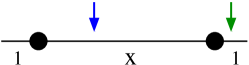
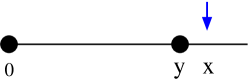
Figure 3: Processes that contribute to changes in the void densities in Eq. 22. (a) An $x$-void disappears if a bird lands anywhere inside the void (blue arrow) or within a unit distance of either bird outside the void (green arrow), (b) An $x$-void is created when a new bird lands a distance $x$ from an existing bird. Another bird may be anywhere in the range $[1,\infty]$ for $1<x<2$ or in the range $[x-1,\infty]$ for $x>2$.

Instead of voids of integer length, the basic dynamical variable is $V(x)$, the density of voids of length $x$. Following the same reasoning as that which led to Eq. (1), the evolution equation for the void distribution is now (see also Fig. 3)

$$\dot{V}(x,t)=-(2+x)V(x,t)+\begin{cases}{\displaystyle 2\int_{1}^{\infty}dy\,V(y,t)}&\qquad\qquad 1<x<2\,,\\[14.22636pt] {\displaystyle 2\int_{x-1}^{\infty}dy\,V(y,t)}&\qquad\qquad x>2\,.\end{cases}$$ (22)

In close analogy with Eq. (2), the void distribution $V(x)$ must now satisfy the sum rules: (a) $V(x)=0$ for $x<1$, (b) the density of birds is $\rho=\int_{1}^{\infty}dx\,V(x)$, and (c) $\int_{1}^{\infty}dx\,x\,V(x)=1$. As a result of condition (b), the first of Eqs. (22) can be re-expressed as $\dot{V}(x,t)=-(2+x)V(x,t)+2\rho(t)$.

Integrating (22) over all $x$, the density

$$\rho(t)=\int_{1}^{2}dx\,V(x,t)+\int_{2}^{\infty}dx\,V(x,t)$$

obeys the rate equation $\dot{\rho}=1-2\rho$. For an initially empty system, the solution is simply $\rho=\frac{1}{2}(1-e^{-2t})$. We now use this result $\rho$ to solve $\dot{V}(x,t)=-(2+x)V(x,t)+2\rho(t)$ in the range $1<x<2$ to give

$$V(x,t)=\frac{1-e^{-(2+x)t}}{2+x}-\frac{e^{-2t}-e^{-(2+x)t}}{x}\,.$$ (23)

Using $\rho=\frac{1}{2}(1-e^{-2t})$ in the second of (22), we may rewrite this equation as

$$\dot{V}(x,t)=-(2+x)V(x,t)-2\int_{1}^{x-1}dy\,V(y,t)+1-e^{-2t}\,.$$ (24)

We now substitute the solution for $V(x,t)$ in the range $1<x<2$ in Eq. (24) to solve this equation in the interval $2<x<3$. Continuing this procedure we can recursively solve (24) for each interval $n<x<n+1$ using the previously determined solutions for $x<n$. While this procedure is straightforward in principle, it quickly becomes tedious as $x$ increases.

To obtain the large-$x$ behavior of the void distribution, we first rely on the fact that the approach to the steady state again occurs exponentially quickly. Thus we henceforth focus on the steady-state properties of the continuum case. In this case, the void density is determined by

$$(2+x)V(x)=\begin{cases}{\displaystyle 2\int_{1}^{\infty}dy\,V(y)}&\qquad\qquad x<1\,,\\[14.22636pt] {\displaystyle 2\int_{x-1}^{\infty}dy\,V(y)}&\qquad\qquad 1<x<2\,.\end{cases}$$ (25)

To solve Eq. (25), we introduce the Laplace transform $\widehat{V}(s)\equiv\int_{1}^{\infty}dx\,e^{-xs}\,V(x)$. Then the Laplace transform of the left-hand side of Eq. (25) is

$$\int_{1}^{\infty}dx\,e^{-xs}(2+x)V(x)=2\widehat{V}-\frac{d\widehat{V}}{ds}\,.$$

The Laplace transform of the right-hand side of the first of (25) is, after accounting for the constraint $1<x<2$,

$$2\rho\int_{1}^{2}dx\,e^{-xs}=\frac{2\rho}{s}\,(e^{-s}-e^{-2s})\,.$$

Similarly, the Laplace transform of the right-hand side of the second of (25) is, after accounting for the constraint $x>2$,

$$\int_{2}^{\infty}\!dx\,e^{-xs}\int_{x-1}^{\infty}dy\,V(y)=\int_{1}^{\infty}\!\!\!dy\,V(y)\int_{2}^{y+1}\!\!dx\,e^{-xs}=\frac{e^{-s}}{s}\,\left(\rho e^{-s}-\widehat{V}\right)\,.$$

Using these results, the Laplace transform satisfies

$$2\left(1+s^{-1}e^{-s}\right)\widehat{V}-\frac{d\widehat{V}}{ds}=2\rho s^{-1}e^{-s}\,.$$ (26)

Integrating (26) and using the steady-state density $\rho=\frac{1}{2}$ yields

$$\widehat{V}(s)=\frac{1}{2}-\mathcal{E}(s)\int_{s}^{\infty}\frac{d\sigma}{\mathcal{E}(\sigma)}\,.$$ (27)

where we define $\mathcal{E}(s)\equiv e^{2s-2E_{1}(s)}$ and $E_{1}$ is the exponential integral [39]

$$E_{1}(s)=\int_{s}^{\infty}\frac{d\sigma}{\sigma}\,e^{-\sigma}\,.$$

The large-$x$ behavior of $V(x)$ is in principle encoded in the Laplace transform $\widehat{V}(s)$. However, it is easier to extract the asymptotic behavior from the derivative of Eq. (25), namely, from

$$[(2+x)V(x)]^{\prime}=-2V(x-1)\,,$$ (28)

where the prime denotes differentiation with respect to $x$. We will find that $V(x)$ decays super-exponentially with $x$ for large $x$. Thus a Taylor expansion of $V(x)$ is not justified. Instead we seek a solution of the form $V(x)=e^{-w(x)}$, where it is justifiable to expand $w(x-1)$ as $w(x)-w^{\prime}(x)$. Doing so in Eq. (28) gives $xw^{\prime}=2e^{w^{\prime}}$ to leading order. The solution to this equation is

$$w=x[\ln x+\ln(\ln x)-1-\ln 2]+\ldots\,.$$ (29)

Thus the void density $V(x)=e^{-w(x)}$ exhibits essentially a factorial (faster than exponential) decay.

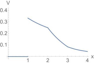
Figure 4: The void density $V(x)$ for $0<x<4$, showing the jump at $x=1$ and singularities in the first derivative at $x=2$ and $x=3$.

We can use the result $\rho=\frac{1}{2}$ to directly find $V(x)$ in the successive intervals $1<x<2$, $2<x<3$, etc., from (25) without recourse to the Laplace transform method. From the first of (25), we obtain

$$V(x)=\begin{cases}\displaystyle{\frac{1}{2+x}}&1<x<2\,,\\[22.76219pt] \displaystyle{\frac{\left[1-2\ln\left((x+1)/3\right)\right]}{2+x}}&2<x<3\,.\end{cases}$$ (30)

For $x>2$, we recast the first of Eqs. (25) into

$$(2+x)V(x)=1-2\int_{1}^{x-1}dy\,V(y)\,,$$ (31)

from which the density, for $3<x<4$, is

$$(2+x)V(x)=1-\ln(4/9)-2\text{Li}_{2}(-3)+2\text{Li}_{2}(-x)-(1+2\ln 3-2\ln x)\ln(1+x)\,,$$

where $\text{Li}_{2}(-x)=\sum_{j\geq 1}(-x)^{j}/j^{2}$ is the dilogarithm function [39]. One may continue this iterative procedure to obtain explicit expressions for $V(x)$ for $n<x<n+1$ for positive integer $n$. These calculations quickly become tedious, so we do not extend them beyond $x=4$. The resulting function $V(x)$ is singular (Fig. 4) with a slope discontinuity at every integer $x\geq 2$; thus inversion of the Laplace transform (27) in terms of a compact formula is also not possible. The main features of the void distribution $V(x)$ is that it is a piecewise smooth function, with increasingly cumbersome expressions for $V(x)$ for $n<x<n+1$, and which decays as $x^{-x}$ for large $x$.

In analogy to the argument that led to the probabilities $q_{n}$ for $n$ birds to fly away at each landing event in the lattice model, in the 1d continuum version the corresponding probabilities are

$$\begin{split}q_{0}&=\int_{2}^{\infty}dx\,(x-2)V(x)\\ q_{1}&=2\int_{2}^{\infty}dx\,V(x)+2\int_{1}^{2}dx\,(x-1)V(x)\\ q_{2}&=\int_{1}^{2}dx\,(2-x)V(x)\end{split}$$ (32)

Using $\rho=\frac{1}{2}$ and (30) we find $q_{0}=q_{2}=4\ln(4/3)-1\approx 0.151$ and $q_{1}=3-8\ln(4/3)\approx 0.699$.

5 Higher dimensions

Our PB model naturally extends to the realistic situation of multiple wires, as in Fig. 1, and to higher dimensions. On hyper-cubic lattices $\mathbb{Z}^{d}$, we posit that all resting birds that are one lattice spacing from the newly arriving bird fly away. In the continuum $\mathbb{R}^{d}$, all resting birds within a unit distance of the newly arriving bird fly away. Simulations of the PB model on various substrates show that an initially empty system quickly reaches a steady state, and the steady-state densities are $\rho\approx\frac{1}{5}$ and $\rho\approx\frac{1}{7}$, respectively, for the square and cubic lattices. These results lead to conjectural steady-state densities on $d$-dimensional hyper-cubic lattices

$$\rho=\frac{1}{2d+1}\,.$$ (33)

The derivation of this result is left to future work.

It is also instructive to construct a mean-field theory for the steady-state density of the PB model on hypercubic lattices. This theory is based on neglecting correlations in the spatial positions of the birds. In this approximation, the density of birds on a $d$-dimensional hypercubic lattice obeys the rate equation

$$\frac{d\rho}{dt}=-(1-\rho)\sum_{n=0}^{2d}(n-1)\binom{2d}{n}(1-\rho)^{2d-n}\rho^{n}\,.$$ (34)

The $n=0$ term in this sum is positive corresponds to the case where the bird lands on an empty site and all neighbors of this site are also empty, so that no birds fly away and $\rho$ increases. The terms with $n\geq 1$ are non-negative and correspond to the situations where at least one resting bird flies away when the bird lands. Equation (34) simplifies to $\frac{d\rho}{dt}=(1-\rho)(1-2\rho\,d)$. This gives the steady-state density $\rho=\frac{1}{2d}$, which approaches the exact steady state (33) in the limit $d\to\infty$. From this same mean-field argument, the probabilities $q_{n}$ for $n$ birds to fly away, with $0\leq n\leq 2d$, after each landing event is

$$q_{n}=\binom{2d}{n}(1-\rho)^{2d-n}\rho^{n}\,.$$ (35)

Using the mean-field steady-state density $\rho=\frac{1}{2d}$, the above expression reduces to $q_{n}=e^{-1}/n!$ as $d\to\infty$. This is a rapidly decaying distribution, so that the average size of the “avalanche” that is nucleated when a bird lands is small: $\langle n\rangle=1-e^{-1}$.

6 Concluding comments

Our PB model is inspired by natural observations and seamlessly leads to a simple non-equilibrium statistical physics model of competing adsorption/desorption. We solved for the time-dependent and steady-state properties of the model analytically. An appealing challenge is to determine the steady-state properties of the PB model in general dimensions, both on lattices and on a continuum. Another potentially fruitful direction is to extend to realistic longer-range interactions between birds. In such a scenario, when a bird lands, it may drive a large groups of birds to fly away. This type of slow driving and sudden large “avalanches” is reminiscent of the size of fires in self-organized forest fire models [12, 13], as well as the size of mass rearrangements in the random organization model [40, 41].

Appendix A Birds with Interaction Range $b>1$

We outline some basic steady-state properties of our PB model on a discrete one-dimensional lattice in which, after each landing event, all birds that are within a distance $b$ of the incident bird fly away. While the solution for the generating function can again be obtained by following the steps from Eqs. (5)–(9), this calculation becomes cumbersome as $b$ increases. However, the steady-state density $\rho=1/(2b+1)$ can be extracted fairly easily without the complete solution for the void distribution.

Let us first treat the case $b=2$; the extension for $b>2$ then readily follows. In the steady state, the generalization of Eq. (5) for the void densities $V_{k}$ is

$$(k+6)V_{k}=2\sum_{j\geq k-2}V_{j}=2F_{k-2}\,.$$ (36)

We use the initial conditions $V_{0}=V_{1}=0$, as well as $\rho=\sum_{k\geq 0}V_{k}$ to solve (36) recursively and obtain

$$V_{2}=\tfrac{1}{4}\rho,\qquad V_{3}=\tfrac{2}{9}\rho,\qquad V_{4}=\tfrac{1}{5}\rho,\qquad V_{5}=\tfrac{3}{22}\rho\,,$$ (37)

etc. By using the generating function technique, we can fix $\rho$ and then determine $V_{k}$ for arbitrary $k$. However, if we merely want to find the steady-state density, we adopt the following approach. We first rewrite (36) as

$$(k+8)[F_{k+2}-F_{k+3}]=2F_{k}\,,$$ (38)

and then sum over all $k\geq 0$ to yield

$$7F_{2}+\sum_{k\geq 2}F_{k}=2\sum_{k\geq 0}F_{k}\,.$$ (39)

The initial conditions $V_{0}=V_{1}=0$ leads to $F_{0}=F_{1}=F_{2}=\rho$, which then allows us to reduce (39) to

$$5\rho=\sum_{k\geq 0}F_{k}\,.$$ (40)

Using the normalization condition $\sum_{k\geq 0}(k+1)V_{k}=\sum_{k\geq 0}F_{k}=1$ we arrive at the basic result

$$\rho=\frac{1}{5}\,.$$ (41)

We now determine the probabilities $q_{n}$ that $n$ birds fly away after each landing event. First note that $q_{2}$ is given by

$$q_{2}=\tfrac{5}{4}\left(2V_{2}+V_{3}\right)\,.$$ (42)

The factor $\frac{5}{4}$ accounts for that fact that the fraction of successful landing events in the steady state is $\frac{4}{5}$. The term $2V_{2}$ accounts for the 2 landing spots inside a vacancy of length 2 that leads to two birds flying away, while the term $V_{3}$ accounts for the fact that the landing must be at the center of a gap of length 3 to trigger two departures. Using (37) and (41), the remaining probabilities $q_{n}$ are

$$q_{0}=q_{2}=\frac{13}{72}\,,\qquad q_{1}=\frac{23}{36}\,.$$ (43)

For the case of arbitrary $b$. The analog of Eq. (38) is

$$(k+3b+2)[F_{k+b}-F_{k+b+1}]=2F_{k}\,.$$ (44)

Summing over all $k\geq 0$ we obtain

$$(3b+1)F_{b}+\sum_{k\geq b}F_{k}=2\sum_{k\geq 0}F_{k}$$ (45)

The initial condition $F_{0}=F_{1}=\ldots=F_{b}=\rho$ yields $\sum_{k\geq b}F_{k}=\sum_{k\geq 0}F_{k}+b\rho$. Using this in (45), we obtain

$$(2b+1)\rho=\sum_{k\geq 0}F_{k}\,.$$ (46)

Now using the normalization condition $\sum_{k\geq 0}F_{k}=1$, the steady-state density is

$$\rho=\frac{1}{2b+1}\,.$$ (47)

From (44) and (47), and using the initial condition $F_{j}=\rho$ for $j\leq b$ as well as the definition of $V_{k}$ in terms of $F_{k}$, we find

$$V_{b+j}=\frac{2}{2b+1}\,\frac{1}{3b+2+j}\,.$$ (48)

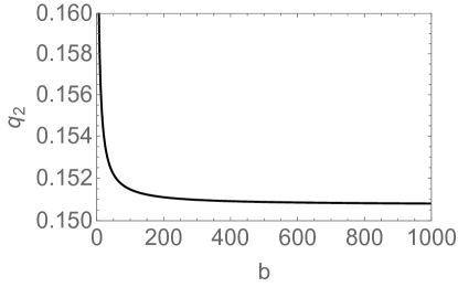
Figure 5: The probability $q_{2}$ as a function of $b$ for $b\leq 1000$.

Let us now determine the probabilities $q_{n}$ for arbitrary $b$. The generalization of (42) is

$$q_{2}=\frac{2b+1}{2b}\sum_{j=0}^{b}(b-j)V_{b+j}\,.$$ (49)

The meaning of each term in the sum is the same as the two terms in Eq. (42): we are counting the number of ways that a bird can land within a gap of length $b+j$ such that exactly two birds fly away. Substituting in (48) into (49) and computing the sum, we obtain

$$q_{2}=2(2+b^{-1})(H_{4b+2}-H_{3b+1})-1-b^{-1}\,,$$ (50)

where $H_{n}=\sum_{1\leq j\leq n}j^{-1}$ is the $n^{\rm th}$ harmonic number. Again, $q_{0}=q_{2}$ and $q_{1}$ is fixed by normalization, $q_{1}=1-2q_{2}$. For $b\to\infty$, $q_{2}\to 4\ln(4/3)-1\approx 0.15073$, which reproduces the continuum result of Eq. (32), as it must. The dependence of $q_{2}$ on $b$ is shown in Fig. 5.

Now we extend the above result to find the time-dependent behavior. For general $b>1$, the void densities $V_{k}$ with $k\geq b$ evolve according to

$$\dot{V}_{k}=-(2b+2+k)V_{k}+2\sum_{\ell\geq k-b}V_{\ell}\,,$$ (51)

subject to the constraint that $V_{0}=\ldots=V_{b-1}=0$. Summing Eqs. (51) over $k\geq b$ and using the above constraint, as well as Eqs. (2), we obtain the simple equation for the density

$$\dot{\rho}=1-(2b+1)\rho\,,$$

from which

$$\rho(t)=\frac{1-e^{-(2b+1)t}}{2b+1}\,.$$ (52)

The first non-trivial void density $V_{b}$ satisfies

$$\dot{V}_{b}(t)=-(3b+2)V_{b}+2\rho\,,$$ (53)

from which

$$V_{b}=\frac{2}{(2b+1)(3b+2)}-\frac{2\;e^{-(2b+1)t}}{(b+1)(2b+1)}+\frac{2\;e^{-(3b+2)t}}{(b+1)(3b+2)}\,.$$ (54)

The density $V_{b+1}$ satisfies

$$\dot{V}_{b+1}=-(3b+3)V_{b+1}+2\rho\,,$$ (55)

from which

$$V_{b+1}(t)=\frac{2}{(2b+1)(3b+3)}-\frac{2\;e^{-(2b+1)t}}{(b+2)(2b+1)}+\frac{2\;e^{-(3b+3)t}}{(b+2)(3b+3)}\,.$$ (56)

When $b\leq k\leq 2b$, the rate equation for $V_{k}$ has a form

$$\dot{V}_{k}=-(2b+2+k)V_{b+j}+2\rho$$ (57)

similar to (53) and (55). Solving (57) yields

$$V_{k}=\frac{2}{(2b+1)(2b+2+k)}-\frac{2\;e^{-(2b+1)t}}{(k+1)(2b+1)}+\frac{2\,e^{-(2b+2+k)t}}{(k+1)(2b+2+k)}$$ (58)

for $b\leq k\leq 2b$.

Appendix B Higher-Order Correlation Functions

The pattern in the equations for $C_{4}$, $C_{5}$, and $C_{6}$ generalizes in straightforward way and we merely write the equations for the next three correlation functions in the steady state:

$$C_{7} =2V_{1,1,2}+V_{1,2,1}+2V_{1,4}+2V_{2,3}+V_{6}$$

$$C_{8} =V_{1,1,1,1}+2V_{1,1,3}+V_{1,3,1}+2V_{1,5}+2V_{2,4}+V_{3,3}+V_{7}$$

$$C_{9} =2V_{1,1,1,2}+2V_{1,1,2,1}+2V_{1,1,4}+V_{1,4,1}+2V_{2,1,3}+2V_{1,2,3}+2V_{1,3,2}+V_{2,2,2}$$

$$\qquad\qquad+2V_{1,6}+2V_{2,5}+2V_{3,4}+V_{8}\,.$$

References

- [1] Vicsek T, Czirók A, Ben-Jacob E, Cohen I and Shochet O 1995 Phys. Rev. Lett. 75(6) 1226–1229 URL https://link.aps.org/doi/10.1103/PhysRevLett.75.1226
- [2] Toner J and Tu Y 1995 Phys. Rev. Lett. 75(23) 4326–4329 URL https://link.aps.org/doi/10.1103/PhysRevLett.75.4326
- [3] Toner J and Tu Y 1998 Phys. Rev. E 58(4) 4828–4858 URL https://link.aps.org/doi/10.1103/PhysRevE.58.4828
- [4] Couzin I D, Krause J, James R, Ruxton G D and Franks N R 2002 Journal of Theoretical Biology 218 1–11 ISSN 0022-5193 URL https://www.sciencedirect.com/science/article/pii/S0022519302930651
- [5] Couzin I D, Krause J, Franks N R and Levin S A 2005 Nature 433 513–516
- [6] Ballerini M, Cabibbo N, Candelier R, Cavagna A, Cisbani E, Giardina I, Lecomte V, Orlandi A, Parisi G, Procaccini A, Viale M and Zdravkovic V 2008 Proceedings of the National Academy of Sciences 105 1232–1237 (Preprint https://www.pnas.org/doi/pdf/10.1073/pnas.0711437105) URL https://www.pnas.org/doi/abs/10.1073/pnas.0711437105
- [7] Ballerini M, Cabibbo N, Candelier R, Cavagna A, Cisbani E, Giardina I, Orlandi A, Parisi G, Procaccini A, Viale M and Zdravkovic V 2008 Animal Behaviour 76 201–215 ISSN 0003-3472 URL https://www.sciencedirect.com/science/article/pii/S0003347208001176
- [8] Vicsek T and Zafeiris A 2012 Physics Reports 517 71–140 ISSN 0370-1573 collective motion URL https://www.sciencedirect.com/science/article/pii/S0370157312000968
- [9] Šeba P 2009 Journal of Statistical Mechanics: Theory and Experiment 2009 L10002 URL https://doi.org/10.1088/1742-5468/2009/10/l10002
- [10] Aydoğdu A, Frasca P, D’Apice C, Manzo R, Thornton J, Gachomo B, Wilson T, Cheung B, Tariq U, Saidel W and Piccoli B 2017 Journal of Theoretical Biology 415 102–112 ISSN 0022-5193 URL https://www.sciencedirect.com/science/article/pii/S0022519316304064
- [11] Bak P, Chen K and Tang C 1990 Physics Letters A 147 297–300 ISSN 0375-9601 URL https://www.sciencedirect.com/science/article/pii/037596019090451S
- [12] Drossel B and Schwabl F 1992 Phys. Rev. Lett. 69(11) 1629–1632 URL https://link.aps.org/doi/10.1103/PhysRevLett.69.1629
- [13] Drossel B, Clar S and Schwabl F 1993 Phys. Rev. Lett. 71(23) 3739–3742 URL https://link.aps.org/doi/10.1103/PhysRevLett.71.3739
- [14] Paczuski M and Bak P 1993 Phys. Rev. E 48(5) R3214–R3216 URL https://link.aps.org/doi/10.1103/PhysRevE.48.R3214
- [15] Grassberger P 2002 New J. Phys. 4 17 URL https://doi.org/10.1088/1367-2630/4/1/317
- [16] Palmieri L and Jensen H J 2020 Frontiers in Physics 8 257 URL https://www.frontiersin.org/article/10.3389/fphy.2020.00257
- [17] Rogers C A 1964 Packing and Covering (Cambridge, UK: Cambridge University Press)
- [18] Levenshtein V I 1979 Dokl. Akad. Nauk SSSR 245 1299–1303 URL http://mi.mathnet.ru/eng/dan/v245/i6/p1299
- [19] Odlyzko A M and Sloane N J A 1979 J. Combin. Theory A 26 210–214 URL https://www.sciencedirect.com/science/article/pii/0097316579900748
- [20] Conway J H and Sloane N J A 1999 Sphere Packings, Lattices and Groups (New York: Springer-Verlag) URL https://doi.org/10.1007/978-1-4757-6568-7
- [21] Hales T C 2005 Ann. Math. 168 1065–1185 URL https://doi.org/10.4007/annals.2005.168.1065
- [22] Aste T and Weaire D 2008 The Pursuit of Perfect Packing (New York: Taylor & Francis)
- [23] Cohn H 2016 arXiv:1603.05202 URL https://doi.org/10.48550/arXiv:1603.05202
- [24] Cohn H 2017 Notices Amer. Math. Soc. 64(2) 102–115 URL https://doi.org/10.1090/noti1474
- [25] Flory P J 1939 J. Amer. Chem. Soc. 61 1518–1521 URL https://doi.org/10.1021/ja01875a053
- [26] Evans J W 1993 Rev. Mod. Phys. 65(4) 1281–1329 URL https://link.aps.org/doi/10.1103/RevModPhys.65.1281
- [27] Talbot J, Tarjus G, Van Tassel P and Viot P 2000 Colloids and Surfaces A: Physicochemical and Engineering Aspects 165 287–324 ISSN 0927-7757 URL https://www.sciencedirect.com/science/article/pii/S0927775799004094
- [28] Torquato S and Haslach HW J 2002 Applied Mechanics Reviews 55 B62–B63 ISSN 0003-6900 (Preprint https://asmedigitalcollection.asme.org/appliedmechanicsreviews/article-pdf/55/4/B62/5439035/b61_1.pdf) URL https://doi.org/10.1115/1.1483342
- [29] Adamczyk Z 2017 Particles at Interfaces: Interactions, Deposition, Structure (Elsevier)
- [30] Krapivsky P L, Redner S and Ben-Naim E 2010 A Kinetic View of Statistical Physics (Cambridge, UK: Cambridge University Press) URL https://doi.org/10.1017/CBO9780511780516
- [31] Sikirić M D and Itoh Y 2011 Random Sequential Packing of Cubes (WORLD SCIENTIFIC) (Preprint https://www.worldscientific.com/doi/pdf/10.1142/7777) URL https://www.worldscientific.com/doi/abs/10.1142/7777
- [32] Bressloff P C and Newby J M 2013 Rev. Mod. Phys. 85(1) 135–196 URL https://link.aps.org/doi/10.1103/RevModPhys.85.135
- [33] Krapivsky P L 2020 Phys. Rev. E 102(6) 062108 URL https://link.aps.org/doi/10.1103/PhysRevE.102.062108
- [34] Freedman D and Shepp L 1962 SIAM Review 4 150 URL https://doi.org/10.1137/1004037
- [35] Friedman H D 1964 SIAM Rev. 6 180–182 ISSN 0036-1445 URL https://doi.org/10.1137/1006044
- [36] Bak P, Tang C and Wiesenfeld K 1987 Phys. Rev. Lett. 59(4) 381–384 URL https://link.aps.org/doi/10.1103/PhysRevLett.59.381
- [37] Wilf H S 2005 generatingfunctionology (CRC press)
- [38] Rényi A 1958 Publ. Math. Inst. Hung. Acad. Sci. 3 109–127
- [39] Abramowitz M and Stegun I A 1964 Handbook of Mathematical Functions with Formulas, Graphs, and Mathematical Tables vol 55 (US Government printing office)
- [40] Wilken S, Guerra R E, Levine D and Chaikin P M 2021 Phys. Rev. Lett. 127(3) 038002 URL https://link.aps.org/doi/10.1103/PhysRevLett.127.038002
- [41] Corte L, Chaikin P M, Gollub J P and Pine D J 2008 Nature Physics 4 420–424