Accurate modelling of extragalactic microlensing by compact objects

Abstract

Microlensing of extragalactic sources, in particular the probability of significant amplifications, is a potentially powerful probe of the abundance of compact objects outside the halo of the Milky Way. Accurate experimental constraints require an equally accurate theoretical model for the amplification statistics produced by such a population. In this article, we argue that the simplest (strongest-lens) model does not meet this demanding requirement. We thus propose an elaborate practical modelling scheme for extragalactic microlensing. We derive from first principles an expression for the amplification probability that consistently allows for: (i) the coupling between microlenses; (ii) realistic perturbations from the cosmic large-scale structure; (iii) extended-source corrections. An important conclusion is that the external shear applied on the dominant microlens, both by the other lenses and by the large-scale structure, is practically negligible. Yet, the predictions of our approach can still differ by a factor of a few with respect to existing models of the literature. Updated constraints on the abundance of compact objects accounting for such discrepancies may be required.

1 Introduction

Needless to say the nature of the dark matter (DM) is one of the most open questions in modern science. Since the first detection of a gravitational-wave signal reported by the LIGO/Virgo Collaboration [1], an old DM candidate got back under spotlight, namely primordial black holes (PBHs) [2, 3, 4]. Originally considered by Zel’dovich & Novikov [5] and Hawking [6], PBHs are to date the only known example of massive compact halo object (MACHO) [7] that could make up a significant fraction of the DM (see e.g. ref. [8] and references therein). Other historical MACHO candidates, such as neutron stars, planets or brown dwarfs, are excluded by a variety of cosmological constraints implying that DM must be non-baryonic; those notably include the precision measurement of the CMB acoustic peaks and the abundance of light elements predicted in the context of the hot big-bang nucleosynthesis – see e.g. chapters 6–8 of ref. [9] for a detailed historical review.

A suitable probe of the clumpiness of the DM is gravitational lensing, which has the virtue of being directly sensitive to the distribution of mass, as opposed to the astronomical observations which rely on luminous matter. In particular, microlensing is found to be a useful tool to detect compact objects. The idea is that, as a compact object crosses the line of sight of a distance source, it temporarily magnifies its apparent brightness [10]. This idea was put into practice by the MACHO experiment [11], which looked for microlensing events in the Magellanic Clouds for several years in the 90s by monitoring thousands of stars hoping that some compact objects in the mass range $3\times 10^{-4}$ to $0.06\,M_{\odot}$ would cross the line of sight and amplify their brightness. Among the 9.5 million light curves that were analysed, only 3 events consistent with microlensing were found. After similar analyses were conducted by the EROS and OGLE collaborations [12, 13], the possibility that the dark halo of our galaxy is made of compact objects in that mass range was excluded. Those constraints keep being discussed in the literature; for instance ref. [14] argues that detection method presented inconsistencies; ref. [15] suggests that the constraints may be alleviated if the compact objects are clustered. Importantly, galactic microlensing is inefficient at detecting high-mass compact objects [16].

Press and Gunn [17] proposed to use quasar microlensing for detecting a cosmologically significant density of compact bodies. This idea was further investigated by Hawkins [18, 19] and Hawkins and Verón [20] who studied the structure of DM using quasar light curves, and Schneider [21], who constrained the population of compact objects that could make up the total matter density. The difficulty of constraining the abundance of high-mass compact objects in our galactic halo motivated the observation of microlensing effects in images of multiple imaged quasars [22, 23, 24]. Microlensing can also manifest as flux ratio anomalies between multiple quasar images [25, 26, 27], which may be interpreted as a direct proof for the presence of CDM substructure around lensing galaxies.

Another method to constrain compact DM, motivated by the recent discoveries of the highly magnified stars MACS J1149 Lensed Star 1 (“Icarus”) [28] and WHL0137-LS (“Earendel”) [29], both visible at cosmological distances, uses caustic-crossing events in giant arcs. This mechanism allows the detection of compact objects in the subsolar-mass regime.

One possible alternative to detect extragalactic microlensing due to compact objects beyond the solar mass is via supernova (SN) lensing. Refdsal [30] was the first to study the possibility of observing this phenomenon and use SNe as a cosmological probe. Since then there has been many research programmes looking for strong gravitational lensing of SNe [31], where microlensing is a potentially worrisome source of noise. The idea of using SN microlensing as a signal, to constrain the abundance of compact objects was first proposed by Linder, Schneider and Wagoner [32]. Rauch [33] and Metcalf and Silk [34] only considered two scenarios: all and none of the DM in the form of compact objects. Seljak and Holz [35] already contemplated that a fraction of DM in compact objects can be measured with any given SN survey [36]. The constraints were updated 7 years later by Metcalf and Silk [37], and most recently by Zumalacárregui and Seljak [38]; see also refs. [39, 40].

From the theoretical perspective, all the aforementioned methods share the need of an accurate modelling of the microlensing statistics, and in particular of the probability density function of the lensing amplification, $p(A)$. This theoretical effort started in the 80s, and include the works of Peacock [41]; Turner, Ostriker, and Gott [42]; and Dyer [43]. Years later, Schneider [44] and Seitz and Schneider [45] determined that the probability distribution of a point source exhibits a $A^{-3}$ behaviour for large amplification. Still more elaborate analyses helped understanding the non-linear interaction between lenses [44, 46, 47, 48, 49, 50, 51]. Besides, a number of ray-shooting numerical simulations were performed to assess the accuracy of those theoretical works [52, 53, 33, 54].

However, those past analysis generally focused on a fraction of the effects potentially affecting the amplification statistics. In this article, we thus extend and improve upon them, by proposing an accurate modelling of the statistics of extragalactic microlensing from first principles. Our model accounts for line-of-sight effects and lens-lens coupling in the mild-optical-depth regime, and extended-source corrections. The end product is a semi-analytical expression for the amplification probability, in a realistic universe whose DM is made of a certain fraction of compact objects.

The remainder of the article is organised as follows. In sec. 2, we discuss on the notion of microlensing optical depth, its role in amplification statistics, and we evaluate its relevant values in practice. In sec. 3 we account for the environment and line-of-sight corrections of a single point lens; we turn this result into a probability density function for the amplification in sec. 4, where we also compare the predictions of the most recent analysis to our approach. We consider extended-source corrections in sec. 5 and conclude in sec. 6.

Conventions and notation.

We adopt units in which the speed of light is unity, $c=1$. The background cosmological model is set to have a spatially flat ($K=0$) Friedmann-Lemaître-Robertson-Walker geometry with the 2018 Planck best-fit parameters [55]. Bold symbols denote two-dimensional or three-dimensional vectors. The probability density function (PDF) of a random variable $x$ is denoted with with a lower-case $p(x)$. We use and upper-case $P$ to denote the complementary cumulative distribution function (CDF), defined as

$$P(x)\equiv\mathrm{Prob}(>x)=\int_{x}^{\infty}\mathrm{d}x^{\prime}\;p(x^{\prime})\ .$$ (1.1)

In conditional probabilities, variables are separated from conditions with a semicolon; for instance, $p(x;y)$ denotes the PDF of $x$ under the condition that $y$ is fixed.

2 Optical depth and extragalactic microlensing

This section is a preliminary discussion on the notion of microlensing optical depth, denoted $\tau$, which will be central in the discussions of this paper. After providing definitions of $\tau$, and illustrating its role in amplification statistics, we demonstrate that microlensing by extragalactic compact objects is characterised by a low, although not very low, optical depth.

2.1 Intuition and definitions

Consider a population of compact objects distributed in space. In this article, compactness will be defined in the sense of lensing rather than in the sense of gravitation: a compact object will loosely refer to a celestial body capable of producing multiple images and strong amplifications of point sources. Let us model such objects as point lenses. Each lens is then fully characterised by its Einstein radius

$$\theta_{\mathrm{E}}\equiv\sqrt{\frac{4GmD_{\mathrm{ds}}}{D_{\mathrm{os}}D_{\mathrm{od}}}}\ ,$$ (2.1)

where $m$ is the mass of the lens, $D_{\mathrm{od}}$ is angular-diameter distance to the lens (or deflector), $D_{\mathrm{os}}$ is the angular-diameter distance to the light source (in the absence of the lens) and $D_{\mathrm{ds}}$ is the angular-diameter distance to the source as seen from the lens.

The Einstein radius technically represents the size of the ring that would be observed if a point source were exactly aligned with the lens. But it also gives an idea of the lensing cross section of the lens. If the angle $\beta$ separating the source and the lens on the celestial sphere is comparable to $\theta_{\mathrm{E}}$, then the image’s total flux is appreciably amplified compared to the source; if on the contrary $\beta\gg\theta_{\mathrm{E}}$, then the amplification is close to unity. More precisely, the amplification factor $A\equiv F_{\mathrm{o}}/F_{\mathrm{s}}$ between the observed flux $F_{\mathrm{o}}$ and the unlensed source’s flux $F_{\mathrm{s}}$ reads, for a point lens [56],

$$A=\frac{u^{2}+2}{u\sqrt{u^{2}+4}}\ ,\qquad u\equiv\frac{\beta}{\theta_{\mathrm{E}}}\ .$$ (2.2)

For $u=1$, i.e. when the source is at the verge of the Einstein disk, we have $A_{1}=3/\sqrt{5}\approx 1.34$.

Assuming a fixed distance to a light source, we may now picture the Einstein disks of our population of lenses covering part of the celestial sphere. The probability that a certain light source gets significantly amplified is then naturally quantified by the fraction of the sky that is covered by Einstein disks. This fraction is called the microlensing optical depth,

$$\tau\equiv\frac{1}{4\pi}\sum_{\ell}\pi\theta_{\mathrm{E,\ell}}^{2}=\Sigma\big{\langle}\pi\theta_{\mathrm{E}}^{2}\big{\rangle},$$ (2.3)

where $\Sigma$ denotes the angular density of lenses, i.e. the number of lenses per unit solid angle in the sky, and $\left\langle\ldots\right\rangle$ denotes a statistical expectation value. If the distribution of lenses is inhomogeneous, then $\tau$ may be considered a field on the sphere.

It is instructive to express the optical depth in terms of more standard cosmological quantities. Suppose that the compact lenses are placed in a homogeneous-isotropic FLRW universe with zero spatial curvature. Denote with $\rho_{\mathrm{c}}(t,\bm{x})$ their contribution to the physical cosmic matter density at time $t$ and position $\bm{x}$. Then eq. 2.3 reads (see e.g. ref. [57])

$$\tau=4\pi G\int_{0}^{\chi_{\mathrm{s}}}\mathrm{d}\chi\ \frac{\chi(\chi_{\mathrm{s}}-\chi)}{\chi_{\mathrm{s}}}\,a^{2}(\chi)\,\rho_{\mathrm{c}}(\chi)\ ,$$ (2.4)

where $\chi$ and $\chi_{\mathrm{s}}$ respectively denote the comoving distances of the lenses and of the source from the observer; $a$ denotes the cosmic scale factor, and the notation $a(\chi),\rho_{\mathrm{c}}(\chi)$ mean that those quantities are evaluated at $\chi$ down the FLRW light cone, that is at conformal time $\eta(\chi)=\eta_{0}-\chi$ if $\eta_{0}$ means today. It is also implicit that $\rho_{\mathrm{c}}$ is spatially evaluated along a straight line, thereby giving $\tau$ an angular dependency from the inhomogeneity of $\rho_{\mathrm{c}}$.

2.2 Amplification probability at very low optical depth

The problem of determining the statistics of microlensing amplifications turns out to be quite simple in the low-optical depth regime, $\tau\ll 1$. In this case, which corresponds to lenses being rare and well separated from each other, the total amplification produced on a given light source is well approximated by the amplification of the strongest lens of the population, i.e. with the smallest reduced impact parameter $u$ to the source. This shall be referred to as the strongest-lens prescription. It is then quite straightforward to derive the (complementary) cumulative distribution function (CDF) and probability density function (PDF) of the amplification [58, 57]

$$P(A;\tau) =1-\exp\left[-2\tau\left(\frac{A}{\sqrt{A^{2}-1}}-1\right)\right],$$ (2.5)

$$p(A;\tau) =-\frac{\partial P}{\partial{A}}=\frac{2\tau}{(A^{2}-1)^{3/2}}\exp\left[-2\tau\left(\frac{A}{\sqrt{A^{2}-1}}-1\right)\right].$$ (2.6)

The PDF displays the well-known asymptotic behaviour $p(A\gg 1;\tau)\propto 2\tau/A^{3}$ for high amplifications. It is also easy to check from eq. 2.6 that the average amplification reads $\left\langle A\right\rangle=1+2\tau$ at lowest order in $\tau\ll 1$, which means that the average magnification due to a sparse population of lenses equals the amplification that would be produced by the same matter density if it were smoothly distributed in space. Another remarkable property of the amplification PDF/CDF at very low optical depths is that it does not depend on the mass of the deflectors, but only on the optical depth. In that sense a sparse population of high-mass lenses is statistically indistinguishable from an abundant population of low-mass lenses.

2.3 Distribution of optical depth in a realistic universe

Given the simplicity of the amplification statistics in the low-optical depth regime, the first question that we need to address is whether or not this regime is a good description of extragalactic microlensing. A first way to address this question consists in estimating the optical depth in a realistic inhomogeneous Universe containing a population of compact objects. Let $\alpha$ be the fraction of the total matter that consists of compact objects. For simplicity, the distribution of compact objects is assumed to closely follow the total matter density field: in a small region with density $\rho(t,\bm{x})$, there is a population of compact objects with mean density

$$\rho_{\mathrm{c}}(t,\bm{x})=\alpha\,\rho(t,\bm{x})\ .$$ (2.7)

We assume that $\alpha$ is constant in space and time. A concrete example of this scenario would be if a fraction $f_{\mathrm{PBH}}=\alpha/0.83$ of the DM were made of PBHs.

In such conditions, if we split the total matter density into cosmic mean $\bar{\rho}(t)$ and large-scale perturbations as $\rho(t,\bm{x})=\bar{\rho}(t)[1+\delta(t,\bm{x})]$, where $\delta(t,\bm{x})$ denotes the density contrast, then the optical depth (2.4) takes the form

$$\tau=\alpha(\Delta_{\mathrm{os}}+\bar{\kappa}_{\mathrm{os}})\ ,$$ (2.8)

with

$$\Delta_{\mathrm{os}} =4\pi G\bar{\rho}_{0}\int_{0}^{\chi_{\mathrm{s}}}\mathrm{d}\chi\;\frac{\chi(\chi_{\mathrm{s}}-\chi)}{\chi_{\mathrm{s}}}\,\frac{1}{a(\chi)}\ ,$$ (2.9)

$$\bar{\kappa}_{\mathrm{os}} =4\pi G\bar{\rho}_{0}\int_{0}^{\chi_{\mathrm{s}}}\mathrm{d}\chi\;\frac{\chi(\chi_{\mathrm{s}}-\chi)}{\chi_{\mathrm{s}}}\,\frac{\delta(\chi)}{a(\chi)}\ ,$$ (2.10)

where $\bar{\rho}_{0}=\bar{\rho}(t_{0})$ denotes today’s cosmic mean density. If the Universe were homogeneous on astronomical scales ($\delta=0$), then we would have $\tau=\alpha\Delta_{\mathrm{os}}$; this quantity thus represents the contribution of the mean cosmic density to the optical depth. The evolution of $\Delta_{\mathrm{os}}$ with the redshift $z_{\mathrm{s}}$ of the source is depicted in fig. 1.

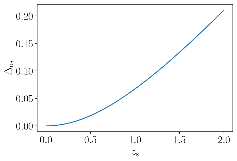
Figure 1: Evolution of the mean projected density term $\Delta_{\mathrm{os}}(z_{\mathrm{s}})$ defined in eq. 2.9 as a function of the redshift $z_{\mathrm{s}}$ of the source. We note that this quantity is non-negligible at high redshift, reaching about $10\text{\,}\mathrm{\char 37\relax}$ between $z=1$ and $1.5$.

The second quantity in eq. 2.8, $\bar{\kappa}_{\mathrm{os}}$, is a projection of the total density perturbation along the line of sight; it coincides with the weak-lensing convergence that would occur if matter were entirely diffuse, i.e., if the compact objects were smoothed out. For an overdense line of sight, $\bar{\kappa}_{\mathrm{os}}>0$, there are more compact objects and hence $\tau$ increases. We estimate the distribution of $\bar{\kappa}_{\mathrm{os}}$ from a combination of (i) publicly available numerical results from ray tracing in an $N$-body simulation [64] and (ii) standard cosmological calculations; see appendix A for details on the simulation and our fitting functions.

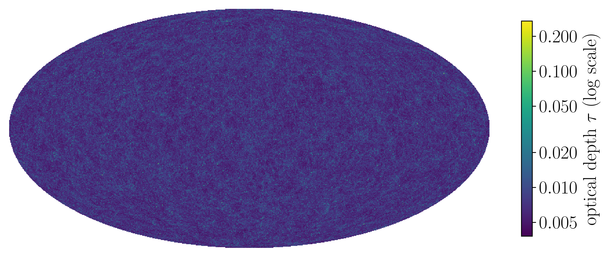
Figure 2: Simulated map of the microlensing optical depth $\tau$ (in logarithmic scale) in a universe with a fraction $\alpha=0.5$ of compact objects, and a source at $z_{\mathrm{s}}=0.45$. The sky is dominated by very low values of $\tau$, with rare occurrences of mild values.

For the sake of illustration, fig. 2 shows a sky map of the optical depth $\tau$ for $z_{\mathrm{s}}=0.45$ and a fraction $\alpha=0.5$ of compact objects. More quantitatively, our prediction for the PDF of the optical depth $\tau$ is shown in fig. 3 for various values of the fraction of compact objects $\alpha$ and of the source redshift $z_{\mathrm{s}}$. We can see that, except for sources located at high redshift and for a fraction of compact objects approaching unity, the optical depth remains at most on the percent order for most of the lines of sight.

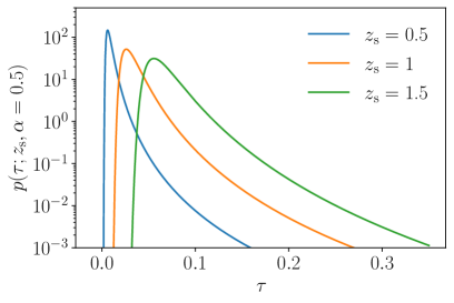
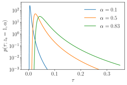
Figure 3: Probability density $p(\tau;z_{\mathrm{s}},\alpha)$ of the optical depth $\tau$ for a source at redshift $z_{\mathrm{s}}$ in a realistic universe made of a fraction $\alpha$ of compact objects. Left: effect the source redshift for $\alpha=0.5$. Right: effect of the fraction of compact objects for $z_{\mathrm{s}}=1$.

2.4 Relevant optical depths are not that low

The distributions shown in fig. 3 indicate that, except in rather extreme cases, most of the celestial sphere is characterised by a very low optical depth, thereby suggesting that the model of eq. 2.5 may be a good description of the amplification probabilities. However, this conclusion must be nuanced as we wish to focus on mild to high amplifications. Suppose for instance that we seek a microlensing signal in the Hubble diagram of type-Ia SNe, such as in refs. [34, 35, 37, 38]. To be detectable, the effect of microlensing should be larger than the intrinsic dispersion of SN magnitudes, $\sigma_{\mathrm{int}}\sim 0.1~{}\mathrm{mag}$ [65]. The decrease of an SN magnitude by $3\sigma_{\mathrm{int}}$ would be equivalent to an amplification factor $A=10^{6\sigma_{\mathrm{int}}/5}\approx 1.3$, which is considerable.

Although regions with large optical depth $\tau$ are rare, they are also expected to produce more detectable amplifications than the low-$\tau$ regions. The relevant question then becomes: are detectable amplifications mostly lying in low-$\tau$ regions, which cover most of the sky, or in the rarer but more efficient high-$\tau$ regions?

To answer this question, we adopt the following protocol. Let us focus on events with amplification $A>A_{1}=\sqrt{3}/5\approx 1.34$ corresponding to sources falling within the Einstein disk of a lens, and which coincidentally produce a $3\sigma$ effect on type-Ia SNe. In a region with optical depth $\tau$, this has a probability $P(A_{1};\tau)=1-\mathrm{e}^{-\tau}$ in the strongest-lens approach (2.5). So for the entire sky, the probability of such a high-amplification event would be

$$P(A_{1};z_{\mathrm{s}},\alpha)=\int_{0}^{\infty}\mathrm{d}\tau\;p(\tau;z_{\mathrm{s}},\alpha)\left(1-\mathrm{e}^{-\tau}\right),$$ (2.11)

for a fraction $\alpha$ of compact objects and a source at $z_{\mathrm{s}}$. Now suppose that we mask all the regions of the sky with an optical depth larger than $\tau_{\mathrm{m}}$; the probability would become

$$P_{\tau_{\mathrm{m}}}(A_{1};z_{\mathrm{s}},\alpha)=\frac{\int_{0}^{\tau_{\mathrm{m}}}\mathrm{d}\tau\;p(\tau;z_{\mathrm{s}},\alpha)\left(1-\mathrm{e}^{-\tau}\right)}{\int_{0}^{\tau_{\mathrm{m}}}\mathrm{d}\tau\;p(\tau;z_{\mathrm{s}},\alpha)}\ .$$ (2.12)

The ratio of those probabilities,

$$R(\tau_{\mathrm{m}},z_{\mathrm{s}},\alpha)\equiv\frac{P_{\tau_{\mathrm{m}}}(A_{1};z_{\mathrm{s}},\alpha)}{P(A_{1};z_{\mathrm{s}},\alpha)}\ ,$$ (2.13)

then defines the fraction of high-amplification events that survive the masking operation; in other words, $R(\tau_{\mathrm{m}})$ is the proportion of high-amplification events happening in regions whose optical depth is lower than $\tau_{\mathrm{m}}$.

The evolution of the ratio $R(\tau_{\mathrm{m}};z_{\mathrm{s}},\alpha)$ as a function of $\tau_{\mathrm{m}}$ is depicted in fig. 4 for various values of $z_{\mathrm{s}},\alpha$. For sources at high redshift, and for a non-negligible fraction of compact objects, we see that in order to properly account for, say, $99\text{\,}\mathrm{\char 37\relax}$ of the high-amplification events, we must allow the optical depth to reach values larger than $0.1$. Hence, as far as high amplifications ($A>1.34$) are concerned, the relevant regions of the sky do not necessarily have very low optical depths.

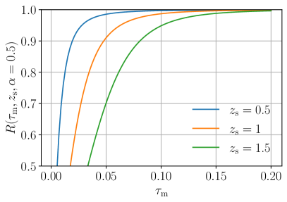
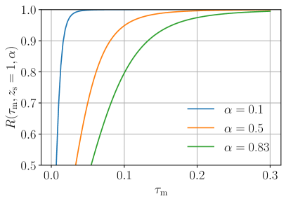
Figure 4: Proportion $R(\tau_{\mathrm{m}},z_{\mathrm{s}},\alpha)$ of the microlensing events with amplification $A>A_{1}\approx 1.34$ occurring within regions of the sky with optical depth lower than $\tau_{\mathrm{m}}$, for a source at $z_{\mathrm{s}}$ in a Universe with a fraction $\alpha$ of compact objects. Left: effect of the redshift of the source for $\alpha=0.5$. Right: effect of the fraction of compact objects for $z_{\mathrm{s}}=1$.

The general conclusion of the analysis conducted in this section is that we must a priori go beyond the simple model given by eqs. 2.5 and 2.6 in order to accurately model the statistics of extragalactic microlensing. This will be the purpose of the next two sections, where we propose a complete set of corrections to the strongest-lens approach.

3 Point lens with environment and line-of-sight perturbations

The discussion of sec. 2 suggests that the simplest modelling of extragalactic microlensing statistics – the strongest-lens approach sketched in subsec. 2.2 – may not be sufficient, because the relevant optical depths are low but not extremely low. In this context, we shall thus add perturbative corrections to this simple approach. We assume that when a source’s light is significantly amplified, lensing is still mostly due to a single lens, which we may call the dominant lens. However, we now allow for corrections due to the rest of the Universe – large-scale matter inhomogeneities, their substructure and the other compact lenses altogether – which we shall treat as tidal perturbations to the dominant lens.

In this section, we consider the problem of a single point lens that is perturbed by the presence of matter lumps in its environment and along the line of sight. We demonstrate that this problem can be suitably reformulated as a point lens with an external shear, and we derive the expression of the angular differential cross section $\Omega(A)$ of the amplification.

3.1 Description of the set-up

Figure 5: An extragalactic point-like source of light is observed through the inhomogeneous Universe. A fraction $\alpha$ of the matter density is made of compact objects, $\rho_{\mathrm{c}}(t,\bm{x})=\alpha\rho(t,\bm{x})$, while the rest is treated as diffuse matter. Since the microlensing optical depth associated with compact objects is small, any significant amplification is dominated by a single lens: the dominant lens.

The concrete situation that we consider is depicted in fig. 5. An extragalactic point-like source (supernova or quasar) at $z_{\mathrm{s}}$ is observed through an inhomogeneous universe. On large scales, we assume that the inhomogeneity of the matter distribution is well described by the $\Lambda$CDM cosmological model. On small scales, we assume that a fraction $\alpha$ of the total matter density is made of compact objects, which we model as point masses. Just like in subsec. 2.3, we assume that the distribution of compact objects closely follows the total matter density field: in a region with density $\rho(t,\bm{x})$, there is a Poisson-distributed population of compact objects with mean density $\rho_{\mathrm{c}}(t,\bm{x})\equiv\alpha\rho(t,\bm{x})$. We assume that $\alpha$ is constant in space and time.

Dominant lens

We define the dominant lens as the one that would produce the strongest amplification $A$ if it were alone in the Universe. Equivalently, it is the lens with the smallest reduced impact parameter $\beta/\theta_{\mathrm{E}}$, where $\beta$ is the angle between the unlensed source position and the lens position, and $\theta_{\mathrm{E}}$ its Einstein radius. We shall denote with a “d” subscript the quantities associated with the dominant lens, e.g., its redshift $z_{\mathrm{d}}$.

Tidal perturbations

All the other inhomogeneities of the Universe, which includes both astronomical structures and the non-dominant compact objects, are treated in the tidal regime. In the terminology of ref. [66], this means that apart from the immediate vicinity of the dominant lens, light propagates through a smooth space-time geometry. This is equivalent to stating that the angle between multiple images produced by the dominant lens, which is on the order of its Einstein radius $\theta_{\mathrm{E}}$, is much smaller than the typical scale over which the gravitational field produced by the other inhomogeneities changes appreciably. This notably requires all the non-dominant compact objects to lie far from the line of sight. In practice, the tidal approximation means that non-dominant inhomogeneities only produce weak-lensing convergence and shear which perturb the behaviour of the dominant lens.

3.2 Lens equation and equivalent lens

We now discuss the lens equation associated with the set-up described in subsec. 3.1. We then show that, with a suitable change of variables, it may be turned into the lens equation of a point lens with external shear.

3.2.1 Lens equation with tidal perturbations

Figure 6: Schematic representation of the quantities involved in the lens equation (3.1). The total displacement $\bm{\theta}-\bm{\beta}$ is caused by the dominant point-like lens and the tidal distortions $\bm{\mathcal{A}}_{\mathrm{od}},\bm{\mathcal{A}}_{\mathrm{ds}},\bm{\mathcal{A}}_{\mathrm{os}}$.

The relevant quantities defined below are depicted in fig. 6. The line of sight is conventionally set as the direction in which the main lens is observed. With respect to that origin, we call $\bm{\beta}$ the unlensed position of the source. Throughout this article, “unlensed” will refer to the case where light would propagate in the reference FLRW model. We denote with $\bm{\theta}$ the observed position of an image of the source.

The lens equation is the relation between $\bm{\theta}$ and $\bm{\beta}$. For a dominant point lens with tidal perturbation along the line of sight, it takes the form [67, 68, 69, 70, 71, 72, 66, 73]

$$\bm{\beta}=\bm{\mathcal{A}}_{\mathrm{os}}\,\bm{\theta}-\bm{\mathcal{A}}_{\mathrm{ds}}\,\bm{\alpha}_{\mathrm{PL}}(\bm{\mathcal{A}}_{\mathrm{od}}\bm{\theta})\ ,$$ (3.1)

where we have introduced some notation. The heart of eq. 3.1 is the displacement angle $\bm{\alpha}_{\mathrm{PL}}(\bm{\theta})$ of the dominant (point-like) lens only. In the absence of other inhomogeneities, we would simply have $\bm{\beta}=\bm{\theta}-\bm{\alpha}_{\mathrm{PL}}(\bm{\theta})$. Its explicit expression is

$$\bm{\alpha}_{\mathrm{PL}}(\bm{\theta})=\frac{\theta_{\mathrm{E}}^{2}\bm{\theta}}{|\bm{\theta}|^{2}}\equiv\frac{\theta_{\mathrm{E}}^{2}}{\bm{\theta}}\ ,$$ (3.2)

where $\theta_{\mathrm{E}}$ is the unperturbed angular Einstein radius,

$$\theta_{\mathrm{E}}^{2}\equiv\frac{4GmD_{\mathrm{ds}}}{D_{\mathrm{od}}D_{\mathrm{os}}}=\frac{4Gm(\chi_{\mathrm{s}}-\chi_{\mathrm{d}})}{a(\chi_{\mathrm{d}})\chi_{\mathrm{d}}\chi_{\mathrm{s}}}\ ,$$ (3.3)

and $m$ the mass of the dominant lens.

The three quantities $\bm{\mathcal{A}}_{\mathrm{od}},\bm{\mathcal{A}}_{\mathrm{os}},\bm{\mathcal{A}}_{\mathrm{ds}}$ are $2\times 2$ distortion matrices which encode the tidal perturbations along the line of sight. They are defined as follows: in the absence of the main lens, for an observer at (a) and source at (b), the unlensed position $\bm{\beta}_{\mathrm{ab}}$ and lensed position $\bm{\theta}_{\mathrm{ab}}$ of the source are related by $\bm{\beta}_{\mathrm{ab}}=\bm{\mathcal{A}}_{\mathrm{ab}}\bm{\theta}_{\mathrm{ab}}$. Thus, in the absence of the dominant lens [$\bm{\alpha}_{\mathrm{PL}}(\bm{\theta})=\bm{0}$] the lens equation would reduce to $\bm{\beta}=\bm{\mathcal{A}}_{\mathrm{os}}\bm{\theta}$, which corresponds to standard weak lensing [74]. The distortion matrices may be decomposed as

$$\bm{\mathcal{A}}_{\mathrm{ab}}=\bm{1}-\begin{bmatrix}\kappa_{\mathrm{ab}}+\mathrm{Re}(\gamma_{\mathrm{ab}})&\mathrm{Im}(\gamma_{\mathrm{ab}})-\omega_{\mathrm{ab}}\\ \mathrm{Im}(\gamma_{\mathrm{ab}})+\omega_{\mathrm{ab}}&\kappa_{\mathrm{ab}}-\mathrm{Re}(\gamma_{\mathrm{ab}})\end{bmatrix},\qquad\mathrm{a},\mathrm{b}\in\{\mathrm{o},\mathrm{d},\mathrm{s}\}\ .$$ (3.4)

In this decomposition, $\kappa_{\mathrm{ab}}\in\mathbb{R}$ represents the convergence that is be produced by the diffuse matter from (a) to (b); the symmetric trace-free part, encoded in $\gamma_{\mathrm{ab}}\in\mathbb{C}$, represents the shear produced in the same interval; the anti-symmetric part $\omega_{\mathrm{ab}}\in\mathbb{R}$ represents the solid rotation of images from (a) to (b).

In the following, we shall work at first order in the shear, $\gamma_{\mathrm{ab}}\ll 1$. In that regime, it can be shown that the rotation is a second-order quantity $\omega\sim|\gamma|^{2}$ (see ref. [75], sec. 2.3.2); we shall thus neglect $\omega_{\mathrm{ab}}$. However, as will be clearer in the very next paragraph, the convergence may reach values exceeding $10\text{\,}\mathrm{\char 37\relax}$, hence we shall work non-perturbatively in $\kappa_{\mathrm{ab}}$.

3.2.2 Physical origin of the convergence and shear

Let us now elaborate on the convergences $\kappa_{\mathrm{ab}}$ and shears $\gamma_{\mathrm{ab}}$ appearing in the distortion matrices that enter in the lens equation (3.1).

Convergence is due to the diffuse matter

that is intercepted by the line of sight. More precisely, $\kappa_{\mathrm{ab}}$ represents the excess (or deficit) of focusing from diffuse matter, with respect to the homogeneous FLRW reference, for a source located at (b) and observed from (a). Its explicit expression is

$$\kappa_{\mathrm{ab}} \equiv 4\pi G\int_{\chi_{\mathrm{a}}}^{\chi_{\mathrm{b}}}\mathrm{d}\chi\;\frac{(\chi-\chi_{\mathrm{a}})(\chi_{\mathrm{b}}-\chi)}{\chi_{\mathrm{b}}-\chi_{\mathrm{a}}}\,a^{2}(\chi)\left[(1-\alpha)\rho-\bar{\rho}\right]$$ (3.5)

$$=(1-\alpha)\bar{\kappa}_{\mathrm{ab}}-\alpha\Delta_{\mathrm{ab}}\ .$$ (3.6)

where $\Delta_{\mathrm{ab}}$ and $\bar{\kappa}_{\mathrm{ab}}$ are generalisations of the $\Delta_{\mathrm{os}}$ and $\bar{\kappa}_{\mathrm{os}}$ defined in eqs. 2.9 and 2.10,

$$\Delta_{\mathrm{ab}} \equiv 4\pi G\bar{\rho}_{0}\int_{\chi_{\mathrm{a}}}^{\chi_{\mathrm{b}}}\mathrm{d}\chi\;\frac{(\chi-\chi_{\mathrm{a}})(\chi_{\mathrm{b}}-\chi)}{\chi_{\mathrm{b}}-\chi_{\mathrm{a}}}\,\frac{1}{a(\chi)}\ ,$$ (3.7)

$$\bar{\kappa}_{\mathrm{ab}} \equiv 4\pi G\bar{\rho}_{0}\int_{\chi_{\mathrm{a}}}^{\chi_{\mathrm{b}}}\mathrm{d}\chi\;\frac{(\chi-\chi_{\mathrm{a}})(\chi_{\mathrm{b}}-\chi)}{\chi_{\mathrm{b}}-\chi_{\mathrm{a}}}\,\frac{\delta(\chi)}{a(\chi)}\ .$$ (3.8)

The first term in eq. 3.6 is quite intuitive; since the fraction of diffuse matter is $1-\alpha$, any excess $\bar{\kappa}_{\mathrm{ab}}$ in total projected density translates into $(1-\alpha)\bar{\kappa}_{\mathrm{ab}}$ from its diffuse component. The second term is more subtle; it encodes the deficit of diffuse matter, relative to FLRW, that occurs as one turns a fraction $\alpha$ of it into compact matter. In the extreme case $\alpha=1$, there is no diffuse matter at all, which implies a significant focusing deficit, $\kappa_{\mathrm{ab}}=-\Delta_{\mathrm{ab}}$, with respect to FLRW – this is Zel’dovich’s empty-beam case [63]. The presence of $\Delta_{\mathrm{ab}}$ in $\kappa_{\mathrm{ab}}$ is the reason why the convergence can reach relatively large values and should not be treated at linear order. Note finally that eqs. 2.8 and 3.6 imply the following relation between convergences and optical depth: $\kappa_{\mathrm{os}}=\bar{\kappa}_{\mathrm{os}}-\tau$.

Shear is due to both diffuse and compact matter

unlike convergence. This is because shear is associated with long-range tidal forces generated by any matter lump. For a source located at (b) and observed from (a), we may decompose the total shear as

$$\gamma_{\mathrm{ab}}=\bar{\gamma}_{\mathrm{ab}}+s_{\mathrm{ab}}\ .$$ (3.9)

In eq. 3.9, $\bar{\gamma}_{\mathrm{ab}}$ is the macroshear associated with the smooth density contrast, that is, the shear that would be produced on a beam of light in the absence of any compact object near the line of sight. Its formal expression is [76]

$$\bar{\gamma}_{\mathrm{ab}}=-4\pi G\bar{\rho}_{0}\int_{\chi_{\mathrm{a}}}^{\chi_{\mathrm{b}}}\mathrm{d}\chi\;\frac{(\chi-\chi_{\mathrm{a}})(\chi_{\mathrm{b}}-\chi)}{\chi_{\mathrm{b}}-\chi_{\mathrm{a}}}\int_{\mathbb{R}^{2}}\frac{\mathrm{d}^{2}\bm{r}}{\pi r^{2}}\;\frac{\delta(\chi,\bm{r})}{a(\chi)}\,\mathrm{e}^{2\mathrm{i}\varphi}\ ,$$ (3.10)

where $\bm{r}=r(\cos\varphi,\sin\varphi)$ denotes the physical transverse position of a point, orthogonally to the line of sight, $\mathrm{d}^{2}\bm{r}=r\mathrm{d}r\mathrm{d}\varphi$. Specifically, $r$ is the distance between a point and the line of sight and $\varphi$ is its polar angle about that axis.

The second term of eq. 3.9, $s_{\mathrm{ab}}$, is the microshear produced by compact objects in the vicinity of the line of sight, except the dominant lens. If the region between (a) and (b) contains $N$ point-like lenses labelled with $\ell$, then the microshear reads [73]

$$s_{\mathrm{ab}}=-4\pi G\sum_{\ell=1}^{N}\frac{(\chi_{\ell}-\chi_{\mathrm{a}})(\chi_{\mathrm{b}}-\chi_{\ell})}{\chi_{\mathrm{b}}-\chi_{\mathrm{a}}}\,\frac{a(\chi_{\ell})m_{\ell}}{\pi r_{\ell}^{2}}\,\mathrm{e}^{2\mathrm{i}\varphi_{\ell}}\ ,$$ (3.11)

where $m_{\ell}$ is the mass of lens $\ell$, $\chi_{\ell}$ its comoving distance from the observer, $r_{\ell}$ its physical distance from the optical axis and $\varphi_{\ell}$ its polar angle about it. Note that eq. 3.10 is nothing but the continuous limit of eq. 3.11.

The careful reader may have noticed that the macroshear $\bar{\gamma}_{\mathrm{ab}}$ does not come with any prefactor $(1-\alpha)$. Such a prefactor could be expected indeed, to avoid double-counting the shear of compact matter, which should be encoded in $s_{\mathrm{ab}}$ already. The reason is that, in the following, we shall compute $s_{\mathrm{ab}}$ as if the compact objects were randomly distributed transversely to the line of sight. Hence, $s_{\mathrm{ab}}$ will not account for the large-scale clustering of those objects. Because they follow the total matter density contrast $\delta(t,\bm{x})$ on large scales, their contribution to cosmic shear is essentially the same as if they were replaced by diffuse matter. Therefore, $\bar{\gamma}_{\mathrm{ab}}$ is unchanged under changes of the compact matter fraction $\alpha$. Increasing $\alpha$ only produces more shear via $s_{\mathrm{ab}}$.

3.2.3 Equivalent lens

The lens equation (3.1) contains a priori nine real parameters besides the dominant lens’s Einstein radius: the three convergences and the six shear components. But only a few specific combinations of those parameters turn out to be relevant to the problem of amplification probabilities. Multiplying eq. 3.1 to the left with $(1-\kappa_{\mathrm{od}})(1-\kappa_{\mathrm{os}})^{-1}(1-\kappa_{\mathrm{ds}})\bm{\mathcal{A}}_{\mathrm{ds}}^{-1}$ and working at first order in the shears, we find the equivalent lens equation

$$\tilde{\bm{\beta}}=(1-\bm{\Gamma})\,\tilde{\bm{\theta}}-\frac{\tilde{\theta}_{\mathrm{E}}^{2}}{\tilde{\bm{\theta}}}\ ,$$ (3.12)

whose new variables are

$$\tilde{\bm{\beta}} \equiv\frac{(1-\kappa_{\mathrm{od}})(1-\kappa_{\mathrm{ds}})}{1-\kappa_{\mathrm{os}}}\,\bm{\mathcal{A}}_{\mathrm{ds}}^{-1}\bm{\beta}\ ,$$ (3.13)

$$\tilde{\bm{\theta}} \equiv\bm{\mathcal{A}}_{\mathrm{od}}\bm{\theta}\ ,$$ (3.14)

and the new parameters read

$$\tilde{\theta}_{\mathrm{E}} \equiv\sqrt{\frac{(1-\kappa_{\mathrm{od}})(1-\kappa_{\mathrm{ds}})}{1-\kappa_{\mathrm{os}}}}\,\theta_{\mathrm{E}}\ ,$$ (3.15)

$$\bm{\Gamma} \equiv\begin{bmatrix}\mathrm{Re}(\gamma)&\mathrm{Im}(\gamma)\\ \mathrm{Im}(\gamma)&-\mathrm{Re}(\gamma)\end{bmatrix},\qquad\gamma\equiv\frac{\gamma_{\mathrm{os}}}{1-\kappa_{\mathrm{os}}}-\frac{\gamma_{\mathrm{od}}}{1-\kappa_{\mathrm{od}}}-\frac{\gamma_{\mathrm{ds}}}{1-\kappa_{\mathrm{ds}}}\ .$$ (3.16)

In other words, under the linear change of variables $(\bm{\beta},\bm{\theta})\mapsto(\tilde{\bm{\beta}},\tilde{\bm{\theta}})$, our initial problem of a point lens with generic tidal perturbations has turned into the much simpler eq. 3.12, which describes a point mass with an external shear $\gamma$ in the same plane. This equivalent problem has been well studied since the 1980s [46, 49, 77].

3.3 Amplification cross section

Let us use the equivalent lens model (3.12) to derive the amplification cross section. We define the differential amplification cross section $\Omega(A)$ so that $\Omega(A)\mathrm{d}A$ is the angular area (solid angle) of the region of the sky where the amplification is between $A$ and $A+\mathrm{d}A$.

3.3.1 For the equivalent lens

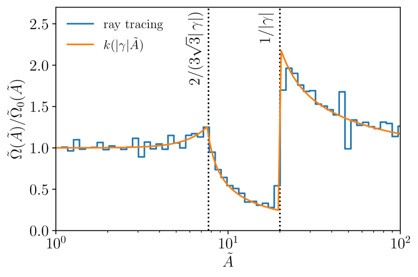
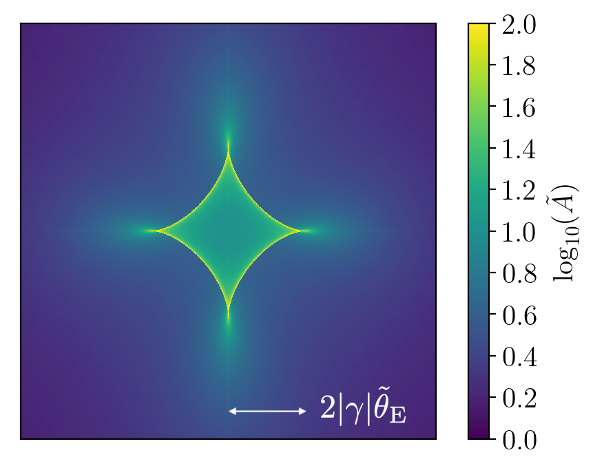
Figure 7: Properties of the equivalent point lens with external shear. Left panel: Ratio of the amplification cross section $\tilde{\Omega}(\tilde{A})$ in the presence of shear (here $\gamma=0.05$) with the no-shear case $\tilde{\Omega}_{0}(\tilde{A})$ (3.17). The solid-line histogram shows results from ray tracing, while the dashed line shows the analytical fit $k(|\gamma|\tilde{A})$ of eq. 3.19 as proposed in ref. [77]. Right panel: Amplification map $\tilde{A}(\tilde{\bm{\beta}})$. The astroid-shaped caustic has a size $2|\gamma|\tilde{\theta}_{\mathrm{E}}$; inside the astroid a source has four images, outside it has two images, and exactly on it it has three images among which one is infinitely amplified.

We first work in the twiddled world described by eq. 3.12. If the effective shear $\gamma$ were zero, then the problem would reduce to a single point lens whose constant-amplification contours are circles, with radius $\tilde{\beta}_{0}(\tilde{A})=\tilde{\theta}_{\mathrm{E}}\,[2\tilde{A}/(\tilde{A}^{2}-1)^{1/2}-2]^{1/2}$. The cross section would thus read, in this simple case,

$$\tilde{\Omega}_{0}(\tilde{A})=2\pi\tilde{\beta}_{0}(\tilde{A})\left|\frac{\mathrm{d}\tilde{\beta}_{0}}{\mathrm{d}{\tilde{A}}}\right|=\frac{2\pi\tilde{\theta}_{\mathrm{E}}^{2}}{(\tilde{A}^{2}-1)^{3/2}}\ .$$ (3.17)

The problem is more involved in the presence of shear. In that case the source plane displays two distinct regions separated by an astroid-shaped caustic (see right panel of fig. 7). Outside the caustic a source has two images while inside it has four images. The shear $\gamma$ fixes the size and orientation of the astroid. To the best of our knowledge there is no analytic expression for the amplification $\tilde{A}(\tilde{\bm{\beta}})$ or its contours in that case. Nevertheless, Nityanda & Ostriker [46] noticed the remarkable fact that for low values of the shear $|\gamma|$, corrections the the amplification cross section should only depend on the product $|\gamma|A$. More than a decade later, Kofman et al. [77] further pushed this idea by writing

$$\tilde{\Omega}(\tilde{A})=\tilde{\Omega}_{0}(\tilde{A})\,k(|\gamma|\tilde{A})\ ,$$ (3.18)

where $\tilde{\Omega}_{0}(\tilde{A})$ is the no-shear cross section of eq. 3.17, while $k$ is a function fitted from numerical simulations,

$$k(x)=\begin{cases}1+7.7\,x^{3.5}&\displaystyle x\leq\frac{2}{3\sqrt{3}}\ ,\\[11.38109pt] \displaystyle\frac{0.17}{(x-0.33)^{1/2}}+\frac{0.023}{x-0.33}&\displaystyle\frac{2}{3\sqrt{3}}\leq x\leq 1\ ,\\[11.38109pt] \displaystyle 1+\frac{0.85}{x}+\frac{0.37}{x^{5}}&\displaystyle x\geq 1\ .\end{cases}$$ (3.19)

For the sake of completeness, we have reproduced in fig. 7 the comparison between numerical ray tracing and Kofman et al.’s result (3.18) for $\gamma=0.05$. The simulation uses inverse ray tracing with a simple adaptive mesh refinement, see ref. [57] for details. Agreement is excellent.

3.3.2 Back to the original problem

We now translate the results of the twiddled world in terms of $\Omega(A)$. The first step is to express $\tilde{A}$ in terms of $A$. At first order in the shear, we find

$$\tilde{A}\equiv\frac{\mathrm{d}^{2}\tilde{\bm{\theta}}}{\mathrm{d}^{2}\tilde{\bm{\beta}}}=\frac{(1-\kappa_{\mathrm{os}})^{2}}{(1-\kappa_{\mathrm{od}})^{2}(1-\kappa_{\mathrm{ds}})^{2}}\,\frac{\det\bm{\mathcal{A}}_{\mathrm{od}}}{\det\bm{\mathcal{A}}_{\mathrm{ds}}^{-1}}\,\frac{\mathrm{d}^{2}\bm{\theta}}{\mathrm{d}^{2}\bm{\beta}}=(1-\kappa_{\mathrm{os}})^{2}A\ .$$ (3.20)

The conversion of $\tilde{\Omega}$ into $\Omega$ must take two aspects into account. On the one hand, since those are differential cross sections, their relation involves the Jacobian $|\mathrm{d}\tilde{A}/\mathrm{d}A|$, just like when one changes variables in a probability density function, for example. Second, since $\tilde{\Omega}$ is a cross section in the twiddled source plane, it is expressed in the twiddled units $[\tilde{\beta}]^{2}$, which differ from the units $[\beta]^{2}$ of the original source plane. Taking both aspects into account yields

$$\Omega(A)\,\mathrm{d}A=\frac{\mathrm{d}^{2}\bm{\beta}}{\mathrm{d}^{2}\tilde{\bm{\beta}}}\times\tilde{\Omega}(\tilde{A})\,\mathrm{d}\tilde{A}\ .$$ (3.21)

Substituting eqs. 3.13, 3.20 and 3.18 into eq. 3.21, and still working at first order in the shear, we find the following elegant expression for the cross section,

$$\Omega(A)=2\pi\vartheta_{\mathrm{E}}^{2}\,k\left(\frac{|\gamma|A}{A_{\mathrm{min}}}\right)\,\frac{A_{\mathrm{min}}^{2}}{(A^{2}-A_{\mathrm{min}}^{2})^{3/2}}\ ,$$ (3.22)

where $A_{\mathrm{min}}\equiv(1-\kappa_{\mathrm{os}})^{-2}$ is the minimal amplification in this setup, i.e. the amplification that would be observed if the dominant lens were infinitely far from the line of sight, so that only the weak-lensing convergence is at play. It is implicit that $\Omega(A<A_{\mathrm{min}})=0$. Besides, we have introduced $\vartheta_{\mathrm{E}}$ such that

$$\vartheta_{\mathrm{E}}^{2}\equiv\frac{(1-\kappa_{\mathrm{ds}})\,\theta_{\mathrm{E}}^{2}}{(1-\kappa_{\mathrm{od}})(1-\kappa_{\mathrm{os}})}=\frac{4Gm(1-\kappa_{\mathrm{ds}})D_{\mathrm{ds}}}{(1-\kappa_{\mathrm{od}})D_{\mathrm{od}}(1-\kappa_{\mathrm{os}})D_{\mathrm{os}}}\ .$$ (3.23)

Physically, $\vartheta_{\mathrm{E}}$ represents the the lensed Einstein radius, i.e. the size of the Einstein ring that would be observed if the source were perfectly aligned with the dominant lens in the presence of the external convergences; this can be checked by setting $\bm{\beta}=\bm{0}$ in eq. 3.1.

Summarising, the convergence due to diffuse matter has two distinct effect on $\Omega(A)$: (i) they rescale amplifications according to $A\to A/A_{\mathrm{min}}=(1-\kappa_{\mathrm{os}})^{2}A$, thereby fixing the minimum amplification accessible to the system; (ii) they rescale the dominant lens’s Einstein radius as $\theta_{\mathrm{E}}\to\vartheta_{\mathrm{E}}$, thereby changing the cross section directly. The shear, due to both diffuse and compact matter, affects $\Omega(A)$ via Kofman et al.’s function $k(|\gamma|A/A_{\mathrm{min}})$ only.

4 Amplification probabilities

In the previous section, we have derived the amplification cross section $\Omega(A)$ for a single point lens with perturbations (3.22). We shall now turn this result into a PDF for the amplification, $p(A)$, using the statistical properties of the dominant lens and its perturbations.

4.1 Amplification probability for a single lens

In realistic scenarios where the mass of the compact objects is small (e.g. comparable to a solar mass), then the typical angle separating two such objects is much smaller than the angular scales over which $\bar{\kappa},\bar{\gamma},\tau$ are changing appreciably. Thus, we may consider a “mesoscopic” cone with half angle $\Theta$ at the observer which contains a large number of compact objects, but across which the macroscopic quantities $\bar{\kappa},\bar{\gamma},\tau$ are constant (see fig. 8). Since those empirically show significant changes on the arcmin scale, we have $\Theta\ll 1$.

Figure 8: Mesoscopic cone with half angle $\Theta$ at the observer, containing a large number of compact objects, but across which the macroscopic quantities $\tau,\bar{\kappa},\bar{\gamma}$ can be considered constant.

The first step of our calculation consists in expressing the PDF $p_{1}(A)$ of the amplification due to one dominant lens in the mesoscopic cone. If all the parameters entering the amplification cross section (3.22) were fixed, then we would have by definition $p_{1}(A)=\Omega(A)/(\pi\Theta^{2})$. But since the properties of the main lens – namely its mass $m$ and comoving distance $\chi$ from the observer – and the microshear $s=\gamma-\bar{\gamma}$ vary a lot across the mesoscopic cone, we must marginalise over their statistical distribution,

$$p_{1}(A)=\frac{1}{\pi\Theta^{2}}\int\mathrm{d}m\,\mathrm{d}\chi\,\mathrm{d}^{2}s\;p(m,\chi,s)\,\Omega(A;m,\chi,|\bar{\gamma}+s|)\ ,$$ (4.1)

where $\Omega$ depends on $m$ via the Einstein radius of the dominant lens, $\theta_{\mathrm{E}}^{2}\propto m$, and on $\chi$ via $\theta_{\mathrm{E}}$ and the (od), (ds) convergences and shears. We did not explicitly include the fixed macroscopic parameters $\tau,\bar{\kappa}_{\mathrm{os}},\bar{\gamma}_{\mathrm{os}}$ to alleviate notation.

4.1.1 Approximations

In order to model the joint distribution $p(m,\chi,s)$, we make the following assumptions:

1. The mass $m$ of the dominant lens is uncorrelated with the other parameters. Since $\Omega\propto m$, this implies that we may simply replace $m$ by its average value $\left\langle m\right\rangle$ in the remainder of this calculation.

2. Compact objects are randomly distributed in space and their comoving number density $n_{\mathrm{c}}$ is constant within the mesoscopic cone. This implies, in particular, that $p(\chi)=3\chi^{2}/\chi_{\mathrm{s}}^{3}$.

Besides, in order to simplify the evaluation of the various convergences and shears involved in $\Omega(A)$, we shall adopt the following mean-field approximation:

$$\bar{\kappa}_{\mathrm{ab}}\approx\left(\frac{\chi_{\mathrm{b}}-\chi_{\mathrm{a}}}{\chi_{\mathrm{s}}}\right)^{2}\bar{\kappa}_{\mathrm{os}}\ ,\qquad\bar{\gamma}_{\mathrm{ab}}\approx\left(\frac{\chi_{\mathrm{b}}-\chi_{\mathrm{a}}}{\chi_{\mathrm{s}}}\right)^{2}\bar{\gamma}_{\mathrm{os}}\ .$$ (4.2)

The intuition behind this approximation appears by examining the integrals (3.8) and (3.10) defining $\bar{\kappa}_{\mathrm{ab}}$ and $\bar{\gamma}_{\mathrm{ab}}$. Consider all the possible lines of sight with the same fixed $\bar{\kappa}_{\mathrm{os}}$, $\bar{\gamma}_{\mathrm{os}}$. They are in principle quite diverse, because the matter density contrast $\delta$ may display significant variations along them, and hence they may have a variety of $\bar{\kappa}_{\mathrm{od}},\bar{\kappa}_{\mathrm{ds}},\bar{\gamma}_{\mathrm{od}},\bar{\gamma}_{\mathrm{ds}}$. However, on average all the elements $\mathrm{d}\chi$ along the line of sight should conspire so as to produce the required $\bar{\kappa}_{\mathrm{os}},\bar{\gamma}_{\mathrm{os}}$. If we neglect the effect of dark energy on structure formation, we know that $\delta\propto a$, which motivates us to consider that the mean-field contribution of $\delta(\chi)/a(\chi)$ to $\bar{\kappa}_{\mathrm{ab}},\bar{\gamma}_{\mathrm{ab}}$ is independent of $\chi$. As the latter is taken off the integrals over $\chi$, eqs. 3.8 and 3.10 imply

$$\bar{\kappa}_{\mathrm{ab}},\bar{\gamma}_{\mathrm{ab}}\propto\int_{\chi_{\mathrm{a}}}^{\chi_{\mathrm{b}}}\mathrm{d}\chi\;\frac{(\chi-\chi_{\mathrm{a}})(\chi_{\mathrm{b}}-\chi)}{\chi_{\mathrm{b}}-\chi_{\mathrm{a}}}\propto(\chi_{\mathrm{b}}-\chi_{\mathrm{a}})^{2}\ ,$$ (4.3)

whence eq. 4.2. We shall also apply a similar rule to the full convergence $\kappa_{\mathrm{ab}}$.

The difficult step then consists in determining the distribution for the microshear, and evaluating its consequences on $p_{1}(A)$.

4.1.2 Distribution of the microshear

The statistics of the shear caused by a random distribution of point masses has been, in fact, a well-know problem for a long time. It was first considered for masses placed in the same plane by Nityananda & Ostriker [46], using one of the methods exposed in the famous review [78] by Chandrasekhar in 1943 on statistical problems in astrophysics. However, the very last step of the calculation was only performed three years later by Schneider [79]. The result was then generalised to any lens profile by Lee & Spergel [50] and finally to multiple lens planes in Lee et al. [51].

In the case that we are interested in here, if the dominant lens is fixed at a comoving distance $\chi$ from the observer, then the reduced microshear $s=s_{\mathrm{os}}/(1-\kappa_{\mathrm{os}})-s_{\mathrm{od}}/(1-\kappa_{\mathrm{od}})-s_{\mathrm{ds}}/(1-\kappa_{\mathrm{ds}})$ caused by the other compact objects has an amplitude $S\equiv|s|$ distributed as

$$p(S;\chi)\,\mathrm{d}S=\frac{f(\chi)\tau S\,\mathrm{d}S}{[f^{2}(\chi)\tau^{2}+S^{2}]^{3/2}}\ ,\qquad P(S;\chi)=\left[1-\frac{S^{2}}{f^{2}(\chi)\tau^{2}}\right]^{-1/2}\ .$$ (4.4)

Equation 4.4 is controlled by an effective optical depth $f\tau$, with

$$f(\chi;\chi_{\mathrm{s}},\kappa_{\mathrm{os}}) \equiv\frac{\int_{0}^{\chi}\frac{\mathrm{d}\chi^{\prime}}{a(\chi^{\prime})}\left[\frac{\chi^{\prime}(\chi_{\mathrm{s}}-\chi^{\prime})}{(1-\kappa_{\mathrm{os}})\chi_{\mathrm{s}}}-\frac{\chi^{\prime}(\chi-\chi^{\prime})}{[1-\kappa_{\mathrm{od}}(\chi)]\chi}\right]+\int_{\chi}^{\chi_{\mathrm{s}}}\frac{\mathrm{d}\chi^{\prime}}{a(\chi^{\prime})}\left[\frac{\chi^{\prime}(\chi_{\mathrm{s}}-\chi^{\prime})}{(1-\kappa_{\mathrm{os}})\chi_{\mathrm{s}}}-\frac{(\chi^{\prime}-\chi)(\chi_{\mathrm{s}}-\chi^{\prime})}{[1-\kappa_{\mathrm{ds}}(\chi)](\chi_{\mathrm{s}}-\chi)}\right]}{\int_{0}^{\chi_{\mathrm{s}}}\frac{\mathrm{d}\chi^{\prime}}{a(\chi^{\prime})}\;\frac{\chi^{\prime}(\chi_{\mathrm{s}}-\chi^{\prime})}{\chi_{\mathrm{s}}}}$$ (4.5)

$$\approx\frac{1}{(1-\kappa_{\mathrm{os}})^{7/4}}\,\frac{2\chi}{\chi_{\mathrm{s}}}\left(1-\frac{\chi}{\chi_{\mathrm{s}}}\right).$$ (4.6)

The last approximation holds when the scale factor can be considered constant in the integrals (i.e. for $\chi_{\mathrm{s}}\to 0$) and in the mean-field approximation for $\kappa_{\mathrm{od}},\kappa_{\mathrm{ds}}$. The $(1-\kappa_{\mathrm{os}})^{-7/4}$ is empirical. The shape of the function $f(\chi)$ for various values of the source redshift and external convergence $\kappa_{\mathrm{os}}$ is depicted in fig. 9. Since the derivation of eq. 4.4 in ref. [51] uses different conventions and notation, we propose a full derivation in appendix B for completeness.

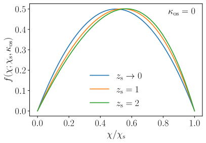
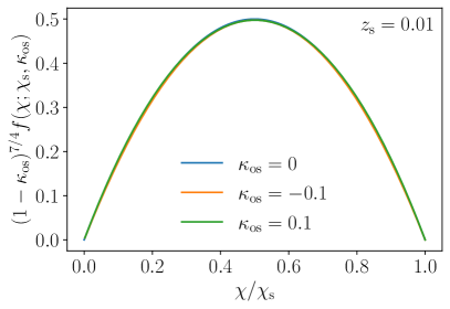
Figure 9: Factor $f(\chi;\chi_{\mathrm{s}},\kappa_{\mathrm{s}})$ defined in eq. 4.5 as a function of the ratio $\chi/\chi_{\mathrm{s}}$. Left: showing the dependence on the source redshift, by comparing $z_{\mathrm{s}}\to 0$ to $z_{\mathrm{s}}=1,2$ for $\kappa_{\mathrm{os}}=\kappa_{\mathrm{od}}=\kappa_{\mathrm{ds}}=0$. Right: showing the dependence in $\kappa_{\mathrm{os}}$ in the mean-field approximation, for $z_{\mathrm{s}}\ll 1$.

Let us finally point out that eq. 4.4 is actually an approximation where high values of $S$ are overestimated. Indeed, the compact objects responsible for the microshear are, by definition, non-dominant lenses. As such, their individual shear should not exceed the one that would be produced by the dominant lens if it were alone. So in principle $p(S)$ should also depend on, e.g., the impact parameter of the dominant lens $\beta_{\mathrm{d}}$, which would set an upper bound on $S$. This upper bound would go to infinity as $\beta_{\mathrm{d}}\rightarrow 0$, i.e. for large values of the amplification. Albeit more rigorous, these considerations would significantly complicate the treatment of the problem. We thus choose to ignore them, with the perspective of placing an upper bound on the effect of the microshear on $p(A)$.

4.1.3 The macroshear is negligible

The total shear $\gamma=\bar{\gamma}+s$ is the sum of the microshear $s$ discussed above with the macroshear $\bar{\gamma}$ due to the large-scale structure. While the distribution of microshear has a heavy tail, $\mathrm{Prob}(>S)\propto S^{-1}$, it turns out that the macroshear does not share this property, because the structures producing it are more diffuse. As shown in subsec. A.2, the conditional PDF of the macroshear at fixed convergence is surprisingly well fit by a two-dimensional Gaussian distribution, which therefore predicts very few high values for the macroshear.

Note that $s$ must be compared with $\bar{\gamma}\equiv\bar{\gamma}_{\mathrm{os}}/(1-\kappa_{\mathrm{os}})-\bar{\gamma}_{\mathrm{od}}/(1-\kappa_{\mathrm{od}})-\bar{\gamma}_{\mathrm{ds}}/(1-\kappa_{\mathrm{ds}})$ rather than with $\bar{\gamma}_{\mathrm{os}}$ alone. The difficulty is that ray tracing in numerical simulations is performed for a unique observer at present time; they allow one to compute $\bar{\gamma}_{\mathrm{os}},\bar{\gamma}_{\mathrm{od}}$, but not $\bar{\gamma}_{\mathrm{ds}}$. To circumvent this issue we apply again the mean-field approximation introduced in subsubsec. 4.1.1, which yields

$$\bar{\gamma}\approx f\,\bar{\gamma}_{\mathrm{os}}\ ,$$ (4.7)

with $f$ defined in eq. 4.5. It is not surprising to find here the same correction factor $f$ as for the effective optical depth of microshear: both have the same origin. Within that approximation, the PDF of $|\bar{\gamma}|$ is obtained from eq. A.10 by simple rescaling.

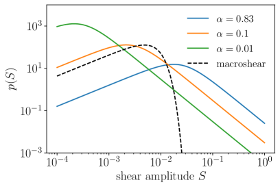
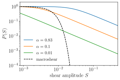
Figure 10: Distributions of the amplitude of microshear (solid lines), if the source located at $z_{\mathrm{s}}=0.95$ and the dominant lens at $z=0.5$. The left panel shows PDFs while the right panel shows CDFs. Three values for the fraction of compact matter are considered, $\alpha=0.83,0.1,0.01$. Dashed lines indicate the distributions of the amplitude of the macroshear $|\bar{\gamma}|\approx f|\gamma_{\mathrm{os}}|$, for lines of sight with $\bar{\kappa}_{\mathrm{os}}=0$.

Figure 10 compares the distributions of the microshear and macroshear amplitudes, for a source at $z_{\mathrm{s}}=0.95$, a dominant lens at $z=0.5$, and for a line of sight with $\bar{\kappa}_{\mathrm{os}}=0$ for simplicity. Three values for the fraction of compact matter are considered, $\alpha=0.83,0.1,0.01$ – the first case would correspond to the whole DM being made of compact objects. Those values correspond, respectively, to the effective optical depths $f\tau=2.5\times 10^{-2},3.0\times 10^{-3},3.0\times 10^{-4}$. Although the macroshear is generally not negligible compared to the microshear, especially when $\alpha$ is small, it is unable to produce large amplitudes. But large values of the shear are necessary to produce changes in $\Omega(A)$ at reasonable amplifications, $A<10$ (see subsec. 3.3). In the situation illustrated here, $|\bar{\gamma}|<$3\text{\,}\mathrm{\char 37\relax}$$ which would only affect $\Omega(A\gtrsim 13)$. Summarising, when macroshear is comparable to, or even larger than, microshear, then both have a negligible impact on the amplification statistics anyway. We shall thus neglect macroshear from now on, and replace $\Omega(A;m,\chi,|\bar{\gamma}+s|)$ with $\Omega(A;m,\chi,S)$ in eq. 4.1.

4.1.4 Final expression of $p_{1}(A)$

Substituting, in eq. 4.1, the probability density $p(m,s,\chi)=p(m)\,p(S;\chi)\,p(\chi)$ – where $p(S;\chi)$ is given by eq. 4.4 – and the expression (3.22) of $\Omega(A;m,\chi,S)$, and performing the change of variable $S\mapsto y\equiv S/f\tau$, we find

$$p_{1}(A)=\frac{2}{\Theta^{2}}\,\frac{A_{\mathrm{min}}^{2}}{(A^{2}-A_{\mathrm{min}}^{2})^{3/2}}\int_{0}^{\chi_{\mathrm{s}}}\mathrm{d}\chi\;p(\chi)\big{\langle}\vartheta_{\mathrm{E}}^{2}(\chi)\big{\rangle}_{m}K\left[\frac{f(\chi)\tau A}{A_{\mathrm{min}}}\right]\ ,$$ (4.8)

where $\left\langle\ldots\right\rangle_{m}$ denotes an average over the mass $m$ of the dominant lens, and

$$K(x)\equiv\int_{0}^{\infty}\mathrm{d}y\;\frac{y\,k(xy)}{(1+y^{2})^{3/2}}\approx 1-0.81\,x^{2}(1-3x)\left(1+\frac{3}{2}\,x^{3/2}\right)^{-8/3}\ .$$ (4.9)

The last step of the simplification of $p_{1}(A)$ consists in fully isolating the effect of the (micro)shear. For that purpose, we may multiply and divide eq. 4.8 with the average value of the weakly lensed squared Einstein radius,

$$\big{\langle}\vartheta_{\mathrm{E}}^{2}\big{\rangle}\equiv\int_{0}^{\chi_{\mathrm{s}}}\mathrm{d}\chi\;p(\chi)\big{\langle}\vartheta_{\mathrm{E}}^{2}(\chi)\big{\rangle}_{m}=\frac{4G\left\langle m\right\rangle}{(1-\kappa_{\mathrm{os}})\chi_{\mathrm{s}}}\int_{0}^{\chi_{\mathrm{s}}}\frac{\mathrm{d}\chi}{a(\chi)}\;\frac{1-\kappa_{\mathrm{ds}}(\chi)}{1-\kappa_{\mathrm{od}}(\chi)}\,\chi(\chi_{\mathrm{s}}-\chi)\ ,$$ (4.10)

to get

$$p_{1}(A)=\frac{2\left\langle\vartheta_{\mathrm{E}}^{2}\right\rangle}{\Theta^{2}}\,\frac{A_{\mathrm{min}}^{2}}{(A^{2}-A_{\mathrm{min}}^{2})^{3/2}}\,\mathcal{K}\left[\frac{\tau}{(1-\kappa_{\mathrm{os}})^{7/4}}\frac{A}{A_{\mathrm{min}}}\right]\ ,$$ (4.11)

with the last function that we shall define in this derivation:

$$\mathcal{K}(x)\equiv\frac{\int_{0}^{\chi_{\mathrm{s}}}\frac{\mathrm{d}\chi}{a(\chi)}\;\frac{1-\kappa_{\mathrm{ds}}(\chi)}{1-\kappa_{\mathrm{od}}(\chi)}\,\chi(\chi_{\mathrm{s}}-\chi)\,K[(1-\kappa_{\mathrm{os}})^{7/4}f(\chi)x]}{\int_{0}^{\chi_{\mathrm{s}}}\frac{\mathrm{d}\chi}{a(\chi)}\;\frac{1-\kappa_{\mathrm{ds}}(\chi)}{1-\kappa_{\mathrm{od}}(\chi)}\,\chi(\chi_{\mathrm{s}}-\chi)\,}\ .$$ (4.12)

The presence of the $(1-\kappa_{\mathrm{os}})^{7/4}$ factor in the argument of $K$ in eq. 4.12 is designed to absorb the empirical dependence on $\kappa_{\mathrm{os}}$ in $f$, and hence make $\mathcal{K}(x)$ practically insensitive to $\kappa_{\mathrm{os}}$.

The function $\mathcal{K}(x)$ defined in eq. 4.12 fully encapsulates the effect of the microshear. In principle, this function depends on the source redshift $z_{\mathrm{s}}$ via $\chi_{\mathrm{s}}=\chi(z_{\mathrm{s}})$, and on the macrostructure along the line of sight via $\kappa_{\mathrm{os}},\kappa_{\mathrm{od}},\kappa_{\mathrm{ds}}$. In practice, however, fig. 11 shows that $\mathcal{K}(x)$ is quite insensitive to those parameters. Such an empirical independence of $\mathcal{K}(x)$ in its external parameters encourages us to look for a simple and universal fitting function for it. We find that

$$\mathcal{K}(x)=1-0.254\,x^{2.33}\left(1-1.30\,x\right)\left[1+\frac{5}{4}\left(\frac{x}{1.83}\right)^{5/4}\right]^{-3.43}$$ (4.13)

provides an excellent fit, with an accuracy of a few parts in $10^{4}$ (see fig. 11).

The main conclusion of this subsection is that, to an excellent level of precision, the effect of the microshear on $p_{1}(A)$ mostly depends on the optical depth $\tau$. It reduces by about $1\text{\,}\mathrm{\char 37\relax}$ the probability of amplifications $A\sim 1/\tau$, and enhances larger ones ($A\sim 10/\tau$) by about $15\text{\,}\mathrm{\char 37\relax}$. Since we are considering low values for the optical depths, we can already anticipate that the net impact of shear on reasonable amplifications will be negligible.

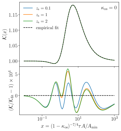
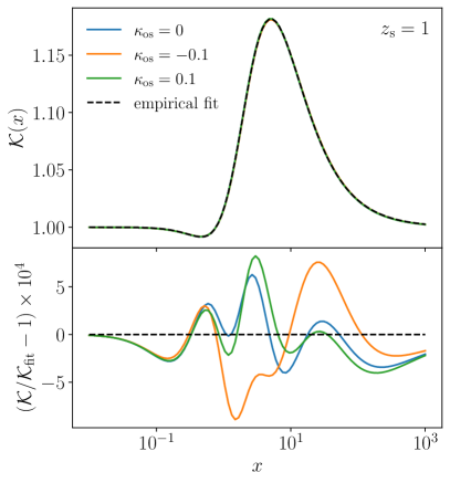
Figure 11: Integral $\mathcal{K}(x)$ defined in LABEL:{eq:integral_cal_K_definition} as a function of $x=(1-\kappa_{\mathrm{os}})^{-7/4}\tau A/A_{\mathrm{min}}$, which encapsulates all the microshear corrections to $p_{1}(A)$, with the empirical fitting function proposed in eq. 4.13. Left: Checking the dependence in $\chi_{\mathrm{s}}=\chi(z_{\mathrm{s}})$, for a fixed $\kappa_{\mathrm{os}}=0$. Right: Checking the dependence in $\kappa_{\mathrm{os}}$ for $z_{\mathrm{os}}=1$. The bottom panels show the relative accuracy of the empirical fit. We can see that $\mathcal{K}$ is mostly insensitive to both $z_{\mathrm{s}}$ and $\kappa_{\mathrm{os}}$, and that the fitting function is an excellent approximation.

4.2 From one lens to many: the strongest-perturbed-lens prescription

Now that we dispose of an accurate expression for the amplification PDF $p_{1}(A)$ of a single perturbed lens within a mesoscopic cone (fig. 8), we can generalise it to a large number $N\gg 1$ of such lenses. For that purpose, we shall adapt the strongest-lens prescription of subsec. 2.2, which consists in assuming that the total amplification $A$ produced by the $N$ perturbed lenses in the cone, is well-approximated by the amplification due to the strongest of them. Importantly, that is not to say that we are entirely neglecting the effect of the other lenses, because it is already encoded in the convergence and microshear corrections. As such, the strongest-perturbed-lens approach must be understood as a statistical prescription that is physically consistent with the set of approximations that we have considered so far.

Let us be more specific. The probability that the strongest individual amplification is smaller than $A$, is equal to the probability that all $N$ lenses individually produce an amplification smaller than $A$. Hence, the probability $P(A)$ that the strongest amplification is larger than $A$ reads

$$P(A)=1-\left[1-\int_{A}^{\infty}\mathrm{d}A^{\prime}\;p_{1}(A^{\prime})\right]^{N}\ .$$ (4.14)

The strongest-lens approximation consists in assuming that the above is a good model for the CDF of the total amplification.

Examining the expression (4.11) of $p_{1}(A)$, we notice that it is proportional to $1/N$,

$$p_{1}(A)\propto\frac{\left\langle\vartheta_{\mathrm{E}}^{2}\right\rangle}{\Theta^{2}}=\frac{1}{N}\,\Sigma\pi\big{\langle}\vartheta_{\mathrm{E}}^{2}\big{\rangle}\approx\frac{1}{N}\,\frac{\tau}{1-\kappa_{\mathrm{os}}}\ ,$$ (4.15)

where we recognised the projected angular density of lenses within the mesoscopic cone, $\Sigma=N/(\pi\Theta^{2})$, and the microlensing optical depth $\tau=\Sigma\pi\left\langle\theta_{\mathrm{E}}^{2}\right\rangle$. We also considered $\left\langle\vartheta^{2}_{\mathrm{E}}\right\rangle\approx\left\langle\theta_{\mathrm{E}}^{2}\right\rangle/(1-\kappa_{\mathrm{os}})$, as suggested by eq. 4.10 where $\kappa_{\mathrm{od}},\kappa_{\mathrm{ds}}$ only produce minor corrections. Thus, in the large-$N$ limit, we have

$$P(A)\approx 1-\exp\left[-\int_{A}^{\infty}\mathrm{d}A^{\prime}\;Np_{1}(A^{\prime})\right].$$ (4.16)

Substituting the explicit expression of $p_{1}(A)$, and changing the integration variable to $X\equiv A/A_{\mathrm{min}}$, we finally obtain the main result of this article,

$$P(A;z_{\mathrm{s}},\alpha,\bar{\kappa}_{\mathrm{os}})=1-\exp\left\{-\frac{2\tau}{1-\kappa_{\mathrm{os}}}\int_{A/A_{\mathrm{min}}}^{\infty}\frac{\mathrm{d}X}{\left(X^{2}-1\right)^{3/2}}\;\mathcal{K}\left[\frac{\tau X}{(1-\kappa_{\mathrm{os}})^{7/4}}\right]\right\},$$ (4.17)

with the parameters $\tau=\alpha(\Delta_{\mathrm{os}}+\bar{\kappa}_{\mathrm{os}})$, $\kappa_{\mathrm{os}}=(1-\alpha)\bar{\kappa}_{\mathrm{os}}-\alpha\Delta_{\mathrm{os}}$ and $A_{\mathrm{min}}=(1-\kappa_{\mathrm{os}})^{-2}$, which explicitly depend on the fraction $\alpha$ of compact objects, the homogeneous convergence deficit $\Delta_{\mathrm{os}}(z_{\mathrm{s}})$ given in eq. 2.9, and the average weak-lensing convergence $\bar{\kappa}_{\mathrm{os}}$ that would be observed if all the matter were diffuse. Note that eq. 4.17 is independent of the size $\Theta$ of the mesoscopic cone that we started with. In the case where the external convergence and shear are neglected, i.e. $\kappa_{\mathrm{os}}=0,A_{\mathrm{min}}=1,\mathcal{K}=1$, we recover the simple result of eq. 2.5.

4.3 Marginalising over the line-of-sight convergence

Equation 4.17 gives the amplification CDF within a mesoscopic area of the sky where $\bar{\kappa}_{\mathrm{os}}$, and hence $\tau,\kappa_{\mathrm{os}}$ can be considered fixed. The full CDF is obtained by marginalising over all mesoscopic lines of sight, that is

$$P(A;z_{\mathrm{s}},\alpha)=\int\mathrm{d}\bar{\kappa}_{\mathrm{os}}\;p(\bar{\kappa}_{\mathrm{os}};z_{\mathrm{s}})\,P(A;z_{\mathrm{s}},\alpha,\bar{\kappa}_{\mathrm{os}})\ .$$ (4.18)

Just like in subsec. 2.3, we use the results from simulations and standard cosmology to estimate $p(\bar{\kappa}_{\mathrm{os}};z_{\mathrm{s}})$, as explained in subsec. A.1.

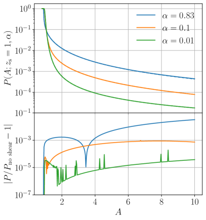
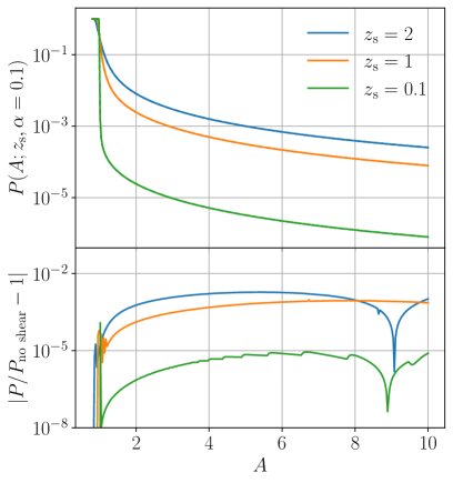
Figure 12: Final CDF of the amplification, $P(A;z_{\mathrm{s}},\alpha)\equiv\mathrm{Prob}(>A|z_{\mathrm{s}};\alpha)$, once marginalised over the line-of-sight convergence $\bar{\kappa}_{\mathrm{os}}$. Left: dependence in the fraction $\alpha$ of compact objects for $z_{\mathrm{s}}=1$. Right: dependence in the source redshift $z_{\mathrm{s}}$, for $\alpha=0.1$. Upper panels indicate both the exact result (solid lines) and the case where the effect of shear is neglected therein, i.e., for $\mathcal{K}=1$ (dashed lines). The solid and dashed lines are superimposed – their relative difference is depicted in the bottom panels; the rapidly oscillating features are non-physical artefacts due to numerical integration.

The final amplification CDF is depicted in fig. 12, for different values of the fraction $\alpha$ of compact objects and of the source redshift $z_{\mathrm{s}}$. As expected, the probability of high amplifications increases with both $\alpha$ and $z_{\mathrm{s}}$, because the optical depth $\tau$ increases with both parameters. For a source at $z_{\mathrm{s}}=1$, the probability that it is amplified by a factor larger than two is $1.6\text{\,}\mathrm{\char 37\relax}$ if all the DM ($83\text{\,}\mathrm{\char 37\relax}$ of the total matter) in the Universe is made of compact objects. This probability falls to $0.23\text{\,}\mathrm{\char 37\relax}$ if $10\text{\,}\mathrm{\char 37\relax}$ of matter is compact, and to $0.056\text{\,}\mathrm{\char 37\relax}$ if only $1\text{\,}\mathrm{\char 37\relax}$ of the matter is compact.

The upper panels of fig. 12 show both the exact $P(A;z_{\mathrm{s}},\alpha)$ and the case where microshear is neglected, which corresponds to setting $\mathcal{K}=1$ in eq. 4.17,

$$P_{\mathrm{no\ shear}}(A;z_{\mathrm{s}},\alpha,\bar{\kappa}_{\mathrm{os}}) \equiv 1-\exp\left[-\frac{2\tau}{1-\kappa_{\mathrm{os}}}\int_{A/A_{\mathrm{min}}}^{\infty}\frac{\mathrm{d}X}{\left(X^{2}-1\right)^{3/2}}\right]$$ (4.19)

$$=1-\exp\left[-\frac{2\tau}{1-\kappa_{\mathrm{os}}}\left(\frac{A}{\sqrt{A^{2}-A_{\mathrm{min}}^{2}}}-1\right)\right].$$ (4.20)

The associated curves are essentially indistinguishable by eye; their relative difference, $|P/P_{\mathrm{no\ shear}}-1|$, is shown in the bottom panels of fig. 12 and is sub-percent for $A<6$. Of course, due to the behaviour of the function $\mathcal{K}(x)$, larger amplifications ($A\sim 1/\tau$) are expected to be affected more significantly by the microshear. But in practice such high amplifications are so rare that they have no observational relevance. Hence, the main take-home message of this subsection is that the effect of shear is negligible in the statistics of extragalactic microlensing. This implies that, for practical purposes, one may safely use the simple no-shear expression (4.20) for $P(A;z_{\mathrm{s}},\alpha;\bar{\kappa}_{\mathrm{os}})$. Such a conclusion could hardly have been guessed from the beginning. The external shear is known to be a crucial parameter in the modelling of strong lenses (e.g. [80]), and fig. 7 shows that it generally has a significant impact on the amplification cross section. But since the effect shows up around amplifications $A\sim 1/\tau$, and that the amplification PDF is already low for $A\gtrsim 1/\tau$, the net integrated effect on $P(A)$ ends up being negligible for interesting values of $A$.

4.4 Comparison with Zumalacárregui & Seljak

In ref. [38] (hereafter ZS17), Zumalacárregui & Seljak have set constraints on the fraction of extragalactic compact objects that would produce a microlensing signal in the supernova data. For that purpose, they used a phenomenological model for the amplification statistics. It is worth comparing the predictions of that model to our approach in order to evaluate what one may call theoretical systematics on any analysis of supernova microlensing.

ZS17’s model, based on earlier developments by Seljak & Holz [35] and Metcalf & Silk [34, 37], is expressed in terms of a shifted magnification $\mu$, such that $1+\mu$ represents the magnification of an image with respect to its empty-beam counterpart, i.e., if that image were seen through an empty universe. It is related to our amplification $A$ as

$$1+\mu=(1+\Delta_{\mathrm{os}})^{2}\,A\ ,$$ (4.21)

where $\Delta_{\mathrm{os}}$ is the same as defined in eq. 2.9. With such conventions, $\mu=0$ corresponds to $A=(1+\Delta_{\mathrm{os}})^{-2}$, which is indeed the empty-beam case. The distribution of $\mu$ is then designed by assuming that $\mu$ can be written as the sum $\mu=\mu_{\mathrm{s}}+\mu_{\mathrm{c}}$ of a weak-lensing contribution from the smooth matter, $\mu_{\mathrm{s}}$, and a microlensing contribution from compact objects, $\mu_{\mathrm{c}}$.

The smooth part is written as $\mu_{\mathrm{s}}=(1-\alpha)\bar{\mu}$, where $\bar{\mu}$ would be the magnification in the absence of compact objects. Note that this is quite similar to our approach described in subsubsec. 3.2.2, except that we have worked with convergences rather than shifted magnifications. In ZS17, the statistics of $\bar{\mu}$ are obtained using the TurboGL code [81, 82].

The statistics of microlensing part, $\mu_{\mathrm{c}}$, are based on an empirical model originally used by Rauch to fit ray-shooting simulations in ref. [83],

$$p_{\mathrm{R}}(\mu_{\mathrm{c}};\bar{\mu}_{\mathrm{c}})=N\left[\frac{1-\mathrm{e}^{-\mu_{\mathrm{c}}/\Delta\mu}}{(1+\mu_{\mathrm{c}})^{2}-1}\right]^{3/2},$$ (4.22)

where $N$ and $\Delta\mu$ are two functions of $\bar{\mu}_{\mathrm{c}}$ that are chosen so as to ensure that $p_{\mathrm{R}}$ is normalised to 1 and with expectation value $\left\langle\mu_{\mathrm{c}}\right\rangle=\bar{\mu}_{\mathrm{c}}$. This value is set to be $\bar{\mu}_{\mathrm{c}}=\alpha\bar{\mu}$ by the magnification theorem [61], and plays a role comparable to the optical depth $\tau$ in our approach.

In such conditions, ZS17’s model for the PDF of the magnification $\mu=\mu_{\mathrm{c}}+\mu_{\mathrm{s}}$ reads

$$p_{\mathrm{ZS17}}(\mu;z_{\mathrm{s}})=\int_{0}^{\infty}\mathrm{d}\bar{\mu}\;p_{\mathrm{TurboGL}}(\bar{\mu};z_{\mathrm{s}})\,p_{\mathrm{R}}[\mu-(1-\alpha)\bar{\mu};\alpha\bar{\mu}]\ ,$$ (4.23)

which undoubtedly has the advantage of simplicity. Figure 13 shows a comparison between the predictions of our model with those of ZS17’s model, in the case of point-like sources for simplicity. Compared to our approach, ZS17’s model tends to overestimate by more than $10\text{\,}\mathrm{\char 37\relax}$ the large-amplification events for high values of $\alpha$; for low values of $\alpha$, on the contrary, it tends to underestimate them by more than $100\text{\,}\mathrm{\char 37\relax}$. Coincidentally, both models nearly agree (up to a few percent) for $\alpha=0.35$, which turns out to be the maximum fraction of compact objects allowed at $95\text{\,}\mathrm{\char 37\relax}$ confidence level in ZS17. Since $P_{\mathrm{ZS17}}(A)>P(A)$ for smaller values of $\alpha$, this suggest that conducting an analysis similar to ZS17’s with our model for amplification statistics would yield slightly weaker constraints on $\alpha$. Such an analysis is beyond the scope of this article, but the present results show that theoretical systematics can generally reach $100\text{\,}\mathrm{\char 37\relax}$ for extragalactic microlensing.

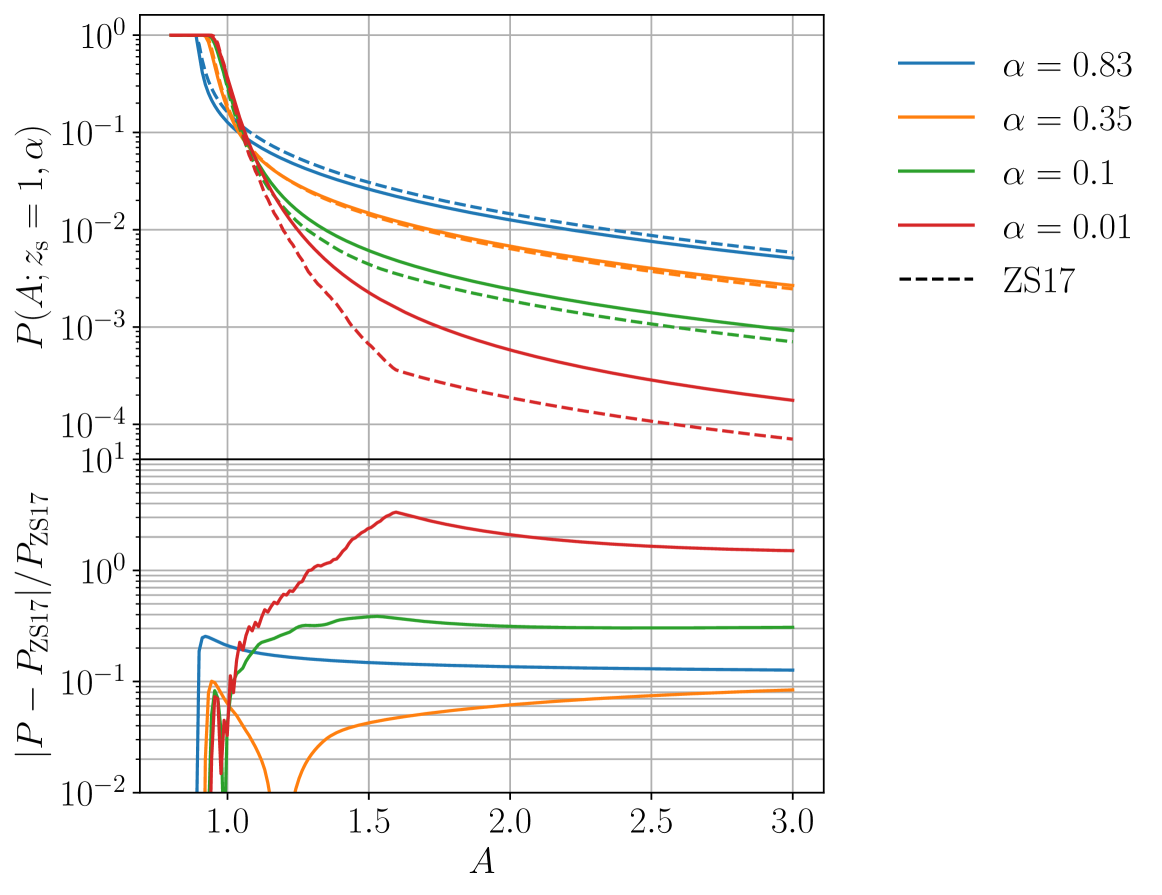
Figure 13: Comparison of our model for the amplification CDF (solid lines) and the phenomenological model used in ZS17 [38] (dashed lines), for point-like sources at $z_{\rm s}=1$ and different values of the fraction of compact objects $\alpha$.

5 Extended sources

So far we have considered point-like sources, but the finite size of real light sources is known to have significant effects on the amplification distribution. As a rule of thumb, if a source has an unlensed angular size $\sigma$, then it smoothes out the amplification map obtained in the point-source case on the angular scale $\sigma$ – see e.g. fig. 13 of ref. [57] for illustration. This implies that the effect of small structures, i.e. lenses with small Einstein radii, is suppressed. In this subsection, we show how to add finite-source corrections to the amplification distributions derived in the previous sections.

5.1 Extended-source corrections on an isolated point lens

We have seen in subsubsec. 3.2.3 that the problem of a point lens with tidal corrections can be conveniently phrased as an equivalent point lens with a single effective shear correction. Besides, the analysis leading to fig. 12 shows that the effect of shear is statistically negligible in the point-source case. Since the extended-source case is deduced from the point-source case by a smoothing of its amplification map, if the effect of shear is small in the latter, it must also be small in the former. Hence, in all the remainder of this section we shall neglect the shear, so the equivalent lens is a mere unperturbed point lens,

$$\tilde{\bm{\beta}}=\tilde{\bm{\theta}}-\frac{\tilde{\theta}_{\mathrm{E}}^{2}}{\tilde{\bm{\theta}}}\ ,$$ (5.1)

where the twiddled quantities are expressed in terms of the original ones in eqs. 3.13, 3.14 and 3.15, all the shears being set to zero.

Let us now consider a source shaped as a disk with angular radius $\sigma$, and whose surface brightness is homogeneous within the disk. Since we are neglecting the shear, the source shape is still a disk in the twiddled world, with radius $\tilde{\sigma}=(1-\kappa_{\mathrm{od}})(1-\kappa_{\mathrm{ds}})^{-1}(1-\kappa_{\mathrm{os}})^{-1}\sigma$. The amplification profile of such a homogeneous disk source by a point lens was derived in ref. [84]. If $\tilde{\beta}$ denotes, in the twiddled world, the angle between the centre of the source and the main lens, we define the reduced impact parameter as $\tilde{u}\equiv\tilde{\beta}/\tilde{\theta}_{\mathrm{E}}$ and the reduced source’s radius $\tilde{r}\equiv\tilde{\sigma}/\tilde{\theta}_{\mathrm{E}}$; the amplification profile then reads

$$\tilde{A}(\tilde{u},\tilde{r})=\frac{\tilde{u}+\tilde{r}}{2\pi\tilde{r}^{2}}\sqrt{4+(\tilde{u}-\tilde{r})^{2}}\,\mathrm{E}(m)-\frac{\tilde{u}-\tilde{r}}{2\pi\tilde{r}^{2}}\frac{8+(\tilde{u}^{2}-\tilde{r}^{2})}{\sqrt{4+(\tilde{u}-\tilde{r})^{2}}}\,\mathrm{F}(m)\\ +\frac{2(\tilde{u}-\tilde{r})^{2}}{\pi\tilde{r}^{2}(\tilde{u}+\tilde{r})}\frac{1+\tilde{r}^{2}}{\sqrt{4+(\tilde{u}-\tilde{r})^{2}}}\,\Pi(n,m)\ ,$$ (5.2)

where

$$n\equiv\frac{4\tilde{u}\tilde{r}}{(\tilde{u}+\tilde{r})^{2}}\ ,\qquad m\equiv\frac{4n}{4+(\tilde{u}-\tilde{r})^{2}}\ ,$$ (5.3)

and the functions $\mathrm{F}$, $\mathrm{E}$ and $\Pi$ are the complete elliptic integrals of the first, second and third type, respectively, in Wolfram’s convention for elliptic integrals. The maximum amplification is obtained when $\tilde{u}=0$ and reads

$$\tilde{A}_{\mathrm{max}}(\tilde{r})\equiv\tilde{A}(0,\tilde{r})=\sqrt{1+\frac{4}{\tilde{r}^{2}}}\ ,$$ (5.4)

which goes to infinity as the source becomes very small ($\tilde{r}\to 0$). More generally, the entire amplification profile of the point-source case (2.2) is recovered in that limit. The left panel of fig. 14 illustrates the amplification profile for several values of $\tilde{r}$.

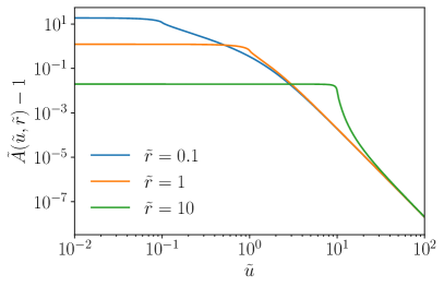
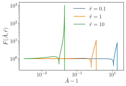
Figure 14: Finite-source corrections for the amplification of a homogeneous disk source with angular radius $\tilde{\sigma}=\tilde{r}\tilde{\theta}_{\mathrm{E}}$ by a point lens with Einstein radius $\tilde{\theta}_{\mathrm{E}}$. Left: Amplification profile $\tilde{A}$ as a function of the reduced impact parameter $\tilde{u}=\tilde{\beta}/\tilde{\theta}_{\mathrm{E}}$. The larger the source, the smoother the profile and the smaller the maximum amplification. Right: Correction factor to the differential amplification cross section, $F\equiv\tilde{\Omega}_{\tilde{\sigma}}/\tilde{\Omega}_{0}$, for the same values of $\tilde{r}$.

In the next subsubsections, we proceed with the calculation of the amplification probability in the presence of finite-source corrections. This calculation will closely follow the point-source case: amplification cross-section; strongest-lens approximation; and marginalisation over the mesoscopic cone.

5.2 Amplification cross section of an isolated lens

With an extended source, the amplification profile changes from eq. 2.2 to eq. 5.2, so the differential cross section amplification must change as well. In particular, since $\tilde{A}\leq\tilde{A}_{\mathrm{max}}(\tilde{r})$, we must have $\tilde{\Omega}_{\tilde{\sigma}}(\tilde{A}>\tilde{A}_{\mathrm{max}})=0$. Thanks to the axial symmetry of the amplification profile, just like the point-lens case, we have

$$\tilde{\Omega}_{\tilde{\sigma}}(\tilde{A})=2\pi\tilde{\beta}(\tilde{A},\tilde{r})\left|\frac{\partial\tilde{\beta}}{\partial{\tilde{A}}}\right|=\pi\tilde{\theta}_{\mathrm{E}}^{2}\left|\frac{\partial\tilde{u}^{2}}{\partial\tilde{A}}\right|,$$ (5.5)

except that now $\tilde{u}(\tilde{A},\tilde{r})$ is the inverse of eq. 5.2 at fixed $\tilde{r}$, which cannot be done analytically.

For later convenience, we introduce the finite-source factor $F$ as the ratio between the finite-source and point-source amplification cross sections,

$$F(\tilde{A},\tilde{r})\equiv\frac{\tilde{\Omega}_{\tilde{\sigma}}(\tilde{A})}{\tilde{\Omega}_{0}(\tilde{A})}=\frac{\partial\tilde{\beta}^{2}}{\partial\tilde{A}}\,\frac{\mathrm{d}\tilde{A}}{\mathrm{d}\tilde{\beta}_{0}^{2}}\ .$$ (5.6)

This way, finite-source corrections are fully encapsulated in a single function, just like shear corrections were encapsulated in the function $k$ in subsec. 3.3. A significant difference, however, is that the function $F$ has two variables while $k$ had only one, which makes the analysis technically harder. The right panel of fig. 14 shows three examples of $\tilde{A}\mapsto F(\tilde{A},\tilde{r})$, for $\tilde{r}=0.1,1,10$. As expected, for low amplifications $F\approx 1$, which translates the fact that far from the lens, the finiteness of the source has essentially no effect. For larger amplifications, the cross section is enhanced for $\tilde{A}\lesssim\tilde{A}_{\mathrm{max}}(\tilde{r})$ and then suddenly drops to zero beyond.

The amplification cross section in the original problem (non-twiddled world) is obtained from $\tilde{\Omega}(\tilde{A})$ similarly to subsubsec. 3.3.2. The calculation uses that, in terms of the original quantities, $\tilde{r}=\sqrt{A_{\mathrm{min}}}\,\sigma/\vartheta_{\mathrm{E}}$. The final result is

$$\Omega_{\sigma}(A)=2\pi\vartheta_{\mathrm{E}}^{2}\,F\left(\frac{A}{A_{\mathrm{min}}},\sqrt{A_{\mathrm{min}}}\,\frac{\sigma}{\vartheta_{\mathrm{E}}}\right)\frac{A_{\mathrm{min}}^{2}}{(A^{2}-A_{\mathrm{min}}^{2})^{3/2}}\ .$$ (5.7)

5.3 Amplification probabilities with extended sources

Just like in the point-lens case, the amplification PDF for one lens in a mesoscopic cone with half angle $\Theta$ reads

$$p_{1}(A;\sigma)=\frac{1}{\pi\Theta^{2}}\int\mathrm{d}m\,\mathrm{d}\chi\,\;p(m,\chi)\,\Omega_{\sigma}(A;m,\chi)\ .$$ (5.8)

Substituting eq. 5.7 and $p(m,\chi)=(3\chi^{2}/\chi_{\mathrm{s}}^{3})\,p(m)$, we may again gather all the finite-source corrections within a single function as

$$p_{1}(A;\sigma)=\frac{2\left\langle\vartheta_{\mathrm{E}}^{2}\right\rangle}{\Theta^{2}}\,\frac{A_{\mathrm{min}}^{2}}{(A^{2}-A_{\mathrm{min}}^{2})^{3/2}}\,\mathcal{F}\left(\frac{A}{A_{\mathrm{min}}},\sigma,\kappa_{\mathrm{os}}\right)\ ,$$ (5.9)

with $\mathcal{F}\equiv\left\langle\vartheta_{\mathrm{E}}^{2}F\right\rangle/\left\langle\vartheta_{\mathrm{E}}^{2}\right\rangle$, that is, explicitly,

$$\mathcal{F}(X,\sigma,\kappa_{\mathrm{os}})=\frac{\int_{0}^{\chi_{\mathrm{s}}}\frac{\mathrm{d}\chi}{a(\chi)}\;\frac{1-\kappa_{\mathrm{ds}}}{1-\kappa_{\mathrm{od}}}\,\chi(\chi_{\mathrm{s}}-\chi)\int\mathrm{d}m\;\frac{m}{\left\langle m\right\rangle}\,F\left[X,\sigma\sqrt{\frac{1-\kappa_{\mathrm{od}}}{(1-\kappa_{\mathrm{os}})(1-\kappa_{\mathrm{ds}})}\frac{a(\chi)\chi\chi_{\mathrm{s}}}{4Gm(\chi_{\mathrm{s}}-\chi)}}\right]}{\int_{0}^{\chi_{\mathrm{s}}}\frac{\mathrm{d}\chi}{a(\chi)}\;\frac{1-\kappa_{\mathrm{ds}}}{1-\kappa_{\mathrm{od}}}\,\chi(\chi_{\mathrm{s}}-\chi)}\ ,$$ (5.10)

where $X=A/A_{\mathrm{min}}$. Equation 5.9 is formally quite similar to eq. 4.11, which was the case of point-like sources with external shear. However, here the correction factor $\mathcal{F}(X,\sigma,\kappa_{\mathrm{os}})$ has three variables, instead of one for the function $\mathcal{K}(x)$ of eq. 4.11

Figure 15 shows examples of the $\mathcal{F}$ function for two types of sources (SNe and QSOs) at $z_{\mathrm{s}}=1$, in the case where all the compact objects have the same mass $m$; we have set all the convergences to zero for simplicity. As expected, $\mathcal{F}$ being a smoothed version of $F$, it preserves some of its features; in particular, the amplification probability is suppressed beyond a critical value of $X=A/A_{\mathrm{min}}$. For a given source size $\sigma$, the lower the deflectors’ mass $m$, the larger the values of $r$ and hence the smaller the critical amplification; this is apparent in both panels of fig. 15, where the curves are displaced to the left as $m$ decreases. For relatively large values of the deflectors’ mass, $\mathcal{F}(X,\sigma)$ is almost self-similar. As expected, the lens mass required to allow large amplifications to happen is much larger for QSOs than for SNe, because the latter is much closer to a point source than the former.

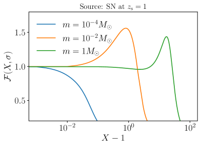
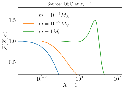
Figure 15: Examples of the extended-source correction factor $\mathcal{F}(X,\sigma,\kappa_{\mathrm{os}}=0)$ involved in eq. 5.9, for two different kind of sources at $z_{\mathrm{s}}=1$, in the case where all the compact objects have the same mass $m$. Left: The sources are SNe, with physical radius $300\text{\,}\mathrm{AU}$, i.e. $\sigma_{\mathrm{SN}}=\mathcal{O}(10^{-13})$ rad at $z_{\mathrm{s}}=1$. Right: The sources are QSOs, with physical radius 4 light days, i.e. $\sigma_{\mathrm{QSO}}=\mathcal{O}(10^{-9})$ rad at $z_{\mathrm{s}}=1$.

Finally, the total amplification CDF, produced by an infinite population of lenses in the mesoscopic cone, is derived from eq. 5.9 following the exact same method as in subsec. 4.2, i.e. in the framework of the strongest-perturbed lens approximation. The result is

$$P(A;\sigma,z_{\mathrm{s}},\alpha,\bar{\kappa}_{\mathrm{os}})=1-\exp\left\{\frac{-2\tau}{1-\kappa_{\mathrm{os}}}\int_{A/A_{\mathrm{min}}}^{\infty}\frac{\;\mathrm{d}X}{(X^{2}-1)^{3/2}}\,\mathcal{F}(X,\sigma,\kappa_{\mathrm{os}})\right\},$$ (5.11)

with $\tau=\alpha(\Delta_{\mathrm{os}}+\bar{\kappa}_{\mathrm{os}})$, $\kappa_{\mathrm{os}}=(1-\alpha)\bar{\kappa}_{\mathrm{os}}-\alpha\Delta_{\mathrm{os}}$ and $A_{\mathrm{min}}=(1-\kappa_{\mathrm{os}})^{-2}$. Averaging over the mesoscopic cone is obtained by marginalising over $\bar{\kappa}_{\mathrm{os}}$, as discussed in subsec. 4.3.

Examples of $P(A;z_{\mathrm{s}},\alpha,\bar{\kappa}_{\mathrm{os}},\sigma)$ for various values of its parameters are depicted in fig. 16; we fixed $\bar{\kappa}_{\mathrm{os}}=0$ for simplicity. Compared to the point-source case, the amplification probability is slightly enhanced near some critical value that depends on the lens masses, source redshift and size, after what it gets quickly suppressed. As expected from our analysis of the function $\mathcal{F}$, finite-source effects are stronger as the source size increases and the mass of the compact objects decreases.

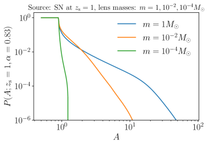
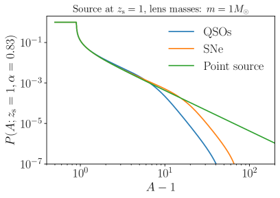
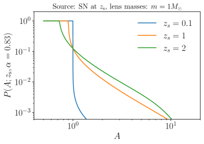
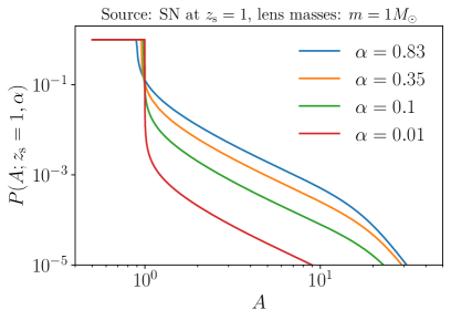
Figure 16: Examples of the amplification CDF $P(A;\sigma,z_{\mathrm{s}},\alpha,\bar{\kappa}_{\mathrm{os}})$ with extended sources, as given by eq. 5.11, for a line of sight with $\bar{\kappa}_{\mathrm{os}}=0$. Top left: Varying the mass $m$ of the compact objects. Top right: Changing the source type, namely point sources, SNe [physical radius $300\text{\,}\mathrm{AU}$ i.e. $\sigma_{\mathrm{SN}}=\mathcal{O}(10^{-13})$ at $z_{\mathrm{s}}=1$], and QSOs [physical radius 4 light days i.e. $\sigma_{\mathrm{QSO}}=\mathcal{O}(10^{-9})$ at $z_{\mathrm{s}}=1$]. Bottom left: Varying the source redshift $z_{\mathrm{s}}$. Bottom right: Varying the fraction $\alpha$ of compact objects.

6 Conclusion

Extragalactic microlensing is a potentially powerful probe of the nature of dark matter (DM). In particular, a handful of past studies have used supernova microlensing to set constraints on the fraction of intergalactic DM that could be made of compact objects. Those analyses relied on a simple phenomenological modelling of the microlensing amplification statistics, which did not account for the coupling between the main deflector responsible for the amplification and its environment – the other lenses and the large-scale cosmic structures. Such an approximation is expected to be valid in the limit of very low optical depths, and for lines of sight that are representative of the mean homogeneous and isotropic model.

In this work, we started assessing the validity of the very-low-optical-depth assumption, and found that for observationally interesting values of the microlensing amplification, relevant optical depths are low to mild ($\tau\lesssim 0.1$). This first result, together with the known fact that environmental effects are generally non-negligible in strong lensing, suggests that environmental and line-of-sight corrections may be significant in extragalactic microlensing. Hence, they must be taken into account in order to accurately predict the probability of microlensing amplification by a cosmic population of compact objects.

We have derived, from first principles, an expression for the amplification probability that we expect to be valid up to mild optical depths. Our approach, which may be referred to as the “strongest perturbed lens model”, consistently accounts for: (i) the external convergences due to overdensities or underdensities in the smooth matter distribution along the line of sight; and (ii) the external shears produced by the large-scale structure and the lenses near the line of sight. This result and its derivation constitute the main focus of the article. The derivation was performed in the case of point-like sources of light, but we also explicitly derived the extended-source corrections for completeness. In numerical illustrations, the statistical distributions of the line-of-sight convergences and shears were extracted from ray tracing in $N$-body simulations, for which we found interesting fitting functions.

From this new model of microlensing amplification probabilities, two conclusions turn out to be particularly noteworthy. First, in observationally relevant situations, the effect of external shear (both due to the large-scale structure and to compact objects near the line of sight) is statistically negligible – corrections are at most on the order of a part in a thousand. Second, however, the predictions of our model are still quantitatively discrepant from the literature, with relative differences larger than $100\text{\,}\mathrm{\char 37\relax}$ in some cases. Such differences might be explained from our non-linear treatment of the external convergences and our careful embedding of microlenses within the cosmic large-scale structure. This result emphasises the crucial importance of an elaborate theoretical modelling of amplification statistics in order to extract accurate constraints on the fraction of compact objects in the Universe.

The next step of this work naturally consists in applying its result to, e.g., SN data similarly to what was done in refs. [35, 34, 37, 38, 87]. This will require an efficient numerical implementation of our model for the amplification probability, which can be technically challenging for extended-source corrections. Application to data requires to properly deal with their outliers, in order to distinguish between lensed and intrinsically anomalous SNe.

Appendix A Weak-lensing statistics with RayGalGroupSims

This appendix is dedicated to our analysis of the statistics of weak-lensing convergence and shear from a numerical simulation. Specifically, we have used results from a dark-matter-only simulation performed with the $N$-body code RAMSES [88, 89]. The simulation has been performed with the best-fit parameters of WMAP-7 [90], a comoving length of $2625h^{-1}~{}\text{Mpc}$ and a particle mass of $1.88\times 10^{10}h^{-1}M_{\odot}$. Fully relativistic ray tracing has been performed through this simulation [64] using the Magrathea library [91, 92]. Healpix maps with various lensing quantities, such as convergence, shear and magnification, are publicly available. We focus here on the PDF of convergence $\bar{\kappa}_{\mathrm{os}}$ and (macro)shear $\bar{\gamma}_{\mathrm{os}}$.

A.1 Convergence

We analysed the PDF of the weak-lensing convergence $\bar{\kappa}_{\mathrm{os}}$ obtained by ray tracing. In the redshift range $z_{\mathrm{s}}<2$, we found that the following ansatz provides a good fit to the data,

$$p(\bar{\kappa}_{\mathrm{os}};z_{\mathrm{s}})=\frac{\mathrm{d}}{\mathrm{d}{\bar{\kappa}_{\mathrm{os}}}}\exp\left\{-\left[\frac{\Delta\kappa(z_{\mathrm{s}})}{\bar{\kappa}_{\mathrm{os}}-\kappa_{0}(z_{\mathrm{s}})}\right]^{\nu(z_{\mathrm{s}})}+\left[\frac{\Delta\kappa(z_{\mathrm{s}})}{1-\kappa_{0}(z_{\mathrm{s}})}\right]^{\nu(z_{\mathrm{s}})}\right\},$$ (A.1)

where the parameters $\nu$, $\kappa_{0}$ and $\Delta\kappa$ depend on the source redshift $z_{\mathrm{s}}$. Note that eq. A.1 is normalised to 1 for $\bar{\kappa}_{\mathrm{os}}\in[\kappa_{0},1]$ by definition; $\kappa_{0}(z_{\mathrm{s}})<0$ thus denotes the minimum convergence for sources at a redshift $z_{\mathrm{s}}$. Imposing that the convergence averages to $0$ imposes the following constraint between the model parameters,

$$\kappa_{0}=-\Gamma\left[\frac{\nu-1}{\nu}\right]\Delta\kappa\ ,$$ (A.2)

where $\Gamma$ denotes the usual Gamma function. Together with the above, we find that

$$\nu(z_{\mathrm{s}})=2.3\,(1+z_{\mathrm{s}})$$ (A.3)

fits well the data as $\Delta\kappa$ is left as a free parameter. The accuracy of this empirical fit is illustrated in the left panel of fig. 17.

As could be guessed from eq. A.1, $\Delta\kappa$ is related to the variance of the convergence. Specifically, we have

$$\big{\langle}\bar{\kappa}_{\mathrm{os}}^{2}\big{\rangle}=\left[\Gamma\left(\frac{\nu-2}{\nu}\right)-\Gamma^{2}\left(\frac{\nu-1}{\nu}\right)\right]\Delta\kappa^{2}\ .$$ (A.4)

The variance of the convergence significantly depends on the cosmology. In the weak-lensing regime, at linear order and in Limber’s approximation, it is known to read

$$\big{\langle}\bar{\kappa}_{\mathrm{os}}^{2}\big{\rangle}=\int_{0}^{\infty}\frac{\ell\mathrm{d}\ell}{2\pi}\;P_{\kappa}(\ell,z_{\mathrm{s}})\ ,$$ (A.5)

where $P_{\kappa}$ denotes the convergence angular power spectrum, which is directly related to the matter power spectrum [74]. Since the simulation data at our disposal used slightly outdated cosmological parameters, we thus expect the resulting $\big{\langle}\bar{\kappa}_{\mathrm{os}}^{2}\big{\rangle}$ to be outdated as well. In order to circumvent this issue, we estimated $\big{\langle}\bar{\kappa}_{\mathrm{os}}^{2}\big{\rangle}$ from eq. A.5 using camb. For a Planck-2018 cosmology [55], we find that the standard deviation of the convergence is well fit by

$$\sqrt{\big{\langle}\bar{\kappa}_{\mathrm{os}}^{2}\big{\rangle}}=0.0218\left[\left(1+12.6\,z\right)^{0.315}-1\right],$$ (A.6)

as illustrated in the right panel of fig. 17. In practice, we substitute this expression into eq. A.4 to determine $\Delta\kappa(z_{\mathrm{s}})$ for application in this article.

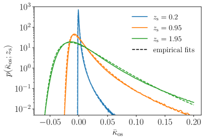
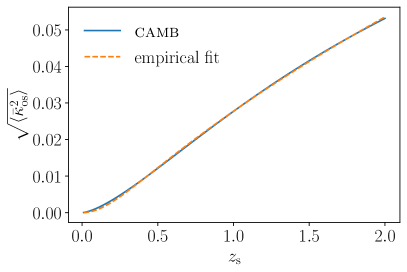
Figure 17: Statistics of the weak-lensing convergence $\bar{\kappa}_{\mathrm{os}}$. Left: comparison between the PDF of the convergence $\bar{\kappa}_{\mathrm{os}}$ obtained from ray tracing in an $N$-body simulation (solid lines) and the ansatz of eq. A.1 (dashed lines), with the constraint (A.2), $\nu(z_{\mathrm{s}})=2.3(1+z_{\mathrm{s}})$ and $\Delta\kappa$ left as a free parameter. Right: standard deviation of the convergence computed from camb with a Planck-2018 cosmology, compared with the empirical fit of eq. A.6.

A.2 Macroshear

In the range of redshift relevant for the present discussion, we find that the conditional PDF for the shear at a fixed convergence, $p(\bar{\gamma}_{\mathrm{os}};\bar{\kappa}_{\mathrm{os}},z_{\mathrm{s}})$, is surprisingly well fit by a two-dimensional Gaussian distribution,

$$p(\bar{\gamma}_{\mathrm{os}};\bar{\kappa}_{\mathrm{os}},z_{\mathrm{s}})\,\mathrm{d}^{2}\bar{\gamma}_{\mathrm{os}}=\frac{1}{2\pi\sigma^{2}(\bar{\kappa}_{\mathrm{os}},z_{\mathrm{s}})}\exp\left[-\frac{|\bar{\gamma}_{\mathrm{os}}|^{2}}{2\sigma^{2}(\bar{\kappa}_{\mathrm{os}},z_{\mathrm{s}})}\right]\mathrm{d}^{2}\bar{\gamma}_{\mathrm{os}}\ .$$ (A.7)

Since the Universe is statistically isotropic, there is no preferred orientation for the complex shear, and hence the conditional PDF of its magnitude takes the form

$$\mathcal{P}(|\bar{\gamma}_{\mathrm{os}}|;\bar{\kappa}_{\mathrm{os}},z_{\mathrm{s}}) =2\pi|\bar{\gamma}_{\mathrm{os}}|\,p(\bar{\gamma}_{\mathrm{os}};\bar{\kappa}_{\mathrm{os}},z_{\mathrm{s}})$$ (A.8)

$$=\frac{|\bar{\gamma}_{\mathrm{os}}|}{\sigma^{2}(\bar{\kappa}_{\mathrm{os}},z_{\mathrm{s}})}\exp\left[-\frac{|\bar{\gamma}_{\mathrm{os}}|^{2}}{2\sigma^{2}(\bar{\kappa}_{\mathrm{os}},z_{\mathrm{s}})}\right]$$ (A.9)

$$=\frac{\mathrm{d}}{\mathrm{d}|\bar{\gamma}_{\mathrm{os}}|}\exp\left[-\frac{|\bar{\gamma}_{\mathrm{os}}|^{2}}{2\sigma^{2}(\bar{\kappa}_{\mathrm{os}},z_{\mathrm{s}})}\right].$$ (A.10)

Figure 18 shows a comparison between the numerical data and the ansatz (A.10) for $z_{\mathrm{s}}=0.95$; at that redshift we find the empirical expression $\sigma(\bar{\kappa}_{\mathrm{os}},z_{\mathrm{s}}=0.95)=0.01+0.26\,\bar{\kappa}_{\mathrm{os}}$.

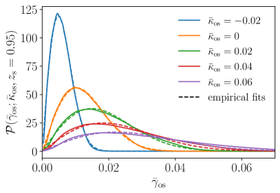
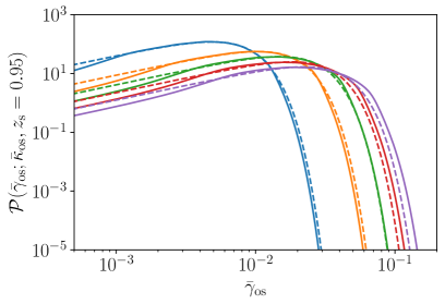
Figure 18: Conditional PDF of the magnitude of weak-lensing shear $|\bar{\gamma}_{\mathrm{os}}|$ at fixed values of the convergence $\bar{\kappa}_{\mathrm{os}}$, for sources at $z_{\mathrm{s}}=0.95$. The figures compare results from simulations (solid lines) with the ansatz of eq. A.10 (dashed lines). Left: linear scale. Right: logarithmic scale.

Appendix B Derivation of the microshear distribution

This appendix is dedicated to the derivation of the distribution of the effective reduced microshear that was given in eq. 4.4.

B.1 PDF of a sum of complex shears

Consider $N$ randomly distributed lenses $\ell$, each one producing a complex shear $s_{\ell}\in\mathbb{C}$. The total shear is the sum of all those contributions,

$$s=\sum_{\ell=1}^{N}s_{\ell}\ .$$ (B.1)

The PDF of $s$ is, therefore, the convolution product of the $N$ PDFs of the individual shears. Assuming – without loss of generality – that the $N$ lenses are indistinguishable and have identical statistical properties, we have

$$p_{N}(s)=\underbrace{(p_{1}\star\ldots\star p_{1})}_{\text{$N$ times}}(s)\equiv p_{1}^{\star N}(s)\ ,$$ (B.2)

where a $\star$ denotes a convolution product and $p_{1}$ is the PDF of the shear for $1$ lens, accounting for the randomness of its position, mass, etc. The convolution product is better handled in Fourier space. We define here the Fourier transform in a way that acknowledges the spin-$2$ character of the complex shear,

$$\tilde{p}(q)\equiv\int\mathrm{d}^{2}s\;\mathrm{e}^{-2\mathrm{i}\mathrm{Re}(q^{*}s)}\,p(s)\ ,\qquad p(s)=\int\frac{\mathrm{d}^{2}q}{(2\pi)^{2}}\;\mathrm{e}^{2\mathrm{i}\mathrm{Re}(q^{*}s)}\,\tilde{p}(q)\ ,$$ (B.3)

with $q\in\mathbb{C}$ the Fourier variable dual to $s$; ^∗ denotes complex conjugation and the differential elements are $\mathrm{d}^{2}q=\mathrm{d}q_{1}\mathrm{d}q_{2}$, $\mathrm{d}^{2}s=\mathrm{d}s_{1}\mathrm{d}s_{2}$. We shall also use polar components for both $s=S\mathrm{e}^{2\mathrm{i}\varphi}$ and $q=Q\mathrm{e}^{2\mathrm{i}\psi}$, with $\varphi,\psi\in[0,\pi)$, in which case $\mathrm{d}^{2}s=2S\mathrm{d}S\mathrm{d}\varphi$ and $\mathrm{d}^{2}q=2Q\mathrm{d}Q\mathrm{d}\psi$. In Fourier space with the above convention, eq. B.2 becomes

$$\tilde{p}_{N}(q)=\tilde{p}_{1}^{N}(q)\ .$$ (B.4)

Consider now the case where the lenses are all axisymmetric – this is valid for the application that will eventually interest us, namely point lenses. In that case the PDF of each lens only depends on $S\equiv|s|$,

$$p_{1}(s)\,\mathrm{d}^{2}s=\mathcal{P}_{1}(S)\mathrm{d}S\,\frac{\mathrm{d}\varphi}{\pi}\,\qquad\text{with}\quad\mathcal{P}_{1}(S)\equiv 2\pi S\,p_{1}(S)$$ (B.5)

the PDF of the magnitude of the shear for single lens. The polar angle can be integrated out in the expression of the Fourier transform, which then only depends on $Q=|q|$,

$$\tilde{p}_{1}(Q)=\int_{0}^{\pi}\frac{\mathrm{d}\varphi}{\pi}\int_{0}^{\infty}\mathrm{d}S\;\mathcal{P}_{1}(S)\,\mathrm{e}^{-\mathrm{i}QS\cos 2(\varphi-\psi)}=\int_{0}^{\infty}\mathrm{d}S\;\mathcal{P}_{1}(S)\,J_{0}(QS)\ ,$$ (B.6)

where $J_{0}$ is the zeroth order Bessel function. From the above, we notice that $\tilde{p}_{1}(q)$ may be also be interpreted as the expectation value of that Bessel function for a single lens,

$$\tilde{p}_{1}(Q)=\left\langle J_{0}(QS)\right\rangle_{1}\ ,$$ (B.7)

where $\left\langle\ldots\right\rangle_{1}$ denotes the average over statistics of a single lens.

In the same manner, since $\tilde{p}_{N}(Q)$ does not depend on the polar angle $\psi$ of $q$, we may integrate this angle out in its inverse Fourier transform,

$$p_{N}(S)=\int_{0}^{\infty}\frac{Q\,\mathrm{d}Q}{2\pi}\int_{0}^{\pi}\frac{\mathrm{d}\psi}{\pi}\;\mathrm{e}^{\mathrm{i}QS\cos 2(\psi-\varphi)}\,\tilde{p}_{N}(Q)=\frac{1}{2\pi}\int_{0}^{\infty}\mathrm{d}Q\;Q\,J_{0}(QS)\,\tilde{p}_{N}(Q)\ .$$ (B.8)

The PDF of the sole magnitude $S$ of the sum all all $N$ complex shears is, therefore,

$$\mathcal{P}_{N}(S)=2\pi S\,p_{N}(S)=\int_{0}^{\infty}\mathrm{d}Q\;QS\,J_{0}(QS)\,\tilde{p}_{N}(Q)\ .$$ (B.9)

B.2 Large-$N$ limit

Now consider the setup depicted in fig. 8: the $N\gg 1$ lenses are distributed within a mesoscopic cone with half angle $\Theta$. Now as $\Theta$ is much larger than the typical Einstein radius of the lenses, it quite clear that $\mathcal{P}_{1}(S)$ must approach $\delta(S)$. Since $J_{0}(0)=1$, we conclude that $\tilde{p}_{1}(Q)=\left\langle J_{0}(QS)\right\rangle_{1}\approx 1$. This suggests the following manipulation

$$\tilde{p}_{N}(Q)=\left\langle J_{0}(QS)\right\rangle_{1}^{N}=\left\langle 1+[J_{0}(QS)-1]\right\rangle_{1}^{N}\approx\exp\left[N\left\langle J_{0}(QS)-1\right\rangle_{1}\right]$$ (B.10)

in the large-$N$ limit.

B.3 Application to the effective reduced microshear due to point lenses

The quantity of interest here is the effective reduced microshear, due to the compact objects located near the line of sight of the dominant lens at $\chi$,

$$s\equiv\frac{s_{\mathrm{os}}}{1-\kappa_{\mathrm{os}}}-\frac{s_{\mathrm{od}}}{1-\kappa_{\mathrm{od}}}-\frac{s_{\mathrm{ds}}}{1-\kappa_{\mathrm{ds}}}=\sum_{\ell=1}^{N}s_{\ell}\ ,\qquad s_{\ell}\equiv\frac{4Gm_{\ell}}{(\underline{\beta}_{\ell}^{*})^{2}}\,W(\chi_{\ell}),$$ (B.11)

with

$$W(\chi_{\ell})\equiv(1+z_{\ell})\times\begin{cases}\displaystyle\frac{\chi_{\mathrm{s}}-\chi_{\ell}}{(1-\kappa_{\mathrm{os}})\chi_{\ell}\chi_{\mathrm{s}}}-\frac{\chi_{\mathrm{d}}-\chi_{\ell}}{(1-\kappa_{\mathrm{od}})\chi_{\ell}\chi_{\mathrm{d}}}&\chi_{\ell}\leq\chi_{\mathrm{d}}\\[14.22636pt] \displaystyle\frac{\chi_{\mathrm{s}}-\chi_{\ell}}{(1-\kappa_{\mathrm{os}})\chi_{\ell}\chi_{\mathrm{s}}}-\frac{(\chi_{\ell}-\chi_{\mathrm{d}})(\chi_{\mathrm{s}}-\chi_{\ell})}{(1-\kappa_{\mathrm{ds}})\chi_{\ell}^{2}(\chi_{\mathrm{s}}-\chi_{\mathrm{d}})}&\chi_{\ell}\geq\chi_{\mathrm{d}}\end{cases}$$ (B.12)

where $m_{\ell},z_{\ell},\chi_{\ell}$ denote the mass, redshift, comoving position of lens $\ell$, and $\underline{\beta}_{\ell}$ its complex unlensed angular position with respect to the line of sight; $\chi_{\mathrm{d}},\chi_{\mathrm{s}}$ are the comoving positions of the main deflector and source.

We assume for simplicity that the lenses are uniformly distributed in comoving space, with masses independent of the positions, so that within the mesoscopic cone of fig. 8 we have

$$p(\chi_{\ell},\beta_{\ell},m_{\ell})\,\mathrm{d}\chi_{\ell}\mathrm{d}\beta_{\ell}\mathrm{d}m_{\ell}=\frac{3\chi_{\ell}^{2}\mathrm{d}\chi_{\ell}}{\chi_{\mathrm{s}}^{3}}\,\frac{2\beta_{\ell}\mathrm{d}\beta_{\ell}}{\Theta^{2}}\,p(m_{\ell})\mathrm{d}m_{\ell}\ .$$ (B.13)

In the remainder of this appendix we shall drop the subscript $\ell$ to alleviate notation.

In such conditions, the Fourier transform $\tilde{p}_{1}(Q)$ of the one-lens shear, interpreted as the expectation value of $J_{0}(SQ)$ following eq. B.7 reads

$$\tilde{p}_{1}(Q)=\left\langle J_{0}(SQ)\right\rangle_{1}=\int\frac{\mathrm{d}(\chi^{3})}{\chi_{\mathrm{s}}^{3}}\,\frac{\mathrm{d}(\beta^{2})}{\Theta^{2}}\,p(m)\mathrm{d}m\;J_{0}\left[\frac{4Gm}{\beta^{2}}\,W(\chi)Q\right]-1.$$ (B.14)

We may then perform the change of variable $\beta^{2}\mapsto x=4GmWQ/\beta^{2}$ to get

$$\left\langle J_{0}(SQ)\right\rangle_{1}-1=\frac{4GQ}{\Theta^{2}}\int\mathrm{d}m\;m\,p(m)\int_{0}^{\chi_{\mathrm{s}}}\frac{\mathrm{d}(\chi^{3})}{\chi_{\mathrm{s}}^{3}}\;W(\chi)\int_{4GmWQ/\Theta^{2}}^{\infty}\frac{\mathrm{d}x}{x^{2}}\;[J_{0}(x)-1].$$ (B.15)

In the limit where $\Theta$ is very large, the lower limit in the integral over $x$ can be set to zero, in which case the integral is known,

$$\int_{0}^{\infty}\frac{\mathrm{d}x}{x^{2}}\;[J_{0}(x)-1]=-1\ ,$$ (B.16)

so that

$$\left\langle J_{0}(SQ)\right\rangle_{1}-1\approx-\frac{4G\left\langle m\right\rangle Q}{\Theta^{2}}\int_{0}^{\chi_{\mathrm{s}}}\frac{\mathrm{d}(\chi^{3})}{\chi_{\mathrm{s}}^{3}}\;W(\chi)\ .$$ (B.17)

The last steps of the calculation consist in (i) substituting the above in eq. B.10 and (ii) computing the inverse Fourier transform to get $p_{N}(S)$. Step (i) yields

$$\tilde{p}_{N}(Q)=\mathrm{e}^{-f\tau Q},$$ (B.18)

with the optical depth $\tau=N\left\langle\theta_{\mathrm{E}}^{2}\right\rangle/\Theta^{2}$ corrected by the factor

$$f \equiv\frac{\int_{0}^{\chi_{\mathrm{s}}}\frac{\mathrm{d}(\chi^{3})}{\chi_{\mathrm{s}}^{3}}\;W(\chi)}{\int_{0}^{\chi_{\mathrm{s}}}\frac{\mathrm{d}(\chi^{3})}{\chi_{\mathrm{s}}^{3}}\;\frac{\chi_{\mathrm{s}}-\chi}{a(\chi)\chi\chi_{\mathrm{s}}}}$$ (B.19)

$$=\frac{\int_{0}^{\chi_{\mathrm{d}}}\frac{\mathrm{d}\chi}{a(\chi)}\left[\frac{\chi(\chi_{\mathrm{s}}-\chi)}{(1-\kappa_{\mathrm{os}})\chi_{\mathrm{s}}}-\frac{\chi(\chi_{\mathrm{d}}-\chi)}{(1-\kappa_{\mathrm{od}})\chi_{\mathrm{d}}}\right]+\int_{\chi_{\mathrm{d}}}^{\chi_{\mathrm{s}}}\frac{\mathrm{d}\chi}{a(\chi)}\left[\frac{\chi(\chi_{\mathrm{s}}-\chi)}{(1-\kappa_{\mathrm{os}})\chi_{\mathrm{s}}}-\frac{(\chi-\chi_{\mathrm{d}})(\chi_{\mathrm{s}}-\chi)}{(1-\kappa_{\mathrm{ds}})(\chi_{\mathrm{s}}-\chi_{\mathrm{d}})}\right]}{\int_{0}^{\chi_{\mathrm{s}}}\frac{\mathrm{d}\chi}{a(\chi)}\;\frac{\chi(\chi_{\mathrm{s}}-\chi)}{\chi_{\mathrm{s}}}}.$$ (B.20)

Note that, in the large-$N$ limit, $\tilde{p}_{N}(Q)$ is independent on $N$. The last step (ii) is performed by substituting eq. B.18 into eq. B.9, which finally yields

$$\mathcal{P}_{N}(S)=\int_{0}^{\infty}\mathrm{d}Q\;QS\,J_{0}(QS)\mathrm{e}^{-f\tau Q}=\frac{f\tau S}{\left[(f\tau)^{2}+S^{2}\right]^{3/2}}\ .$$ (B.21)

References

- [1] LIGO Scientific Collaboration and Virgo Collaboration Collaboration, B. A. et al., Gw151226: Observation of gravitational waves from a 22-solar-mass binary black hole coalescence, Phys. Rev. Lett. 116 (Jun, 2016) 241103.
- [2] S. Bird, I. Cholis, J. B. Muñoz, Y. Ali-Haïmoud, M. Kamionkowski, E. D. Kovetz, A. Raccanelli, and A. G. Riess, Did LIGO detect dark matter?, Phys. Rev. Lett. 116 (2016), no. 20 201301, [arXiv:1603.00464].
- [3] S. Clesse and J. García-Bellido, The clustering of massive Primordial Black Holes as Dark Matter: measuring their mass distribution with Advanced LIGO, Phys. Dark Univ. 15 (2017) 142–147, [arXiv:1603.05234].
- [4] M. Sasaki, T. Suyama, T. Tanaka, and S. Yokoyama, Primordial Black Hole Scenario for the Gravitational-Wave Event GW150914, Phys. Rev. Lett. 117 (2016), no. 6 061101, [arXiv:1603.08338]. [Erratum: Phys.Rev.Lett. 121, 059901 (2018)].
- [5] Y. B. Zel’dovich and I. D. Novikov, The Hypothesis of Cores Retarded during Expansion and the Hot Cosmological Model, Soviet Astronomy 10 (Feb., 1967) 602.
- [6] S. Hawking, Gravitationally Collapsed Objects of Very Low Mass, Monthly Notices of the Royal Astronomical Society 152 (04, 1971) 75–78, [https://academic.oup.com/mnras/article-pdf/152/1/75/9360899/mnras152-0075.pdf].
- [7] K. Griest, Galactic Microlensing as a Method of Detecting Massive Compact Halo Objects, ApJ 366 (Jan., 1991) 412.
- [8] B. Carr, F. Kuhnel, and M. Sandstad, Primordial Black Holes as Dark Matter, Phys. Rev. D 94 (2016), no. 8 083504, [arXiv:1607.06077].
- [9] P. J. E. Peebles, Cosmology’s Century: An Inside History of Our Modern Understanding of the Universe. Princeton University Press, 2020.
- [10] B. Paczynski, Gravitational Microlensing at Large Optical Depth, ApJ 301 (Feb., 1986) 503.
- [11] MACHO Collaboration, C. Alcock et al., The MACHO project first year LMC results: The Microlensing rate and the nature of the galactic dark halo, Astrophys. J. 461 (1996) 84, [astro-ph/9506113].
- [12] EROS Collaboration, Limits on galactic dark matter with 5 years of eros smc data, .
- [13] L. Wyrzykowski, J. Skowron, S. Kozłowski, A. Udalski, M. K. Szymański, M. Kubiak, G. Pietrzyński, I. Soszyński, O. Szewczyk, K. Ulaczyk, R. Poleski, and P. Tisserand, The OGLE view of microlensing towards the Magellanic Clouds – IV. OGLE-III SMC data and final conclusions on MACHOs*, Monthly Notices of the Royal Astronomical Society 416 (09, 2011) 2949–2961, [https://academic.oup.com/mnras/article-pdf/416/4/2949/2982628/mnras0416-2949.pdf].
- [14] M. R. S. Hawkins, A new look at microlensing limits on dark matter in the Galactic halo, A&A 575 (Mar., 2015) A107, [arXiv:1503.01935].
- [15] J. Calcino, J. García-Bellido, and T. M. Davis, Updating the MACHO fraction of the Milky Way dark halowith improved mass models, MNRAS 479 (Sept., 2018) 2889–2905, [arXiv:1803.09205].
- [16] G. Sato-Polito, E. D. Kovetz, and M. Kamionkowski, Constraints on the primordial curvature power spectrum from primordial black holes, Phys. Rev. D 100 (Sept., 2019) 063521, [arXiv:1904.10971].
- [17] W. H. Press and J. E. Gunn, Method for Detecting a Cosmological Density of Condensed Objects, ApJ 185 (Oct., 1973) 397–412.
- [18] M. R. S. Hawkins, Gravitational microlensing, quasar variability and missing matter, Nature 366 (Nov., 1993) 242–245.
- [19] M. R. S. Hawkins, The signature of dark matter in quasar light curves, 1998.
- [20] M. R. S. Hawkins and P. Véron, The quasar luminosity function from a variability-selected sample, Monthly Notices of the Royal Astronomical Society 260 (01, 1993) 202–208, [https://academic.oup.com/mnras/article-pdf/260/1/202/18539400/mnras260-0202.pdf].
- [21] P. Schneider, Upper bounds on the cosmological density of compact objects with sub-solar masses from the variability of QSOs., A&A 279 (Nov., 1993) 1–20.
- [22] E. Mediavilla, J. A. Munoz, E. Falco, V. Motta, E. Guerras, H. Canovas, C. Jean, A. Oscoz, and A. M. Mosquera, Microlensing-Based Estimate of the Mass Fraction in Compact Objects in Lens, Astrophys. J. 706 (2009) 1451–1462, [arXiv:0910.3645].
- [23] R. L. Webster, A. M. N. Ferguson, R. T. Corrigan, and M. J. Irwin, Interpreting the Light Curve of Q2237+0305, AJ 102 (Dec., 1991) 1939.
- [24] G. F. Lewis and M. J. Irwin, The statistics of microlensing light curves — II. Temporal analysis, Monthly Notices of the Royal Astronomical Society 283 (10, 1996) 225–240, [https://academic.oup.com/mnras/article-pdf/283/1/225/2849948/283-1-225.pdf].
- [25] H. J. Witt, S. Mao, and P. L. Schechter, On the Universality of Microlensing in Quadruple Gravitational Lenses, ApJ 443 (Apr., 1995) 18.
- [26] P. L. Schechter and J. Wambsganss, Quasar Microlensing at High Magnification and the Role of Dark Matter: Enhanced Fluctuations and Suppressed Saddle Points, ApJ 580 (Dec., 2002) 685–695, [astro-ph/0204425].
- [27] R. B. Metcalf and A. Amara, Small-scale structures of dark matter and flux anomalies in quasar gravitational lenses, Monthly Notices of the Royal Astronomical Society 419 (01, 2012) 3414–3425, [https://academic.oup.com/mnras/article-pdf/419/4/3414/9507595/mnras0419-3414.pdf].
- [28] K. et al., Extreme magnification of a star at redshift 1.5 by a galaxy-cluster lens, 2017.
- [29] W. et al., A highly magnified star at redshift 6.2, Nature 603 (03, 2022) 815–818.
- [30] S. Refsdal, The gravitational lens effect, MNRAS 128 (Jan., 1964) 295.
- [31] S. H. Suyu et al., HOLISMOKES – I. Highly Optimised Lensing Investigations of Supernovae, Microlensing Objects, and Kinematics of Ellipticals and Spirals, Astron. Astrophys. 644 (2020) A162, [arXiv:2002.08378].
- [32] E. V. Linder, P. Schneider, and R. V. Wagoner, Gravitational Lensing Statistics of Amplified Supernovae, ApJ 324 (Jan., 1988) 786.
- [33] K. P. Rauch, Gravitational Microlensing of High-Redshift Supernovae by Compact Objects, ApJ 374 (June, 1991) 83.
- [34] R. B. Metcalf and J. Silk, A Fundamental Test of the Nature of Dark Matter, ApJL 519 (July, 1999) L1–L4, [astro-ph/9901358].
- [35] U. Seljak and D. E. Holz, Limits on the density of compact objects from high redshift supernovae, Astron. Astrophys. 351 (1999) L10, [astro-ph/9910482].
- [36] L. Bergstrom, M. Goliath, A. Goobar, and E. Mortsell, Lensing effects in an inhomogeneous universe, Astron. Astrophys. 358 (2000) 13, [astro-ph/9912194].
- [37] R. B. Metcalf and J. Silk, New Constraints on Macroscopic Compact Objects as Dark Matter Candidates from Gravitational Lensing of Type Ia Supernovae, Phys. Rev. Lett. 98 (Feb., 2007) 071302, [astro-ph/0612253].
- [38] M. Zumalacárregui and U. Seljak, Limits on stellar-mass compact objects as dark matter from gravitational lensing of type Ia supernovae, Phys. Rev. Lett. 121 (2018), no. 14 141101, [arXiv:1712.02240].
- [39] J. Jonsson, T. Dahlen, A. Goobar, C. Gunnarsson, E. Mortsell, and K. Lee, Lensing magnification of supernovae in the GOODS-fields, Astrophys. J. 639 (2006) 991–998, [astro-ph/0506765].
- [40] S. Dhawan, A. Goobar, and E. Mörtsell, The effect of inhomogeneities on dark energy constraints, JCAP 07 (2018) 024, [arXiv:1710.02374].
- [41] J. A. Peacock, Gravitational lenses and cosmological evolution, Monthly Notices of the Royal Astronomical Society 199 (08, 1982) 987–1006, [https://academic.oup.com/mnras/article-pdf/199/4/987/2881476/mnras199-0987.pdf].
- [42] E. L. Turner, J. P. Ostriker, and I. Gott, J. R., The statistics of gravitational lenses : the distributions of image angular separations and lens redshifts., ApJ 284 (Sept., 1984) 1–22.
- [43] C. C. Dyer, Image separation statistics for multiply imaged quasars, ApJ 287 (Dec., 1984) 26–32.
- [44] P. Schneider and A. Weiss, A gravitational lens origin for AGN-variability ? Consequences of micro- lensing., A&A 171 (Jan., 1987) 49–65.
- [45] C. Seitz and P. Schneider, Variability of microlensing light curves I. Autocorrelation method and the calculation of the correlated deflection probability., A&A 288 (Aug., 1994) 1–18.
- [46] R. Nityananda and J. P. Ostriker, Gravitational lensing by stars in a galaxy halo - Theory of combined weak and strong scattering, Journal of Astrophysics and Astronomy 5 (Sept., 1984) 235–250.
- [47] R. Blandford and R. Narayan, Fermat’s Principle, Caustics, and the Classification of Gravitational Lens Images, ApJ 310 (Nov., 1986) 568.
- [48] M. H. Lee and D. N. Spergel, An Analytical Approach to Gravitational Lensing by an Ensemble of Axisymmetric Lenses, ApJ 357 (July, 1990) 23.
- [49] S. Mao, Gravitational Microlensing by a Single Star plus External Shear, ApJ 389 (Apr., 1992) 63.
- [50] L. Kofman, N. Kaiser, M. H. Lee, and A. Babul, Statistics of Gravitational Microlensing Magnification. I. Two-dimensional Lens Distribution, ApJ 489 (Nov., 1997) 508–521, [astro-ph/9608138].
- [51] M. H. Lee, A. Babul, L. Kofman, and N. Kaiser, Statistics of Gravitational Microlensing Magnification. II. Three-dimensional Lens Distribution, ApJ 489 (Nov., 1997) 522–542.
- [52] R. Kayser, S. Refsdal, and R. Stabell, Astrophysical applications of gravitational micro-lensing., A&A 166 (Sept., 1986) 36–52.
- [53] J. Wambsganss, Probability Distributions for the Magnification of Quasars due to Microlensing, ApJ 386 (Feb., 1992) 19.
- [54] G. F. Lewis and M. J. Irwin, The statistics of microlensing light curves - I. Amplification probability distributions, MNRAS 276 (Sept., 1995) 103–114, [astro-ph/9504018].
- [55] Planck Collaboration, N. Aghanim et al., Planck 2018 results. VI. Cosmological parameters, Astron. Astrophys. 641 (2020) A6, [arXiv:1807.06209]. [Erratum: Astron.Astrophys. 652, C4 (2021)].
- [56] P. Schneider, J. Ehlers, and E. E. Falco, Gravitational Lenses. Springer Berlin, Heidelberg, 1992.
- [57] P. Fleury and J. García-Bellido, On simple analytic models of microlensing amplification statistics, Phys. Dark Univ. 29 (2020) 100567, [arXiv:1907.05163].
- [58] J. A. Peacock, Flux conservation and random gravitational lensing, MNRAS 223 (Nov., 1986) 113–128.
- [59] S. Weinberg, Apparent Luminosities in a Locally Inhomogeneous Universe, .
- [60] T. W. B. Kibble and R. Lieu, Average Magnification Effect of Clumping of Matter, ApJ 632 (Oct., 2005) 718–726, [astro-ph/0412275].
- [61] O. Wucknitz, From planes to spheres: about gravitational lens magnifications, MNRAS 386 (May, 2008) 230–244, [arXiv:0801.3758].
- [62] M.-A. Breton and P. Fleury, Theoretical and numerical perspectives on cosmic distance averages, A&A 655 (Nov., 2021) A54, [arXiv:2012.07802].
- [63] Y. B. Zel’dovich, Observations in a Universe Homogeneous in the Mean, Sov. Astron. Lett. 8 (Aug., 1964) 13.
- [64] M.-A. Breton, Y. Rasera, A. Taruya, O. Lacombe, and S. Saga, Imprints of relativistic effects on the asymmetry of the halo cross-correlation function: from linear to non-linear scales, Mon. Not. Roy. Astron. Soc. 483 (2019), no. 2 2671–2696, [arXiv:1803.04294].
- [65] A. Conley, J. Guy, M. Sullivan, N. Regnault, P. Astier, C. Balland, S. Basa, R. G. Carlberg, D. Fouchez, D. Hardin, I. M. Hook, D. A. Howell, R. Pain, N. Palanque-Delabrouille, K. M. Perrett, C. J. Pritchet, J. Rich, V. Ruhlmann-Kleider, D. Balam, S. Baumont, R. S. Ellis, S. Fabbro, H. K. Fakhouri, N. Fourmanoit, S. González-Gaitán, M. L. Graham, M. J. Hudson, E. Hsiao, T. Kronborg, C. Lidman, A. M. Mourao, J. D. Neill, S. Perlmutter, P. Ripoche, N. Suzuki, and E. S. Walker, Supernova Constraints and Systematic Uncertainties from the First Three Years of the Supernova Legacy Survey, ApJS 192 (Jan., 2011) 1, [arXiv:1104.1443].
- [66] P. Fleury, J. Larena, and J.-P. Uzan, Gravitational lenses in arbitrary space-times, Class. Quant. Grav. 38 (2021), no. 8 085002, [arXiv:2011.04440].
- [67] I. Kovner, The Thick Gravitational Lens: A Lens Composed of Many Elements at Different Distances, ApJ 316 (May, 1987) 52.
- [68] S. Seitz and P. Schneider, Some remarks on multiple deflection gravitational lensing., A&A 287 (July, 1994) 349–360.
- [69] R. Bar-Kana, Effect of Large-Scale Structure on Multiply Imaged Sources, ApJ 468 (Sept., 1996) 17, [astro-ph/9511056].
- [70] P. Schneider, The Cosmological lens equation and the equivalent single plane gravitational lens, Mon. Not. Roy. Astron. Soc. 292 (1997) 673, [astro-ph/9706185].
- [71] C. McCully, C. R. Keeton, K. C. Wong, and A. I. Zabludoff, A New Hybrid Framework to Efficiently Model Lines of Sight to Gravitational Lenses, Mon. Not. Roy. Astron. Soc. 443 (2014), no. 4 3631–3642, [arXiv:1401.0197].
- [72] S. Birrer, C. Welschen, A. Amara, and A. Refregier, Line-of-sight effects in strong lensing: Putting theory into practice, JCAP 1704 (2017), no. 04 049, [arXiv:1610.01599].
- [73] P. Fleury, J. Larena, and J.-P. Uzan, Line-of-sight effects in strong gravitational lensing, JCAP 08 (2021) 024, [arXiv:2104.08883].
- [74] M. Bartelmann and P. Schneider, Weak gravitational lensing, Phys. Rept. 340 (2001) 291–472, [astro-ph/9912508].
- [75] P. Fleury, Light propagation in inhomogeneous and anisotropic cosmologies. PhD thesis, Paris U., VI, IAP, 2015. arXiv:1511.03702.
- [76] P. Fleury, J. Larena, and J.-P. Uzan, Cosmic convergence and shear with extended sources, Phys. Rev. D 99 (2019), no. 2 023525, [arXiv:1809.03919].
- [77] L. Kofman, N. Kaiser, M. H. Lee, and A. Babul, Statistics of gravitational microlensing magnification. I. two-dimensional lens distribution, Astrophys. J. 485 (1997) 508–521, [astro-ph/9608138].
- [78] S. Chandrasekhar, Stochastic Problems in Physics and Astronomy, Reviews of Modern Physics 15 (Jan., 1943) 1–89.
- [79] P. Schneider, Apparent number density enhancement of quasars near foreground galaxies due to gravitational lensing. I - Amplification cross sections. II - The amplification probability density distribution and results, A&A 179 (June, 1987) 71–92.
- [80] C. R. Keeton, C. S. Kochanek, and U. Seljak, Shear and Ellipticity in Gravitational Lenses, ApJ 482 (June, 1997) 604–620, [astro-ph/9610163].
- [81] K. Kainulainen and V. Marra, Accurate Modeling of Weak Lensing with the sGL Method, Phys. Rev. D83 (2011) 023009, [arXiv:1011.0732].
- [82] K. Kainulainen and V. Marra, A new stochastic approach to cumulative weak lensing, Phys. Rev. D80 (2009) 123020, [arXiv:0909.0822].
- [83] K. P. Rauch, Gravitational Microlensing of High-Redshift Supernovae by Compact Objects: Erratum, ApJ 383 (Dec., 1991) 466.
- [84] H. J. Witt and S. Mao, Can Lensed Stars Be Regarded as Pointlike for Microlensing by MACHOs?, ApJ 430 (Aug., 1994) 505.
- [85] A. Esteban-Gutiérrez, E. Mediavilla, J. Jiménez-Vicente, N. Agües-Paszkowsky, J. A. Muñoz, and S. Heydenreich, Limiting the Abundance of LIGO/Virgo Black Holes with Microlensing Observations of Quasars of Finite Size, Astrophys. J. Lett. 929 (2022), no. 1 L17, [arXiv:2203.04758].
- [86] M. R. S. Hawkins, New evidence for a cosmological distribution of stellar mass primordial black holes, Mon. Not. Roy. Astron. Soc. 512 (2022) 5706–5714, [arXiv:2204.09143].
- [87] J. García-Bellido, S. Clesse, and P. Fleury, Primordial black holes survive SN lensing constraints, Phys. Dark Univ. 20 (2018) 95–100, [arXiv:1712.06574].
- [88] R. Teyssier, Cosmological hydrodynamics with adaptive mesh refinement. A new high resolution code called RAMSES, AAP 385 (Apr., 2002) 337–364, [astro-ph/0111367].
- [89] T. Guillet and R. Teyssier, A simple multigrid scheme for solving the Poisson equation with arbitrary domain boundaries, Journal of Computational Physics 230 (June, 2011) 4756–4771, [arXiv:1104.1703].
- [90] E. Komatsu, K. M. Smith, J. Dunkley, C. L. Bennett, B. Gold, G. Hinshaw, N. Jarosik, D. Larson, M. R. Nolta, L. Page, D. N. Spergel, M. Halpern, R. S. Hill, A. Kogut, M. Limon, S. S. Meyer, N. Odegard, G. S. Tucker, J. L. Weiland, E. Wollack, and E. L. Wright, Seven-year Wilkinson Microwave Anisotropy Probe (WMAP) Observations: Cosmological Interpretation, ApJs 192 (Feb., 2011) 18, [arXiv:1001.4538].
- [91] V. Reverdy, Propagation de la lumière dans un Univers structuré et nouvelles approches numériques en cosmologie. PhD thesis, Laboratoire Univers et Théories, 2014. https://github.com/vreverdy/magrathea-pathfinder/blob/master/vreverdy_phd_manuscript.pdf.
- [92] M.-A. Breton, Constructing observables in cosmology : towards new probes of the dark sector. PhD thesis, Laboratoire Univers et Théories, 2018.