Non-linearities in the Lyman-$\alpha$ forest and in its cross-correlation with dark matter halos

Abstract

Three-dimensional correlations of the Lyman-$\alpha$ (Ly$\alpha$) forest and cross correlations between the Ly$\alpha$ forest and quasars have been measured on large scales, allowing a precise measurement of the baryon acoustic oscillation (BAO) feature at redshifts $z>2$. These 3D correlations are often modelled using linear perturbation theory, but full-shape analyses to extract cosmological information beyond BAO will require more realistic models capable of describing non-linearities present at smaller scales. We present a measurement of the Ly$\alpha$ forest flux power spectrum from large hydrodynamic simulations — the Sherwood simulations — and compare it to different models describing the small-scale deviations from linear theory. We confirm that the model presented in Arinyo-i-Prats et al. (2015) fits the measured 3D power up to $k=10\ h\text{Mpc}^{-1}$ with an accuracy better than 5%, and show that the same model can also describe the 1D correlations with similar precision. We also present, for the first time, an equivalent study for the cross-power spectrum of halos with the Ly$\alpha$ forest, and we discuss different challenges we face when modelling the cross-power spectrum beyond linear scales. We make all our measured power spectra public in https://github.com/andreufont/sherwood_p3d. This study is a step towards joint analyses of 1D and 3D flux correlations, and towards using the quasar-Ly$\alpha$ cross-correlation beyond BAO analyses.

1 Introduction

The Lyman-$\alpha$ forest (Ly$\alpha$ forest) is a series of absorption features in the spectra of high-redshift quasars caused by the presence of intervening neutral hydrogen. During the last decade, the Baryon Oscillation Spectroscopic Survey (BOSS, [1]) and its extension eBOSS [2] have obtained over 341,000 quasar spectra at $z>1.77$. These surveys were able to measure the 3D autocorrelation of the Ly$\alpha$ forest of quasars at $z>2.1$ [3, 4, 5, 6, 7, 8, 9] and its 3D cross-correlation with the quasar positions [10, 11, 12, 13, 9], allowing researchers to detect baryon acoustic oscillations (BAO) around $z=2.3$ in increasingly larger datasets.

By examining the BAO scale as a function of redshift, researchers may measure both the angular diameter distance and the Hubble parameter across cosmic time. Recently, [14] suggested that these measurements can be improved through the inclusion of Alcock-Paczyński measurements [15] from the full-shape (“broadband”) correlations. This information provides valuable insights into the nature of dark energy. Reference [14] also suggested that a joint, broadband analysis of both power spectra could be used to measure the amplitude of redshift-space distortions (RSD) in the quasar sample. RSDs are often parameterized with $f\sigma_{8}$, a quantity sensitive to the growth of structure. Comparing growth of structure and expansion history allows us to test general relativity, and the statistical power of these tests will depend on the minimum separation that we can reliably model. The first main goal of this publication is to quantify the deviations from linear theory of both correlations (Ly$\alpha$ auto-correlation and its cross-correlation with quasars), and to compare models that would allow us to extend these studies to mildly non-linear scales.

The same quasar spectra can be used to study the clustering of matter on scales of a few megaparsecs via measurements of the one-dimensional flux power spectrum, or $P_{\rm 1D}$ [16, 17, 18, 19, 20, 21, 22, 23, 24]. In combination with the large-scale measurements from the cosmic microwave background, these $P_{\rm 1D}$ measurements allow tight constraints on the sum of the neutrino masses, the shape of the primordial power spectrum (both are referenced in [25, 26, 27, 28, 29, 30, 31, 32, 33, 34]), and several dark matter models [35, 36, 37, 38, 39, 40, 41, 42, 34, 43, 44, 45]. However, while BAO analyses model the large-scale correlations using mainly linear perturbation theory , $P_{\rm 1D}$ analyses have to rely on hydrodynamic simulations to model non-linearities in the distribution of gas and the physics of the intergalactic medium (IGM). So far, these BAO and $P_{\rm 1D}$ analyses have been carried out as independent measurements. Recently, [46] suggested an algorithm to consistently measure all relevant 1D and 3D correlations in the Ly$\alpha$ forest. This joint analysis would not only improve the statistical uncertainty on some cosmological parameters, but it would also make both measurements more robust against possible systematic errors. For instance, both measurements need to marginalise over the impact of Damped Lyman-$\alpha$ systems (DLAs), residual contamination from metal absorbers, and errors in the continuum fitting of the quasar spectra. In order to carry out these joint analyses, however, we need a theoretical framework to coherently model all scales involved. The second main goal of this publication is to study whether models that describe the 3D correlations in the Ly$\alpha$ forest can consistently describe its 1D correlations on small scales.

Modeling the Ly$\alpha$ forest 3D auto-power spectrum at non-linear scales has historically been done through a combination of perturbation theory and simulations. Generally, one begins by modeling the Ly$\alpha$ forest flux fluctuation field at linear order using Kaiser’s relation for the redshift-space clustering of matter tracers [47]. From there, one may proceed down a “pure perturbation theory” path or take a “fitting function” path. To proceed down the former, one adds higher-order terms consistent with symmetries of the forest to the linear flux fluctuation field [48, 49, 50, 51] and autocorrelates the result. Bias coefficients are found by fitting the model to simulation outputs. An advantage of the perturbation theory approach is that each term has a clear physical interpretation; a disadvantage is that these models break down on scales where perturbations approach order unity. The fitting function path was pioneered by [52] and later improved in [53]. In this approach, the linear theory power spectrum is multiplied by a non-linear correction term with multiple free parameters. Just as before, the power spectrum model is fit to simulation outputs to find the optimal parameter values. The fitting function approach typically provides better fits relative to the perturbation theory approach at higher wavenumbers (i.e. on non-linear scales), but a physical interpretation of the parameters is not always clear.

In order to study different approaches to model the non-linearities in the Ly$\alpha$ forest and its cross-correlation with halos, it is useful to look at clustering measurements from hydrodynamic simulations. Ideally these simulations would be large enough to contain many massive halos and have enough linear modes to study the deviations from linear theory. However, these hydrodynamic simulations need a high resolution in order to fully resolve the Ly$\alpha$ forest, and one needs to trade resolution and box size. In this publication we use the outputs from some of the largest boxes in the Sherwood suite of hydrodynamic simulations [54], and present the most detailed measurements of the 3D power spectrum of the Ly$\alpha$ forest and of its cross-correlation with halos. These allow us to compare different models for the Ly$\alpha$ forest auto-correlation, and we present the first detailed discussion on the non-linearities in its cross-correlation with halos.

We organize this paper in the following way: we start in section 2 by briefly describing the Sherwood simulations and data products that we use. In section 3 we detail the methodology used to compare the different auto- and cross-power spectra measurements with models. In section 4 we review existing models for the Ly$\alpha$ forest power spectrum and compare them to the measured one. We do the same for the halo power spectrum in section 5. In section 6 we discuss models for the Ly$\alpha$ $\times$ halo spectrum, and study its dependence with halo mass. We discuss the results and mention possible extensions in section 7 before concluding in section 8.

2 Simulations

We present a brief introduction to the Sherwood suite of hydrodynamic simulations in section 2.1, before describing the extraction of Ly$\alpha$ forest data cubes in section 2.2 and grids of halo counts in section 2.3. We also provide measurements of auto- and cross-power spectra.

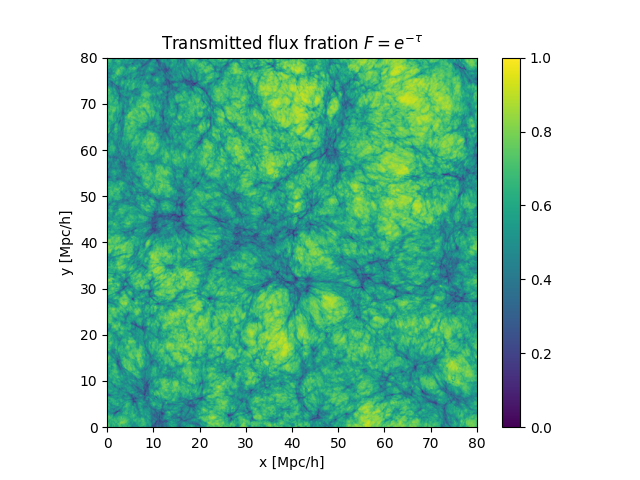
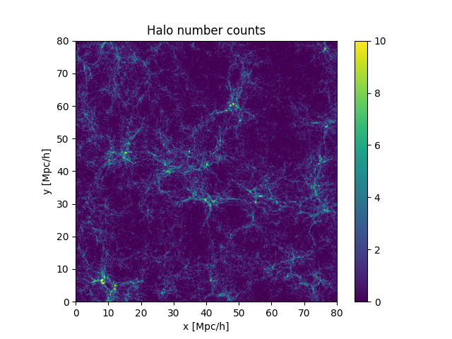
Figure 1: 2D slab of the 3D grids extracted from the $z=2.8$ snapshot in the L80_N1024 simulation, averaged over a depth of $20\ h^{-1}\text{Mpc}$ along the line-of-sight (perpendicular to the plot). The Ly$\alpha$ forest transmitted flux fraction (left) is strongly anti-correlated with the halo number counts (right).

2.1 The Sherwood simulations

The Sherwood simulation suite is a set of large, high-resolution hydrodynamic simulations of the intergalactic medium (IGM) with up to 17.2 billion particles in comoving volumes $10^{3}-160^{3}\,h^{-3}$Mpc³ [54]. The combination of box size and resolution makes them very well-suited for studies of the Ly$\alpha$ forest in the mildly non-linear regime.

All simulations were run using a modified version of the smoothed particle hydrodynamics code P-Gadget3, an updated version of Gadget-2 [56]. The initial conditions were generated at $z=99$ using the N-GenIC code [56] according to an input power spectrum corresponding to a cosmology based on the best-fit flat $\Lambda$CDM model from the first results of the Planck satellite [57], i.e. with $\Omega_{m}=0.308$, $\Omega_{b}=0.0482$, $h=0.678$, $\sigma_{8}=0.829$ and $n_{s}=0.961$.

A homogeneous ionising background is used to calculate photoionization and photo-heating rates assuming the gas is optically thin and in photoionization equilibrium. In this publication we will limit our study to snapshots in the relatively low-redshift range $2<z<3.2$ where BOSS, eBOSS and DESI have measured 3D correlations. As described in [54], Ly$\alpha$ forest measurements at these redshifts are less affected by the reionization model assumed in the simulation relative to measurements at higher redshifts.

As is common in large simulations of the Ly$\alpha$ forest, the computing time is dramatically reduced by removing gas particles at overdensities above $\Delta>1000$ and temperatures below $T<10^{5}K$ and converting them to collisionless particles [21]. This approximation, usually known as Quick-Lya, is valid on the low and intermediate densities that dominate the information in the Ly$\alpha$ forest. However, as discussed in [58, 59], this approximation effectively removes all gas within the virial radius of halos.

In order to properly simulate these high-density regions around massive halos, it would not be enough to keep the gas particles removed by Quick-Lya. We also expect these regions to be affected by different feedback mechanisms not present in the simulations, including the ionizing radiation from quasars themselves. Moreover, we expect the majority of large neutral hydrogen absorbers, including Lyman limit systems and Damped Ly$\alpha$ systems, to come from the vicinity of massive halos; the Sherwood simulations used in this analysis are optically thin, and do not incorporate self-shielding corrections necessary to reproduce the abundances of these systems. In the next sections we will have to keep this in mind when studying the Ly$\alpha$ $\times$ halo cross-correlations on small scales.

The main results discussed in this paper will come from the simulation L160_N2048, where the box size is $L=160\ h^{-1}\text{Mpc}$ and the number of CDM particles and gas particles in the simulation is $N=2048^{3}$. We present some results from the L80_N2048 and the L80_N1024 simulations in appendix A. Even though the Sherwood simulations are the state of the art in terms of hydrodynamical simulations of the Ly$\alpha$ forest, they have not formally converged, and this should be taken into account when interpreting the results.

Ly$\alpha$ datasets typically cover a wide redshift range $2<z<5$. While Ly$\alpha$ BAO results have an effective redshift around $z=2.3$ [9], $P_{\rm 1D}$ analyses have an effective redshift closer to $z=3$ [60]. Most of the results presented in this publication are from a snapshot taken at $z=2.8$, but in appendix B we show results at $z=2.0,2.4,2.8,$ and $3.2$.

2.2 Simulated Ly$\alpha$ forest data

We extract Ly$\alpha$ absorption skewers using the public software fake_spectra which interpolates the gas properties into the requested lines of sight and computes the Ly$\alpha$ optical depth including redshift-space distortions [61].

The IGM around $z=2-4$ is smoothed by gas pressure, suppressing structure on scales smaller than the filtering length $\lambda_{F}\sim 50\ h^{-1}\text{kpc}$ [62]. Unfortunately, memory availability in our post-processing of the simulations limits our analysis to a 3D grid of $(1024)^{2}\times 2048$ cells, with a cell size of $156\ h^{-1}\text{kpc}$ in the transverse direction and $78\ h^{-1}\text{kpc}$ along the line of sight. In appendix A we show that while the measured power spectra are affected by the resolution of these grids, they mostly affect the very high-k modes and do not change the main conclusions presented in this paper.

The left panel of figure 1 shows a 2D slab of the Ly$\alpha$ forest transmitted flux fraction from the snapshot at $z=2.8$ of the smaller L80_N1024 simulation. This is displayed using a grid of $512^{2}\times 1024$ to match the resolution of the main grid used in this section.

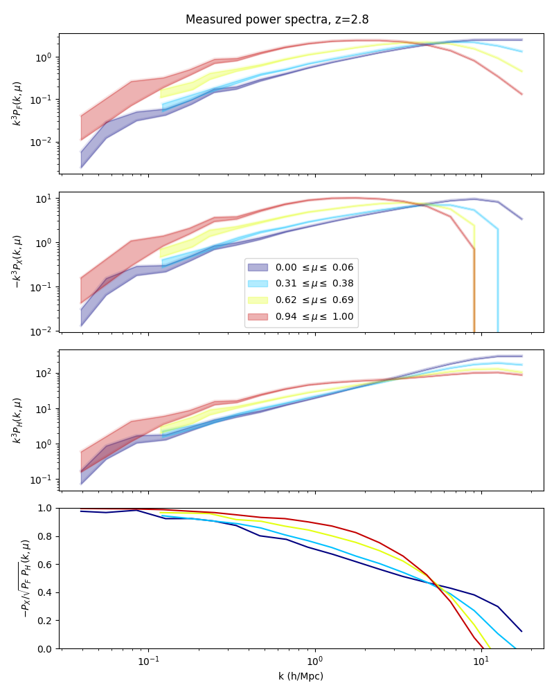
Figure 2: Measured 3D power spectra at $z=2.8$, as functions of wavenumber $k$, for the flux ($P_{F}$), halos ($P_{H}$, shot-noise subtracted) and their cross-correlation ($P_{X}$, multiplied by $-1$). The different colours show the power spectra in 4 of the 16 bins in $\mu$ (orientation with respect to the line of sight, with $\mu=1$ being parallel to the line of sight). The bottom panel shows the correlation coefficient. The sharp cutoff at high wavenumber for the cross-power spectrum arises from a change of sign in the cross-power spectrum.

All Ly$\alpha$ statistics in this paper are computed for fluctuations around a mean transmitted flux fraction, defined as:

$$\delta_{F}(\mathbf{x})\equiv\frac{F(\mathbf{x})}{\bar{F}}-1~{},$$ (2.1)

where $F(\mathbf{x})=e^{-\tau(\mathbf{x})}$ is the transmitted flux fraction, and $\tau(\mathbf{x})$ is Ly$\alpha$ optical depth in redshift space. The upper panel of figure 2 shows the measured power spectrum of the Ly$\alpha$ fluctuations at $z=2.8$ in the larger box (L160_N2048) as a function of wavenumber $k$ and the cosine of the angle between the Fourier mode and the line of sight $\mu$ (modes with $\mu=1$ are parallel to the line of sight).

The power spectra are computed using the average of the square of the norm for all Fourier modes in the box, binned in 16 bins in $\mu$ and 20 log-spaced bins in wavenumber $k$, ranging from the fundamental mode of the box ($k_{0}=2\pi/L=0.039\ h\text{Mpc}^{-1}$) to a maximum wavenumber of $20\ h\text{Mpc}^{-1}$ which is half the Nyquist frequency.

On large scales (small wavenumbers), one can see that the line-of-sight power (red) is boosted by a constant factor with respect to the transverse power (dark blue), as expected in the case of linear bias and linear redshift-space distortions [47]. As discussed later in section 4, non-linearities become important around $k=0.5\ h\text{Mpc}^{-1}$. Non-linear peculiar velocities and thermal broadening suppress the power along the line of sight, before gas pressure smooths the power on all directions around $k=10.0\ h\text{Mpc}^{-1}$.

In order to reduce the cosmic variance in our measurements, we extract Ly$\alpha$ absorption skewers along each of the three axes of the box, using a different component of the 3D velocity vector to include redshift-space distortions [63]. All power spectra discussed in this paper are computed as the average of the power spectra computed along each of the three axes. The errorbars shown in the plots are estimated from the number of Fourier modes entering each band power; they ignore the correlation between measurements along the different axes and the correlation between different Fourier modes within a band power (or across band powers).

The power spectra measurements used in this paper are available online in https://github.com/andreufont/sherwood_p3d.

2.3 Halo grids

The output of the Sherwood simulations includes a halo catalog constructed with a friends of friends algorithm. In order to measure the halo power spectrum and the Ly$\alpha$ $\times$ halo spectrum, we start by discretising this catalog in the same 3D grid that we used for the Ly$\alpha$ skewers. We do this using a nearest-grid-point interpolation. The third panel of figure 2 shows the measured halo power spectrum once the shot-noise, estimated as the inverse of the halo density, has been subtracted.

The second panel of the same figure shows the measured Ly$\alpha$ $\times$ halo spectrum, multiplied by $(-1$) to make it a positive quantity on the largest scales (as seen in figure 1, these fields are anti-correlated). On small, non-linear scales, the cross-power changes sign and becomes positive, causing a sharp feature in this logarithmic plot. It is important to remember that the simulations used the Quick-Lya approximation, replacing gas particles in very high-density regions with collisionless particles, and resulting in a transmission field positively correlated with the halo density on scales comparable to their virial radius.

Finally, the fourth panel of figure 2 shows the correlation coefficient between the two grids, defined as

$$\rho(k,\mu)=\frac{P_{X}(k,\mu)}{\sqrt{P_{F}(k,\mu)P_{H}(k,\mu)}}~{}.$$ (2.2)

On very large scales ($k<0.3\ h\text{Mpc}^{-1}$) the two fields are highly anti-correlated, with $\rho<-0.9$. Even on smaller scales of $k=1\ h\text{Mpc}^{-1}$, the line-of-sight (red) remain 90% anti-correlated, while the anti-correlation has dropped to 70% for the transverse modes (dark blue). This strong anti-correlation motivates the model for the Ly$\alpha$ $\times$ halo spectrum discussed in section 6.

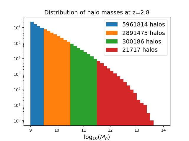
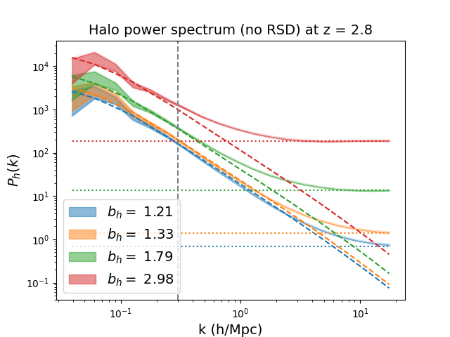
Figure 3: (left) Distribution of halo masses for the halo catalog at $z=2.8$. The different colors identify the four halo mass bins for which we present its power spectrum (right). Note that in this figure we have not added RSDs to the halos and we have not subtracted the Poissonian shot noise (dotted lines). Colored dashed lines show the best-fit one-loop model, as described in section 5.1, with halo biases reported in the legend. The vertical gray dashed line shows the maximum wavenumber ($k=0.3\ h\text{Mpc}^{-1}$) used in the fit.

Our principal motivation in carrying out this study is to improve the modeling of the Ly$\alpha$ $\times$ quasar spectrum; its correlation function analog was recently measured by BOSS and eBOSS [10, 11, 12, 13, 9] and is one of the key measurements expected from DESI. Quasars are highly biased tracers, with typical values of $b_{q}=3.5$ measured at $z\sim 2.5$ [10]. They are typically hosted in dark matter halos larger than $\sim 10^{12}M_{\odot}$ at the relevant redshift range. Unfortunately, as can be seen in figure 3, most of the halos in our simulated box are much smaller — we have only a few thousand halos with a mass similar to those expected to host quasars. Therefore, most plots in this publication use all halos regardless of mass, except in section 6 where we also show the Ly$\alpha$ $\times$ halo power for the highest mass bin.

3 Analysis method

In the next few sections we will present comparisons between different clustering models and the measurements from the simulations presented in figure 2. We will fit models by minimising a pseudo-$\chi^{2}$ function:

$$\chi^{2}(\mathbf{\theta})=\sum_{i}w_{i}\left[P_{i}-P(k_{i},\mu_{i}|\mathbf{\theta})\right]^{2}~{},$$ (3.1)

where $P_{i}$ is the measured power spectrum, $P(k_{i},\mu_{i}|\mathbf{\theta})$ is the theoretical prediction for a set of parameters $\theta$, and $w_{i}$ is the weight given to a particular band power.

We could have weighted each band power using the inverse of its uncertainty, computed from the number ($N^{\rm 3D}_{i}$) of Fourier modes that contribute to each band. However, in this study we combine the power spectrum measured along the three axes of our box, and their modes are not independent. Moreover, as discussed in references [52, 53], the standard fit would be dominated by the high-k data points that have very small errorbars; that would make it difficult to model the large scales comparable to our box size. Following [52, 53], we modify the standard weights by adding a noise floor ($\epsilon$):

$$w_{i}^{-1/2}=P_{i}\left[\frac{1}{\sqrt{N_{i}}}+\epsilon\right]~{}.$$ (3.2)

This noise floor is set by default to $\epsilon=0.05$ as in [53], and it is most relevant for the fits of the flux power spectrum. The shot-noise in the halos already provide a natural noise floor for the halo auto power spectrum and its cross-power spectrum with the Ly$\alpha$ forest. We only include data points with $k<k_{\rm max}$. When fitting the flux power spectrum we use by default $k_{\rm max}=10\ h\text{Mpc}^{-1}$, and we discuss the impact of varying these settings in appendix A. The values of $k_{\rm max}$ used in the auto-correlation of halos and in the Ly$\alpha$ $\times$ halo measurements are discussed in later sections.

4 Modelling the Ly$\alpha$ forest flux power spectrum

The standard linear theory model for Ly$\alpha$ forest flux fluctuations is

$$\delta_{F}=b_{F}\delta+b_{\eta}\eta.$$ (4.1)

Here, $\delta$ is the matter overdensity,

$$\eta=-\frac{1}{aH}\frac{\partial v_{||}}{\partial r_{||}}$$ (4.2)

is the dimensionless gradient of the peculiar velocity $v_{||}$ along the line of sight (represented by comoving coordinate $r_{||})$, $a$ is the scale factor, and $H$ is the Hubble parameter. The fields in equation 4.1 are evaluated in redshift space since the Ly$\alpha$ forest is inherently a redshift-space phenomenon. However, at this order in perturbation theory there is no distinction between real-space coordinate r and redshift-space coordinate s. Bias coefficients $b_{F}$ and $b_{\eta}$ are defined as the partial derivatives of $\delta_{F}$ with respect to $\delta$ and $\eta$, respectively. These coefficients do not have the same interpretation as in the case for galaxies (see [53] for further discussion). The power spectrum associated with equation 4.1 is

$$P_{\textrm{F}}(k,\mu)=b_{F}^{2}(1+\beta_{F}\mu^{2})^{2}P_{L}(k),$$ (4.3)

where $\beta_{F}=b_{\eta}f/b_{F}$ is the RSD parameter with $f$ representing the logarithmic growth rate, $\mu$ is the cosine of the angle between Fourier mode k and the line of sight, and $P_{L}$ is the linear matter power spectrum. We refer to this model as the Kaiser model [47], but it is important to note that the definition of $\beta_{F}$ here includes an extra bias parameter $b_{\eta}$ that is not needed when studying the clustering of point sources.

4.1 Multiplicative corrections to the linear model

Two decades ago, [52] presented a model for the flux power spectrum that was able to fit the 3D power measured in hydro-PM simulations down to very small scales ($k=10\ h\text{Mpc}^{-1}$). It accomplishes this by introducing a multiplicative correction to the linear model, containing 8 free parameters describing non-linearities and the physics of the IGM. That correction term is

$$D_{\rm NL}(k,\mu)=\exp\left\{\left[\frac{k}{k_{\rm{NL}}}\right]^{\alpha_{\rm{NL}}}-\left[\frac{k}{k_{P}}\right]^{\alpha_{P}}-\left[\frac{k_{||}}{k_{V}(k)}\right]^{\alpha_{V}}\right\},$$ (4.4)

with $k_{V}(k)=k_{v0}(1+k/k_{v1})^{a_{v1}}$. The first term in the exponential accounts for isotropic nonlinear growth, the second for isotropic suppression due to pressure, and the third for line-of-sight suppression arising from non-linear peculiar velocities and thermal broadening [52]. The product of equations 4.1 and 4.4 is what we will refer to as the McDonald model.

A similar analysis was carried out the following decade on outputs from GADGET-II simulations [53], and using a modified correction:

$$D_{\rm NL}(k,\mu)=\exp\left\{\Big{[}q_{1}\Delta^{2}(k)+q_{2}\Delta^{4}(k)\Big{]}\left[1-\left(\frac{k}{k_{v}}\right)^{a_{v}}\mu^{b_{v}}\right]-\left(\frac{k}{k_{p}}\right)^{2}\right\},$$ (4.5)

where

$$\Delta^{2}(k)\equiv\frac{k^{3}}{2\pi^{2}}P_{L}(k)$$ (4.6)

is the dimensionless linear matter power spectrum. When comparing this model to the measured flux power spectrum from section 2, we find that the best-fit value for the second order non-linear growth ($q_{2}$) is very close to zero. Therefore we decided to ignore this extra term, reducing the number of free parameters to 5 (compared to the 8 parameters in the McDonald model). We will call the product of equations 4.1 and 4.5 the Arinyo model.

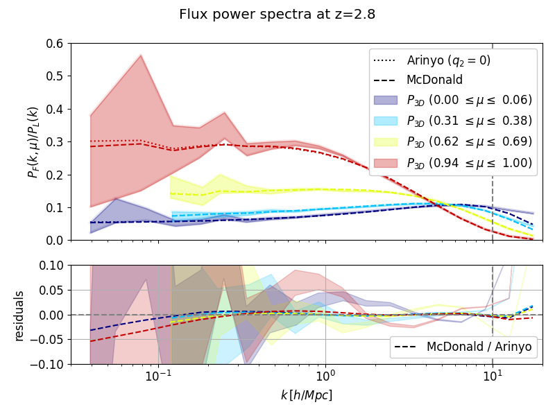
Figure 4: (Top) Model comparison between the Arinyo (with $q_{2}=0$) and McDonald models, and the measured power spectra at $z=2.8$. The 3D power spectra are shown as functions of wavenumber $k$ and orientation $\mu$, divided by the linear power. (Bottom) Residuals with respect to the Arinyo model.

The top panel of figure 4 shows the best-fit predictions for both models compared to the measured 3D power spectra. The 3D power spectra have been divided by the linear power spectrum at the given redshift to highlight the deviations from linear theory on small scales (high-$k$). In the bottom panel, we plot the residuals from the best-fit Arinyo model. Cosmic variance causes large fluctuations on large scales (low-k), but the residuals on intermediate and small scales ($k<10\ h\text{Mpc}^{-1}$) are within 5%.

The ratio of both best-fit models is shown with dashed lines in the bottom panel of figure 4. The best-fit linear bias parameter from the Arinyo model ($b_{F}=-0.234$) is 3% larger than the value from the McDonald model ($b_{F}=-0.227$). As discussed in [53], the modelling of non-linear growth in the McDonald model (an exponential term) extends to much larger scales than the modelling in the Arinyo model. The best-fit values for the RSD parameters are similarly consistent: $\beta_{F}=1.34$ (Arinyo) and $\beta_{F}=1.31$ (McDonald). The minimum values of pseudo-$\chi^{2}$ are also very similar, $\chi^{2}=48.1$ (Arinyo) and $\chi^{2}=48.0$ (McDonald) with 225 data points. Given that the Arinyo model has 3 fewer free parameters, we decide to use that model in the following sections.

4.2 Non-linear growth in the flux power spectrum

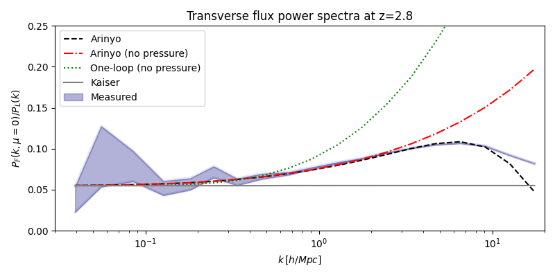
Figure 5: Comparison of different implementations of non-linear growth in the flux power spectrum, for the transverse modes ($\mu=0$). In this plot, only the standard Arinyo model (black dashed line) includes the effect of gas pressure, suppressing the power on scales of $k=10\ h\text{Mpc}^{-1}$.

Recently, [49] presented an analysis of the 1D correlations in the Ly$\alpha$ forest using a model inspired by perturbation theory and effective field theory of large-scale structure. Instead of relying on free parameters to describe the non-linear growth of structure on mildly non-linear scales, the authors used a model (first presented in [48]) that captures non-linearities by using matter and velocity power spectra computed with perturbation theory at one-loop:

$$P_{\rm 3D}(k,\mu)=b^{2}\left[P^{\rm 1-loop}_{\delta\delta}(k)+2\beta\mu^{2}P^{\rm 1-loop}_{\delta\theta}(k)+\beta^{2}\mu^{4}P^{\rm 1-loop}_{\theta\theta}(k)\right]D_{\rm IGM}(k,\mu)~{},$$ (4.7)

where $P^{\rm 1-loop}_{\delta\delta}$, $P^{\rm 1-loop}_{\delta\theta}$, and $P^{\rm 1-loop}_{\theta\theta}$ are the matter-matter, matter-velocity divergence, and velocity divergence-velocity divergence power spectra computed up to 1-loop in perturbation theory (they are equal at tree level). $D_{\rm IGM}$ is a small-scale correction that models gas pressure with an isotropic Gaussian suppression and thermal broadening with another Gaussian suppression along the line of sight. Even though the authors of [49] only proposed this model for analyses of the 1D power spectrum, here we discuss the interesting idea of using perturbation theory at one-loop to model the mildly non-linear regime of the 3D flux power spectrum.

Transverse modes ($\mu=0$) of the flux power spectrum are not affected by redshift-space distortions and offer a cleaner path to study the effect of non-linear growth of structure on the Ly$\alpha$ forest. As can be seen in figure 5, the transverse flux power spectrum at $z=2.8$ (blue band) rises above linear theory around $k=0.3\ h\text{Mpc}^{-1}$ until the effect of gas pressure suppresses the power around $k=7\ h\text{Mpc}^{-1}$. The dashed black line shows the best-fit Arinyo model (again with $q_{2}=0$) from figure 4; the dot-dashed red line shows the same model without the pressure cut-off. The solid gray line further sets $q_{1}=0$, effectively becoming a Kaiser model. Last, the dotted green line shows the prediction from the one-loop model of equation 4.7 without the IGM correction when using the same large scale bias parameters ($b_{F}$,$\beta_{F}$) as the other models.

As we will see in the next sections, these one-loop models (proposed initially by [64] in the context of galaxy clustering) are quite successful in modeling the 3D power spectrum of halos. The Ly$\alpha$ forest, however, is less sensitive to the high-density regions of the box where the flux quickly saturates to $F=0$ and non-linearities in the flux power spectrum grow slower than those in the matter power spectrum. As shown in figure 5, this causes the one-loop model to over-predict the growth of structure in the Ly$\alpha$ forest.

In [49], the impact of non-linearities on the 1D flux power spectrum is captured by adding a counterterm that parameterizes the impact of strong small-scale non-linearities, along the lines of effective field theory (EFT) methods. For the 3D spectrum, the counterterm from [49] is not sufficient, since it describes the influence of non-linear corrections on the integrated 1D spectrum only, by construction. Instead, a more detailed EFT model would be required for the 3D spectrum, along the lines of [65].

Nevertheless, the one-loop model correctly describes the onset of deviations from the linear Kaiser formula, within the regime $k\lesssim 0.5\ h\text{Mpc}^{-1}$ where these corrections are small. This corresponds to the expected range of validity of perturbative methods. Increasing the range of agreement would require to include two-loop terms [48] along with corresponding counterterms [66]. While being limited in $k$ range to weakly non-linear scales, the perturbative treatment has the advantage of being applicable also to non-standard cosmological models and can be evaluated efficiently for a large set of parameters. It is possible to further improve the perturbative description in the BAO range by taking infrared resummation into account [67, 68, 69]. It captures the impact of large-scale flows on the BAO feature in a systematic manner in real and redshift space [70, 71], leading to a broadening of the BAO peak in the correlation function, and a damping of the BAO oscillations in the power spectrum. The IR resummation can easily be implemented in the perturbative model by replacing the linear spectrum that enters the loop computation by a modified input spectrum, obtained by decomposing $P^{\text{lin}}=P^{\text{nw}}+P^{\text{w}}$ into a smooth (non-wiggly) and an oscillating (wiggly) contribution, and multiplying the latter with a particular Gaussian damping factor [70, 71]. While IR resummation is important within the BAO range, it does not change the behaviour of perturbative predictions of the power spectrum in a sizeable way at large wavenumbers $k\gtrsim 0.5\ h\text{Mpc}^{-1}$ shown in figure 5.

5 Modelling the halo power spectrum

5.1 Real-space halo power spectrum

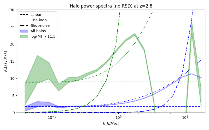
Figure 6: Real space (no RSD) halo power spectrum measured at $z=2.8$ from the whole halo catalog (blue) and from the high-mass bin (green), divided by the linear power spectrum. Dashed (dotted) lines show the best-fit linear (one-loop) model, fitted to $k_{\rm max}=0.3\ h\text{Mpc}^{-1}$. The shot-noise has been subtracted from both the measurement and the models, and it is shown in dot-dashed lines.

The real-space halo power spectrum as a function of halo mass is shown in the right panel of figure 3, together with its best-fit linear model and the shot-noise contribution. In figure 6, we show this again for the largest mass bin (green) and for the total halo catalog (blue), but this time divided by the linear power spectrum of matter fluctuations. Dashed lines show the best-fit linear model, using only large scales ($k_{\rm max}=0.3\ h\text{Mpc}^{-1}$). Dotted lines show the best-fit model when we use a one-loop matter density power spectrum instead. All models and measurements are shown after subtracting the shot-noise, shown as dot-dashed lines for each sample.

Here we model the shot-noise power as the inverse of the halo density. This simple approximation is clearly over-subtracting power in the case of the high-mass halo sample, since the shot-noise subtracted power spectrum becomes negative at $k>3\ h\text{Mpc}^{-1}$. A detailed study of the role of shot-noise in halo clustering can be found in [72].

5.2 Redshift-space halo power spectrum

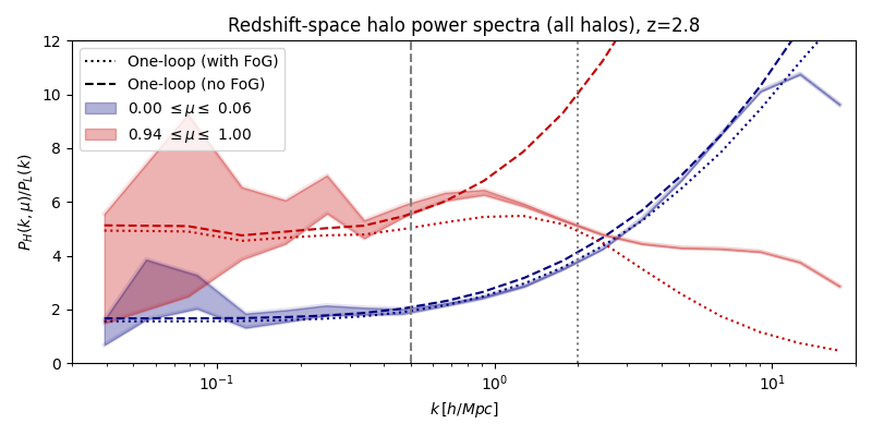
Figure 7: Comparison of the redshift-space halo power spectrum measured at $z=2.8$ along (red) and transverse to (blue) the line of sight. Dotted lines show the best-fit one-loop model (equation 5.2), including a Lorentzian term describing fingers of God (equation 5.3), when fitted to $k_{\rm max}=2\ h\text{Mpc}^{-1}$. Dashed lines show the best-fit one-loop model when using only $k_{\rm max}=0.5\ h\text{Mpc}^{-1}$ and ignoring FoG. The shot-noise has been subtracted from both the measurement and the models.

The ubiquitous model for the clustering of galaxies (or halos) in redshift space was presented by Kaiser [47]:

$$P_{\textrm{h}}(k,\mu)=b_{h}^{2}(1+\beta_{h}\mu^{2})^{2}P_{L}(k).$$ (5.1)

In this equation, $b_{h}$ is the linear halo bias and $\beta_{h}\equiv f/b_{h}$ is the linear RSD parameter for halos. This linear theory description works well on large scales but becomes less accurate past $k\gtrsim 0.5\ h\text{Mpc}^{-1}$ at $z=2.8$. An alternative description of galaxy clustering using non-linear power spectra (equivalent to equation 4.7 without $D_{\rm IGM}$) was presented in [64]:

$$P_{\textrm{h}}(k,\mu)=b_{h}^{2}\Big{[}P^{\rm 1-loop}_{\delta\delta}(k)+2f\mu^{2}P^{\rm 1-loop}_{\delta\theta}(k)+f^{2}\mu^{4}P^{\rm 1-loop}_{\theta\theta}(k)\Big{]}~{}.$$ (5.2)

Non-linear peculiar velocities of halos, often referred to as “Fingers of God” (FoG), suppress the halo power spectrum along the line-of-sight direction. This is often modeled using a Gaussian or Lorentzian distribution as a multiplicative factor to the above equations. In particular, we use a correction of the form

$$D_{\textrm{FoG}}(k,\mu)\equiv\frac{1}{1+(k\mu\sigma_{v})^{2}},$$ (5.3)

where $\sigma_{v}$ is an effective pairwise velocity dispersion parameter [73].

In figure 7 we plot the line-of-sight (red) and transverse (blue) halo power spectrum measured at $z=2.8$, when using all halos in the catalog, and divided by the linear power at that redshift. Dashed lines show the best-fit model when using only the largest scales ($k_{\rm max}=0.5\ h\text{Mpc}^{-1}$) and ignoring FoG, while the dotted lines show the best-fit model including Lorentzian FoG and fitting scales to $k_{\rm max}=2\ h\text{Mpc}^{-1}$. The transverse modes are remarkably well fitted to high $k$, but the line-of sight modes are not well modelled with this simple FoG term. For this reason, in the rest of this paper we do not attempt to model the redshift-space halo power spectrum, and we obtain the large-scale halo bias from the real-space halo power spectrum (figure 6).

6 Modelling the Ly$\alpha$ forest-halo cross-power spectrum

In figure 8 we show the same Ly$\alpha$ $\times$ halo power spectra that is also shown in figure 2, but this time divided by the linear power spectrum of matter fluctuations at the same redshift. In this section we discuss models to describe the non-linearities in this measurement.

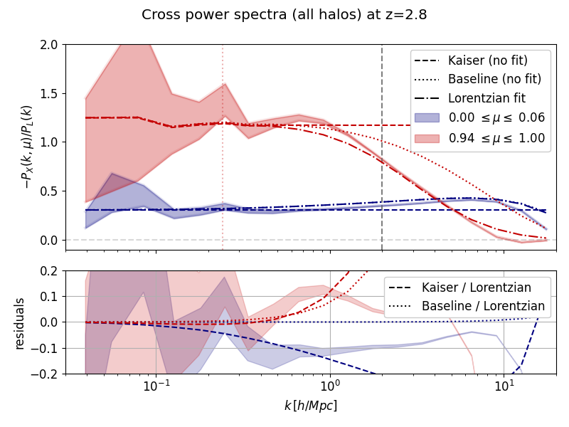
Figure 8: (Top) Measured Ly$\alpha$ $\times$ halo cross-power spectra when using all halos in the snapshot (shaded regions), divided by the linear power spectrum, as a function of wavenumber $k$ and orientation with respect to the line of sight $\mu$. Dashed and dotted lines show the predictions based on the Kaiser model and on equation 6.2 respectively, both without any free parameter. Dot-dashed lines show the best-fit model after adding an extra parameter $\sigma_{v}$ to account for fingers of God with a Lorentzian term, using wavenumbers smaller than $k_{\rm max}=2\ h\text{Mpc}^{-1}$, marked with a vertical dashed gray line. Vertical color dotted lines show the scales where quasar redshift errors of $500~{}{\rm km~{}s^{-1}}$ would suppress half of the power. (Bottom) Residuals with respect to the best-fit Lorentzian model.

6.1 Linear model

Given that the Kaiser model can describe the large-scale clustering of both tracers (halos and Ly$\alpha$ forest), and that these are strongly anti-correlated on large scales (see bottom panel of figure 2), one expects that the Kaiser model should also describe the Ly$\alpha$ $\times$ halo cross-correlation on linear scales. This model can be computed as the geometric mean of the Kaiser models for both tracers, equations 4.3 and 5.1:

$$P_{\textrm{Fh}}(k,\mu)=\sqrt{P_{\textrm{F}}(k,\mu)~{}P_{\textrm{h}}(k,\mu)}=b_{h}(1+\beta_{h}\mu^{2})~{}b_{F}(1+\beta_{F}\mu^{2})~{}P_{L}(k)~{}.$$ (6.1)

Indeed, figure 8 shows that the large-scale cross-power is proportional to the linear power spectrum, with a boost in line-of-sight modes caused by linear RSDs.

This linear theory model was used in the first measurement of the Ly$\alpha$-quasar cross correlation in BOSS at $z=2.3$ over scales $r>15\ h^{-1}\text{Mpc}$ [10]. The authors also included a multiplicative correction, similar to equation 5.3, to model the suppression of power caused by quasar redshift errors and non-linear quasar velocities. They obtained values for the velocity dispersion of the order of $500\,{\rm km~{}s^{-1}}$, and argued that these were dominated by quasar redshift errors.

6.2 Building nonlinear models

BAO measurements using the cross-correlation of quasars and the Ly$\alpha$ forest from BOSS and eBOSS [11, 12, 8, 13, 9] used a modified version of equation 6.1. They replaced $P_{L}(k)$ by a quasi-linear power spectrum that decoupled the BAO peak from the smooth component in order to model the non-linear broadening of the BAO peak [74] (see also discussion at the end of section 4). However, given the limited box size of our simulations, we do not attempt to model this non-linear broadening of the BAO wiggles, and we will focus here on the deviations from linear theory on small scales.

In order to build our first non-linear model for the Ly$\alpha$ $\times$ halo correlations, we use again the geometrical mean of the two power spectra. This time, however, we use the Arinyo model to describe the flux component:

$$P_{\textrm{Fh}}(k,\mu)=b_{h}(1+\beta_{h}\mu^{2})~{}b_{F}(1+\beta_{F}\mu^{2})~{}P_{L}(k)~{}\sqrt{D_{\rm NL}(k,\mu)}~{},$$ (6.2)

where $D_{\rm NL}(k,\mu)$ is the small-scales correction described in equation 4.5. We will refer to this equation as the baseline model for the Ly$\alpha$ $\times$ halo cross-correlation.

Instead of fitting this model to the measured cross-correlation, we start by making predictions when using the best-fit values measured from the Ly$\alpha$ forest auto-correlation in section 4, and the halo bias measured from the halo auto-correlation in section 5. Because of the difficulties in modelling RSDs in the halo power spectrum, we use instead the halo bias measured from the real space halo power spectrum (see figure 6). The dotted lines in figure 8 show the predicted cross-correlation using equation 6.2. Unfortunately, this simple model (without any free parameter) does not seem to perform any better than the Kaiser model, and it overpredicts the signal in the transverse direction (blue lines).

In order to improve the model for the line-of-sight signal (in red), we also add a fit that includes an extra term to model Fingers-of-God (FoG) in the halos:

$$P_{\textrm{Fh}}(k,\mu)=b_{h}(1+\beta_{h}\mu^{2})~{}b_{F}(1+\beta_{F}\mu^{2})~{}P_{L}(k)~{}\sqrt{D_{\rm NL}(k,\mu)~{}D_{\rm FoG}(k,\mu)}~{},$$ (6.3)

where $D_{\rm FoG}(k,\mu)$ is the Lorentzian function from equation 5.3. The dot-dashed lines in the top panel of figure 8 show the best-fit model when fitting $\sigma_{v}$ using wavenumbers smaller than $k_{\rm max}=2\ h\text{Mpc}^{-1}$ (gray dashed vertical line).

The bottom panel of figure 8 shows the residuals for the Ly$\alpha$ $\times$ halo power when using the Baseline model (no free parameters), as well as the ratio of the different models. The simple Kaiser model of equation 6.1 properly describes the measured correlations up to $k=1\ h\text{Mpc}^{-1}$, with an accuracy better than 5%. The other models, however, seem to overpredict the clustering of the transverse modes (blue lines).

It is important to keep in mind that measurements of the cross-correlation of quasars and the Ly$\alpha$ forest are affected by quasar redshift errors. Assuming a Gaussian suppression with $\sigma_{v}=500~{}{\rm km~{}s^{-1}}$, typical of quasar surveys at $z>2$ [9], we compute the wavenumber where half of the power would be suppressed. These are shown as vertical colored dotted lines, as a function of $\mu$. Disagreements on scales much smaller than these are not necessarily relevant, since they will be highly suppressed by quasar redshift errors when analysing real data.

6.3 Dependency on halo mass

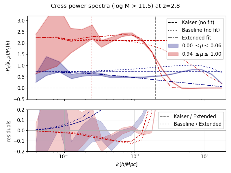
Figure 9: Same as figure 8, but limited to the most massive halos. Dashed and dotted lines show the predictions based on the Kaiser model and on equation 6.2 respectively, both without any free parameter. Dot-dashed lines show the best-fit model after adding the three extra parameters ($\alpha$, $\gamma$, $\nu$) in our extended model. The fit uses wavenumbers smaller than $k_{\rm max}=2\ h\text{Mpc}^{-1}$, marked with a vertical dashed gray line.

As discussed at the end of section 2.3, most of the halos in our simulation are significantly smaller than those expected to host quasars. Therefore, the measurements of the cross-correlation presented above might not be representative of the cross-correlation with quasars. However, the green lines in figure 6 show that the clustering of the most massive halos in the simulation is strongly affected by shot-noise on scales of $k>0.5\ h\text{Mpc}^{-1}$.

In figure 9 we show the Ly$\alpha$ $\times$ halo cross-power when looking at halos in the largest mass bin. We can see that the baseline prediction of equation 6.2 (dotted lines) overpredicts the clustering already on fairly linear scales ($k<0.3\ h\text{Mpc}^{-1}$). These deviations are also present at $\mu=0$ (blue lines), and cannot be related to non-linear RSDs or FoG. If one used the one-loop power spectrum instead of the linear one in equation 6.2, the deviations would be even larger.

As can be seen in the left panel of figure 12, massive halos are less (anti) correlated with the Ly$\alpha$ forest, particularly for transverse modes where the correlation coefficient is only $\rho=-0.7$ at $k=0.3\ h\text{Mpc}^{-1}$, and $\rho=-0.5$ at $k=0.5\ h\text{Mpc}^{-1}$. Therefore, instead of trying to improve the non-linear modelling, we developed a more complex (Extended) model that adds to equation 6.2 an ad-hoc multiplicative correction to capture the anisotropic decorrelation of both fields:

$$D_{\textrm{M}}(k,\mu)\equiv\exp\Big{[}(\alpha+\gamma\mu^{2})\Delta^{2}(k)-(k\mu\nu)^{4}\Big{]},$$ (6.4)

where $\alpha$, $\gamma$, and $\nu$ are free parameters, and $\Delta^{2}(k)$ is the dimensionless linear power as described in equation 4.6. The dot-dashed lines in figure 9 show the best-fit predictions for this extended model, and the bottom panel shows the residuals with respect to this fit. In this case the residuals are smaller than 10% up to scales of $k=1\ h\text{Mpc}^{-1}$.

It is important to remember, however, that the measurement on these scales is probably impacted by the Quick-Lya approximation used in the simulations. As shown in [58], the impact of the approximation is more important for massive halos with large virial radius.

7 Discussion

7.1 Prediction of 1D correlations from 3D models

In section 4 we have shown that the Arinyo model can successfully describe the full shape of 3D correlations down to small scales. Integrating the 3D model with equation 7.1, one can also obtain a prediction for the 1D correlations:

$$P_{\rm 1D}(k_{\parallel})=\frac{1}{\pi}\int_{0}^{\infty}dk_{\perp}~{}k_{\perp}~{}P_{\rm 3D}(k_{\parallel},k_{\perp})~{},$$ (7.1)

where $k_{\parallel}=k\mu$, and $k_{\perp}=k\sqrt{1-\mu^{2}}$. The 1D power spectrum measured at a given line-of-sight wavenumber $k_{\parallel}$ is therefore sensitive to the 3D power spectrum over all transverse modes $k_{\perp}$.

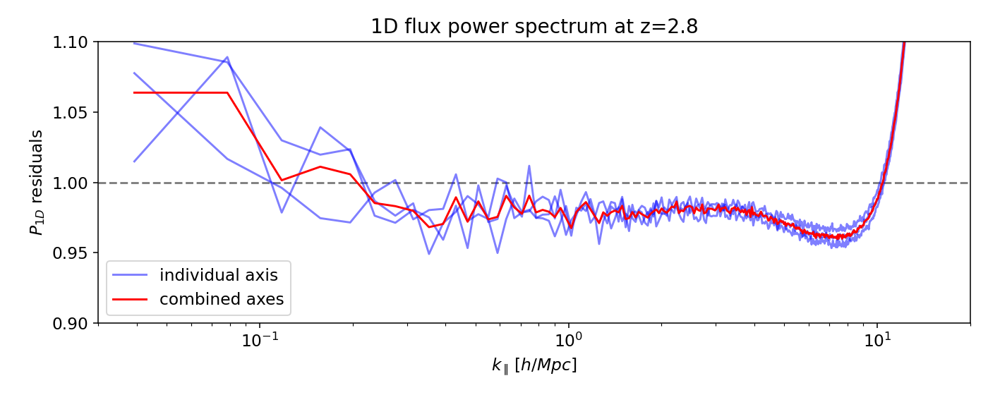
Figure 10: One-dimensional flux power spectrum measured along each simulation axis (blue), and its mean (red), divided by the prediction from the best-fit Arinyo model from section 4.

The blue lines in figure 10 show the P1D measurement from Ly$\alpha$ forest skewers along the three different simulation axes, divided by the prediction from the best-fit Arinyo model in section 4. The red line is the mean of the three blue lines, and is our best measurement of 1D correlations from the simulation. The $6\%$ differences on the largest scales might be explained by cosmic variance, and the deviations on smaller scales are less than $2\%$ on scales relevant for BOSS, eBOSS or DESI analyses ($k_{\parallel}<4\ h\text{Mpc}^{-1}$).

7.2 Impact on BAO studies

So far, we have presented measurements and models of power spectra, correlations in Fourier space. However, BAO studies using the Ly$\alpha$ forest to date have used the correlation function. In figure 11 we show the model correlations in configuration space for the flux auto-correlation (top panels), and for the Ly$\alpha$ $\times$ halo cross-correlation when using the most massive halos (bottom panels). Solid color lines show the correlations for the main Arinyo model (top panels), for different orientations with respect to the line of sight $\mu$, and for the extended cross-correlation model from section 6.3 (bottom panels). Black dotted lines show the equivalent correlations for the corresponding Kaiser model, where we have set $D_{NL}=1$ and used the same values of the linear bias parameters.

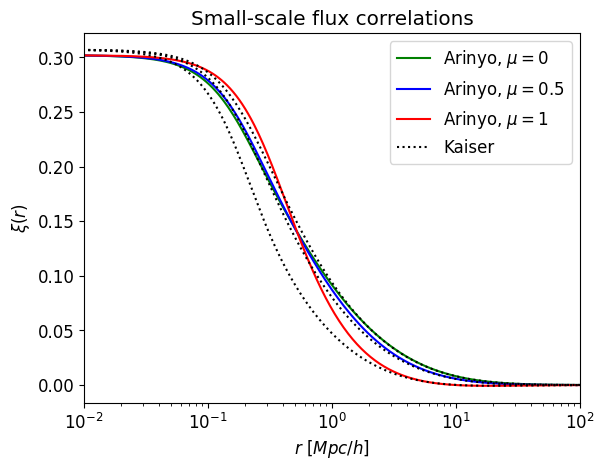
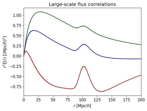
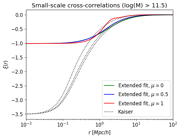
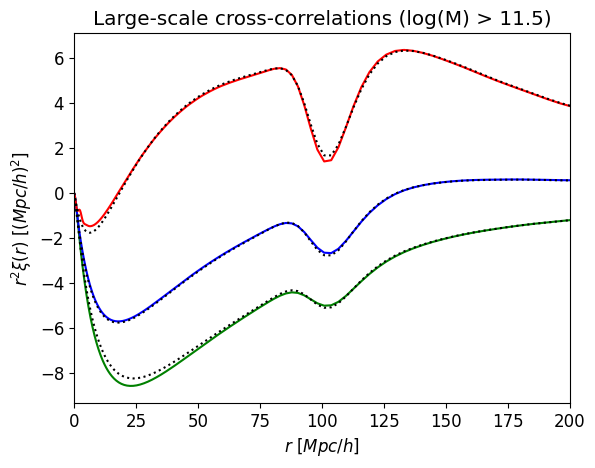
Figure 11: Correlation functions corresponding to the best-fit models obtained in previous sections, for different orientations with respect to the line of sight $\mu$. Solid color lines show the best-fit Arinyo model for the Ly$\alpha$ forest auto-correlation shown in figure 4 (top panels); the best-fit extended model for the Ly$\alpha$ $\times$ halo cross-correlation when using only halos in the largest mass bin, as in figure 9 (bottom panels). Black dotted lines show the equivalent correlations for the corresponding Kaiser model, using the same values of the linear bias parameters. Left panels show correlations on small separations, while the right panels show large-scale correlations multiplied by $r^{2}$ to highlight the BAO feature.

In order to compute these model correlations, we have computed the predicted multipoles of the power spectra up to the 10th order in the Legrendre decomposition, and we have computed their inverse Fourier transform using the FFTLog formalism as implemented in mcfit .

The differences between the models are clear when looking on small scales (left panels), but on the large scales used in BAO analyses (right panels) the differences are significantly smaller, especially for the flux auto-correlation. Recently, [14] has proposed using the anisotropy of these correlations to constraint cosmology by performing an Alcock-Paczińsky test. Figure 11 shows that deviations from linear theory should be relatively small if one considers only separations larger than $30\ h^{-1}\text{Mpc}$ or so.

7.3 Problems modelling the cross-correlation for massive halos

As discussed in section 2.3, the limited box size of the simulations results in relatively few halos with masses comparable to those hosting quasars. More importantly, as discussed in section 2.1, the Quick-Lya approximation used in this and many other simulations of the Ly$\alpha$ forest artificially removes gas from the high-density regions and biases the measurements of the Ly$\alpha$ $\times$ halo correlation on small scales. Besides these issues with the measurements, in this section we discuss three other problems that we encounter when modelling the Ly$\alpha$ $\times$ halo cross-correlation.

First, as discussed in appendix B of [75], the cross-correlation of halos with the Ly$\alpha$ forest can be computed as the mean value of the Ly$\alpha$ fluctuations at a given separation from a halo:

$$\xi_{X}(r)=\langle\delta_{F}\rangle_{r}~{},$$ (7.2)

where the expected value is computed using only pixels at a separation $r$. In the absence of instrumental noise, the value of flux can not be negative. This implies that the cross-correlation always has to satisfy $\xi_{X}(r)\geq-1$. However, our power spectrum models do not know about this natural threshold. As can be seen in the bottom-left panel of figure 11, it seems that our extended model asymptotically reaches $\xi_{X}=-1$. However, we have tested that small variations in the model result in non-physical correlations with $\xi_{X}(r)<-1$.

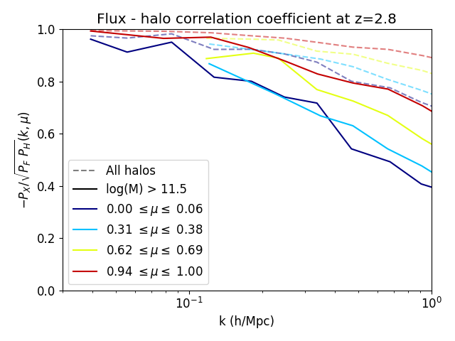
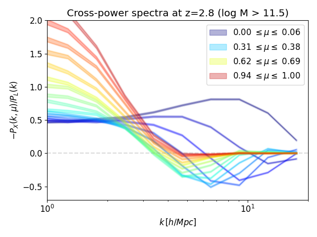
Figure 12: Left: Correlation coefficient between halos and the Ly$\alpha$ forest, for the most massive halos (solid lines) and for the complete catalog (dashed). Right: Cross-correlation of the most massive halos on the smallest scales, divided by the linear power spectrum.

Second, the models discussed in section 6 are motivated by the assumption that the Ly$\alpha$ forest field and the halo density are strongly (anti-) correlated, and try to build a model from the geometrical mean of auto-correlation models. However, in the left panel of figure 12 we compare the correlation coefficient when using all halos (dashed lines, also seen in figure 2) and when using only the most massive halos (solid lines). For the massive halos, half of the anti-correlation has already been lost on scales of $k=0.5\ h\text{Mpc}^{-1}$. The ad-hoc correction from equation 6.4 can capture this by fitting negative values for $\alpha$, but it is difficult to propose physically-motivated models when the fields become increasingly uncorrelated.

Finally, our models assume that the cross-power spectrum is negative on all scales. However, the right panel of figure 12 clearly shows that the cross-power for the most massive halos changes sign around $k=3\ h\text{Mpc}^{-1}$, except for the most transverse modes (in dark blue). This might be a consequence of the Quick-Lya approximation used in the simulations, and it would be interesting to carry out an equivalent study of these small-scale correlations in configuration space.

8 Conclusions

We have presented the most accurate measurement of the 3D power spectrum of fluctuations in the Ly$\alpha$ forest to date, using outputs from the Sherwood suite of hydrodynamic simulations . These simulations are considerably larger (20 times more particles) than those used in the current state-of-the-art measurements of [53]. We have also presented, for the first time, a measurement of the Ly$\alpha$ $\times$ halo 3D cross-power spectrum. The Ly$\alpha$ forest and the halo catalog are strongly anti-correlated on all scales relevant for BAO analyses ($\rho<-0.9$ at $k<0.3\ h\text{Mpc}^{-1}$). The most massive halos, however, are less anti-correlated (left panel of figure 12). We have made these measurements public to encourage other teams to work on the modelling of these correlations.

We have confirmed that the non-linear models of [52] and [53] are able to describe the 3D flux power spectrum down to small scales, and that the second-order non-linear growth parameter ($q_{2}$) in [53] is not required to obtain a good fit. In figures 4 and 10 we show that the Arinyo model can predict at the same time 1D and 3D correlations, with 3D residuals smaller than 5% on scales smaller than $k<10\ h\text{Mpc}^{-1}$, and 1D residuals smaller than 2% for $k<4\ h\text{Mpc}^{-1}$. This opens the possibility of joint fits of 1D and 3D correlations observed by BOSS and eBOSS, and the possibility of building 1D emulators based on 3D models. The non-linearities in the Ly$\alpha$ forest power spectrum are smaller than those in the matter power spectrum (see figure 5). Dense regions in the simulation quickly saturate the transmitted flux fraction to $F=0$, acting as a natural shield that protects the Ly$\alpha$ forest from the details of non-linear growth.

The bottom panel of figure 8 shows that the Kaiser model describes the Ly$\alpha$ $\times$ halo power spectrum with residuals smaller than 5% even on scales as small as $k=1\ h\text{Mpc}^{-1}$, when using all halos in the simulation. However, it does not describe well the correlation with the most massive halos, representative of quasars. In equation 6.4 we present an ad-hoc multiplicative correction to the model that can improve the fit considerably, with residuals smaller than 10% up to $k<1\ h\text{Mpc}^{-1}$.

Even though the Sherwood suite is the state of the art in terms of simulations of the Ly$\alpha$ forest, in appendix A we show that the measurements presented here are still affected by their limited box size and resolution. Uncertainties in the cosmological model assumed in the simulation, as well as in the assumed thermal and ionization history, could also modify significantly the measured power spectra. For this reason we do not focus on the actual best-fit parameter values that we obtain when analysing this particular simulation; as we show in appendix A, both the large scale bias and the pressure terms are affected by the limitations of the simulations.

In section 7 we list a couple of fundamental issues with our approach to model the Ly$\alpha$ $\times$ halo cross-correlation. By definition, the cross-correlation function cannot be more negative than $\xi=-1$ (corresponding to $F=0$ or $\delta_{F}=-1$), but our Fourier-space models are not aware of this. A second limitation of our models is that they are not allowed to change sign, while the measured Ly$\alpha$ $\times$ halo cross-power seems to change sign around $k=3\ h\text{Mpc}^{-1}$ as shown in the right panel of figure 12. We caution the reader that the measurement itself can be corrupted in these small scales. The Quick-Lya approximation used in the simulations artificially removes gas from the vicinity of the dark matter halos.

Finally, in figure 11 we show that on scales relevant for BAO analyses, the best-fit non-linear models predict small deviations from linear theory. This is particularly true for the Ly$\alpha$ forest auto-correlation, while larger deviations in the cross-correlation with the most massive halos appear on scales below $r=30\ h^{-1}\text{Mpc}$ for the most transverse separations.

This investigation is timely since the Dark Energy Spectroscopic Instrument (DESI [76]) started its five-year program in May 2021, and it will soon provide the largest Ly$\alpha$ forest dataset to date. While the main goal of the DESI Ly$\alpha$ dataset is to measure BAO, this study is a step towards cosmological analyses using the full shape of the 3D correlations.

Appendix A Alternative analyses of flux power spectrum

A.1 Convergence of simulation boxes

Most measurements discussed in the main text use the largest simulation L160_N2048, with box size $L=160\ h^{-1}\text{Mpc}$ and $N=2048^{3}$ CDM and gas particles. In order to study the impact of box size, in the left panel of figure 13 we compare the measurement from this box with the measurement from a simulation that has the same particle resolution, but a smaller box size (L80_N1024). Sample variance due to the limited box sizes makes it difficult to compare the large-scale measurement, but one can see small differences extending to all scales. Note, however, that this ratio is affected by interpolation artifacts, since the values of wavenumbers $k$ in the two measurements do not match.

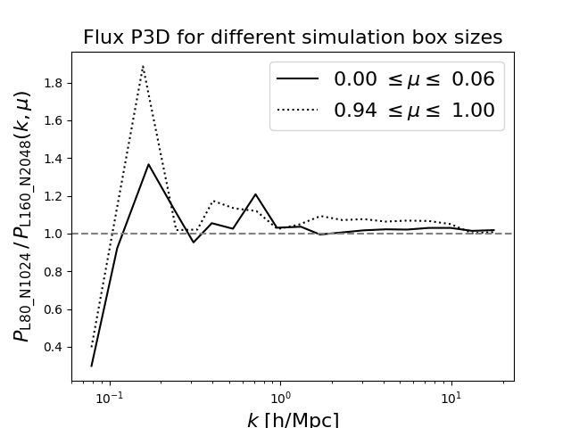
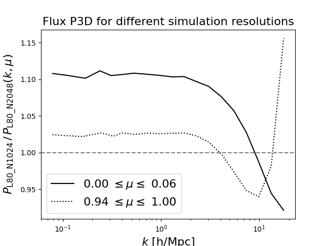
Figure 13: Left: Ratio of Ly$\alpha$ forest power spectrum in two simulations with the same particle resolution, but different box size. The differences at low-k are probably explained by cosmic variance. The computation of the ratio on all scales is affected by interpolation artifacts, since the values of wavenumbers $k$ in the two measurements do not match. Right: Ratio of Ly$\alpha$ forest power spectrum in two simulations with the same box size, but different particle resolution.

In the right panel of figure 13 we study the impact of particle resolution, using two simulations with $L=80\ h^{-1}\text{Mpc}$, but different number of particles. The simulation L80_N1024 has the same particle resolution as the box used in the main text, while the simulation L80_N2048 has 8 times more particles in the same volume. On large scales, particle resolution impacts the value of the large scale bias and redshift space distortion parameter, at the order of a few percent. On small scales, the gas in the simulation with lower particle resolution seems to have a stronger pressure smoothing.

A.2 Convergence of grids

Memory restrictions in the post-processing of the simulations limit our analysis to a 3D grid of $(1024)^{2}\times 2048$ cells, with a cell size of $0.156\ h^{-1}\text{Mpc}$ in the transverse direction and $0.078\ h^{-1}\text{Mpc}$ along the line of sight. Here we study the impact of this pixelisation in the flux power, using the L80_N1024 simulation, with a smaller box but the same resolution as our largest simulation.

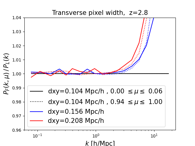
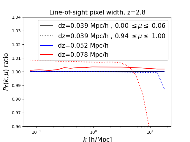
Figure 14: Measured flux power spectrum at $z=2.8$, from different settings of the 3D grid of the L80_N1024 box. Left: impact of transverse pixel size in the flux grid, for the default value of line-of-sight pixel width of $dz=0.078\ h^{-1}\text{Mpc}$. The default value of $dxy=0.156\ h^{-1}\text{Mpc}$ is enough to capture the effect of pressure smoothing, but the results are not fully converged. Right: impact of line-of-sight pixelisation in the grid. The default value of $dz=0.078\ h^{-1}\text{Mpc}$ (the best we can use on our larger box) does not resolve the line-of-sight structure, and this results in a percent difference in the large scale power, and a 4 % difference on the smallest scale used in the analysis.

In figure 14 we compare the 3D flux power from our default simulation box, when varying the resolution of the 3D grid. In the left panel we vary the transverse resolution of the grid, and show that even the default setting (blue line) is not quite converged, with 4% differences on the smallest scales used in the fits. In the right panel we vary instead the line-of-sight pixelisation, and show that the default pixelisation (red lines) caused a biased measurement of the large-scale power of order 1%, and a bias of order 4% on the smallest scales used in the fits.

A.3 Alternative fit configurations

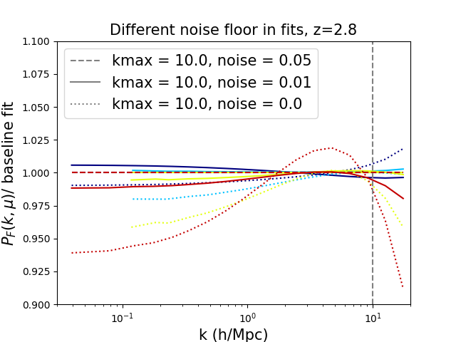
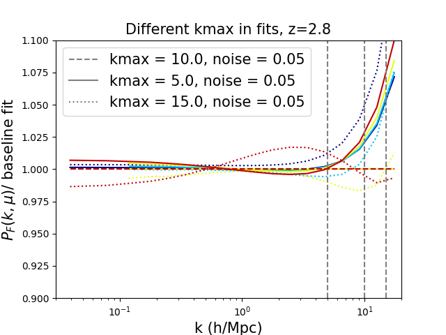
Figure 15: Ratio of best-fit models for the flux power spectra, for different fitting configurations on the best-fit Arinyo model. Left: effect of varying the noise floor $\epsilon$ in equation 3.2. Right: effect of varying the maximum wavenumber $k_{\rm max}$ included in the fit.

As described in section 3, the default analysis of the flux power spectrum minimises a pseudo-$\chi^{2}$, defined in equation 3.1, that weights the different band powers based on the number of Fourier modes that contribute to a particular bin. In order to down-weight high-k modes, that would otherwise dominate the fit, we follow [52, 53] and modify the weights by adding a noise floor ($\epsilon$) (equation 3.2). The left panel of figure 15 shows the impact of $\epsilon$ on the best-fit Arinyo model. While the default analyses uses the same value of $\epsilon=0.05$ used in [53], a noise floor five times smaller give almost indistinguishable results (solid lines). Ignoring the noise floor completely (dotted lines) have a noticable impact on the best-fit large-scale biases.

In the right panel of figure 15 we study the impact of varying the maximum wavenumber $k_{\rm max}$ used in the fits. Decreasing (solid) or increasing (dotted) the default value of $k_{\rm max}=10\ h\text{Mpc}^{-1}$ have only minor effects on the best fit, mostly limited to the modelling of pressure on the smallest scales.

Appendix B Results at different redshifts

Most of the analyses presented in this paper use the snapshot at $z=2.8$. However, the Ly$\alpha$ forest data usually spans a wide range of redshift, and in this appendix we reproduce some of the key results at different redshifts. In order to reduce the computational requirements of this comparison, we use outputs from the small box simulation L80_N1024 ($80\ h^{-1}\text{Mpc}$, $1024^{3}$ particles) and the same grid resolution than the main analysis. This is justified by the convergence tests presented in appendix A.

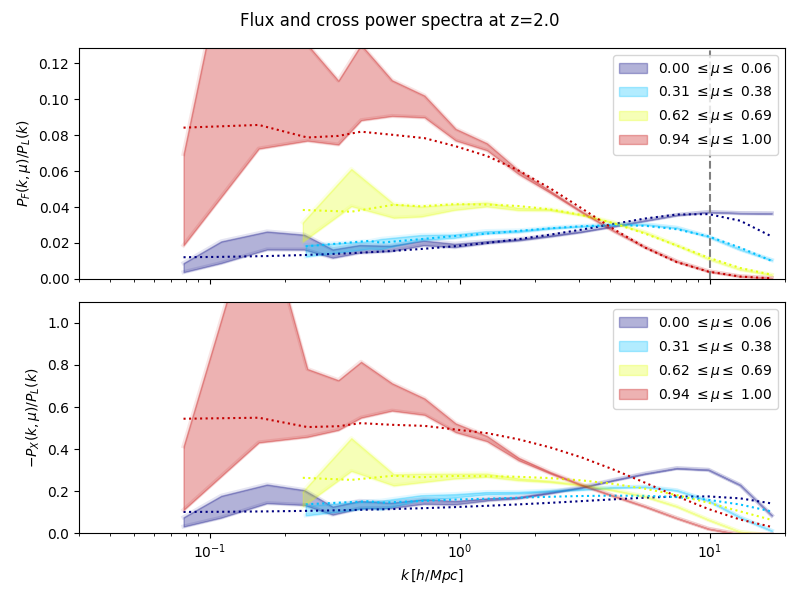
Figure 16: Measurements and models of power spectra at $z=2.0$, using the L80_N1024 simulation with the same resolution than the one used in the main test. Top: flux power spectrum and best-fit Arinyo model, similar to figure 4. Bottom: cross power-spectrum and baseline model (without free paramters) for the total halo catalog, similar to LABEL:fig:cross.

In figures 16, 17, 18 and 19 we redo the analysis of the flux power (top panels) and Ly$\alpha$ $\times$ halo power (bottom panels) at redshifts $z=2.0$, $2.4$, $2.8$ and $3.2$. At all redshifts the flux power is well described by the Arinyo model, while the baseline model for the Ly$\alpha$ $\times$ halo cross-correlation (without free parameters) is only a good description on relatively large scales.

Figure 17: Same as figure 16, but at $z=2.4$.

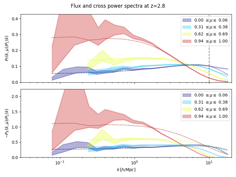
Figure 18: Same as figure 16, but at $z=2.8$.

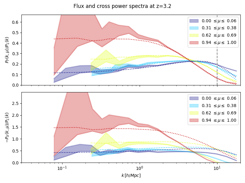
Figure 19: Same as figure 16, but at $z=3.2$.

References

- [1] K. S. Dawson, D. J. Schlegel, C. P. Ahn, S. F. Anderson, É. Aubourg, S. Bailey et al., The Baryon Oscillation Spectroscopic Survey of SDSS-III, AJ 145 (2013) 10 [1208.0022].
- [2] K. S. Dawson, J.-P. Kneib, W. J. Percival, S. Alam, F. D. Albareti, S. F. Anderson et al., The SDSS-IV Extended Baryon Oscillation Spectroscopic Survey: Overview and Early Data, AJ 151 (2016) 44 [1508.04473].
- [3] A. Slosar, A. Font-Ribera, M. M. Pieri, J. Rich, J.-M. Le Goff, É. Aubourg et al., The Lyman- forest in three dimensions: measurements of large scale flux correlations from BOSS 1st-year data, JCAP 2011 (2011) 001 [1104.5244].
- [4] N. G. Busca, T. Delubac, J. Rich, S. Bailey, A. Font-Ribera, D. Kirkby et al., Baryon acoustic oscillations in the Ly forest of BOSS quasars, Astron. Astrophys. 552 (2013) A96 [1211.2616].
- [5] A. Slosar, V. Iršič, D. Kirkby, S. Bailey, N. G. Busca, T. Delubac et al., Measurement of baryon acoustic oscillations in the Lyman- forest fluctuations in BOSS data release 9, JCAP 2013 (2013) 026 [1301.3459].
- [6] T. Delubac, J. E. Bautista, N. G. Busca, J. Rich, D. Kirkby, S. Bailey et al., Baryon acoustic oscillations in the Ly forest of BOSS DR11 quasars, Astron. Astrophys. 574 (2015) A59 [1404.1801].
- [7] J. E. Bautista, N. G. Busca, J. Guy, J. Rich, M. Blomqvist, H. du Mas des Bourboux et al., Measurement of baryon acoustic oscillation correlations at z = 2.3 with SDSS DR12 Ly-Forests, Astron. Astrophys. 603 (2017) A12 [1702.00176].
- [8] V. de Sainte Agathe, C. Balland, H. du Mas des Bourboux, N. G. Busca, M. Blomqvist, J. Guy et al., Baryon acoustic oscillations at z = 2.34 from the correlations of Ly absorption in eBOSS DR14, Astron. Astrophys. 629 (2019) A85 [1904.03400].
- [9] H. du Mas des Bourboux, J. Rich, A. Font-Ribera, V. de Sainte Agathe, J. Farr, T. Etourneau et al., The Completed SDSS-IV Extended Baryon Oscillation Spectroscopic Survey: Baryon Acoustic Oscillations with Ly Forests, ApJ 901 (2020) 153 [2007.08995].
- [10] A. Font-Ribera, E. Arnau, J. Miralda-Escudé, E. Rollinde, J. Brinkmann, J. R. Brownstein et al., The large-scale quasar-Lyman forest cross-correlation from BOSS, JCAP 2013 (2013) 018 [1303.1937].
- [11] A. Font-Ribera, D. Kirkby, N. Busca, J. Miralda-Escudé, N. P. Ross, A. Slosar et al., Quasar-Lyman forest cross-correlation from BOSS DR11: Baryon Acoustic Oscillations, JCAP 2014 (2014) 027 [1311.1767].
- [12] H. du Mas des Bourboux, J.-M. Le Goff, M. Blomqvist, N. G. Busca, J. Guy, J. Rich et al., Baryon acoustic oscillations from the complete SDSS-III Ly-quasar cross-correlation function at z = 2.4, Astron. Astrophys. 608 (2017) A130 [1708.02225].
- [13] M. Blomqvist, H. du Mas des Bourboux, N. G. Busca, V. de Sainte Agathe, J. Rich, C. Balland et al., Baryon acoustic oscillations from the cross-correlation of Ly absorption and quasars in eBOSS DR14, Astron. Astrophys. 629 (2019) A86 [1904.03430].
- [14] A. Cuceu, A. Font-Ribera, B. Joachimi and S. Nadathur, Cosmology beyond BAO from the 3D distribution of the Lyman- forest, Mon. Not. Roy. Astron. Soc. 506 (2021) 5439 [2103.14075].
- [15] C. Alcock and B. Paczynski, An evolution free test for non-zero cosmological constant, Nature 281 (1979) 358.
- [16] R. A. C. Croft, D. H. Weinberg, N. Katz and L. Hernquist, Recovery of the Power Spectrum of Mass Fluctuations from Observations of the Ly Forest, ApJ 495 (1998) 44 [astro-ph/9708018].
- [17] R. A. C. Croft, D. H. Weinberg, M. Pettini, L. Hernquist and N. Katz, The Power Spectrum of Mass Fluctuations Measured from the Ly Forest at Redshift z = 2.5, ApJ 520 (1999) 1 [astro-ph/9809401].
- [18] P. McDonald, J. Miralda-Escudé, M. Rauch, W. L. W. Sargent, T. A. Barlow, R. Cen et al., The Observed Probability Distribution Function, Power Spectrum, and Correlation Function of the Transmitted Flux in the Ly Forest, ApJ 543 (2000) 1 [astro-ph/9911196].
- [19] N. Y. Gnedin and A. J. S. Hamilton, Matter power spectrum from the Lyman-alpha forest: myth or reality?, Mon. Not. Roy. Astron. Soc. 334 (2002) 107 [astro-ph/0111194].
- [20] R. A. C. Croft, D. H. Weinberg, M. Bolte, S. Burles, L. Hernquist, N. Katz et al., Toward a Precise Measurement of Matter Clustering: Ly Forest Data at Redshifts 2-4, ApJ 581 (2002) 20 [astro-ph/0012324].
- [21] M. Viel, M. G. Haehnelt and V. Springel, Inferring the dark matter power spectrum from the Lyman forest in high-resolution QSO absorption spectra, Mon. Not. Roy. Astron. Soc. 354 (2004) 684 [astro-ph/0404600].
- [22] P. McDonald, U. Seljak, R. Cen, D. Shih, D. H. Weinberg, S. Burles et al., The Linear Theory Power Spectrum from the Ly Forest in the Sloan Digital Sky Survey, ApJ 635 (2005) 761 [astro-ph/0407377].
- [23] N. Palanque-Delabrouille, C. Yèche, A. Borde, J.-M. Le Goff, G. Rossi, M. Viel et al., The one-dimensional Ly forest power spectrum from BOSS, Astron. Astrophys. 559 (2013) A85 [1306.5896].
- [24] S. Chabanier, N. Palanque-Delabrouille, C. Yèche, J.-M. Le Goff, E. Armengaud, J. Bautista et al., The one-dimensional power spectrum from the SDSS DR14 Ly forests, JCAP 2019 (2019) 017 [1812.03554].
- [25] J. Phillips, D. H. Weinberg, R. A. C. Croft, L. Hernquist, N. Katz and M. Pettini, Constraints on Cosmological Parameters from the Ly Forest Power Spectrum and COBE DMR, ApJ 560 (2001) 15 [astro-ph/0001089].
- [26] L. Verde, H. V. Peiris, D. N. Spergel, M. R. Nolta, C. L. Bennett, M. Halpern et al., First-Year Wilkinson Microwave Anisotropy Probe (WMAP) Observations: Parameter Estimation Methodology, ApJS 148 (2003) 195 [astro-ph/0302218].
- [27] D. N. Spergel, L. Verde, H. V. Peiris, E. Komatsu, M. R. Nolta, C. L. Bennett et al., First-Year Wilkinson Microwave Anisotropy Probe (WMAP) Observations: Determination of Cosmological Parameters, ApJS 148 (2003) 175 [astro-ph/0302209].
- [28] M. Viel, J. Weller and M. G. Haehnelt, Constraints on the primordial power spectrum from high-resolution Lyman forest spectra and WMAP, Mon. Not. Roy. Astron. Soc. 355 (2004) L23 [astro-ph/0407294].
- [29] U. Seljak, A. Makarov, P. McDonald, S. F. Anderson, N. A. Bahcall, J. Brinkmann et al., Cosmological parameter analysis including SDSS Ly forest and galaxy bias: Constraints on the primordial spectrum of fluctuations, neutrino mass, and dark energy, Phys. Rev. D 71 (2005) 103515 [astro-ph/0407372].
- [30] U. Seljak, A. Slosar and P. McDonald, Cosmological parameters from combining the Lyman- forest with CMB, galaxy clustering and SN constraints, JCAP 2006 (2006) 014 [astro-ph/0604335].
- [31] S. Bird, H. V. Peiris, M. Viel and L. Verde, Minimally parametric power spectrum reconstruction from the Lyman forest, Mon. Not. Roy. Astron. Soc. 413 (2011) 1717 [1010.1519].
- [32] N. Palanque-Delabrouille, C. Yèche, J. Lesgourgues, G. Rossi, A. Borde, M. Viel et al., Constraint on neutrino masses from SDSS-III/BOSS Ly forest and other cosmological probes, Journal of Cosmology and Astro-Particle Physics 2015 (2015) 045 [1410.7244].
- [33] N. Palanque-Delabrouille, C. Yèche, J. Baur, C. Magneville, G. Rossi, J. Lesgourgues et al., Neutrino masses and cosmology with Lyman-alpha forest power spectrum, JCAP 2015 (2015) 011 [1506.05976].
- [34] N. Palanque-Delabrouille, C. Yèche, N. Schöneberg, J. Lesgourgues, M. Walther, S. Chabanier et al., Hints, neutrino bounds, and WDM constraints from SDSS DR14 Lyman- and Planck full-survey data, JCAP 2020 (2020) 038 [1911.09073].
- [35] U. Seljak, A. Makarov, P. McDonald and H. Trac, Can Sterile Neutrinos Be the Dark Matter?, Phys. Rev. Lett. 97 (2006) 191303 [astro-ph/0602430].
- [36] M. Viel, G. D. Becker, J. S. Bolton and M. G. Haehnelt, Warm dark matter as a solution to the small scale crisis: New constraints from high redshift Lyman- forest data, Phys. Rev. D 88 (2013) 043502 [1306.2314].
- [37] V. Iršič, M. Viel, M. G. Haehnelt, J. S. Bolton, S. Cristiani, G. D. Becker et al., New constraints on the free-streaming of warm dark matter from intermediate and small scale Lyman- forest data, Phys. Rev. D 96 (2017) 023522 [1702.01764].
- [38] V. Iršič, M. Viel, M. G. Haehnelt, J. S. Bolton and G. D. Becker, First Constraints on Fuzzy Dark Matter from Lyman- Forest Data and Hydrodynamical Simulations, Phys. Rev. Lett. 119 (2017) 031302 [1703.04683].
- [39] J. Baur, N. Palanque-Delabrouille, C. Yèche, A. Boyarsky, O. Ruchayskiy, É. Armengaud et al., Constraints from Ly- forests on non-thermal dark matter including resonantly-produced sterile neutrinos, JCAP 2017 (2017) 013 [1706.03118].
- [40] R. Murgia, V. Iršič and M. Viel, Novel constraints on noncold, nonthermal dark matter from Lyman- forest data, Phys. Rev. D 98 (2018) 083540 [1806.08371].
- [41] R. Murgia, G. Scelfo, M. Viel and A. Raccanelli, Lyman-¡mml:math display=“inline”¿¡mml:mrow¿¡mml:mi¿¡/mml:mi¿¡/mml:mrow¿¡/mml:math¿ Forest Constraints on Primordial Black Holes as Dark Matter, Phys. Rev. Lett. 123 (2019) 071102 [1903.10509].
- [42] M. Nori, R. Murgia, V. Iršič, M. Baldi and M. Viel, Lyman forest and non-linear structure characterization in Fuzzy Dark Matter cosmologies, Mon. Not. Roy. Astron. Soc. 482 (2019) 3227 [1809.09619].
- [43] K. K. Rogers and H. V. Peiris, Strong Bound on Canonical Ultralight Axion Dark Matter from the Lyman-Alpha Forest, Phys. Rev. Lett. 126 (2021) 071302 [2007.12705].
- [44] K. K. Rogers and H. V. Peiris, General framework for cosmological dark matter bounds using N -body simulations, Phys. Rev. D 103 (2021) 043526 [2007.13751].
- [45] K. K. Rogers, C. Dvorkin and H. V. Peiris, Limits on the Light Dark Matter–Proton Cross Section from Cosmic Large-Scale Structure, Phys. Rev. Lett. 128 (2022) 171301 [2111.10386].
- [46] A. Font-Ribera, P. McDonald and A. Slosar, How to estimate the 3D power spectrum of the Lyman- forest, JCAP 2018 (2018) 003 [1710.11036].
- [47] N. Kaiser, Clustering in real space and in redshift space, Mon. Not. Roy. Astron. Soc. 227 (1987) 1.
- [48] M. Garny, T. Konstandin, L. Sagunski and S. Tulin, Lyman- forest constraints on interacting dark sectors, JCAP 2018 (2018) 011 [1805.12203].
- [49] M. Garny, T. Konstandin, L. Sagunski and M. Viel, Neutrino mass bounds from confronting an effective model with BOSS Lyman- data, JCAP 2021 (2021) 049 [2011.03050].
- [50] J. J. Givans and C. M. Hirata, Redshift-space streaming velocity effects on the Lyman- forest baryon acoustic oscillation scale, Phys. Rev. D 102 (2020) 023515 [2002.12296].
- [51] S.-F. Chen, Z. Vlah and M. White, The Ly forest flux correlation function: a perturbation theory perspective, JCAP 2021 (2021) 053 [2103.13498].
- [52] P. McDonald, Toward a Measurement of the Cosmological Geometry at z ~2: Predicting Ly Forest Correlation in Three Dimensions and the Potential of Future Data Sets, ApJ 585 (2003) 34 [astro-ph/0108064].
- [53] A. Arinyo-i-Prats, J. Miralda-Escudé, M. Viel and R. Cen, The non-linear power spectrum of the Lyman alpha forest, JCAP 2015 (2015) 017 [1506.04519].
- [54] J. S. Bolton, E. Puchwein, D. Sijacki, M. G. Haehnelt, T.-S. Kim, A. Meiksin et al., The Sherwood simulation suite: overview and data comparisons with the Lyman forest at redshifts 2 z 5, Mon. Not. Roy. Astron. Soc. 464 (2017) 897 [1605.03462].
- [55] C. Lochhaas, D. H. Weinberg, S. Peirani, Y. Dubois, S. Colombi, J. Blaizot et al., Modelling Lyman forest cross-correlations with LyMAS, Mon. Not. Roy. Astron. Soc. 461 (2016) 4353 [1511.04454].
- [56] V. Springel, The cosmological simulation code GADGET-2, Mon. Not. Roy. Astron. Soc. 364 (2005) 1105 [astro-ph/0505010].
- [57] Planck Collaboration, P. A. R. Ade, N. Aghanim, C. Armitage-Caplan, M. Arnaud, M. Ashdown et al., Planck 2013 results. XVI. Cosmological parameters, Astron. Astrophys. 571 (2014) A16 [1303.5076].
- [58] A. Meiksin, J. S. Bolton and E. Puchwein, Gas around galaxy haloes - III: hydrogen absorption signatures around galaxies and QSOs in the Sherwood simulation suite, Mon. Not. Roy. Astron. Soc. 468 (2017) 1893 [1701.06948].
- [59] J. S. A. Miller, J. S. Bolton and N. Hatch, Searching for the shadows of giants: characterizing protoclusters with line of sight Lyman- absorption, Mon. Not. Roy. Astron. Soc. 489 (2019) 5381 [1909.02513].
- [60] P. McDonald, U. Seljak, S. Burles, D. J. Schlegel, D. H. Weinberg, R. Cen et al., The Ly Forest Power Spectrum from the Sloan Digital Sky Survey, ApJS 163 (2006) 80 [astro-ph/0405013].
- [61] S. Bird, “FSFE: Fake Spectra Flux Extractor.” Astrophysics Source Code Library, Oct., 2017.
- [62] J. Oñorbe, J. F. Hennawi and Z. Lukić, Self-consistent Modeling of Reionization in Cosmological Hydrodynamical Simulations, ApJ 837 (2017) 106 [1607.04218].
- [63] A. Smith, A. de Mattia, E. Burtin, C.-H. Chuang and C. Zhao, Reducing the variance of redshift space distortion measurements from mock galaxy catalogues with different lines of sight, Mon. Not. Roy. Astron. Soc. 500 (2021) 259 [2007.11417].
- [64] R. Scoccimarro, Redshift-space distortions, pairwise velocities, and nonlinearities, Phys. Rev. D 70 (2004) 083007 [astro-ph/0407214].
- [65] V. Desjacques, D. Jeong and F. Schmidt, The Galaxy Power Spectrum and Bispectrum in Redshift Space, JCAP 12 (2018) 035 [1806.04015].
- [66] T. Baldauf, L. Mercolli and M. Zaldarriaga, Effective field theory of large scale structure at two loops: The apparent scale dependence of the speed of sound, Phys. Rev. D 92 (2015) 123007 [1507.02256].
- [67] D. J. Eisenstein, H.-j. Seo and M. J. White, On the Robustness of the Acoustic Scale in the Low-Redshift Clustering of Matter, Astrophys. J. 664 (2007) 660 [astro-ph/0604361].
- [68] H.-J. Seo and D. J. Eisenstein, Improved forecasts for the baryon acoustic oscillations and cosmological distance scale, Astrophys. J. 665 (2007) 14 [astro-ph/0701079].
- [69] T. Baldauf, M. Mirbabayi, M. Simonović and M. Zaldarriaga, Equivalence Principle and the Baryon Acoustic Peak, Phys. Rev. D 92 (2015) 043514 [1504.04366].
- [70] D. Blas, M. Garny, M. M. Ivanov and S. Sibiryakov, Time-Sliced Perturbation Theory II: Baryon Acoustic Oscillations and Infrared Resummation, JCAP 07 (2016) 028 [1605.02149].
- [71] M. M. Ivanov and S. Sibiryakov, Infrared Resummation for Biased Tracers in Redshift Space, JCAP 07 (2018) 053 [1804.05080].
- [72] D. Ginzburg, V. Desjacques and K. C. Chan, Shot noise and biased tracers: A new look at the halo model, Phys. Rev. D 96 (2017) 083528 [1706.08738].
- [73] W. J. Percival and M. White, Testing cosmological structure formation using redshift-space distortions, Mon. Not. Roy. Astron. Soc. 393 (2009) 297 [0808.0003].
- [74] D. Kirkby, D. Margala, A. Slosar, S. Bailey, N. G. Busca, T. Delubac et al., Fitting methods for baryon acoustic oscillations in the Lyman- forest fluctuations in BOSS data release 9, JCAP 2013 (2013) 024 [1301.3456].
- [75] A. Font-Ribera, J. Miralda-Escudé, E. Arnau, B. Carithers, K.-G. Lee, P. Noterdaeme et al., The large-scale cross-correlation of Damped Lyman alpha systems with the Lyman alpha forest: first measurements from BOSS, JCAP 2012 (2012) 059 [1209.4596].
- [76] DESI Collaboration, A. Aghamousa, J. Aguilar, S. Ahlen, S. Alam, L. E. Allen et al., The DESI Experiment Part I: Science,Targeting, and Survey Design, arXiv e-prints (2016) arXiv:1611.00036 [1611.00036].