The Ruelle Invariant And Convexity In Higher Dimensions

Abstract.

We construct the Ruelle invariant of a volume preserving flow and a symplectic cocycle in any dimension and prove several properties. In the special case of the linearized Reeb flow on the boundary of a convex domain $X$ in $\mathbb{R}^{2n}$, we prove that the Ruelle invariant $\operatorname{Ru}(X)$, the period of the systole $c(X)$ and the volume $\operatorname{vol}\left({X}\right)$ satisfy

$$\operatorname{Ru}(X)\cdot c(X)\leq C(n)\cdot\operatorname{vol}\left({X}\right)$$

Here $C(n)>0$ is an explicit constant dependent on $n$. As an application, we construct dynamically convex contact forms on $S^{2n-1}$ that are not convex, disproving the equivalence of convexity and dynamical convexity in every dimension.

1. Introduction

In [27], Ruelle introduced his eponymous Ruelle invariant $\operatorname{Ru}(Y,\phi)$ of a flow $\phi:\mathbb{R}\times Y\to Y$ on a $3$-manifold $Y$ preserving a smooth measure $\mu$. This invariant is the integral of a function $\operatorname{ru}(\phi)$ that (morally speaking) measures the linking of nearby trajectories of $\phi$ in $Y$.

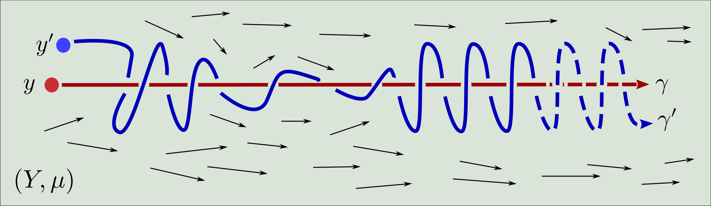
Figure 1. The function $\operatorname{ru}(\phi)$ at $y$ measures the time-averaged linking of the length $T$ trajectory $\gamma$ starting at $y$ and a nearby trajectory $\gamma^{\prime}$, as $T$ goes to $\infty$.

Since its introduction, the Ruelle invariant has appeared in low-dimensional dynamics (cf. Gambaudo-Ghys [11, 12, 13]), bifurcation theory (cf. Parlitz [26]) and Sturm-Liouville theory (cf. Schulz-Baldes [28, 29]). More recently, the Ruelle invariant has been applied very fruitfully to the study of 3-dimensional Reeb dynamics and 4-dimensional symplectic geometry [20, 5, 8].

In our previous work [5], we applied the Ruelle invariant to find the first examples of contact forms on the $3$-sphere that are dynamically convex in the sense of Hofer-Wysocki-Zehnder [19] but not symplectically convex (see Definition 1.10). This was a longstanding unsolved problem, and remains particularly impervious to more conventional modern methods in symplectic geometry such as Floer theory.

In this paper, we initiate the study of the Ruelle invariant in higher dimensional Reeb dynamics. Specifically, we construct a substantial generalization of the Ruelle invariant in [27] to symplectic cocycles of flows in any dimension. This generalization is related to previous ones such as the asymptotic Maslov index [7]. We then formulate and prove higher dimensional versions of results in [5], [20] and [8]. In particular, we show that dynamical convexity and symplectic convexity are inequivalent in all dimensions by constructing toric counter-examples, generalizing a construction of Dardennes-Gutt-Zhang [8] from dimension four.

1.1. Ruelle Invariant Of A Symplectic Cocycle

Let us begin by summarizing our construction of the Ruelle invariant and discussing its important formal properties.

Let $Y$ be a compact manifold equipped with an autonomous flow $\phi:\mathbb{R}\times Y\to Y$ and let $E\to Y$ be a symplectic vector bundle. Also let $\rho:\mathbb{R}\times Y\to Y$ denote the obvious projection.

Definition 1.1.

A symplectic cocycle $\Phi$ on $E$ for the flow $(Y,\phi)$ is a symplectic bundle map

(1.1) $$\Phi:\rho^{*}E\to\phi^{*}E\qquad\text{satisfying}\qquad\Phi(s+t,x)=\Phi(t,\phi(s,x))\Phi(s,x)$$

Fix a $\phi$-invariant Borel measure on $Y$, a symplectic cocycle $(E,\Phi)$ with vanishing first Chern class $c_{1}(E)$ and a homotopy class of trivialization $\tau:\Lambda E\simeq\mathbb{C}$ of the determinant line bundle $\Lambda E$. Here we consider the complex determinant line bundle with respect to an auxiliary choice of compatible complex structure on $E$ (see §3.1).

Theorem 1.2.

There is a well-defined Ruelle density and Ruelle invariant, denoted respectively by

$$\operatorname{ru}(\Phi,\tau)\in L^{1}(Y,\mu)\qquad\text{and}\qquad\operatorname{Ru}(\Phi,\tau,\mu):=\int_{Y}\operatorname{ru}(\Phi,\tau)\cdot\mu$$

Moreover, the Ruelle density and invariant satisfy the following properties.

• (Covariance) If $\Psi:(E,\Phi)\to(E^{\prime},\Phi^{\prime})$ is a symplectic cocycle isomorphism that maps $\tau$ to $\tau^{\prime}$, then

  $$\operatorname{ru}(\Phi,\tau)=\operatorname{ru}(\Phi^{\prime},\tau^{\prime})\qquad\qquad\operatorname{Ru}(\Phi,\tau,\mu)=\operatorname{Ru}(\Phi^{\prime},\tau^{\prime},\mu)$$

• (Direct Sum) If $\Phi=\Phi_{1}\oplus\Phi_{2}$ is a direct sum of symplectic cocycles and $\tau=\tau_{1}\otimes\tau_{2}$, then

  $$\operatorname{ru}(\Phi_{1}\oplus\Phi_{2},\tau_{1}\otimes\tau_{2})=\operatorname{ru}(\Phi_{1},\tau_{1})+\operatorname{ru}(\Phi_{2},\tau_{2})$$

• (Linearity) If $a\mu+b\nu$ is a positive combination of $\phi$-invariant Borel measures $\mu$ and $\nu$, then

  $$\operatorname{Ru}(\Phi,\tau,a\mu+b\nu)=a\operatorname{Ru}(\Phi,\tau,\mu)+b\operatorname{Ru}(\Phi,\tau,\nu)$$

• (Trivial Bundle) If $\Phi$ is a symplectic cocycle on $\mathbb{C}^{n}$ with the tautological trivialization $\tau_{\operatorname{std}}$, then

  $$\operatorname{ru}(\Phi,\tau_{\operatorname{std}})=\lim_{T\to\infty}\frac{q\circ\widetilde{\Phi}_{T}}{T}\qquad\qquad\operatorname{Ru}(\Phi,\tau_{\operatorname{std}})=\lim_{T\to\infty}\frac{1}{T}\int_{Y}q\circ\widetilde{\Phi}_{T}\cdot\mu$$

  Here $q$ is any rotation quasimorphism (see §2.2) and $\widetilde{\Phi}:\mathbb{R}\times Y\to\widetilde{\operatorname{Sp}}(2n)$ is the lift of $\Phi$ (regarded as a map $\mathbb{R}\times Y\to\operatorname{Sp}(2n)$) to the universal cover $\widetilde{\operatorname{Sp}}(2n)$.

The data needed to apply Theorem 1.2 arises in a fairly natural way for the dynamical systems that arise in symplectic geometry. Here are the main examples of interest.

Example 1.3 (Symplectic Flows).

Let $(X,\omega)$ be a symplectic manifold with a compact symplectic submanifold $\Sigma\subset X$ and let $V$ be a complete symplectic vector field tangent to $\Sigma$.

The differential of the symplectic flow $\Phi$ generated by $V$ induces a symplectic cocycle

$$T\Phi:\mathbb{R}\times TX\to\Phi^{*}TX$$

The flow $\Phi$ preserves $\Sigma$ since $V$ is tangent to $\Sigma$. Moreover, $\Sigma$ is equipped with the natural invariant measure $\omega^{m}|_{\Sigma}$ where $\operatorname{dim}(\Sigma)=2m$. Given a homotopy class of trivialization $\tau:\Lambda(TX)\simeq\mathbb{C}$ along $\Sigma$, we thus acquire a Ruelle density and invariant via Theorem 1.2.

$$\operatorname{ru}(T\Phi|_{\Sigma},\tau)\qquad\text{and}\qquad\operatorname{Ru}(T\Phi|_{\Sigma},\tau,\omega^{m}|_{\Sigma})$$

More generally, we only need to assume that the flow $\Phi$ is defined near $\Sigma$ and that $\Sigma$ is a (not necessarily symplectic) submanifold equipped with an invariant measure $\mu$. This special case is discussed in [7].

Example 1.4 (Hamiltonian Flows).

Let $X$ be a compact symplectic manifold with boundary and let $H:X\to\mathbb{R}$ be a Hamiltonian that is locally constant on $\partial X$. Assume that $c_{1}(X)=0$.

Then as a special case of Example 1.3, we get a Ruelle invariant associated to $X$, the flow $\Phi^{H}$ of $H$ and a chosen homotopy class of trivialization $\tau$. We denote this by

$$\operatorname{Ru}(X,H,\tau)\qquad\text{or simply }\quad\operatorname{Ru}(X,H)\quad\text{if}\quad H^{1}(X;\mathbb{Z})=0$$

Example 1.5 (Reeb Flows).

Recall that a contact $(2n-1)$-manifold $(Y,\xi)$ is a manifold equipped with a $(2n-2)$-plane field $\xi\subset TY$, called the contact structure, that is the kernel of a contact form $\alpha$. A contact form on $Y$ is a $1$-form that satisfies

$$\ker(d\alpha)\subset TY\text{ is rank 1}\qquad\text{and}\qquad\alpha|_{\ker(d\alpha)}>0$$

Every contact form comes equipped with a natural Reeb vector field $R$, defined by

$$\alpha(R)=1\qquad\iota_{R}d\alpha=0$$

The flow $\Phi:\mathbb{R}\times Y\to Y$ of the Reeb vector field is simply called the Reeb flow of $Y$. Note that $\Phi$ preserves $\alpha$ and the natural volume form $\alpha\wedge d\alpha^{n-1}$. The contact structure $\xi$ of $Y$ is a symplectic vector bundle with symplectic form $d\alpha|_{\xi}$. Thus

$$(\xi,T\Phi|_{\xi})$$

has the structure of a symplectic cocycle. If $\xi$ has vanishing first Chern class, we can choose a homotopy class of trivialization $\tau:\Lambda\xi\simeq\mathbb{C}$ to acquire a Ruelle invariant, denoted in this case by

$$\operatorname{Ru}(Y,\alpha,\tau)\qquad\text{or simply}\qquad\operatorname{Ru}(Y,\alpha)\quad\text{if}\quad H^{1}(Y;\mathbb{Z})=0$$

1.2. Ruelle Invariant Of Liouville Domains

In the case of Liouville domains, the Ruelle invariant yields a new symplectomorphism invariant (under some mild topological hypotheses).

Recall that a Liouville domain $(X,\lambda)$ is a compact symplectic manifold $(X,\omega)$ with a vector field $Z$ and a symplectically dual $1$-form $\lambda=\iota_{Z}\omega$ such that

$$\omega=d\lambda\qquad\text{and}\qquad Z\text{ points outward along }\partial X$$

The 1-form $\lambda$ and the vector field $Z$ are called the Liouville form and Liouville vector field of $X$. The skeleton $\operatorname{Skel}(X)$ of a Liouville domain $(X,\lambda)$ is the set given by

$$\operatorname{Skel}(X)=\bigcap_{t<0}\Phi^{Z}_{t}(X)\quad\text{where}\qquad\Phi^{Z}\text{ is the flow generated by }Z$$

The boundary $\partial X$ of a Liouville domain $X$ is a contact manifold with contact form $\lambda|_{\partial X}$. Moreover, $X$ admits a canonical Hamiltonian on the complement of the skeleton

$$H_{X}:X\setminus\operatorname{Skel}(X)\to(0,1]\qquad\text{characterized by}\qquad ZH_{X}=H_{X}\text{ and }H_{X}^{-1}(1)=\partial X$$

The level sets of $H_{X}$ are canonically contactomorphic to $\partial X$ and the Hamiltonian vector field of $H_{X}$ agrees with the Reeb vector field of $\lambda|_{\partial X}$ on each level. Note that $H_{X}$ extends continuously to the skeleton as $H_{X}|_{\operatorname{Skel}(X)}=0$, but in general this extension is not differentiable.

Figure 2. Some pictures of 2-dimensional Liouville domains. The skeleton is depicted in red and the Liouville vector field in blue.

Example 1.6 (Star-Shaped Domains).

A star-shaped domain $X\subset\mathbb{C}^{n}$ with smooth boundary $Y$ is a domain such that

$$0\in\operatorname{int}(X)\qquad\text{and}\qquad\text{the radial vector field }\partial_{r}\text{ is transverse to }Y$$

A star-shaped domain is naturally a Liouville domain, via restriction of the standard symplectic form and Liouville vector field on $\mathbb{C}^{n}$. In standard coordinates, these are given by

$$\omega=\sum_{j=1}^{n}dx_{j}\wedge dy_{j}\qquad\text{and}\qquad Z=\frac{1}{2}\sum_{j}x_{j}\partial_{x_{j}}+y_{j}\partial_{y_{j}}\qquad\text{where}\qquad z_{j}=x_{j}+i\cdot y_{j}$$

As with any Liouville domain, the restriction $\lambda|_{Y}$ of the Liouville form $\lambda=\iota_{Z}\omega$ is a contact form on the boundary $Y$. The Reeb vector field $R$ on $Y$ is given

$$R=\frac{J\nu}{\langle Z,\nu\rangle}\qquad\text{where }\nu\text{ is the normal vector field and }J\text{ is multiplication by }i$$

Strictly speaking, the Ruelle invariant of $H_{X}$ is not well-defined since $H_{X}$ is only defined away from $\operatorname{Skel}(X)$. However we can show that $\operatorname{ru}(X,H_{X})$ is invariant under $Z$. Thus we can take

$$\operatorname{Ru}(X,H_{X}):=\lim_{E\to 0}\;\operatorname{Ru}(X_{E},H_{X})\qquad\text{where}\qquad X_{E}=H_{X}^{-1}[E,1]$$

By applying a standard argument using Grey stability (cf. [5, Lemma 3.5] or [8, §3]) along with Stokes theorem, one may prove the following result.

Lemma 1.7.

Let $(X,\lambda)$ be a Liouville domain with $H^{1}(X;\mathbb{Z})=H^{2}(X;\mathbb{Z})=0$. Then

$$\operatorname{Ru}(X,H_{X})=\operatorname{Ru}(\partial X,\lambda|_{\partial X})$$

Furthermore, $\operatorname{Ru}(X,H_{X})=\operatorname{Ru}(W,H_{W})$ if $X$ and $W$ are symplectomorphic.

Thus the Ruelle invariant $\operatorname{Ru}(X)=\operatorname{Ru}(X,H_{X})$ is a symplectic invariant of Liouville domains.

Example 1.8 (Toric Domains).

In the case of a toric domain, we can prove an explicit formula for the Ruelle invariant that generalizes the formulas appearing in [20, 8].

Let $X_{\Omega}\subset\mathbb{C}^{n}$ be a smooth, star-shaped toric domain with moment region $\Omega\subset[0,\infty)^{n}$. Let $f_{\Omega}:[0,\infty)^{n}\to[0,\infty)$ be the unique smooth function such that

$$f^{-1}_{\Omega}[0,1]=\Omega\qquad\text{and}\qquad\sum_{i}x_{i}\cdot\partial_{i}f_{\Omega}=f_{\Omega}$$

Proposition 1.9.

(Proposition 5.6) The Ruelle invariant of $X_{\Omega}$ is given by the following formula.

$$\operatorname{Ru}(X_{\Omega})=\sum_{i}\int_{\Omega}\partial_{i}f_{\Omega}\cdot\operatorname{dvol}_{\mathbb{R}^{n}}$$

We will provide a review of toric domains and their Reeb dynamics in §5.

1.3. Symplectic Convexity

Our main application of the Ruelle invariant is to distinguish symplectically convex domains from dynamically convex domains. Let us recall the former concept.

Definition 1.10.

A star-shaped domain $X$ is symplectically convex if it is symplectomorphic to a convex star-shaped domain $X^{\prime}$.

Convex domains and their contact boundaries have many special properties that distinguish them from ordinary star-shaped domains and arbitrary contact forms on the sphere, particularly in dimension four (cf. [19, 31, 18]).

In [5], we demonstrated a new special property of the Ruelle invariant of convex star-shaped domains. To be precise, let $c(X)$ denote the period of the systole of $\partial X$, i.e.

(1.2) $$c(X):=\operatorname{min}\{T\;:\;T\text{ is the period of a closed Reeb orbit on }\partial X\}$$

Theorem 1.11.

[5] There are constants $C,c>0$ such that, for any convex star-shaped domain $X\subset\mathbb{C}^{2}$

$$c\cdot\operatorname{vol}(X)\leq\operatorname{Ru}(X)\cdot c(X)\leq C\cdot\operatorname{vol}(X)$$

Our second main result in this paper is the generalization of the upper bound in Theorem 1.11.

Theorem 1.12.

There is a constant $C(n)>0$ such that any convex star-shaped domain $X\subset\mathbb{C}^{n}$ satisfies

$$\operatorname{Ru}(X)\cdot c(X)\leq C(n)\cdot\operatorname{vol}(X)$$

Let us briefly sketch the proof, which is strategically similar to the proof of Theorem 1.11 in [5].

Proof Sketch. We start by observing that the tangent cocycle $T\Phi$ induced by the Hamiltonian flow $\Phi$ of $H_{X}$ is generated by the Hessian of $H_{X}$, in the sense that

$$\frac{d}{dt}(T\Phi)(t,x)=J\circ A(\Phi(t,x))\circ T\Phi(t,x)\qquad\text{where}\qquad A(x)=\nabla^{2}H_{X}(t,x)$$

General properties of the rotation quasimorphism (see §2.2) imply a trace estimate for the Ruelle invariant (see Proposition 3.13(e)) when the generator $A$ is positive semi-definite, which is the case if $X$ is convex. Thus we get

$$\operatorname{Ru}(X)\leq\frac{8n^{2}}{\pi}\cdot S(H_{X})\qquad\text{where}\qquad S(H_{X}):=\int_{X}\operatorname{tr}(A)\cdot\omega^{n}=\int_{X}\Delta H_{X}\cdot\omega^{n}$$

By analyzing the functional $S$, we prove (Proposition 4.10) that if $X$ and $W$ are sandwiched, in the sense that $W\subset X\subset c\cdot W$ for some constant $c\geq 1$, then

$$S(H_{X})\leq C(c,n)\cdot S(H_{W})\qquad\text{where $C(c,n)$ depends only on $n$ and $c$}$$

On the other hand, by the John ellipsoid theorem, we can find a standard symplectic ellipsoid $E$ such that $E\subset X\subset 2n\cdot E$ (after applying a symplectomorphism to $X$). For this ellipsoid, we have

$$c(X)\leq c(2n\cdot E)\qquad\operatorname{Ru}(X)\leq C^{\prime}(n)\cdot S(H_{2n\cdot E})\qquad\operatorname{vol}(2n\cdot E)\leq(2n)^{2n}\cdot\operatorname{vol}(X)$$

This reduces the proof to the statement that $S(H_{E})\cdot c(E)\leq C^{\prime\prime}(n)\cdot\operatorname{vol}(E)$ for any standard ellipsoid $E$ and a constant $C^{\prime\prime}(n)$ depending on $n$. This is a simple calculation (Lemma 4.14). ∎

We will carry our a detailed version of this proof (keeping track of constants) in §4.4.

Remark 1.13.

Our proofs of Theorem 1.12 above and Theorem 1.11 in [5] are very similar.

The key difference is our use of the Laplacian integral in place of the total mean curvature of the contact boundary, which plays an almost identical role in [5]. A higher dimensional bound by some extrinsic curvature integral (cf. [5, Lemma 3.11]) would, likely, further simplify and improve the proof of Theorem 1.12. At this time, we do not have a construction of the Ruelle invariant in higher dimensions that makes such a bound manifest.

Relatedly, the lower bound in Theorem 1.11 is likely true in higher dimensions. However, at this time, it is not clear how to adapt our methods to prove it. The proof in [5] relies on some delicate geometric reasoning specific to $\mathbb{C}^{2}$.

Remark 1.14.

The constant $C(n)$ in Theorem 1.12 can be given explicitly as

$$C(n):=2^{2n+5}\cdot n^{2n+3}\cdot\operatorname{exp}(8n^{4})$$

We believe that this constant is far from optimal. In fact, in dimension 4, it is an inferior constant to the one produced in the upper bound of Theorem 1.11 in [5].

1.4. Dynamical Convexity

Symplectic convexity is a mysterious and fundamentally extrisic condition that nonetheless plays a fundamental role in the symplectic geometry of star-shaped domains. One is thus drawn naturally to the following problem.

Problem 1.15.

Give a characterization of symplectic convexity in terms of symplectomorphism invariant properties, i.e. without referencing an embedding to $\mathbb{C}^{n}$.

A prominent candidate criterion to resolve Problem 1.15 was introduced by Hofer-Wysocki-Zehnder in their groundbreaking paper [19]. This characterization uses the lower-semicontinuous extension $\operatorname{LCZ}$ (see §2.3) of the Conley-Zehnder index $\operatorname{CZ}$, which can be viewed as a sort of Floer-theoretic Morse index of a closed Reeb orbit.

Definition 1.16.

A contact form on $\alpha$ on $S^{2n-1}$ is dynamically convex if

$$\operatorname{LCZ}(\gamma)\geq n+1\qquad\text{for every closed Reeb orbit }\gamma\text{ of }\alpha$$

Likewise, a star-shaped domain $(X,\lambda)$ is dynamically convex if $(\partial X,\lambda|_{\partial X})$ is.

Since [19], dynamical convexity has been used as a key hypothesis for many results in symplectic geometry (cf. [32, 33, 2, 3, 14, 10, 21]). It is simple to check that every strictly positively curved convex domain is dynamically convex, but the converse has been open for more than 20 years.

Question 1.17.

Is every dynamically convex contact form on $S^{2n-1}$ also convex?

In dimension four, we resolved this problem in [5] by constructing examples of dynamically convex contact manifolds violating both bounds in Theorem 1.11.

There was substantial evidence prior to [5] that the answer to Question 1.17 is no. For example, Abbondandolo-Bramham-Hryniewicz-Salomão proved in [1] that the weak Viterbo conjecture fails for dynamically convex domains. There is substantial evidence for the latter conjecture, especially in dimension four [6], so the contact forms in [1] are likely not convex.

In higher dimensions, Ginzburg-Macarini [15] constructed examples of dynamically convex contact forms admitting an action of a finite group $G$ that were not $G$-equivariantly isomorphic to a convex boundary with a similar $G$-action. However, their methods only apply when $G$ is non-trivial, and thus do not answer Question 1.17.

Theorem 1.12 can be used to resolve Question 1.17 in any dimension. In fact, using the results in [5], Dardennes-Gutt-Zhang [8] introduced an elegant toric construction of non-convex, dynamically convex domains in $\mathbb{C}^{2}$ that is much simpler than the open book construction in [5]. Using a straight forward adaptation of their operation, we prove the following result.

Proposition 1.18.

(Proposition 5.16) Let $X_{\Omega}$ be a star-shaped, concave toric domain. Then for any $C,\epsilon>0$, there is a smooth, star-shaped, concave moment region

$$\hat{\Omega}\supset\Omega$$

that satisfies the following properties

$$\operatorname{vol}(X_{\Omega})\leq\operatorname{vol}(X_{\hat{\Omega}})\leq\operatorname{vol}(X_{\Omega})+\epsilon\qquad\operatorname{Ru}(X_{\hat{\Omega}})\geq C\qquad c(X_{\Omega})\leq c(X_{\hat{\Omega}})$$

Smooth concave toric domains are examples of strictly monotone toric domains (see Definition 5.7), which are all dynamically convex (Proposition 5.8). Therefore, Proposition 5.16 resolves Question 1.17 as it implies the following corollary.

Corollary 1.19.

There are dynamically convex contact forms on $S^{2n-1}$ that are not symplectically convex.

Outline

This concludes the introduction §1. The rest of the paper is organized as follows.

In §2, we discuss preliminaries from symplectic linear algebra: the polar decomposition (§2.1), the rotation quasimorphism (§2.2) and Conley-Zehnder indices (§2.3-2.4).

In §3, we carry out the construction of the Ruelle invariant in detail. We start by discussing the construction of the rotation function via sub-additive ergodic theory (§3.1). Then we construct the Ruelle invariant and demonstrate its properties (§3.2).

In §4, we prove the main estimate on the Ruelle invariant. The begin with some preliminary estimates from Riemannian geometry (§4.1-4.2). We then review some properties of ellipsoids (§4.3) before proceeding to the main proof (§4.4).

In §5, we construct our toric counter-examples. First, we introduce toric domains and prove a Ruelle invariant formula (§5.1). We then discuss monotone (§5.2) and concave (§5.3) toric domains. Finally, we construct our counter-example in the last section of the paper (§5.4).

Acknowledgements

We would like to thank Lior Alon for helpful conversation. JC was supported by the National Science Foundation under Award No. 2103165.

2. Symplectic Linear Algebra

In this section, we review background topics from symplectic linear algebra that will be required later in the paper.

Specifically, we discuss polar decompositions and rotation quasimorphisms, which are key ingredients in our construction of the Ruelle invariant in §3. We also discuss variants and properties of the Conley-Zehnder index, which will be needed in §5.

2.1. Polar Decomposition

Recall that every matrix $A\in\operatorname{GL}(n,\mathbb{R})$ admits a unique polar decomposition into a product $A=UP$ where $U$ is orthogonal and $P$ is symmetric positive definite.

We can view the polar decomposition as pair of smooth maps between spaces of matrices.

(2.1) $$\Phi=(U,P):\operatorname{GL}(n)\to\operatorname{O}(n)\times\operatorname{P}(n)$$

Here $\operatorname{O}(n)$ and $\operatorname{P}(n)$ are, respectively, the spaces of orthogonal matrices and symmetric matrices.

$$\operatorname{O}(n)=\{A\in\operatorname{GL}(n)\;:\;AA^{T}=\operatorname{Id}\}\qquad\text{with Lie algebra}\qquad\mathfrak{o}(n)=\{A\in\mathfrak{gl}(2n)\;:\;A+A^{T}=0\}$$

$$\operatorname{P}(n):=\{A\in\operatorname{GL}(n)\;:\;A=A^{T}\}\qquad\text{with tangent space}\qquad\mathfrak{p}(n):=\{A\in\mathfrak{gl}(n)\;:\;A=A^{T}\}$$

We will need an explicit integral expression for the derivative of the polar decomposition.

Lemma 2.1.

The differential $TU:T\operatorname{GL}(n)\to T\operatorname{O}(n)$ of the map $U:\operatorname{GL}(n)\to\operatorname{O}(n)$ is given by

$$TU_{A}(UB)=U\cdot\int_{0}^{\infty}e^{-sP}(B-B^{T})e^{-sP}ds\quad\text{at}\quad A=UP$$

Proof.

Fix $A\in\operatorname{GL}(2n)$ and let $A=UP$ be the polar decomposition. Note that we can split the tangent space $T_{A}\operatorname{GL}(2n)$ into a direct sum

$$T_{A}\operatorname{GL}(2n)=\mathbb{R}^{n\times n}=U\cdot\mathfrak{o}(n)+U\cdot\mathfrak{p}(n)$$

That is, any matrix can be written as a sum $US+UT$ where $S$ is anti-symmetric and $T$ is symmetric. Clearly, if $T\in\mathfrak{p}(n)$ is a small symmetric matrix $T\in\mathfrak{p}(n)$, the unitary part of $U(P+T)$ is $U$. Thus, $U\cdot\mathfrak{p}(n)$ is the kernel of $TU_{A}$, and so

$$TU(UB)=TU_{A}(US)\qquad\text{where}\qquad S=\frac{1}{2}(B-B^{T})$$

Thus, we must compute $TU_{A}(US)$ where $S$ is the anti-symmetric part of $B$. Let

$$T\Phi_{A}(US)=(UM,N)\qquad\text{with}\qquad M\in\mathfrak{o}(n)\text{ and }N\in\mathfrak{p}(n)$$

denote the image of $US$ under $T\Phi_{A}$. Essentially by definition, $M$ and $N$ are the unique matrices that satisfy

$$US=T(\Phi^{-1})_{U,P}(UM,N)=\frac{d}{dt}(Ue^{Mt}P+U(P+tN))=UMP+UN$$

Multiplying this equation by $U^{-1}$ and taking the transpose, we acquire the two equations

$$S=MP+N\qquad\text{and}\qquad-S=-PM+N$$

The difference of these two equations is the well-known Lyupanov equation for $M$.

$$2S=\{M,P\}=MP+PM$$

This equation has an integral solution (cf. [24, Thm 12.3.3 and Thm 13.1.1]) given by

$$M=2\int_{0}^{\infty}e^{-Ps}Se^{-Ps}ds=\int_{0}^{\infty}e^{-Ps}(B-B^{T})e^{-Ps}ds$$

By construction of $M$, we have $TU_{A}(UB)=UM$, so this is the desired formula. ∎

We are, of course, mostly interested in the symplectic polar decomposition. Let $\Omega$ denote the standard linear symplectic structure on $\mathbb{C}^{n}\simeq\mathbb{R}^{2n}$, i.e.

$$\Omega=\left[\begin{array}[]{cc}0&-I_{n}\\ I_{n}&0\end{array}\right]$$

We abbreviate the group of linear symplectomorphisms on $(\mathbb{C}^{n},\Omega)$ and its Lie algebra in the usual way.

$$\operatorname{Sp}(2n)=\{A\in\operatorname{GL}(2n)\;:\;A\Omega A^{T}=\Omega\}\qquad\text{and}\qquad\mathfrak{sp}(2n)=\{A\in\mathfrak{gl}(2n)\;:\;A\Omega+\Omega A^{T}=0\}$$

Recall that $\mathfrak{sp}(2n)=\Omega\cdot\mathfrak{p}(2n)$ or, in other words, that $A$ is in the symplectic Lie algebra if and only if $\Omega A$ is symmetric. We let

$$\operatorname{U}(n)=\operatorname{O}(2n)\cap\operatorname{Sp}(2n)$$

denote the unitary group on $\mathbb{C}^{n}$. By standard linear algebra (cf. [25, Ch. 2]), the polar decomposition restricts to a map

$$(U,P):\operatorname{Sp}(2n)\to\operatorname{U}(n)\times(P(2n)\cap\operatorname{Sp}(2n))$$

The derivative formula in Lemma 2.1 implies an estimate for the trace of derivative of the polar decomposition. This will be a key ingredient for bounding the Ruelle invariant in §3.2.

Lemma 2.2 (Trace Estimate).

Let $A$ be a symplectic matrix and let $\Omega S$ be a symplectic Lie algebra element with $S$ positive semi-definite. Then

$$|\operatorname{tr}_{\mathbb{C}}(TU_{A}(\Omega SA)\cdot U^{-1})|\leq 16n^{2}\cdot\operatorname{tr}_{\mathbb{R}}(S)$$

Proof.

First, note that we can compute the complex trace as a real trace, as follows.

(2.2) $$\operatorname{tr}_{\mathbb{C}}(TU_{A}(\Omega SA)\cdot U^{-1})=2i\cdot\operatorname{tr}_{\mathbb{R}}(\Omega^{-1}\cdot TU_{A}(\Omega SA)\cdot U^{-1})$$

Thus it suffices to estimate the real trace of $\Omega^{-1}\cdot TU_{A}(\Omega SA)\cdot U^{-1}$. We may write $\Omega SA=UB$ where $B=U^{T}\Omega SUP$ and apply Lemma 2.1 to see that

$$TU_{A}(\Omega SA)=U\cdot\int_{0}^{\infty}e^{-sP}(U^{T}\Omega SUP+P^{T}U^{T}S\Omega U)e^{-sP}ds$$

We multiply on the left by $-\Omega$ and on the right by $U^{-1}=U^{T}$ to acquire the formula

(2.3) $$\Omega^{T}\cdot TU_{A}(\Omega SA)\cdot U^{T}=\int_{0}^{\infty}(\Omega^{T}Ue^{-sP}U^{T}\Omega)S(UPe^{-sP}U^{T})+(\Omega^{T}Ue^{-sP}PU^{T}\Omega)\Omega^{T}S\Omega(Ue^{-sP}U^{T})ds$$

The matrices $S,P$ and $e^{-sP}$ are all positive definite and $e^{-sP}$ has eigenvalues between $0$ and $1$. Thus, we may estimate the integrand on the righthand side as follows.

$$|\operatorname{tr}_{\mathbb{R}}((\Omega^{T}Ue^{-sP}U^{T}\Omega)S(UPe^{-sP}U^{T})+(\Omega^{T}Ue^{-sP}PU^{T}\Omega)\Omega^{T}S\Omega(Ue^{-sP}U^{T}))|$$

$$\leq|\operatorname{tr}_{\mathbb{R}}((\Omega^{T}Ue^{-sP}U^{T}\Omega)S(UPe^{-sP}U^{T}))|+|\operatorname{tr}_{\mathbb{R}}((\Omega^{T}Ue^{-sP}PU^{T}\Omega)\Omega^{T}S\Omega(Ue^{-sP}U^{T}))|$$

$$\leq 2\cdot\operatorname{tr}_{\mathbb{R}}(e^{-sP})\cdot\operatorname{tr}_{\mathbb{R}}(S)\cdot\operatorname{tr}(Pe^{-sP})\leq 4n\cdot\operatorname{tr}_{\mathbb{R}}(S)\cdot\operatorname{tr}(Pe^{-sP})$$

Therefore, we have

$$|\operatorname{tr}_{\mathbb{R}}(\Omega^{T}\cdot TU_{A}(\Omega SA)\cdot U^{T})\leq 4n\cdot\operatorname{tr}_{\mathbb{R}}(S)\cdot\big{(}\int_{0}^{\infty}Pe^{-sP}ds\big{)}=4n\cdot\operatorname{tr}_{\mathbb{R}}(S)\cdot\operatorname{tr}_{\mathbb{R}}(I_{2n})=8n^{2}\cdot\operatorname{tr}_{\mathbb{R}}(S)$$

We can plug this estimate into (2.2) to acquire the desired result. ∎

2.2. Rotation Quasimorphisms

The rotation quasimorphism is a certain (equivalence class of) quasimorphism on the universal cover $\widetilde{\operatorname{Sp}}(2n)$ of $\operatorname{Sp}(2n)$. Let us recall the relevant definitions.

Definition 2.3.

A quasimorphism $q:G\to\mathbb{R}$ from a group $G$ is a map that satisfies

(2.4) $$|q(gh)-q(g)-q(h)|<C\qquad\text{for all }g,h\in G\text{ and some }C>0\text{ independent of $g,h$}$$

Two quasimorphisms $q$ and $q^{\prime}$ are equivalent if $|q-q^{\prime}|$ is bounded, and $q$ is homogeneous if

$$q(g^{k})=k\cdot q(g)\qquad\text{for any}\qquad g\in G\qquad\text{and}\qquad k\in\mathbb{Z}$$

The universal cover of the symplectic group possesses a canonical homogeneous quasimorphism, due to the following result of Salamon-Ben Simon [30].

Theorem 2.4 ([30], Thm 1).

There exists a unique homogeneous quasimorphism

$$\rho:\widetilde{\operatorname{Sp}}(2n)\to\mathbb{R}$$

that restricts to the lift of the complex determinant $\operatorname{det}_{\mathbb{C}}$ on $\operatorname{U}(n)$. That is, the diagram

(2.5)       commutes.

Definition 2.5.

A rotation quasimorphism $q:\widetilde{\operatorname{Sp}}(2n)\to\mathbb{R}$ is a quasimorphism that is equivalent to the quasimorphism $\rho$ in Theorem 2.4.

We will use two representatives of this equivalence class of quasimorphisms. The first is defined using the complex determinant of the unitary part of the polar decomposition.

Example 2.6.

[4] The determinant quasimorphism $r:\widetilde{\operatorname{Sp}}(2n)\to\mathbb{R}$ is the lift of the composition

(2.6) $$\operatorname{Sp}(2n)\xrightarrow{U}\operatorname{U}(n)\xrightarrow{\text{det}_{\mathbb{C}}}\operatorname{U}(1)\simeq\mathbb{R}/\mathbb{Z}$$

Lemma 2.7.

[4, 9] There exists a constant $C>0$ such that

$$|r(\tilde{\Phi}\tilde{\Psi})-r(\tilde{\Phi})-r(\tilde{\Psi})|<C\qquad\text{for all}\qquad\tilde{\Phi},\tilde{\Psi}\in\widetilde{\operatorname{Sp}}(2n)$$

The second uses the eigenvalues of $A$, and appears in formulations of the Conley-Zehnder index.

Example 2.8.

[16] The eigenvalue quasimorphism $e:\widetilde{\operatorname{Sp}}(2n)\to\mathbb{R}$ is the lift of the map

$$\underline{e}:\operatorname{Sp}(2n)\to U(1)$$

defined as follows. Let $A$ be a symplectic matrix. For each eigenvalue $\lambda\in U(1)\setminus\{\pm 1\}$ with generalized complex eigenspace $V(\lambda)\subset\mathbb{C}^{2n}$, consider the real quadratic form

$$Q(A,\lambda):V(\lambda)\otimes V(\lambda)\to\mathbb{R}\qquad\text{given by}\qquad Q(A,\lambda)(v\otimes w)=\operatorname{Im}(\omega(v,\bar{w}))$$

Let $m(A,\lambda)$ be the maximal real dimension of a real subspace of $V(\lambda)$ on which $Q(A,\lambda)$ is positive definite. Finally, let $n(A)$ denote the sum of the complex dimensions of the generalized eigenspaces of $A$ with negative real eigenvalues. Then

(2.7) $$\underline{e}(A)=(-1)^{n(A)/2}\cdot\prod_{\lambda\in U(1)\setminus\{\pm 1\}}\lambda^{m(A,\lambda)/2}\in U(1)$$

Note that if $A$ has no eigenvalues in $(U(1)\cup(-\infty,0))\setminus\{1\}$, then $\underline{e}(A)$ is $1$ by convention.

Proposition 2.9 (Trace Estimate).

Let $A:[0,T]\to\operatorname{Sp}(2n)$ be a path of symplectic matrices with $A_{0}=\operatorname{Id}$ and let

$$S_{t}:=-\Omega\frac{dA}{dt}A_{t}^{-1}$$

Suppose that $S$ is positive semi-definite. Then the determinant quasimorphism $r$ (see Example 2.6) satisfies

$$r(A)\leq\frac{8n^{2}}{\pi}\int_{0}^{T}\operatorname{tr}(S_{t})dt$$

where we regard $A$ as an element of the universal cover $\widetilde{\operatorname{Sp}}(2n)$.

Proof.

Let $U$ be the unitary part of $A$. The rotation quasimorphism on $A$ is given by

$$r(A)=\frac{1}{2\pi i}\cdot\int_{0}^{T}\frac{\frac{d}{dt}(\text{det}_{\mathbb{C}}(U_{t}))}{\text{det}_{\mathbb{C}}(U_{t})}dt=\frac{1}{2\pi i}\cdot\int_{0}^{T}\text{tr}_{\mathbb{C}}(\frac{dU_{t}}{dt}U_{t}^{-1})dt$$

The trace estimate in Lemma 2.2 implies that the trace above can be estimated as

$$|\text{tr}_{\mathbb{C}}(\frac{dU_{t}}{dt}U_{t}^{-1})|\leq 16n^{2}\cdot\operatorname{tr}(S_{t})\qquad\text{and thus}\qquad|r(A)|\leq\frac{8n^{2}}{\pi}\cdot\int_{0}^{T}\operatorname{tr}(S_{t})ds\qed$$

2.3. Conley-Zehnder Index

The Conley-Zehnder index is an invariant of certain non-degenerate elements of the universal cover of the symplectic group.

Recall that a symplectic matrix $A\in\operatorname{Sp}(2n)$ is non-degenerate if none of its eigenvalues is equal to $1$. That is

$$\operatorname{det}(A-\operatorname{Id})\neq 0$$

We let $\operatorname{Sp}_{\star}(2n)\subset\operatorname{Sp}(2n)$ denote the open set of non-degenerate symplectic matrices and $\widetilde{\operatorname{Sp}}_{\star}(2n)$ denote its inverse image in the universal cover.

Theorem 2.10.

(cf. [16]) There is a unique continuous map, called the Conley-Zehnder index, of the form

$$\operatorname{CZ}:\widetilde{\operatorname{Sp}}_{\star}(2n)\to\mathbb{Z}\qquad\text{for each dimension $n$}$$

that satisfies the following list of axioms.

• (Naturality) $\operatorname{CZ}$ is invariant under conjugation.

  $$\operatorname{CZ}(\widetilde{\Psi}\widetilde{\Phi}\widetilde{\Psi}^{-1})=\operatorname{CZ}(\widetilde{\Phi})$$

• (Direct Sum) $\operatorname{CZ}$ is additive under direct sum.

  $$\operatorname{CZ}(\widetilde{\Phi}\oplus\widetilde{\Psi})=\operatorname{CZ}(\widetilde{\Psi})+\operatorname{CZ}(\widetilde{\Phi})$$

• (Maslov Index) If $\widetilde{\Psi}\in\pi_{1}(\operatorname{Sp}(2n))$ is an element of $\widetilde{\operatorname{Sp}}(2n)$ starting and ending on $\operatorname{Id}$, then

  $$\operatorname{CZ}(\widetilde{\Psi}\widetilde{\Phi})=2\mu(\widetilde{\Psi})+\operatorname{CZ}(\widetilde{\Phi})$$

  Here $\mu$ is the Maslov index of the loop (cf. [25]).

• (Signature) Let $\widetilde{\Psi}\in\widetilde{\operatorname{Sp}}_{\star}(2n)$ be the homotopy class of the path $t\mapsto\exp(2\pi\Omega At)$ for $t\in[0,1]$, where $A$ is a non-degenerate symmetric matrix with eigenvalues $\lambda$ of norm less than $1$. Then

  $$\operatorname{CZ}(\widetilde{\Psi})=\frac{1}{2}\cdot\operatorname{sign}(A)\qquad\text{where $\operatorname{sign}(\cdot)$ is the signature.}$$

There are a number of inequivalent ways to extend the Conley-Zehnder from $\widetilde{\operatorname{Sp}}_{\star}(2n)$ to $\widetilde{\operatorname{Sp}}(2n)$ [16, 14]. We are primarily interested in the following extension.

Definition 2.11.

The lower semi-continuous Conley-Zehnder index is the map

$$\operatorname{LCZ}:\widetilde{\operatorname{Sp}}(2n)\to\mathbb{Z}\qquad\text{with}\qquad\operatorname{LCZ}(\widetilde{\Phi})=\inf\big{\{}\liminf_{j\to\infty}\operatorname{CZ}(\widetilde{\Phi}_{j})\;:\;\widetilde{\Phi}_{j}\in\widetilde{\operatorname{Sp}}(2n)\text{ with }\widetilde{\Phi}_{j}\to\widetilde{\Phi}\big{\}}$$

Evidently, $\operatorname{CZ}$ extends $\operatorname{LCZ}$ in the sense that $\operatorname{CZ}=\operatorname{LCZ}$ on $\widetilde{\operatorname{Sp}}_{\star}(2n)$ and some axioms of $\operatorname{CZ}$ survive as properties of $\operatorname{LCZ}$. We record these properties, along with a key lower bound, below.

Lemma 2.12.

The lower semi-continuous Conley-Zehnder index $\operatorname{LCZ}$ has the following properties.

• (Naturality) $\operatorname{LCZ}$ is invariant under conjugation.

  $$\operatorname{LCZ}(\widetilde{\Psi}\widetilde{\Phi}\widetilde{\Psi}^{-1})=\operatorname{LCZ}(\widetilde{\Phi})$$

• (Direct Sum) $\operatorname{LCZ}$ is additive under direct sum.

  $$\operatorname{LCZ}(\widetilde{\Phi}\oplus\widetilde{\Psi})=\operatorname{LCZ}(\widetilde{\Psi})+\operatorname{CZ}(\widetilde{\Phi})$$

• (Maslov Index) If $\widetilde{\Psi}\in\pi_{1}(\operatorname{Sp}(2n))$ is an element of $\widetilde{\operatorname{Sp}}(2n)$ starting and ending on $\operatorname{Id}$, then

  $$\operatorname{LCZ}(\widetilde{\Psi}\widetilde{\Phi})=2\mu(\widetilde{\Psi})+\operatorname{LCZ}(\widetilde{\Phi})$$

• (Lower Bound) Let $\rho:\widetilde{\operatorname{Sp}}(2n)\to\mathbb{R}$ be the homogeneous rotation quasi-morphism. Then

  $$\operatorname{LCZ}(\widetilde{\Phi})\geq 2\cdot\rho(\widetilde{\Phi})-n$$

The naturality and Maslov index properties follow immediately from the same properties of $\operatorname{CZ}$. The direct sum property is [14, Lemma 4.3, p. 45] and the lower bound is given in [14, Eq. 4.6, p. 43]. Note that the lower bound in [14] is stated in terms of the mean index $\hat{\mu}$ (see [14, p. 41]).

As an example, we calculate $\operatorname{LCZ}$ in the case of paths in $U(1)$. We will use this calculation in §5.

Lemma 2.13.

Let $\widetilde{u}(\theta)\in\widetilde{\operatorname{Sp}}(2)$ for $\theta\in\mathbb{R}$ be the homotopy class of the path

$$[0,1]\to\operatorname{U}(1)\subset\operatorname{Sp}(2)\qquad\text{where}\qquad t\mapsto\operatorname{exp}(2\pi i\theta\cdot t)$$

Then $\operatorname{LCZ}(\widetilde{u}(\theta))$ is given by $2\lceil\theta\rceil-1$. As a special case, we have $\operatorname{LCZ}(\widetilde{\operatorname{Id}}_{2})=-1$.

Proof.

By the signature property in Theorem 2.10, we can directly compute that

$$\operatorname{CZ}(\widetilde{u}(\theta))=-1\text{ if }\theta\in(-1,0)\qquad\text{and}\qquad\operatorname{LCZ}(\widetilde{u}(\theta))=-1\text{ if }\theta=0$$

Since we can write $\theta=\lceil\theta\rceil+r$ for $r\in(-1,0]$, the Maslov index property then implies that

$$\operatorname{LCZ}(\widetilde{u}(\theta))=\operatorname{LCZ}(\widetilde{u}(\lceil\theta\rceil)\cdot\widetilde{u}(r))=2\mu(\widetilde{u}(\lceil\theta\rceil))+\operatorname{LCZ}(\widetilde{u}(r))=2\lceil\theta\rceil-1\qed$$

2.4. Indices Of Orbits

We conclude this section by discussing the Conley-Zehnder index of Hamiltonian and Reeb orbits.

Definition 2.14.

Let $X$ be a symplectic manifold with $c_{1}(TX)=0$ and let $H:X\to\mathbb{R}$ be a Hamiltonian. The (lower semi-continuous) Conley-Zehnder index

$$\operatorname{LCZ}(X,H;\gamma)\qquad\text{or simply}\qquad\operatorname{LCZ}(\gamma)$$

of a contractible periodic Hamiltonian orbit $\gamma:[0,T]\to X$ is defined as follows. Let $T\Phi$ be the differential of the Hamiltonian flow. Choose a disk $\Sigma\subset X$ bounded by $\gamma$ and a trivialization $\tau:TX|_{\Sigma}\simeq\mathbb{C}^{n}$. Let $\widetilde{\Psi}_{\tau}\in\widetilde{\operatorname{Sp}}(2n)$ be the homotopy class of the path

(2.8) $$\Psi_{\tau}:[0,T]\to\operatorname{Sp}(2n)\qquad\text{given by}\qquad\Phi_{\tau}(t)=\tau_{\gamma(t)}\circ T\Phi(t,z)\circ\tau_{\gamma(0)}^{-1}\in\operatorname{Sp}(2n)$$

We define $\operatorname{LCZ}(X,H;\gamma)$ to be $\operatorname{LCZ}(\widetilde{\Psi}_{\tau})$. Since $c_{1}(TX)=0$, this is independent of $\Sigma$.

Definition 2.15.

Let $(Y,\xi)$ be a closed contact manifold with $c_{1}(\xi)=0$ and let $\alpha$ be a contact form. The (lower semi-continuous) Conley-Zehnder index

$$\operatorname{LCZ}(Y,\alpha;\gamma)\qquad\text{or simply}\qquad\operatorname{LCZ}(\gamma)$$

of a contractible periodic Reeb orbit $\gamma:[0,T]\to Y$ is defined as follows. Let $T\Phi|_{\xi}$ be the differential of the Reeb flow restricted to $\xi$. Choose a disk $\Sigma$ bounded by $\gamma$ and a trivialization $\tau:\xi|_{\Sigma}\simeq\mathbb{C}^{n-1}$. Let $\widetilde{\Psi}_{\tau}\in\widetilde{\operatorname{Sp}}(2n-2)$ be the homotopy class of the path

(2.9) $$\Psi_{\tau}:[0,T]\to\operatorname{Sp}(2n)\qquad\text{given by}\qquad\Phi_{\tau}(t)=\tau_{\gamma(t)}\circ T\Phi|_{\xi}(t,y)\circ\tau_{\gamma(0)}^{-1}$$

We define $\operatorname{LCZ}(Y,\alpha;\gamma)$ to be $\operatorname{LCZ}(\widetilde{\Psi}_{\tau})$. Since $c_{1}(TX)=0$, this is independent of $\Sigma$.

In the case of a Liouville domain, these two versions of $\operatorname{LCZ}$ can be related.

Lemma 2.16.

Let $(X,\lambda)$ be a Liouville domain with boundary $(Y,\xi)$. Fix an contractible loop

$$\gamma:[0,T]\to Y=\partial X\qquad\text{with}\qquad\gamma(0)=\gamma(T)$$

that is an orbit of the canonical Hamiltonian $H_{X}$, or equivalently a Reeb orbit of $\lambda|_{Y}$. Then

$$\operatorname{LCZ}(X,H_{X};\gamma)=\operatorname{LCZ}(Y,\lambda|_{Y};\gamma)-1$$

Proof.

Let $Z$ and $R$ denote the Liouville and Hamiltonian vector field, respectively. Also, we adopt the shortened notation $H=H_{X}$. Note that we have a splitting

$$TX=\xi^{\omega}\oplus\xi=\operatorname{span}(Z,R)\oplus\xi\simeq\mathbb{C}\oplus\xi$$

Now choose a disk $\Sigma\subset Y$ bounded by $\gamma$ and let $\tau:\xi|_{\Sigma}\simeq\mathbb{C}^{n-1}$ be the unique isotopy class of trivialization of $\xi|_{\Sigma}$. Then we may form a trivialization $\sigma:TX|_{\Sigma}\simeq\mathbb{C}^{n}$ as the direct sum

$$\sigma=\tau_{\operatorname{std}}\oplus\tau:TX\simeq\mathbb{C}\oplus\xi\simeq\mathbb{C}^{n}\qquad\text{where}\qquad\tau_{\operatorname{std}}:\mathbb{C}\simeq\mathbb{C}\text{ is the tautological trivialization}$$

The flow $\Phi$ of $H$ preserves $Z$ and $R$. Indeed, $R$ generates $\Phi$, and since $ZH=H$ we have

$$dH=\mathcal{L}_{Z}(dH)=\mathcal{L}_{Z}(\iota_{R}\omega)=\iota_{[Z,R]}\omega+\iota_{R}\mathcal{L}_{Z}\omega=\iota_{[Z,R]}\omega+dH\qquad\text{and so}\qquad[R,Z]=0$$

Thus the paths $\Psi_{\sigma}:[0,T]\to\operatorname{Sp}(2n)$ in (2.8) and $\Psi_{\tau}:[0,T]\to\operatorname{Sp}(2n-2)$ in $(\ref{eqn:linearized_flow_Reeb})$ are related by

$$\Psi_{\sigma}=\operatorname{Id}_{2}\oplus\Psi_{\tau}\qquad\text{where}\qquad\operatorname{Id}_{2}:[0,T]\to\operatorname{Sp}(2)\text{ is the constant path}$$

By Lemma 2.13, we have $\operatorname{LCZ}(\widetilde{\operatorname{Id}}_{2})=-1$. Thus we have

$$\operatorname{LCZ}(X,H;\gamma)=\operatorname{LCZ}(\widetilde{\Psi}_{\sigma})=\operatorname{LCZ}(\widetilde{\operatorname{Id}}_{2})+\operatorname{LCZ}(\widetilde{\Psi}_{\tau})=-1+\operatorname{LCZ}(Y,\alpha;\gamma)\qed$$

As a corollary, we have a different characterization of dynamical convexity in terms of the Hamiltonian flow of the canonical Hamiltonian.

Corollary 2.17.

A star-shaped domain $X\subset\mathbb{C}^{n}$ is dynamically convex if and only if the closed orbits $\gamma$ of the canonical Hamiltonian $H_{X}$ satisfy

$$\operatorname{LCZ}(X,H_{X};\gamma)\geq n$$

3. Ruelle Density And Invariant

In this section, we construct the Ruelle invariant of a symplectic cocycle of a flow on a compact manifold, and demonstrate its basic properties.

3.1. Rotation Function

For the rest of the section, we fix a flow and a symplectic cocycle.

$$\phi:\mathbb{R}\times Y\to Y\qquad\Phi:\rho^{*}E\to\phi^{*}E$$

We also fix a $\phi$-invariant Borel measure $\mu$. Our construction of the Ruelle invariant requires an auxilliary family of maps

$$\tilde{u}_{T}:Y\to\mathbb{R}\qquad\text{also denoted by}\qquad\tilde{u}_{T}(\Phi;J,\tau):Y\to\mathbb{R}\qquad\text{for }T\in[0,\infty)$$

depending on a choice of complex structure $J$ and trivialization $\tau$. We refer to $\tilde{u}_{T}$ as the rotation function at time $T$. The goal of this subsection is to define the rotation function and prove some basic properties.

Let us, first, recall the definitions of the various auxilliary data required to build $\tilde{u}_{T}$.

Definition 3.1.

A (compatible) complex structure $J$ on $E$ is an bundle map $J:E\to E$ such that

$$J^{2}=-\operatorname{Id}\qquad\text{and}\qquad\omega(J-,-)\text{ is a fiberwise inner product}$$

A choice of compatible complex structure $J$ gives $E$ the structure of a Hermitian vector bundle. Standard results in algebraic topology (cf. [25]) state that the space $\mathcal{J}(E,\omega)$ of compatible complex structures on $E$ is contractible. Moreover, any two choices $J,J^{\prime}$ of such complex structures yield isomorphic Hermitian vector bundles $(E,\omega,J)\simeq(E,\omega,J^{\prime})$.

Definition 3.2.

The determinant bundle $\Lambda E$ of $(E,J)$ is the maximal wedge power of $E$ as a complex vector bundle. That is

$$\Lambda E:=\wedge^{k}\big{(}E\big{)}\qquad\text{where}\qquad k=\operatorname{rank}_{\mathbb{C}}(E)$$

A trivialization $\tau:\Lambda E\simeq\mathbb{C}$ is a unitary bundle map to the trivial bundle.

The determinant bundle of $E$ is independent of $J$ up to (homotopically unique) isomorphism. In particular, the set of homotopy classes of trivialization

$$\mathcal{T}(\Lambda E):=\{\text{trivializations }\tau:\Lambda E\simeq\mathbb{C}\}\;\big{/}\text{ homotopy }$$

is well-defined, without reference to a specific choice of $J$. The determinant bundle admits a trivialization if and only if $c_{1}(E)=c_{1}(\Lambda E)=0$. Furthermore, the space of trivializations is naturally a torsor over $[Y,S^{1}]\simeq H^{1}(Y;\mathbb{Z})$.

We are now ready to proceed with the construction of the rotation function.

Construction 3.3.

Choose a compatible complex structure $J$ on $E$ and an explicit unitary trivialization $\tau:\Lambda E\simeq\mathbb{C}$ in the chosen class. Start by taking the polar decomposition of $\Phi$

$$\Phi:\rho^{*}E\xrightarrow{P}\rho^{*}E\xrightarrow{U}\phi^{*}E$$

Here $P$ is self-adjoint and $U$ is unitary with respect to $\omega$ and $J$. The determinant $\Lambda U$ of $U$ and the trivialization $\tau$ determine a unitary bundle map

$$u:\mathbb{C}\xrightarrow{\tau^{-1}}\rho^{*}\Lambda E\xrightarrow{\Lambda U}\phi^{*}\Lambda E\xrightarrow{\tau}\mathbb{C}\quad\text{or equivalently a map}\quad u:\mathbb{R}\times Y\to U(1)$$

The map $u$ sends $0\times Y$ to $1\in U(1)$, and is therefore null-homotopic. Thus there is a unique lift

$$\tilde{u}:\mathbb{R}\times Y\to\mathbb{R}\qquad\text{such that}\qquad\exp(2\pi i\cdot\tilde{u})=u\quad\text{and}\quad\tilde{u}|_{0\times Y}=0$$

The rotation function $\tilde{u}_{T}$ is simply this lift at time $T$, i.e. $\tilde{u}(T,-)$.

We may view these maps as a version of the rotation quasimorphism applied pointwise in $Y$ to $\Phi$. To make this precise, it will be helpful to fix some notation.

Notation 3.4.

Given a trajectory $\gamma:[0,T]\to Y$ of $\phi$ and a trivialization $\Xi:E|_{\gamma}\simeq\mathbb{C}^{n}$, we let

$$\Phi_{\Xi}:[0,T]\to\operatorname{Sp}(2n)\qquad\text{denote the map}\qquad\Phi_{\Xi}(t):=\Xi(t)\circ\Phi(t,x)\circ\Xi(0)^{-1}$$

Furthermore, we let $\tilde{\Phi}_{\Xi}$ denote the unique lift of $\Phi_{\Xi}$ to the universal cover satisfying $\tilde{\Phi}_{\Xi}(0)=\tilde{\operatorname{Id}}$.

Lemma 3.5 (Quasimorphism).

Let $\gamma:[0,T]\to Y$ be a trajectory of $\phi$ with $\gamma(0)=X$ and let $\Xi:E|_{\gamma}\simeq\mathbb{C}^{n}$ be a unitary trivialization of $E$ over $\gamma$ such that the map $\Lambda\Xi:\Lambda E|_{\gamma}\simeq\mathbb{C}$ is $\tau|_{\gamma}$. Then

$$\tilde{u}_{T}(x)=r(\widetilde{\Phi}_{\Xi})$$

Proof.

Since $\Xi$ is unitary, the unitary parts $U_{\Xi}$ of $\Phi_{\Xi}$ and $U$ of $\Phi$ are related by

$$U_{\Xi}(t):=\Xi(t)\circ U(t,x)\circ\Xi(0)^{-1}\in\operatorname{Sp}(2n)$$

The map on the determinant bundle $\Lambda\mathbb{C}^{n}=\mathbb{C}$ induced by $U_{\Xi}$ is simply the determinant over $\mathbb{C}$. In particular, we have

$$\operatorname{det}_{\mathbb{C}}(U_{\Xi}(t))=\Lambda\Xi(t)\circ\Lambda U(t,x)\circ\Lambda\Xi(0)^{-1}=\tau(\phi(t,x))\circ\Lambda U(t,x)\circ\tau^{-1}(x)=u(t,x)$$

In particular, the maps $r\circ\widetilde{\Phi}_{\Xi}:[0,T]\to\mathbb{R}$ and $\tilde{u}(x):[0,T]\to\mathbb{R}$ are both lifts of the same map $[0,T]\to U(1)$ that are $0$ at $t=0$. This implies that they agree, proving the result. ∎

The rotation functions at time $T$ essentially define a sub-additive process in the sense of Kingman [23]. We use the following definition, which specializes the one in [23] to our setting.

Definition 3.6.

A sub-additive process $f_{T}:Y\to\mathbb{R}$ for $T\in[0,\infty)$ for the dynamical system $(Y,\phi)$ with invariant measure $\mu$ is a family of $\mu$-integrable functions that, for some $C>0$, satisfy

$$f_{S+T}\leq f_{S}+\phi^{*}_{S}f_{T}+C\qquad\qquad\int_{Y}f_{T}\cdot\mu\geq-C\cdot T\qquad\qquad\int_{Y}\big{(}\sup_{0\leq S\leq 1}|f_{S}|\big{)}\cdot\mu<\infty$$

Lemma 3.7.

The family of maps $\tilde{u}_{T}$ are a sub-additive process for $(Y,\phi)$ and $\mu$.

Proof.

We verify the properties in Definition 3.6. For the first property, fix a trajectory $\gamma:[0,S+T]\to Y$ of $\phi$ with $\gamma(0)=x$, and choose a unitary trivialization $\Xi:E|_{\gamma}\simeq\mathbb{C}^{n}$ inducing the trivialization $\tau:\Lambda E\simeq\mathbb{C}$. Define

(3.1) $$\Phi_{\Xi}:[0,S+T]\to\operatorname{Sp}(2n)\qquad\Phi_{\Xi}(t):=\Xi(t)\circ\Phi(t,x)\circ\Xi(0)^{-1}$$

Let $\tilde{\Phi}_{\Xi}:[0,S+T]\to\widetilde{\operatorname{Sp}}(2n)$ denote the lift to the universal cover. Then by Lemma 3.5 and the quasimorphism property of $r$, there is a constant $c>0$ such that

(3.2) $$\tilde{u}_{S+T}(x)=r(\tilde{\Phi}_{\Xi}(S+T))\leq r(\tilde{\Phi}_{\Xi}(S))+r(\tilde{\Phi}_{\Xi}(S+T)\tilde{\Phi}_{\Xi}(S)^{-1})+C$$

Clearly $\tilde{u}_{S}(x)=r(\tilde{\Phi}_{\Xi}(S))$ by Lemma 3.5. Moreover, the cocycle property of $\Phi$ implies that

$$\Phi_{\Xi}(S+t)\Phi_{\Xi}(S)^{-1}=\Xi(t)\circ\Phi(S+t,x)\circ\Phi(S,x)\circ\Xi(s)=\Xi(S+t)\circ\Phi(t,\phi_{S}(t))\circ\Xi(S)^{-1}$$

Thus Lemma 3.5 also implies that $\phi^{*}_{S}\tilde{u}_{T}(x)=r(\tilde{\Phi}_{\Xi}(S+T)\tilde{\Phi}_{\Xi}(S)^{-1})$. The first property in Definition 3.6 then follows from (3.2). To see the second property, note that if $T=m+S$ for $S\in[0,1]$, we have

$$\int_{Y}\tilde{u}_{T}\cdot\mu\geq\sum_{k=0}^{m-1}\int_{Y}\phi^{*}_{k}\tilde{u}_{1}\cdot\mu+\int_{Y}\phi^{*}_{m}\tilde{u}_{S}\cdot\mu-cm\geq(-c+M\cdot\mu(Y))\cdot T$$

Here $M$ is the minimum of $\tilde{u}_{T}$ for $T\in[0,1]$ and $0$. We can thus take the constant in the lemma to be $c-M\cdot\mu(Y)$. Finally, the third property follows immediately from the fact that $\tilde{u}:[0,1]\times Y\to\mathbb{R}$ is continuous and $Y$ is compact. ∎

In [23], Kingman proves several ergodic theorems, one of which can be stated as follows.

Theorem 3.8 ([23], Thm 4).

Let $f_{T}$ be a sub-additive process in the sense of Definition 3.6. Then $\frac{f_{T}}{T}$ converges in $L^{1}(Y,\mu)$ and pointwise almost everywhere as $T\to\infty$.

Applying Theorem 3.8 to $\tilde{u}$ via Lemma 3.7, we immediately acquire the following result.

Corollary 3.9.

The family of maps $\frac{\tilde{u_{T}}}{T}$ converges in $L^{1}(Y,\mu)$ and pointwise almost everywhere as $T\to\infty$.

Critically, the limit of $\frac{\tilde{u}_{T}}{T}$ is independent of the auxilliary choices made. To demonstrate this, we need the following lemma.

Lemma 3.10 (Automorphism).

There is a constant $C>0$ with the property that, if $\Psi:Y\to\operatorname{Aut}(E)$ is a symplectic bundle map homotopic to $\operatorname{Id}$, then

$$|\tilde{u}_{T}(\Psi^{*}\Phi;J,\tau)-\tilde{u}_{T}(\Phi;J,\tau)|\leq C$$

Proof.

Let $\tilde{\Psi}:Y\to\widetilde{\operatorname{Aut}}(E)$ denote any lift of $\Psi$ to the (fiberwise) universal cover bundle $\widetilde{\operatorname{Aut}}(E)$ of $\operatorname{Aut}(E)$. Fix a trajectory $\gamma:[0,T]\to Y$ of $\phi$ with $\gamma(0)=x$, and choose a unitary trivialization $\Xi:E|_{\gamma}\simeq\mathbb{C}^{n}$ with $\Lambda\Xi=\tau$. Let $\Phi_{\Xi}$ and $\Psi^{*}\Phi_{\Xi}$ be defined as in Notation 3.4, and let

$$\Psi_{\Xi}:[0,T]\to\operatorname{Sp}(2n)\quad\text{denote}\quad\Psi_{\Xi}(t):=\Xi(t)\circ\Psi(\gamma(t))\circ\Xi(t)^{-1}$$

Note that $\Phi_{\Xi}$, $\Psi^{*}\Phi_{\Xi}$ and $\Psi_{\Xi}$ are all related by the following identity.

(3.3) $$\Psi^{*}\Phi_{\Xi}(t)=\Psi_{\Xi}(t)\Phi_{\Xi}(t)\Psi_{\Xi}(t)^{-1}$$

The trivialization induces a bundle isomorphism $\gamma^{*}\widetilde{\operatorname{Aut}}(E)\simeq\widetilde{\operatorname{Sp}}(2n)$, and thus the lift $\tilde{\Psi}$ of $\Psi$ induces a unique lift $\tilde{\Psi}_{\Xi}$ of $\Psi_{\Xi}$. The identity (3.3) lifts to

(3.4) $$\widetilde{\Psi^{*}\Phi}_{\Xi}(t)=\tilde{\Psi}_{\Xi}(t)\tilde{\Phi}_{\Xi}(t)\tilde{\Psi}_{\Xi}(t)^{-1}$$

Indeed, it suffices to check (3.4) at $t=0$, where both sides are $\tilde{\operatorname{Id}}\in\widetilde{\operatorname{Sp}}(2n)$.

To acquire the desired conclusion from (3.4), we note that by Lemma 3.5, we have

(3.5) $$\tilde{u}_{T}(\Psi^{*}\Phi;J,\tau)=r\circ\widetilde{\Psi^{*}\Phi}_{\Xi}(T)\qquad\text{and}\qquad\tilde{u}_{T}(\Phi;J,\tau)=r\circ\widetilde{\Phi}_{\Xi}(T)$$

On the other hand, let $c>0$ be constant in Lemma 2.7. Then

$$|r\circ\tilde{\Psi}_{\Xi}+r\circ\tilde{\Psi}^{-1}_{\Xi}|\leq|r(\tilde{\operatorname{Id}})|+c=c$$

Therefore, at time $T$ we have the following inequality.

$$|r(\widetilde{\Psi^{*}\Phi}_{\Xi}(T))-r(\tilde{\Phi}_{\Xi}(T))|\leq|r(\widetilde{\Phi}_{\Xi}(T))+r(\tilde{\Psi}_{\Xi})+r(\tilde{\Psi}^{-1}_{\Xi})-r(\tilde{\Phi}_{\Xi}(T))|+2c\leq 3c$$

The result now follows from (3.5) by taking $C=3c$. ∎

Proposition 3.11.

The limit of $\frac{\tilde{u}_{T}}{T}$ as $T\to\infty$ is independent of $J$ and the choice of representative of $\tau$.

Proof.

For convenience, we fix the following notation for this proof.

$$g(\Phi,J,\tau):=\lim_{T\to\infty}\frac{\tilde{u}_{T}(\Phi,J,\tau)}{T}\in L^{1}(Y,\mu;\mathbb{R})$$

To show that the limit depends only on the isotopy class of $\tau$, let $\sigma:\Lambda E\simeq\mathbb{C}$ and $\tau:\Lambda E\simeq\mathbb{C}$ be isotopic unitary trivializations. Then we have

$$\sigma=f\tau\qquad\text{where}\qquad f:X\to U(1)\qquad\text{satisfies}\qquad[f]=0\in[Y,U(1)]$$

Since $f$ is null-homotopic, $f$ admits a lift $\tilde{f}:Y\to\mathbb{R}$ via the covering map $\exp(2\pi i\cdot):\mathbb{R}\to U(1)$. We can then relate $u_{T}(\Phi,J,\tau)$ and its lift to $u_{T}(\Phi,J,\sigma)$ by the following formulas.

(3.6) $$u_{T}(\Phi,J,\sigma)=(f\circ\phi)u_{T}(\Phi,J,\tau)f^{-1}\qquad\text{and}\qquad\tilde{u}_{T}(\Phi,J,\sigma)=\tilde{f}\circ\phi+\tilde{u}_{T}(\Phi,J,\tau)-\tilde{f}$$

The first formula in (3.6) follows directly from the definition, while the second follows from the uniqueness of the lift that is $0$ along $0\times Y$. We then see that

$$\|g(\Phi,J,\tau)-g(\Phi,J,\sigma)\|_{L^{1}}=\lim_{T\to\infty}\frac{1}{T}\|\tilde{u}_{T}(\Phi,J,\sigma)-\tilde{u}_{T}(\Phi,J,\tau)\|_{L^{1}}$$

$$=\lim_{T\to\infty}\frac{1}{T}\|\tilde{f}\circ\phi_{t}-\tilde{f}\|_{L^{1}}\leq\lim_{T\to\infty}\frac{2\|\tilde{f}\|_{L^{1}}}{T}=0$$

Thus $g(\Phi,J,\tau)=g(\Phi,J,\sigma)$ in $L^{1}(Y,\mu;\mathbb{R})$ and the limit depends only the class of $\tau$.

To prove independence of $J$, let $I$ and $J$ be two choices of compatible complex structure on $E$. There is a unitary bundle isomorphism

$$\Psi:Y\to\operatorname{Aut}(E)\qquad\text{such that}\qquad\Psi^{*}\omega=\omega\qquad\Psi^{*}J=I\quad\text{and}\quad\Psi\sim\operatorname{Id}_{E}$$

Here $\Psi$ is homotopic to the identity through symplectic bundle automorphisms. In particular, $\Psi^{*}\tau=\tau$ for any trivialization class $\tau$. Since the limit depends only on the trivialization homotopy class, we thus have

$$g(\Phi,J,\tau)=g(\Psi^{*}\Phi,\Psi^{*}J,\Psi^{*}\tau)=g(\Psi^{*}\Phi,I,\tau)$$

Using this identity and Lemma 3.10, we compute

$$\|g(\Phi,J,\tau)-g(\Phi,I,\tau)\|_{L^{1}}\leq\lim_{T\to\infty}\frac{1}{T}\|\tilde{u}_{T}(\Psi^{*}\Phi,I,\tau)-\tilde{u}_{T}(\Phi,I,\tau)\|_{L^{1}}\leq\lim_{T\to\infty}\frac{C\cdot\mu(Y)}{T}=0$$

This proves that the limit is independent of $J$ and concludes the proof.∎

3.2. Construction Of Invariant

We are now ready to give a precise definition of the Ruelle density and invariant. Choose a complex structure $J$ and trivialization in class $\tau$, as in §3.1.

Definition 3.12.

The Ruelle density $\operatorname{ru}(\Phi,\tau)$ and the Ruelle invariant $\operatorname{Ru}(\Phi,\tau)$ are defined by

$$\operatorname{ru}(\Phi,\tau):=\lim_{T\to\infty}\frac{\tilde{u}_{T}}{T}\qquad\text{and}\qquad\operatorname{Ru}(\Phi,\tau):=\int_{Y}\operatorname{ru}(\Phi,\tau)\cdot\mu$$

Proposition 3.13.

The Ruelle density and the Ruelle invariant satisfy the following formal properties.

• (Covariance) If $\Psi:(E,\Phi)\to(E^{\prime},\Phi^{\prime})$ is a symplectic cocycle isomorphism that maps $\tau$ to $\tau^{\prime}$, then

  $$\operatorname{ru}(\Phi,\tau)=\operatorname{ru}(\Phi^{\prime},\tau^{\prime})\qquad\qquad\operatorname{Ru}(\Phi,\tau,\mu)=\operatorname{Ru}(\Phi^{\prime},\tau^{\prime},\mu)$$

• (Direct Sum) If $\Phi=\Phi_{1}\oplus\Phi_{2}$ is a direct sum of symplectic cocycles and $\tau=\tau_{1}\otimes\tau_{2}$, then

  $$\operatorname{ru}(\Phi_{1}\oplus\Phi_{2},\tau_{1}\otimes\tau_{2})=\operatorname{ru}(\Phi_{1},\tau_{1})+\operatorname{ru}(\Phi_{2},\tau_{2})$$

• (Linearity) If $a\mu+b\nu$ is a positive combination of $\phi$-invariant Borel measures $\mu$ and $\nu$, then

  $$\operatorname{Ru}(\Phi,\tau,a\mu+b\nu)=a\operatorname{Ru}(\Phi,\tau,\mu)+b\operatorname{Ru}(\Phi,\tau,\nu)$$

• (Trivial Bundle) If $\Phi$ is a symplectic cocycle on $\mathbb{C}^{n}$ with the tautological trivialization $\tau_{\operatorname{std}}$, then

  $$\operatorname{ru}(\Phi,\tau_{\operatorname{std}})=\lim_{T\to\infty}\frac{q\circ\widetilde{\Phi}_{T}}{T}\qquad\qquad\operatorname{Ru}(\Phi,\tau_{\operatorname{std}})=\lim_{T\to\infty}\frac{1}{T}\int_{Y}q\circ\widetilde{\Phi}_{T}\cdot\mu$$

  Here $q$ is any rotation quasimorphism (see §2.2) and $\widetilde{\Phi}:\mathbb{R}\times Y\to\widetilde{\operatorname{Sp}}(2n)$ is the lift of $\Phi$ (regarded as a map $\mathbb{R}\times Y\to\operatorname{Sp}(2n)$) to the universal cover $\widetilde{\operatorname{Sp}}(2n)$.

Proof.

These properties are more or less immediate from the properties of $\tilde{u}_{T}$. We discuss each proof separately below.

Covariance. This is immediate since we can assume (by choice of $J^{\prime}$ and $\tau^{\prime}$) that $\Psi$ is unitary.

Direct Sum. Choose explicit complex structures $J_{i}$ and unitary trivializations $\tau_{i}:\Lambda E_{i}\simeq\mathbb{C}$. We adopt the notatation

$$E=E_{1}\oplus E_{2}\qquad\Phi=\Phi_{1}\oplus\Phi_{2}\qquad J=J_{1}\oplus J_{2}\qquad\tau=\tau_{1}\otimes\tau_{2}$$

The unitary part $U$ of the cocycle $\Phi$ with respect to $J$ and the determinant $\Lambda U$ can be written in terms of the unitary parts $U_{i}$ of $\Phi_{i}$ as

$$U=U_{1}\oplus U_{2}\qquad\Lambda U=\Lambda U_{1}\otimes\Lambda U_{2}$$

Therefore, the induced maps $Y\to U(1)$ satisfy the following identities.

$$u(\Phi,J,\tau)=u(\Phi_{1},J_{1},\tau_{1})u(\Phi_{2},J_{2},\tau_{2})\qquad\text{and}\qquad\tilde{u}(\Phi,J,\tau)=\tilde{u}(\Phi_{1},J_{1},\tau_{1})+\tilde{u}(\Phi_{2},J_{2},\tau_{2})$$

The additivity of the Ruelle density and invariant now follows directly from the definition.

Linearity. This follows from the fact that $\operatorname{ru}(\Phi,\tau)\in L^{1}(Y,\mu)\cap L^{1}(Y,\nu)$ and the linearity of integration against measures.

Trivial Bundle. Clearly, it suffices to prove the result for the rotation quasimorphism $r$. Let $\tilde{\Phi}:\mathbb{R}\times Y\to\widetilde{\operatorname{Sp}}(2n))$ denote the lift of $\Phi:\mathbb{R}\times Y\to\operatorname{Sp}(2n)$ to the universal cover. Let $\Xi:\mathbb{C}^{n}\to\mathbb{C}^{n}$ be the identity trivialization on $\mathbb{C}^{n}$, so that

$$\Phi_{\Xi}=\Phi\qquad\text{and}\qquad\Lambda\Xi=\tau_{\operatorname{std}}$$

Then by Lemma 3.5, we have

$$\tilde{u}_{T}(x)=r\circ\tilde{\Phi}(T,x)$$

The result now follows immediately from the definition of $\operatorname{ru}$ and $\operatorname{Ru}$. ∎

As an easy consequence of Proposition 3.13(d) and Proposotion 2.9, we acquire a key trace bound on the Ruelle invariant.

Lemma 3.14 (Trace Bound).

Let $\Phi$ be a symplectic cocycle on $\mathbb{C}^{n}$ generated by a map $A:Y\to\mathfrak{sp}(2n)$. That is

$$\frac{d}{dt}\big{(}\Phi(t,x)\big{)}=A(\phi(t,x))\circ\Phi(t,x)$$

Assume that $-\Omega A$ is positive semi-definite, where $\Omega$ is the matrix representing the standard symplectic form. Then

$$\operatorname{Ru}(\Phi,\tau_{\operatorname{std}})\leq\frac{8n^{2}}{\pi}\cdot\int_{Y}\operatorname{tr}(-\Omega A)\cdot\mu$$

Proof.

By Proposition 3.13(d) and Proposition 2.9, we know that

(3.7) $$\operatorname{Ru}(\Phi,\tau,\mu)=\lim_{T\to\infty}\frac{1}{T}\int_{Y}r\circ\widetilde{\Phi}_{T}\cdot\mu\leq\frac{8n^{2}}{\pi}\lim_{T\to\infty}\frac{1}{T}\int_{Y}\Big{(}\int_{0}^{T}\operatorname{tr}(-\Omega A(\phi(t,x)))\cdot dt\Big{)}\mu$$

Rearranging the order of integration and using the fact that $\phi$ is measure preserving, we see that

$$\int_{Y}\Big{(}\int_{0}^{T}\operatorname{tr}(-\Omega A(\phi(t,x)))\cdot dt\Big{)}\mu=\int_{0}^{T}\Big{(}\int_{Y}\phi^{*}_{t}\operatorname{tr}(-\Omega A)\cdot\mu\Big{)}dt=\int_{0}^{T}\Big{(}\int_{Y}\operatorname{tr}(-\Omega A)\cdot\mu\big{)}\cdot dt$$

Therefore, the right hand side of (3.7) simplifies to

$$\frac{8n^{2}}{\pi}\lim_{T\to\infty}\frac{1}{T}\int_{Y}\Big{(}\int_{0}^{T}\operatorname{tr}(-\Omega A(\phi(t,x)))\cdot dt\Big{)}\mu=\frac{8n^{2}}{\pi}\lim_{T\to\infty}\frac{1}{T}\int_{0}^{T}\Big{(}\int_{Y}\operatorname{tr}(-\Omega A)\cdot\mu\big{)}\cdot dt=\frac{8n^{2}}{\pi}\int_{Y}\operatorname{tr}(-\Omega A)\cdot\mu\qed$$

4. Ruelle Bound For Convex Domains

In this section, we prove that the Ruelle invariant of a convex, star-shaped domain $X$ obeys the systolic inequality in Theorem 1.12.

The majority of our proof involves the analysis of a certain Laplacian integral on a Riemannian manifold admitting a nice, free $\mathbb{R}$-action. We carry out this analysis in §4.1 and §4.2. We then discuss standard symplectic ellipsoids in §4.3, before proceeding to the main proof in §4.4.

4.1. Linear Tensor fields

We start by discussing linear tensor fields, i.e. tensor fields on a (Riemannian) manifold that are conformal with respect to a vector field. Let $M$ be a manifold.

Definition 4.1.

A vector field $V$ is cylindrical if there is a codimension $1$ submanifold $Y\subset M$ such that $V$ is transverse to $Y$ and the flow $\Phi$ by $V$ defines a diffeomorphism

$$\Phi:\mathbb{R}\times Y\simeq M$$

A cylindrical domain $X\subset M$ is a codimension $0$ submanifold with boundary such that flow by $V$ defines a diffeomorphism

$$X\simeq(-\infty,0]\times\partial X$$

Definition 4.2.

A tensor field $\Psi$ on $M$ is $V$-linear of slope $a\in\mathbb{R}$ if

$$\mathcal{L}_{V}\Psi=a\cdot\Psi$$

We will need some elementary properties of linear tensor fields, which we record in the following lemma. The proofs are simple and left to the reader.

Lemma 4.3.

$V$-linear tensor fields on $M$ have the following properties.

• (Linearity) If $\Phi$ and $\Psi$ are $V$-linear tensor fields of slope $a$ and $c$ is a constant, then

  $$\Phi+\Psi\qquad\text{and}\qquad c\cdot\Psi\qquad\text{are $V$-linear of slope $a$}$$

• (Tensor Product) If $\Phi$ and $\Psi$ are $V$-linear tensor fields of slope $a$ and $b$, respectively, then

  $$\Phi\otimes\Psi\qquad\text{is $V$-linear of slope $a+b$}$$

• (Integral) If $\mu$ is a $V$-linear volume form of slope $a>0$ and $X$ is a cylindrical domain, then

  $$\int_{\partial X}\iota_{V}\mu=a\cdot\int_{X}\mu$$

• (Derivative) If $\theta$ is a $V$-linear differential form of slope $a$, then

  $$d\theta\qquad\text{is $V$-linear of slope $a$}$$

We will be primarily interested in $V$-linear tensors in the presence of a metric. Fix the data of

a $$V g 1$$-linear metric of slope

To start, we note that $V$ is compatible with the covariant derivative and metric volume.

Lemma 4.4 (Covariant Derivative).

The covariant derivative $\nabla$ of the metric $g$ satisfies

$$\mathcal{L}_{V}(\nabla\Psi)=\nabla(\mathcal{L}_{V}\Psi)\qquad\text{for any tensor field}\qquad\Psi$$

$$\langle\nabla_{U}V,W\rangle+\langle U,\nabla_{W}V\rangle=\frac{1}{2}\langle U,W\rangle\qquad\text{for any pair of vector-fields}\qquad U,W$$

Thus $\nabla\Psi$ is $V$-linear of slope $a$ if $\Psi$ is $V$-linear of slope $a$.

Proof.

For the first formula, let $\Phi:\mathbb{R}\times M\to M$ be the flow of $V$. Then

$$\Phi_{t}^{*}g=e^{t}g$$

Metrics differing by a constant conformal factor have identical covariant derivatives. Therefore

$$\mathcal{L}_{V}(\nabla\Psi)=\frac{d}{dt}(\Phi^{*}_{t}(\nabla\Psi))|_{t=0}=\frac{d}{dt}(\nabla(\Phi^{*}_{t}\Psi))|_{t=0}=\nabla\frac{d}{dt}(\Phi^{*}_{t}\Psi)|_{t=0}=\nabla(\mathcal{L}_{V}\Psi)$$

For the second formula, let $U$ and $W$ be arbitrary $V$-linear vector fields of slope $0$. Since the metric connection is torsion free, $U$ and $W$ satisfy

$$\nabla_{U}V=\nabla_{V}U+[U,V]=\nabla_{V}U\qquad\text{and}\qquad\nabla_{W}V=\nabla_{V}W+[W,V]=\nabla_{V}W$$

Moreover, $\langle U,W\rangle$ is slope $1$ since $U$ and $W$ are slope $0$. Thus we have

$$\langle U,W\rangle=\nabla_{V}\langle U,W\rangle=\langle\nabla_{V}U,W\rangle+\langle U,\nabla_{V}W\rangle=\langle\nabla_{U}V,W\rangle+\langle U,\nabla_{W}V\rangle$$

Since $U$ and $W$ are arbitrary, this formula is satisfied fiberwise on $TM$, i.e. for all vector fields. ∎

Lemma 4.5 (Volume Form).

The metric volume form $\mu_{g}$ of $g$ is $V$-linear of slope $\frac{\operatorname{dim}(M)}{2}$.

Proof.

We briefly adopt the notation $\mu_{g}=\mu(g)$. Consider the flow $\Phi$ of $V$, and note that

$$\Phi^{*}_{t}\mu(g)=\mu(\Phi^{*}_{t}g)=\mu(e^{t}g)=e^{t\operatorname{dim}(M)/2}\cdot\mu(g)$$

Taking the derivative at $t=0$ yields the desired result. ∎

As an immediate corollary of Lemma 4.4, we note that the gradient, divergence and Laplacian of a tensor are all $V$-linear.

Corollary 4.6.

Let $F$ and $U$ be a $V$-linear function and vector field, both of slope $a$. Then

$$\nabla F\qquad\operatorname{div}(U)\qquad\Delta F\qquad\text{are all $V$-linear of slope }a-1$$

We will also need the following lemma in the next section.

Lemma 4.7.

Let $H$ be a $V$-linear function of slope $1$ with positive semi-definite Hessian $\nabla^{2}H:TM\to TM$ and suppose that $\nabla V:TM\to TM$ is self-adjoint. Then

$$H\cdot\Delta H\geq\frac{1}{2}|\nabla H|^{2}$$

Proof.

Note that $\langle\nabla H,V\rangle=\mathcal{L}_{V}H=H$ since $H$ is slope $1$. Therefore, we can compute that for any vector-field $W$, we have

$$\langle W,\nabla H\rangle=\nabla_{W}H=\nabla_{W}\langle\nabla H,V\rangle=\langle W,\nabla^{2}H(V)\rangle+\langle W,\nabla_{\nabla H}V\rangle$$

The self-adjoint part of $\nabla V$ is $\frac{1}{2}\cdot\operatorname{Id}$ by Lemma 4.4. Since $\nabla V$ is assumed to be self-adjoint, we thus conclude that

$$\langle W,\nabla H\rangle=\langle W,\nabla^{2}H(V)\rangle+\frac{1}{2}\langle W,\nabla H\rangle\text{ for all }W\qquad\text{and thus}\qquad 2\cdot\nabla^{2}H(V)=\nabla H$$

Finally, note that if $\nabla^{2}H$ is positive definite, then we know that

$$\langle\nabla^{2}H(U),\nabla^{2}H(U)\rangle\leq\operatorname{tr}(\nabla^{2}H)\cdot\langle\nabla^{2}H(U),U\rangle=\Delta H\cdot\langle\nabla^{2}H(U),U\rangle\qquad\text{for any vector field }U$$

Applying this inequality to the Hessian $\nabla^{2}H$ and the formula $2\cdot\nabla^{2}H(V)=\nabla H$, we find that

$$|\nabla H|^{2}\leq 4\cdot|\nabla^{2}H(V)|^{2}\leq 4\cdot\Delta H\cdot\langle V,\nabla^{2}H(V)\rangle=2\cdot\Delta H\cdot\langle V,\nabla H\rangle=2H\cdot\Delta H\qed$$

4.2. Laplacian Functional

Let $(M,g)$ be a Riemannian manifold with a cylindrical vector field $V$ such that $g$ is $V$-linear of slope $1$. Consider the space of $V$-linear functions

$$\Gamma(M;V):=\{h\in C^{\infty}(M;\mathbb{R})\;:\;Vh=h\}$$

There is a convex open subset $U(M;V)\subset\Gamma(M;V)$ consisting of positive functions.

$$U(M;V):=\{H\in\Gamma(M;V)\;:\;H>0\}$$

Note that the sub-level set $X=H^{-1}(-\infty,1]$ (or equivalently, $H^{-1}(0,1]$) is a cylindrical domain for any $H\in U(M;V)$. The purpose of this section is to study the following functional on $U(M;V)$.

$$S:U(M;V)\to\mathbb{R}\qquad\text{given by}\qquad S(H):=\int_{X}\Delta H\cdot\mu_{g}\qquad\text{with}\qquad X:=H^{-1}(-\infty,1]$$

We begin by computing a useful formula for the variation of $S$.

Proposition 4.8 (Variation).

The variation $\delta S$ of the functional $S:U(M;V)\to\mathbb{R}$ is given by

$$\delta S_{H}(h)=\int_{\partial X}h\cdot(\frac{\operatorname{dim}(M)+2}{2}\cdot|\nabla H|^{2}-2\Delta H)\cdot\iota_{V}\mu_{g}$$

Proof.

Fix a function $H\in U(M;V)$ and a tangent vector $h\in\Gamma(M;V)$. We set

$$H_{t}:=H+t\cdot h\qquad\text{and}\qquad X_{t}:=H_{t}^{-1}(-\infty,1]$$

The variation $\delta S_{H}(h)$ of $S$ along $h$ is the time derivative of $S(H_{t})$ at $t=0$.

$$\delta S_{H}(h)=\frac{d}{dt}\big{(}\int_{X_{t}}\Delta H_{t}\cdot\mu_{g}\big{)}|_{t=0}=\int_{X}\Delta\big{(}\frac{dH_{t}}{dt}\big{)}|_{t=0}\cdot\mu_{g}+\int_{\partial X}\Delta H\cdot\big{(}\iota_{\frac{dX}{dt}}\mu_{g}\big{)}|_{t=0}$$

Here $\frac{dX}{dt}$ is the variation of $X_{t}$ at $t=0$, i.e. a vector field along $\partial X$ given as $\frac{d\Psi}{dt}$ for a family of parametrizations $\Psi_{t}:\partial X\simeq\partial X_{t}$. Note that this depends on $\Psi$, but $\iota_{\frac{dX}{dt}}\mu_{g}|_{\partial X}$ does not.

Lemma 4.9.

Under a specific parametrization of $\partial X_{t}$, the variation $\frac{dX}{dt}$ of $X_{t}$ at $t=0$ is given by

$$\frac{dX}{dt}=-h\cdot V$$

Proof.

Recall that the flow $\Phi$ of $V$ determines a diffeomorphism $\Phi:\mathbb{R}_{r}\times\partial X\simeq M$. In these coordinates, $V=\partial_{r}$ and $H=e^{r}$. Furthermore, $H_{t}=f_{t}\cdot e^{r}$ where

$$f_{t}:\partial X\to\mathbb{R}\qquad\text{satisfies}\qquad f_{0}=1\quad\text{and}\quad\frac{df}{dt}=h\cdot e^{-r}=h\cdot H^{-1}$$

For small $t$, the boundary $\partial X_{t}$ may be parametrized via

$$\Psi_{t}:\partial X\to\mathbb{R}\times\partial X\qquad\text{with}\qquad\Psi_{t}(x)=(-\log(f_{t}(x)),x)$$

The variation of the boundary $\frac{dX}{dt}$ under the parametrization $\Psi_{t}$ is thus

$$\frac{dX}{dt}=-\frac{df}{dt}|_{t=0}\cdot f_{0}^{-1}\cdot\partial_{r}=-h\cdot V\qed$$

Returning to the proof of Proposition 4.8, we apply our formulas for the variations of $X_{t}$ and $H_{t}$ to acquire the following expression.

(4.1) $$\delta S_{H}(h)=\int_{X}\Delta h\cdot\mu_{g}-\int_{\partial X}h\cdot\Delta H\cdot\iota_{V}\mu_{g}$$

We now proceed to analyze the first integral in (4.1). Using the divergence theorem and the fact that $|\nabla H|\cdot\nu=\nabla H$ on any regular level set of $H$, we may write

(4.2) $$\int_{X}\Delta h\cdot\mu_{g}=\int_{\partial X}\langle\nu,\nabla h\rangle\cdot\iota_{\nu}\mu_{g}=\int_{\partial X}\langle\frac{\nabla H}{|\nabla H|},\nabla h\rangle\cdot\iota_{\nu}\mu_{g}$$

Next, we note that $|\nabla H|\cdot\langle V,\nu\rangle=1$ and $\langle V,\nu\rangle\cdot\iota_{\nu}\mu_{g}=\iota_{V}\mu_{g}$ on $\partial X$. Therefore

(4.3) $$\int_{\partial X}\langle\frac{\nabla H}{|\nabla H|},\nabla h\rangle\cdot\iota_{\nu}\mu_{g}=\int_{\partial X}\langle\nabla H,\nabla h\rangle\cdot\langle V,\nu\rangle\cdot\iota_{\nu}\mu_{g}=\int_{\partial X}\langle\nabla H,\nabla h\rangle\cdot\iota_{V}\mu_{g}$$

Using the Leibniz rule for the covariant derivative $\nabla$, we thus find that

(4.4) $$\int_{X}\Delta h\cdot\mu_{g}=\int_{\partial X}\langle\nabla H,\nabla h\rangle\cdot\iota_{V}\mu_{g}=\int_{\partial X}\operatorname{div}(h\cdot\nabla H\rangle)\cdot\iota_{V}\mu_{g}-\int_{\partial X}h\cdot\Delta H\cdot\iota_{V}\mu_{g}$$

Now focus on the first integral on the righthand side. Since $\nabla H$ is linear of slope $0$ and $h$ is slope $1$, the divergence $\operatorname{div}(h\cdot\nabla H)$ is linear of slope $1$. Therefore

$$\operatorname{div}(h\cdot\nabla H)\cdot\mu_{g}\qquad\text{is a linear volume form of slope}\quad\frac{\operatorname{dim}(M)+2}{2}$$

Thus we apply Lemma 4.3(c) to find that

(4.5) $$\int_{\partial X}\operatorname{div}(h\cdot\nabla H)\cdot\iota_{V}\mu_{g}=\frac{\operatorname{dim}(M)+2}{2}\cdot\int_{X}\operatorname{div}(h\cdot\nabla H)\cdot\mu_{g}$$

Finally, we once more apply Stokes’ theorem to see that

(4.6) $$\int_{X}\operatorname{div}(h\cdot\nabla H)\cdot\mu_{g}=\int_{\partial X}\langle\nu,h\cdot\nabla H\rangle\cdot\iota_{\nu}\mu_{g}=\int_{\partial X}h\cdot|\nabla H|^{2}\cdot\iota_{V}\mu_{g}$$

Combining the formulas (4.5) and (4.6), and plugging the result into (4.4), we find that

(4.7) $$\int_{X}\Delta h\cdot\mu_{g}=\frac{\operatorname{dim}(M)+2}{2}\cdot\int_{\partial X}h\cdot|\nabla H|^{2}\cdot\iota_{V}\mu_{g}-\int_{\partial X}h\cdot\Delta H\cdot\iota_{V}\mu_{g}$$

Plugging (4.7) into (4.1) concludes the proof. ∎

By applying the variational formula in Proposition 4.8, we can deduce a sandwiching property.

Proposition 4.10 (Sandwich Estimate).

Let $G,H:M\to\mathbb{R}$ be maps in $U(M;V)$. Suppose that

$$\nabla V:TM\to TM\qquad\text{is self-adjoint}$$

$$\nabla^{2}G\text{ and }\nabla^{2}H\text{ are positive semi-definite}\qquad\text{and}\qquad G\leq H\leq L\cdot G\text{ for a constant }L\geq 1$$

Then $S(G)$ bounds $S(H)$ from above, up to a constant dependent on $L$ and the dimension $d$ of $M$.

$$S(H)\leq C(L,d)\cdot S(G)\qquad\text{where}\qquad C(L,d)=\operatorname{exp}(\frac{1}{2}\cdot Ld^{2})\quad\text{and}\quad d=\operatorname{dim}(M)$$

Proof.

Consider the family of functions and domains parametrized by $[0,1]_{t}$, given by

$$F_{t}=(1-t)\cdot H+t\cdot G=H+t\cdot(G-H)\qquad\text{and}\qquad X_{t}=F_{t}^{-1}(-\infty,1]$$

Due to our hypotheses on $G$ and $H$, $F_{t}$ and $X_{t}$ have the following properties.

$$\nabla^{2}F_{t}\geq 0\qquad F_{s}\geq F_{t}\quad\text{and}\quad X_{s}\subset X_{t}\qquad\text{for }s\leq t$$

On $X_{1}$, we can bound the time derivative of $F$ from below as follows.

$$\frac{dF_{t}}{dt}=-|G-H|\geq-H\geq-\underset{X_{1}}{\operatorname{max}}(H)\geq-L\cdot\underset{X_{1}}{\operatorname{max}}(G)=-L$$

Moreover, by Lemma 4.7, we know that

$$2\cdot\Delta F_{t}\geq|\nabla F_{t}|^{2}\quad\text{on}\quad\partial X_{t}=F_{t}^{-1}(1)$$

Now we apply the formula for the variation of $S$ derived in Proposition 4.8.

$$\frac{d}{dt}(S(F_{t}))|_{t=s}=\int_{\partial X_{s}}\frac{dF}{dt}\cdot(\frac{d+2}{2}\cdot|\nabla F_{s}|^{2}-2\cdot\Delta F_{s})\cdot\iota_{V}\mu_{g}\geq-Ld\cdot\int_{\partial X_{s}}\Delta F_{s}\cdot\iota_{V}\mu_{g}$$

Now note that by Corollary 4.6 $\Delta H$ is $V$-linear of slope $0$. Therefore, $\Delta H\cdot\mu_{g}$ is a volume form of slope $d/2$, and so by Lemma 4.5 we have

$$\int_{\partial X_{s}}\Delta F_{s}\cdot\iota_{V}\mu_{g}=\frac{d}{2}\cdot\int_{X_{s}}\Delta F_{s}\cdot\mu_{g}=\frac{d}{2}\cdot S(F_{s})$$

Therefore, we acquire the following differential inequality for $S(F_{s})$.

$$\frac{d}{dt}(S(F_{t}))\geq-\frac{Ld^{2}}{2}\cdot S(F_{t})$$

Integrating this inequality from $0$ to $1$, we obtain the desired result.

$$C(L,d)\cdot S(G)=\exp(\frac{Ld^{2}}{2})\cdot S(F_{1})\geq S(F_{0})=S(H)\qed$$

4.3. Standard Ellipsoids

The prototypical star-shaped, convex domains in $\mathbb{C}^{n}$ are standard ellipsoids. Here we review some facts about these domains that we will need for Theorem 1.12.

Definition 4.11.

The standard ellipsoid $E$ with symplectic widths $a_{1}\leq\dots\leq a_{n}$ is the sub-level set

$$E=H_{E}^{-1}(-\infty,1]\qquad\text{with}\qquad H_{E}:\mathbb{C}^{n}\to\mathbb{R}\qquad\text{given by}\qquad(z_{1},\dots,z_{n})=\pi\cdot\sum_{i}\frac{|z_{i}|^{2}}{a_{i}}$$

Every ellipsoid in $\mathbb{C}^{n}$ is symplectomorphic (via an affine symplectomorphism) to a standard one. Moreover, any convex body can be sandwiched between an ellipsoid and its scaling, as stated by John’s ellipsoid theorem.

Theorem 4.12 (John Ellipsoid).

[22] Let $K\subset\mathbb{R}^{n}$ be a convex domain. Then there exists a unique ellipsoid $E$ of maximal volume in $K$. Furthermore, if $c\in E$ is the center of $E$ then

$$E\subset K\subset c+n(E-c)$$

In $\mathbb{C}^{n}$, we can assume that the John ellipsoid is standard after applying a symplectomorphism.

Lemma 4.13.

[5, Cor. 3.6] Let $X\subset\mathbb{C}^{n}$ be a convex domain. Then there is an affine symplectomorphism $\Phi:\mathbb{C}^{n}\to\mathbb{C}^{n}$ and a standard ellipsoid $E$ such that

$$E\subset\Phi(X)\subset 2n\cdot E$$

For ellipsoids, most of the geometric quantities that appear in the proof of Theorem 1.12 can be computed explicitly. We record the results of that computation.

Lemma 4.14 (Ellipsoid Quantities).

Let $E$ be a standard ellipsoid with symplectic widths $a_{1}\leq\dots\leq a_{n}$. Then the systole period, Laplacian integral and metric volume of $E$ are given by

$$c(E)=a_{1}\qquad S(H_{E})=\frac{4\pi}{n!}\cdot\big{(}\sum_{i}\frac{1}{a_{i}}\big{)}\cdot\prod_{i}a_{i}\qquad\operatorname{vol}_{g}(E)=\frac{1}{n!}\cdot\prod_{i}a_{i}$$

In particular, these quantities obey the following inequalities.

$$4\pi\cdot\operatorname{vol}_{g}(E)\leq c(E)\cdot S(H_{E})\leq 4\pi n\cdot\operatorname{vol}_{g}(E)$$

Proof.

The formula for $c(E)$ is standard (cf. [17]). To derive the volume, note that $E=A^{-1/2}(B^{2n})$ where $A$ is the diagonal Hermitian matrix with $H_{E}(z)=\langle z,Az\rangle$. Therefore

$$\operatorname{vol}(E)=\operatorname{det}(A)^{-1/2}\cdot\operatorname{vol}(B^{2n})=\Big{(}\prod_{i}\big{(}\frac{\pi}{a_{i}}\big{)}^{2}\Big{)}^{-1/2}\cdot\frac{\pi^{n}}{n!}=\frac{1}{n!}\cdot\prod_{i}a_{i}$$

To compute $S(H_{E})$, we note that $\Delta H_{E}$ is constant and given by

$$\Delta H_{E}=4\pi\cdot\sum_{i}\frac{1}{a_{i}}\qquad\text{so that}\qquad S(H_{E})=\Delta H_{E}\cdot\operatorname{vol}_{g}(E)$$

Finally, to prove the claimed inequality it suffices to note that $4\pi\leq\Delta H_{E}\cdot c(E)\leq 4\pi n$. Indeed, by the formulas already derived, we have

$$\Delta H_{E}\cdot c(E)=4\pi\cdot\sum_{i}\frac{a_{1}}{a_{i}}\qquad\text{and}\qquad 1\leq\sum_{i}\frac{a_{1}}{a_{i}}\leq n\qed$$

4.4. Proof Of Main Estimate

We are now ready to prove Theorem 1.12.

Proof.

Let $X\subset\mathbb{C}^{n}$ be a convex, star-shaped domain. By Lemmas 4.13 and 1.7, we may assume without loss of generality that there is a standard ellipsoid $E$ such that

(4.8) $$\frac{1}{2n}\cdot E\subset X\subset E$$

Note that since the systole period is a symplectic capacity on convex domains (cf. [17]), we have

$$c(X)\leq c(E)\qquad\text{and}\qquad\operatorname{vol}(E)\leq(2n)^{2n}\cdot\operatorname{vol}(X)$$

Now let $T\Phi:\mathbb{R}\times X\to X$ denote the symplectic cocycle induced by the Hamiltonian flow $\Phi$ of $H_{X}$. This cocycle is generated by the Hessian, i.e.

$$\frac{d}{dt}\big{(}T\Phi(t,x))=\Omega\circ\nabla^{2}H_{X}(\Phi(t,x))\circ T\Phi(t,x)$$

where $\Omega$ is the matrix representing multiplication by $i$. Convexity of $X$ implies that $\nabla^{2}H_{X}$ is positive semi-definite. Thus we may apply the trace estimate, Lemma 3.14, and conclude that

$$\operatorname{Ru}(X)\leq\frac{8n^{2}}{\pi}\cdot\int_{X}\operatorname{tr}\big{(}\nabla^{2}H_{X}\big{)}\cdot\omega^{n}=\frac{8n^{2}}{\pi}\cdot n!\cdot\int_{X}\Delta H_{X}\cdot\mu_{g}=\frac{8n^{2}}{\pi}\cdot n!\cdot S(H_{X})$$

The inclusions (4.8) imply that

$$H_{E}\leq H_{X}\leq H_{\frac{1}{2n}\cdot E}=(2n)^{2}\cdot H_{E}$$

Now we apply the sandwiching estimate for $S$ derived in Proposition 4.10. Indeed, $M=\mathbb{C}^{n}\setminus 0$ has a cylindrical vector field $Z$ (the standard Liouville vector field) and the standard metric is $Z$-linear of slope $1$. Moreover, $Z$ satisfies

$$\nabla Z=\frac{1}{2}\cdot\operatorname{Id}$$

We may therefore apply Proposition 4.10 to find that

$$S(H_{X})\leq C((2n)^{2},2n)\cdot S(H_{E})\qquad\text{where}\qquad C((2n)^{2},2n)=\exp(8n^{4})$$

Finally, combing the estimates above and applying Lemma 4.14, we find that

$$c(X)\cdot\operatorname{Ru}(X)\leq\frac{8n^{2}\cdot n!}{\pi}\cdot\operatorname{exp}(8n^{4})\cdot c(E)\cdot S(H_{E})$$

$$\leq 32n^{3}\cdot n!\cdot\operatorname{exp}(8n^{4})\cdot\operatorname{vol}(E)\leq 32n^{3}\cdot(2n)^{2n}\cdot\operatorname{exp}(8n^{4})\cdot\operatorname{vol}(X)$$

This proves the inequality for the constant $C(n)$ given by

$$C(n)=2^{2n+5}\cdot n^{2n+3}\cdot\operatorname{exp}(8n^{4})\qed$$

5. Ruelle Invariant Of Toric Domains

In this section, we compute the Ruelle invariant of toric domains in any dimension and explain the higher-dimensional examples of non-convex, dynamically convex domains.

5.1. Star-Shaped Toric Domains

We begin by recalling the basics of toric domains.

Remark 5.1.

We recommend Gutt-Hutchings [17] for a detailed treatment. Also see [18].

Consider $\mathbb{C}^{n}$ with the Hamiltonian action by $T^{n}\simeq(\mathbb{R}/\mathbb{Z})^{n}$ induced by the $\operatorname{GL}(n,\mathbb{C})$-action.

$$T^{n}\times\mathbb{C}^{n}\to\mathbb{C}^{n}\qquad\text{given by}\qquad\theta\cdot z=(e^{2\pi i\theta_{1}}z_{1},\dots,e^{2\pi i\theta_{n}}z_{n})$$

This standard torus action is generated by the following moment map.

$$\mu:\mathbb{C}^{n}\to[0,\infty)^{n}\subset\mathbb{R}^{n}\qquad\text{given by}\qquad\mu=(\mu_{1},\dots,\mu_{n})\quad\text{and}\quad\mu_{i}(z)=\pi\cdot|z_{i}|^{2}$$

One can extend $\mu$ to a symplectomorphism on the free region of the action of the form

$$(\mu,\theta):(\mathbb{C}^{\times})^{n}\simeq(0,\infty)^{n}\times(\mathbb{R}/\mathbb{Z})^{n}\simeq(0,\infty)^{n}\times T^{n}$$

Here $(0,\infty)^{n}\times T^{n}$ has symplectic form $\sum_{i}d\mu_{i}\wedge d\theta_{i}$.

Definition 5.2.

The toric domain $X\subset\mathbb{C}^{n}$ with moment region $\Omega\subset[0,\infty)^{n}$ is the $T^{n}$-invariant domain in $\mathbb{C}^{n}$ given by $X=\mu^{-1}(\Omega)$. It is conventional to use the notation $X_{\Omega}$ for $X$.

We are interested in toric domains that are also star-shaped. In the coordinates $(\mu,\theta)$, the Liouville vector field $Z$ and the Liouville form $\lambda$ on $\mathbb{C}^{n}$ are given by

$$Z=\sum_{i}\mu_{i}\partial_{\mu_{i}}\qquad\text{and}\qquad\lambda=\sum_{i}\mu_{i}d\theta_{i}$$

Thus $X_{\Omega}$ is a star-shaped domain if and only if $\Omega$ is star-shaped with respect to $0$ and

$$\partial_{+}\Omega:=\mu(\partial X_{\Omega})\subset\partial\Omega\qquad\text{is transverse to }\sum_{i}\partial_{i}\mu_{i}\partial_{\mu_{i}}$$

The canonical Hamiltonian of a star-shaped toric domain $X$, its corresponding vector field and its Hamiltonian all possess nice toric formulas. We record these in the following lemma.

Lemma 5.3.

Let $X$ be a star-shaped toric domain with moment region $\Omega$. Then

• The canonical Hamiltonian $H_{X}$ is given by $H_{X}=f_{\Omega}\circ\mu$ where

  $$f_{\Omega}:[0,\infty)^{n}\to\mathbb{R}\qquad\text{satisfies}\qquad\sum_{i}\mu_{i}\cdot\partial_{i}f_{\Omega}=f_{\Omega}\qquad\text{and}\qquad f_{\Omega}^{-1}(1)=\partial_{+}\Omega$$

• The Hamiltonian vector field $V_{X}$ of $H_{X}$ is given by

  $$V_{X}=\sum_{i}\partial_{i}f_{\Omega}\circ\mu\cdot\partial_{\theta_{i}}$$

• The Hamiltonian flow of $H_{X}$ is given (in standard coordinates on $\mathbb{C}^{n}$) as

  $$\Phi(t,z)=U(t,\mu)z$$

  Here $U(t,\mu)$ is a diagonal, unitary matrix dependent only on $t$ and $\mu(z)$, with diagonal entries

  $$u_{j}(t,\mu)=\exp\big{(}2\pi it\cdot\partial_{j}f_{\Omega}(\mu)\big{)}\qquad\text{for}\qquad i=1,\dots,n$$

• The differential of the Hamiltonian flow of $H_{X}$ is given (in standard coordinates on $\mathbb{C}^{n}$) as

  $$T\Phi:\mathbb{R}\times\mathbb{C}^{n}\to\operatorname{Sp}(2n)\qquad\text{where}\qquad T\Phi(t,z)=U(t,\mu)Q(t,z)$$

  Here $Q(t,z)=\operatorname{Id}+t\cdot M(z)$ where $M(z)$ is a nilpotent matrix.

Proof.

To see (a), note that the toric formula for $Z$ implies that $F=f_{\Omega}\circ\mu$ satisfies $ZF=F$ and $F^{-1}(1)=\mu^{-1}(\partial_{+}\Omega)=\partial X$. Thus $H_{X}=F$ since these properties uniquely determine $H_{X}$. (b) and (c) are immediate from (a). To deduce (d), differentiate (c) to acquire the formula

$$T\Phi(t,z)=U(t,\mu(z))(\operatorname{Id}+t\cdot M(z))\qquad\text{where}\qquad M(z)v=2\pi i\cdot D(z)\circ\nabla^{2}f_{\Omega}(\mu(z))\circ d\mu(v)$$

Here $D(z)$ is the diagonal matrix with entries $z_{i}$. Note that $Q(t,z)=\operatorname{Id}+t\cdot M(z)$ is symplectic for every $t$ and fixed $z$. By Lemma 5.4, $M(z)$ is nilpotent and $Q(t,z)$ has all $1$ eigenvalues. ∎

Lemma 5.4.

Let $Q:\mathbb{R}\to\operatorname{Sp}(2n)$ be a path of symplectic matrices of the form

$$Q(t)=\operatorname{Id}+tM\qquad\text{where}\qquad M\text{ is $t$ independent}$$

Then $M$ is nilpotent and the eigenvalues of $Q(t)$ are $1$ for all $t\in\mathbb{R}$.

Proof.

Let $J$ be the matrix for the standard symplectic form on $\mathbb{R}^{2n}$. Then for all $t$, we have

$$(\operatorname{Id}+tM)J(\operatorname{Id}+tM)^{T}=J\qquad\text{or equivalently}\qquad MJ+JM^{T}=MJM^{T}=0$$

Combining the last two formulas, we find that $M^{2}J=-MJM^{T}=0$ so that $M^{2}=0$. Thus $M$ is nilpotent and has eigenvalues $0$. Hence $1$ is the only eigenvalue of $\operatorname{Id}+tM$. ∎

We now calculate the Ruelle invariant of a star-shaped toric domain in any dimension.

Remark 5.5.

Our formula specializes to the formulas in [20, 8] in dimension four. However, our calculation differs from both of [20, 8] and utilizes the properties of the Ruelle invariant in §3.

Proposition 5.6 (Toric Ruelle).

The Ruelle density $\operatorname{ru}(X_{\Omega})$ of a star-shaped toric domain $X_{\Omega}$ is given by

$$\operatorname{ru}(X_{\Omega})(z)=\sum_{i}\partial_{i}f_{\Omega}(\mu(z))$$

In particular, the Ruelle invariant of $X_{\Omega}$ is given by

$$\operatorname{Ru}(X_{\Omega})=\sum_{i}\int_{\Omega}\partial_{i}f_{\Omega}\cdot\operatorname{dvol}_{\mathbb{R}^{n}}$$

Proof.

We consider the lift to the universal cover of the differential $T\Phi$ of the Hamiltonian flow of the canonical Hamiltonian. By Lemma 5.3 , we may write

$$\widetilde{T\Phi}(t,z)=\widetilde{U}(t,\mu(z))\widetilde{Q}(t,z)$$

By Proposition 3.13(c) and the quasi-morphsim property for $r$, we can calculate the Ruelle density as the limit

$$\operatorname{ru}(X_{\Omega})(z)=\lim_{T\to\infty}\frac{r(\widetilde{T\Phi}(T,z))}{T}=\lim_{T\to\infty}\frac{r(\widetilde{U}(T,\mu(z)))}{T}+\lim_{T\to\infty}\frac{r(\widetilde{Q}(T,z))}{T}$$

Since $\widetilde{U}$ is already unitary and diagonal, so we see that

$$\frac{r(\tilde{U}(t,z))}{T}=\frac{1}{2\pi iT}\cdot\int_{0}^{T}\operatorname{tr}_{\mathbb{C}}(\frac{dU}{dt}(t,\mu(z))\cdot\widetilde{U}^{-1}(t,\mu(z)))dt=\frac{1}{T}\int_{0}^{T}\sum_{i}\partial_{i}f_{\Omega}(\mu(z))dt=\sum_{i}\partial_{i}f_{\Omega}(\mu(z))$$

It now suffices to show that $r(\widetilde{Q}(T,z))/T\to 0$ as $T\to\infty$. Since the determinant quasimorphism $r$ and eigenvalue quasimorphism $e$ are equivalent (see §2.2), we have

$$\lim_{T\to\infty}\frac{r(\widetilde{Q}(T,z))}{T}=\lim_{T\to\infty}\frac{e(\widetilde{Q}(T,z))}{T}$$

Moreover, by Lemma 5.4, $Q(t)$ has all its eigenvalues equal to $1$ for all $t$. In particular, it has no eigenvalues on $(U(1)\cup(-\infty,0))\setminus\{1\}$. Thus we conclude that

$$\underline{e}(Q(t))=1\in U(1)\qquad\text{and}\qquad e(\widetilde{Q}(t))=0\qquad\text{for all }t\in\mathbb{R}\qed$$

5.2. Monotone Toric Domains

In [18], Gutt-Hutchings-Ramos introduced the notion of a (strictly) monotone toric domain.

Definition 5.7.

A star-shaped, toric domain $X_{\Omega}$ is strictly monotone if either of the following equivalent conditions are satisfied.

• the unit normal vector-field $\nu_{\Omega}:\partial_{+}\Omega\to\mathbb{R}^{n}$ pointing outward from $\Omega$ satisfies

  $$\nu_{\Omega}(x)\in(0,\infty)^{n}\text{ for each }x\in\partial_{+}\Omega$$

• the gradient of the canonical function $f_{\Omega}:\Omega\to\mathbb{R}$ satisfies

  $$\nabla f_{\Omega}(x)\in(0,\infty)^{n}\text{ for each }x\in\Omega\setminus 0$$

In dimension four, a star-shaped toric domain is monotone if and only if it is dynamically convex [18, Prop. 1.8]. We generalize this result to higher dimensions, in one direction.

Proposition 5.8.

Let $X$ be a strictly monotone toric domain in $\mathbb{C}^{n}$. Then $X$ is dynamically convex.

Proof.

Let $\gamma$ be a closed orbit of the Hamiltonian flow $\Phi$ of $H_{X}$ starting at $z\in\partial X$ with period $T$. We may assume (without loss of generality) that

$$\mathbb{C}^{n}=\mathbb{C}^{m}\oplus\mathbb{C}^{n-m}\qquad\text{where}\qquad z_{j}=0\text{ if and only if }j=m+1,\dots,n$$

By Corollary 2.17, it suffices to show that the lower semicontinuous Conley-Zehnder index of $\gamma$ as a periodic orbit of $H_{X}$ is bounded below by $n$. That is, $\operatorname{LCZ}(X,H_{X};\gamma)\geq n$.

We start by analyzing the differential $T\Phi$ along $\gamma$. By Lemma 5.3(c) we may write

$$\Phi(t,z)=U(t,\mu(z))z\qquad\text{and}\qquad T\Phi(t,z)=U(t,\mu(z))Q(t,z)$$

Here $U(t,\mu(z))$ is a diagonal matrix with unit complex entries

$$u_{j}(t,\mu(z))=\operatorname{exp}(2\pi it\cdot\partial_{j}f_{\Omega}(\mu(z)))$$

Note that the flow $\Phi$ preserves the symplectic subspace $\mathbb{C}^{m}\oplus 0$. Thus the differential preserves $\mathbb{C}^{m}\oplus 0$ and $(\mathbb{C}^{m}\oplus 0)^{\omega}=0\oplus\mathbb{C}^{n-m}$ and there is a block decomposition

$$T\Phi=T\Phi_{1}\oplus T\Phi_{2}\qquad\text{with respect to the splitting }\mathbb{C}^{m}\oplus\mathbb{C}^{n-m}\text{ along }\gamma$$

Since $U$ also decomposes in block form, it follows that we have a block decomposition

$$U=U_{1}\oplus U_{2}\qquad\text{and}\qquad Q=Q_{1}\oplus Q_{2}$$

A direct analysis of $Q$ shows that $Q_{2}(t,z)=\operatorname{Id}$. Indeed, $Q(t,z)=\operatorname{Id}+t\cdot M(z)$ where

$$M(z)v=2\pi i\cdot D(z)\circ\nabla^{2}f_{\Omega}(\mu(z))\circ d\mu(v)$$

Here $D(z)$ is the diagonal matrix with entries $z_{j}$. Since $z_{j}=0$ for $j=m+1,\dots,n$, we can conclude that the lower block of $M(z)$ vanishes, and so $Q_{2}(t,z)=\operatorname{Id}$. Finally, note that the period $T$ of $\gamma$ must satisfy

$$T\cdot\partial_{j}f_{\Omega}(\mu(z))\in\mathbb{Z}_{+}\qquad\text{for each}\qquad j=1,\dots,m$$

Thus, the upper block $U_{1}$ of $U$ satisfies $U_{1}(T,\mu(z))=\operatorname{Id}$, and is a closed loop in $\operatorname{Sp}(2m)$.

Now estimate the lower semi-continuous Conley-Zehnder index $\operatorname{LCZ}$ of the lift $\widetilde{T\Phi}:\mathbb{R}\times\mathbb{C}^{n}\to\widetilde{\operatorname{Sp}}(2n)$ at $(T,z)$. By the above discussion, we may write

$$\operatorname{LCZ}(\widetilde{T\Phi}(T,z))=\operatorname{LCZ}\left(\widetilde{U}_{1}(T,z)\widetilde{Q}_{1}(T,z)\oplus\widetilde{U}_{2}(T,z)\right)$$

By the additivity and Maslov index properties of $\operatorname{LCZ}$ (see Lemma 2.12(b)-(c)), we have

(5.1) $$\operatorname{LCZ}(\widetilde{T\Phi}(T,z))=2\mu(\widetilde{U}_{1}(T,z))+\operatorname{LCZ}(\widetilde{Q}_{1}(T,z))+\operatorname{LCZ}(\widetilde{U}_{2}(T,z))$$

To bound the first and third term, note that $U$ is a diagonal unitary matrix, so we may write

$$\widetilde{U}_{1}(T,z)=\bigoplus_{j=1}^{m}\widetilde{u}_{j}(T,z)\qquad\text{and}\qquad\widetilde{U}_{2}(T,z)=\bigoplus_{j=m+1}^{n}\widetilde{u}_{j}(T,z)$$

By the direct sum property of the Maslov index [25, Thm. 2.2.12] and the Conley-Zehnder index (see Lemma 2.12(b)), along with the calculation of $\operatorname{LCZ}$ in Lemma 2.13, we may thus write

(5.2) $$\mu(\widetilde{U}_{1}(T,z))=\sum_{j=1}^{m}\mu(\widetilde{u}_{j}(T,z))\geq m$$

(5.3) $$\operatorname{LCZ}(\widetilde{U}_{2}(T,z))=\sum_{j=m+1}^{n}\operatorname{LCZ}(\widetilde{u}_{j}(T,z))\geq n-m$$

For the second term, note that $\widetilde{Q}_{1}(T,z)$ satisfies $e(\widetilde{Q}_{1}(T,z)^{k})=e(\widetilde{Q}_{1}(kT,z))=0$ where $e$ is the eigenvalue quasimorphism in Example 2.8. Thus the homogenization $\rho$ of $e$, which is the unique homogeneous rotation quasimorphism, is also $0$ on $\widetilde{Q{}}_{1}(T,z)$. Then by Lemma 2.12(d)

(5.4) $$\operatorname{LCZ}(\widetilde{Q}_{1}(T,z))\geq\rho(\widetilde{Q}_{1}(T,z))-m=-m$$

By plugging (5.2-5.4) into (5.1), we acquire the desired lower bound.

$$\operatorname{LCZ}(X,H_{X};\gamma)=\operatorname{LCZ}(\widetilde{T\Phi}(T,z))\geq 2m-m+(n-m)=n\qed$$

Remark 5.9.

Although we will not require this property later in the paper, Proposition 5.6 implies that the Ruelle invariant of a strictly monotone domain is always positive.

Corollary 5.10.

Let $X$ be a strictly monotone, star-shaped toric domain in $\mathbb{C}^{n}$. Then

$$\operatorname{ru}(X)>0\qquad\text{and}\qquad\operatorname{Ru}(X)>0$$

5.3. Concave Toric Domains

We are interested in the following sub-class of monotone domains.

Definition 5.11.

A star-shaped toric domain $X_{\Omega}$ is concave if the complement of $\Omega$ is convex.

Lemma 5.12.

A smooth concave toric domain $X_{\Omega}$ is strictly monotone, and thus dynamically convex.

Proof.

It suffices to show that $\langle\nu_{\Omega}(x),e_{i}\rangle>0$ for each unit basis vector $e_{i}$ and every $x\in\partial_{+}\Omega$.

To prove this, let $K$ be the closure of $[0,\infty)^{n}\setminus\Omega$. Note that $\partial_{+}\Omega$ is a properly embedded smooth hypersurface in $[0,\infty)^{n}$ with $\partial_{+}\Omega\subset\partial K$. Moreover, the outward unit normal $\nu_{\Omega}$ to $\partial_{+}\Omega$ is normal and inward pointing along $\partial K$. Since $K$ is convex, this implies that

(5.5) $$\langle\nu_{\Omega}(x),w-x\rangle\geq 0\qquad\text{for any $w\in K$ and $x\in\partial_{+}\Omega$}$$

Since $\Omega$ is compact, $K$ contains the scaling $c\cdot e_{i}$ for every $i=1,\dots,n$ and all $c>0$ sufficiently large. Thus (5.5) implies that, for any $x\in\partial_{+}\Omega$, we have

$$\langle\nu_{\Omega}(x),e_{i}\rangle\geq\frac{1}{c}\cdot\langle\nu_{\Omega}(x),x\rangle\qquad\text{for all $c>0$ sufficiently large}$$

To finish the proof, note that $\langle x,\nu_{\Omega}(x)\rangle>0$ for any $x\in\partial_{+}\Omega$ since

$$\langle\nu_{\Omega}(x),x\rangle=|\nabla f_{\Omega}(x)|^{-1}\cdot\langle x,\nabla f_{\Omega}(x)\rangle=|\nabla f_{\Omega}(x)|^{-1}\cdot f_{\Omega}(x)=|\nabla f_{\Omega}(x)|^{-1}>0\qed$$

We will need a formula for the minumum period of a Reeb orbit on the boundary of a concave toric domain given by Gutt-Hutchings [17]. Given a subset $S\subset\{1,\dots,n\}$, we adopt the notation

$$(0,\infty)^{S}:=\{x\in[0,\infty)^{n}\;:\;x_{i}\neq 0\text{ if and only if }i\in S\}$$

Given a star-shaped $\Omega\subset[0,\infty)^{n}$, we also let $\Omega_{S}\subset\Omega$ and $\partial_{+}\Omega_{S}\subset\partial_{+}\Omega$ be the subsets

$$\Omega_{S}:=\Omega\cap(0,\infty)^{S}\qquad\text{and}\qquad\partial_{+}\Omega_{S}:=\partial_{+}\Omega\cap\Omega_{S}$$

Definition 5.13.

The bracket $[-]_{\Omega}$ of a concave, star-shaped moment region $\Omega$ is the function

$$[-]_{\Omega}:[0,\infty)^{n}\to[0,\infty)\qquad\text{given by}\qquad[v]_{\Omega}:=\operatorname{min}\{\langle x,v\rangle\;:\;x\in\partial_{+}\Omega_{S}\}\qquad\text{if }v\in(0,\infty)^{S}$$

Lemma 5.14.

[17, §2.3, p. 22] Let $X_{\Omega}$ be a concave, star-shaped toric domain. Then

$$c(X_{\Omega})=\operatorname{min}\{[v]_{\Omega}\;:\;v\in\mathbb{Z}_{\geq 0}^{n}\setminus 0\}$$

Note that, if $\Omega$ and $\Xi$ are concave, star-shaped moment regions with $\Omega\subset\Xi$, then $[-]_{\Omega}\leq[-]_{\Xi}$. Thus, as a corollary of Lemma 5.14 we have

Corollary 5.15.

If $X$ and $X^{\prime}$ are concave, star-shaped and toric and $X\subset X^{\prime}$, then $c(X)\leq c(X^{\prime})$.

5.4. Counter-Examples

We conclude this paper by constructing new non-convex, dynamically convex domains in $\mathbb{C}^{n}$ by generalizing the strain operation of Dardennes-Gutt-Zhang [8].

Proposition 5.16.

Let $X_{\Omega}$ be a star-shaped, concave toric domain. Then for any $C,\epsilon>0$, there is

$$\text{a smooth, star-shaped, concave moment region}\quad\hat{\Omega}\supset\Omega$$

that satisfies the following properties

$$\operatorname{vol}(X_{\Omega})\leq\operatorname{vol}(X_{\hat{\Omega}})\leq\operatorname{vol}(X_{\Omega})+\epsilon\qquad\operatorname{Ru}(X_{\hat{\Omega}})\geq C\qquad c(X_{\Omega})\leq c(X_{\hat{\Omega}})$$

Proof.

We start by fixing some notation. Fix a large $B>0$ such that the moment region

$$\Xi:=\big{\{}x\in[0,\infty)^{n}\;:\;B^{-1}\cdot x_{2}+\dots+B^{-1}\cdot x_{n}\leq 1\big{\}}\qquad\text{satisfies}\qquad\Omega\subset\Xi$$

Also let $\Delta$ denote the moment region for a very flat ellipsoid, given by

$$\Delta:=\big{\{}x\in[0,\infty)^{n}\;:\;A^{n}\cdot x_{1}+A^{-1}\cdot x_{2}+\dots+A^{-1}\cdot x_{n}\leq 1\big{\}}$$

Here $A$ is a positive constant that we will specify below. The volume and Ruelle density of $X_{\Delta}$ can be calculated as

$$\operatorname{vol}(X_{\Delta},\omega)=\operatorname{vol}(\Delta)=\frac{1}{n!}\cdot A^{-1}\qquad\text{and}\qquad\operatorname{ru}(\mathbb{C}^{n},H_{\Delta})=A^{n}+(n-1)\cdot A^{-1}$$

Moreover, the volume of $\Delta\setminus\Xi$ can be estimated as

$$\operatorname{vol}(\Delta\setminus\Xi)=\operatorname{vol}(\Delta)-\operatorname{vol}(\Xi\cap\Delta)\geq\frac{1}{n!}\cdot A^{-1}-A^{-n}\cdot B^{n-1}$$

Now let $\hat{\Omega}$ be a smooth, star-shaped, concave moment region given by a concave smoothing of the union $\Omega\cup\Delta$ such that

$$\Omega\cup\Delta\subset\hat{\Omega}\subset(1+\frac{1}{A})\cdot\Omega\cup\Delta\qquad\text{and}\qquad\hat{\Omega}\setminus\Xi=\Delta\setminus\Xi$$

The only non-trivial bounds are the volume upper bound and the Ruelle invariant lower bound. For the volume bound, we note that for sufficiently large $A$, we have

(5.6) $$\operatorname{vol}(\hat{\Omega})\leq(1+\frac{1}{A})^{n}\cdot\operatorname{vol}(\Omega\cup\Delta)\leq(1+\frac{1}{A})^{n}\cdot(\operatorname{vol}(\Omega)+\frac{A^{-1}}{n!})\leq\operatorname{vol}(\Omega)+\epsilon$$

For the Ruelle bound, we note that the Ruelle density of $X_{\hat{\Omega}}$, given by

$$\operatorname{ru}(\mathbb{C}^{n},X_{\hat{\Omega}})=\sum_{i}\partial_{i}f_{\hat{\Omega}}\geq 0$$

which is positive since $\hat{\Omega}$ is monotone. Moreover, we have

$$f_{\hat{\Omega}}=f_{\Delta}\qquad\text{on}\qquad\hat{\Omega}\setminus\Xi=\Delta\setminus\Xi$$

$$\operatorname{Ru}(X_{\hat{\Omega}})=\sum_{i}\int_{\hat{\Omega}}\partial_{i}f_{\hat{\Omega}}\cdot\operatorname{dvol}_{\mathbb{R}^{n}}\geq\sum_{i}\int_{\Delta\setminus\Xi}\partial_{i}f_{\Delta}\cdot\operatorname{dvol}_{\mathbb{R}^{n}}=(\frac{1}{n!}\cdot A^{-1}-A^{-n}\cdot B^{n-1})\cdot(A^{n}+(n-1)\cdot A^{-1})$$

For sufficiently large $A$, we can thus acquire $\operatorname{Ru}(X_{\hat{\Omega}})\geq C$. This concludes the proof. ∎

References

• [1] A. Abbondandolo, B. Bramham, U. Hryniewicz, and P. Salomão. Systolic ratio, index of closed orbits and convexity for tight contact forms on the three-sphere. Compositio Mathematica, 154(12):2643–2680, 2018.
• [2] M. Abreu and L. Macarini. Dynamical convexity and elliptic periodic orbits for reeb flows. Mathematische Annalen, 369, 11 2014.
• [3] M. Abreu and L. Macarini. Multiplicity of periodic orbits for dynamically convex contact forms. Journal of Fixed Point Theory and Applications, 19:175–204, 2015.
• [4] J. Barge and E. Ghys. Cocycles d’euler et de maslov. Mathematische Annalen, 294:235–265, 1992.
• [5] J. Chaidez and O. Edtmair. 3d convex contact forms and the ruelle invariant. Inventiones Mathematicae (to appear), 2021.
• [6] J. Chaidez and M. Hutchings. Computing reeb dynamics on 4d convex polytopes. 8(4):403–445, 2021.
• [7] G. Contreras, J-M. Gambaudo, R. Iturriaga, and G. Paternain. The asymptotic maslov index and its applications. Ergodic Theory and Dynamical Systems, 23:1415 – 1443, 10 2003.
• [8] J. Dardennes, J. Gutt, and J. Zhang. Symplectic non-convexity of toric domains, 2022, arXiv:2203.05448.
• [9] J. Dupont. Bounds for characteristic numbers of flat bundles. In Algebraic Topology Aarhus 1978, pages 109–119. Springer, 1979.
• [10] U. Frauenfelder and O. van Koert. The Restricted Three-Body Problem and Holomorphic Curves. Springer, 2018.
• [11] J-M. Gambaudo and E. Ghys. Enlacements asymptotiques. Topology, 36(6):1355–1379, 1997.
• [12] J-M. Gambaudo and E. Ghys. Commutators and diffeomorphisms of surfaces. Ergodic Theory and Dynamical Systems, 24(5):1591–1617, 2004.
• [13] E. Ghys. Knots and dynamics. In International congress of mathematicians, volume 1, pages 247–277. Europian Mathematical Society Zürich, 2007.
• [14] V. Ginzburg and Başak Z. Gürel. Lusternik–schnirelmann theory and closed reeb orbits. Mathematische Zeitschrift, 295:515–582, 2016.
• [15] V. Ginzburg and L. Macarini. Dynamical convexity and closed orbits on symmetric spheres, 2020, arXiv:1912.04882.
• [16] J. Gutt. Generalized conley-zehnder index. In Annales de la Faculté des sciences de Toulouse: Mathématiques, volume 23, pages 907–932, 2014.
• [17] J. Gutt and M. Hutchings. Symplectic capacities from positive $s^{1}$–equivariant symplectic homology. Algebr. Geom. Topol., 18(6):3537–3600, 2018.
• [18] J. Gutt, M. Hutchings, and V. B. R. Ramos. Examples around the strong viterbo conjecture, 2020, arXiv:2003.10854.
• [19] H. Hofer, K. Wysocki, and E. Zehnder. The dynamics on three-dimensional strictly convex energy surfaces. The Annals of Mathematics, 148(1):197, 1998.
• [20] M. Hutchings. Ech capacities and the ruelle invariant, 2019, arxiv:1910.08260.
• [21] Michael Hutchings and Jo Nelson. Cylindrical contact homology for dynamically convex contact forms in three dimensions. Journal of Symplectic Geometry, 14, 07 2014.
• [22] Fritz John. Extremum problems with inequalities as subsidiary conditions. 2014.
• [23] J. F. C. Kingman. Subadditive ergodic theory. The Annals of Probability, 1(6):883–899, 1973.
• [24] P. Lancaster and M. Tismenetsky. The theory of matrices: with applications. Elsevier, 1985.
• [25] D. McDuff and D. Salamon. Introduction To Symplectic Topology, 3rd Ed. Oxford University Press, 2017.
• [26] U. Parlitz. Common dynamical features of periodically driven strictly dissipative oscillators. International Journal of bifurcation and chaos, 3(03):703–715, 1993.
• [27] D. Ruelle. Rotation numbers for diffeomorphisms and flows. Annales De L Institut Henri Poincare-physique Theorique, 42:109–115, 1985.
• [28] H. Schulz-Baldes. Rotation numbers for jacobi matrices with matrix entries. Mathematical Physics Electronic Journal [electronic only], 13:Paper No. 5, 40 p.–Paper No. 5, 40 p., 2007.
• [29] H. Schulz-Baldes. Sturm intersection theory for periodic jacobi matrices and linear hamiltonian systems. Linear algebra and its applications, 436(3):498–515, 2012.
• [30] G. B. Simon and Dietmar A. Salamon. Homogeneous quasimorphisms on the symplectic linear group. Israel Journal of Mathematics, 175:221–224, 2007.
• [31] C. Viterbo. Metric and isoperimetric problems in symplectic geometry. Journal of the American Mathematical Society, 13(2):411–431, 2000.
• [32] Z. Zhou. Symplectic fillings of asymptotically dynamically convex manifolds i, 2019, arxiv:1907.09510.
• [33] Z. Zhou. Symplectic fillings of asymptotically dynamically convex manifolds ii-dilations, 2019, arxiv:1910.06132.