Bayesian Monitoring of COVID-19 in Sweden

Abstract

In an effort to provide regional decision support for the public healthcare, we design a data-driven compartment-based model of COVID-19 in Sweden. From national hospital statistics we derive parameter priors, and we develop linear filtering techniques to drive the simulations given data in the form of daily healthcare demands. We additionally propose a posterior marginal estimator which provides for an improved temporal resolution of the reproduction number estimate as well as supports robustness checks via a parametric bootstrap procedure.

From our computational approach we obtain a Bayesian model of predictive value which provides important insight into the progression of the disease, including estimates of the effective reproduction number, the infection fatality rate, and the regional-level immunity. We successfully validate our posterior model against several different sources, including outputs from extensive screening programs. Since our required data in comparison is easy and non-sensitive to collect, we argue that our approach is particularly promising as a tool to support monitoring and decisions within public health.

Keywords: Bayesian forecasting $|$ Public health situation awareness $|$ Data-driven epidemics $|$ Compartment-based model $|$ Kalman filtering

Significance: Using public data from Swedish patient registries we develop a national-scale computational model of COVID-19. The parametrized model produces valuable weekly predictions of healthcare demands at the regional level and validates well against several different sources. We also obtain critical epidemiological insights into the disease progression, including, e.g., reproduction number, immunity and disease fatality estimates. The success of the model hinges on our novel use of filtering techniques which allows us to design an accurate data-driven procedure using data exclusively from healthcare demands, i.e., our approach does not rely on public testing and is therefore very cost-effective.

Introduction

The results in this paper stem from the work carried out within the cross-disciplinary research project CRUSH Covid at Uppsala University. Starting in the fall 2020, every week the group published a widely circulated report covering the region’s COVID status by, e.g., collecting data from PCR tests, mobile apps, wastewater analysis, and health care. Our contribution consisted of a Bayesian disease-spread model which provided decision support in the form of predictions of health care demands as well as additional epidemiological insight.

There has been a multitude of attempts to model and forecast the spread of the virus. A problem often encountered is that, although data might appear abundant, fitting a given model to large volumes of data of various quality does not necessarily imply a high prediction accuracy [47]. A related issue is to identify the right level of model granularity: several aspects of the disease transmission are relevant and need to be modeled, from small scale in vitro properties to global interventions. Some modeling efforts therefore include multiple levels of resolutions to capture, e.g., global travel patterns [10] or local within-country dynamics [23]. Understanding how to combine the various scales can substantially benefit the fidelity of scenario generators [32]. It is fair to say that models which have been in actual use are understudied due to time constraints and therefore often lack a thorough uncertainty analysis [13, 49]. With the frequent lack of high-quality data for the current state of the disease, nowcasting has been increasingly critical in decision making [55, 4, 28, 56].

Since the situation concerns modeling under data limitations and with potentially large process uncertainties our proposed solution consists of a Bayesian framework. This approach involves adapting a linear noise approximation [15] which enables fusion of different data sources and supports a computationally cheap approximate likelihood function via linear filters. We also investigate the posterior model not only through the posterior predictive distribution [24, 20], but also by estimating the bias introduced by the approximate likelihood using ideas from parametric bootstrap [14].

Our disease spread model attempts to balance three key qualities: interpretability, quantifiable uncertainty, and forecasting accuracy. The posterior model was investigated through marginal estimators, by comparing our results to several other sources, and by bias estimates obtained via bootstrap arguments. As this paper demonstrates, the achieved accuracy and robustness are quite remarkable considering that no data from screening programs were used.

Material and Methods

Below we first summarize the Swedish publicly available data, and then present the associated design decisions made in developing the computational model. An important technical contribution lies in the techniques which support a computationally efficient approximate likelihood via linear filters. Two ‘bootstrap’ procedures are also outlined: one for improving the temporal resolution of the reproduction number estimates, and one for bounding the inversion bias through the generation of synthetic data. Further technical details concerning the derivation of the linear filters, data pre-processing, and optimization algorithms are found in the Supporting Information (SI).

Swedish COVID-19 data

In Sweden, the publicly available time series data for the COVID-19 pandemic fall in one of two categories: hospital load and results from PCR testing. Cumulative national-level disease severity statistics have also been made available and updated approximately once a month throughout the pandemic. The 21 regional councils compile hospital data and report the number of patients undergoing inpatient or intensive care, and also the number of deceased individuals. These numbers are reported on a daily basis and have been judged to be of consistent quality over sufficiently long periods of time to be used in our modeling. We retrieve those data from the portal initiative c19.se, which in turn collects the data from the regional councils. For validation, we have compared with official public registries, including the Swedish Public Health Agency (PHA), the National Board of Health and Welfare (NBHW), and the Swedish Intensive Care Registry (SIR). There are occasional inconsistencies in the data which need to be filtered away; see the SI for our quite basic approach for this.

The Swedish daily incidence as reported from PCR testing has been poor in several periods of time due to restrictions and changes in testing recommendations [53]. In June 2020, the Swedish government appointed a commission to evaluate COVID-19 measures, including, among other things, the testing programs. They found that the time from booking a PCR test to receiving the test results exceeded six days across several regions during the period of time studied in this paper, with additional time delays in publishing incidence results on the regional and municipality levels [3]. For these reasons, we judged the incidence data to be unreliable and excluded it from our model. Note, however, the direct comparison with the incidence data in Fig. 5.

Self-reporting via mobile apps has been proposed as a cheap and fast alternative to PCR testing [36]. However, the validity of the signal depends on symptoms that overlap with other respiratory infections. For example, the PHA noted a high occurrence of symptoms of acute respiratory infections by the start of the Swedish second wave in fall 2020 [36, 19]. Laboratory analyses of respiratory viruses later indicated a high incidence of common colds caused by rhinoviruses during the same period [33]. Another alternative data source is the surveillance of wastewater [45, 21]. Due to the signal’s large relative noise ratio, we did not consider it in this study but left it for future work.

Bayesian COVID-19 model

Given the previous considerations of data sources, we formulate our model around data in the form of daily observations of patients under hospital care ($H$), intensive care ($W$), and reported deaths ($D$), all in the 21 Swedish regions (counties). Any other sources of data have been used for comparisons a posteriori only.

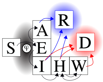
In the standard SEIR model, susceptible individuals $S$ become exposed $E$ (without symptoms), and after progressing to a symptomatic infectious state $I$, they become recovered $R$. Based on the available data, we extend the SEIR model with the states $(H,W,D)$, and regard them as worsened states of the symptomatic infection such that only a certain fraction of the infected individuals will enter them. It is widely accepted that not all exposed individuals become symptomatic [7] and hence we also extend the model by including an asymptomatic state $A$ with no or very mild symptoms.

The transmission is usually driven by random or time-dependent contact intensities between the susceptible and the infected individuals. As in [5, 52, 14, 51], we rather consider implicit spread via an infectious pressure compartment $\varphi$, an environmental state variable which models the current force of infection of the virus and which decays exponentially with time. Given that the decay rate of the infectious pressure is comparably fast and since direct spread can be understood as a timescale separation limit of indirect spread, most results should be robust with respect to this particular modeling choice (see also [6]).

The COVID-19 model in [34] sources the (explicit spread) infectivity from both symptomatic and asymptomatic carriers. We additionally allow for pre-symptomatic spread by sourcing the infectious pressure from all individuals in the states $(E,A,I)$. Originally, we intended for our framework to regularly simulate spread over a national network defined by commuting intensities between regions. However, in the end we did not routinely incorporate network spread in the model since with our available data, letting the regions function as independent nodes reduces the computational complexity while giving a very similar data fit.

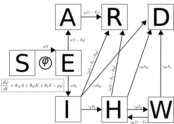
The resulting model is summarized schematically in Fig. 1, while a detailed description of the model and all parameters are found in the SI. With increased model complexity follows explanatory power at the expense of poorer model identifiability. With this in mind, we exclude all model refinements that are either missing or are unreliably or incompletely reported in the data, e.g., age and gender as well as certain refined states of minor symptoms. We recognize the infection’s varying effects on different age groups [17] and so must accept that our results remain in an age-averaged regime.

Figure 1: Proposed COVID-19 compartment model with indirect transmission. (S)usceptible contract the virus by exposure to an infectious pressure ($\varphi$), become (E)xposed and then enter either the (A)symptomatic or the (I)nfected state. Symptomatic severity follows: (I)nfected to (H)ospitalized to (W)orsen (intensive care), and to (D)eath. Only states A, I, and H can (R)ecover from the disease. The observables are H, W, and D. The infectious pressure is sourced from individuals in the states $(E,A,I)$ and decays exponentially with time.

Increased model complexity which, however, is required involves using a mix of dynamic and static parameters, since this allows the model to respond to functional changes such as societal interventions [27], vaccinations and virus mutations [39]. We thus let $\beta_{t}$, that is, the infection rate which is related to the reproduction number $R_{t}$, as well as the infection fatality rate (IFR) both be time-varying parameters. All in all the problem is then to determine the posterior distribution for 10 static and two dynamic parameters. The latter are assumed constant for periods of four weeks but are re-sampled independently for each such period.

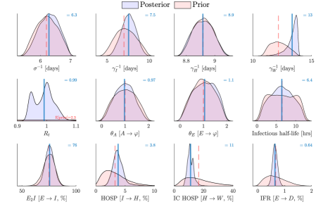
Clearly, well-chosen priors are required to make the problem definite. Considerable work went into constructing and continuously updating our priors using published research and public registries; the final priors are displayed in Fig. 2, with a complete list of priors and prior predictive estimates given in the SI.

Figure 2: Marginal priors (red) for the model parameters and the associated posterior distributions (blue) for the Swedish aggregate inferred from publicly available regional data from April 1, 2020 to May 30, 2021. The dashed lines indicate the prior means, and the full lines and numeric values the posterior means. Top row: latent period rate $\sigma$, and exit rates $\gamma_{X}$ out of compartment $X\in\{I,H,W\}$. Middle row: reproduction number and contribution to the infectious pressure $\varphi$ from compartments $A$ and $E$, respectively, as well as its decay (half-life). Bottom row: fractions proceeding between the indicated compartments. The reproduction number $R_{t}$ and the IFR are dynamic parameters and a temporal average is displayed here.

Approximate Likelihoods through Linear filtering

We understand the compartment model as a continuous-time Markov chain (CTMC) over an integer lattice counting the number of individuals in the different compartments. Hence the waiting time for exiting one compartment is exponentially distributed of mean rate $1/\lambda$, and the number of individuals which exit in a small window of time $[t,t+\Delta t)$ is Poissonian $\sim\text{Po}(n_{t}\lambda\Delta t)$, with $n_{t}$ the number of individuals at time $t$ in the compartment. If the number of individuals is large enough, this transition can be approximated by the normal distribution $\sim\mathcal{N}(n_{t}\lambda\Delta t,n_{t}\lambda\Delta t)$, which can be directly translated into a contribution to the state update matrices $(F_{k},Q_{k})$ of a discrete-time Kalman filter with the equations of state

$$x_{k+1} =F_{k}x_{k}+w_{k},\qquad w_{k}\sim\mathcal{N}(0,Q_{k}),$$ (1)

with $k$ the discrete time index corresponding to days.

The linear filter allows for an approximation of the intractable likelihood of a parameter proposal $\tilde{\Theta}$, namely the marginal filter likelihood,

$$p_{\tilde{\Theta}}(y) =\prod_{k=0}^{T}\mathcal{N}(y_{k}|H_{k}\hat{x}_{k|k-1},Q_{k}),$$ (2)

where $y_{k}$ is the data at time $k$, $H_{k}$ the observation matrix which maps the state to an observation, and where $\hat{x}_{k|k-1}$ is the Kalman state predictor at time $k$ given data until time $k-1$. In our application we rely on the likelihood to produce an approximate sample $(\Theta_{i})$ from the posterior using the Adaptive Metropolis (AM) algorithm [26]. The role of the marginal likelihood is remindful of a synthetic likelihood [54] and we refer to the specific combination of a Kalman marginal Likelihood and Adaptive Metropolis as KLAM.

Improved transmission rate estimation

The achievable temporal resolution of the Bayesian parameter estimates provided by Metropolis sampling is limited by both computational complexity and the amount of data. The procedure described so far yields static reproduction number estimates for each four-week period and with comparably large spread. To obtain more fine-grained estimates, a different approach is needed. Since the reproduction number is the dominating parameter of the dynamics, a more highly resolved estimate of the reproduction number is particularly useful. In terms of the parameters of the model, this corresponds to improving the estimation of $\beta_{t}$. Therefore, a daily estimate $\beta(t_{k})=\beta_{k}$ is calculated using dynamic optimization techniques.

Dynamic optimization has been used for estimating the reproduction number of the COVID-19 outbreak also by others [44]. When combined with an existing posterior distribution, care must be taken to avoid overconfidence from using the same data twice. For this reason, we do not attempt to derive an improved posterior distribution of $\beta_{t}$, but instead a single marginal time-dependent maximum likelihood estimate is sought, where the rest of the posterior distribution is “frozen” and consequently the parameter uncertainty is the same in absolute terms. The same logarithmic marginal likelihood that is used in the Kalman filter is utilized for this purpose, now understood as a quadratic cost function. Here, however, the deviation between measurements and the outputs from the mean-field dynamics is minimized, i.e., a shortened formulation compared to the filter is employed since the Kalman correction step is neglected. To avoid fast variations in $\beta_{k}$, a regularizing term penalizing square gradients is also added. The resulting optimization problem can be solved using standard techniques. Further details on the formulation of the optimization problem and its solution are provided in the SI.

Apart from providing more detailed information, this procedure yields improved confidence in the Bayesian workflow since it supports synthetic data with a known truth to be simulated in an off-line fashion. Our Bayesian inversion may thus be employed a second time in order to estimate bias or sensitivities for various estimates of interest, next to be described.

Assessing the quality of the approximate posterior

In real applications, a “true” or a “best” parameter posterior $\mathbf{P}^{*}$ is usually unknown. Evaluating the stability and the quality of the approximate posterior $\tilde{\mathbf{P}}$ is unfortunately often overlooked. We suggest employing a parametric bootstrap approach as in [14] to assess the error between samples from the true and the approximated posterior $\tilde{E}:=\tilde{\Theta}-\Theta^{*}$, where $\Theta^{*}\sim\mathbf{P}^{*}$ and $\tilde{\Theta}\sim\tilde{\mathbf{P}}$. Denote by $\theta^{*}:=\operatorname{\mathbb{E}}[\Theta^{*}]$, the minimum mean square error estimator (MMSE) of an assumed truth. Decomposing the mean square error around this value we find

$$\tilde{e}^{2} :=\operatorname{\mathbb{E}}[(\tilde{\Theta}-\theta^{*})^{2}]=\underbrace{\operatorname{\mathbb{E}}[(\tilde{\Theta}-\tilde{\theta})^{2}]}_{\text{Variance}}+\underbrace{(\tilde{\theta}-\theta^{*})^{2}}_{\text{Square bias}\,=:\,\tilde{b}^{2}},$$ (3)

where $\tilde{\theta}:=\operatorname{\mathbb{E}}[\tilde{\Theta}]$ is the MMSE of $\tilde{\Theta}$.

Formally, this still requires samples from the true posterior when estimating the bias. We approximate this via a bootstrapped estimator using a sample of $N_{\text{boot}}$ synthetic data sets generated from the MMSE of the approximate posterior. The generative simulator requires daily estimates of $(\beta_{k})$ or else the synthetic data quickly drifts off compared to the observations, and thus this technique ultimately hinges on the highly resolved marginal estimator described above. Posterior samples may then be generated for each synthetic set, yielding now a set of samples $\hat{\Theta}_{i}\sim\hat{\mathbf{P}}_{i}$, which allows for the use of the now tractable bias estimator $\hat{b}_{i}:=\operatorname{\mathbb{E}}[\hat{\Theta}_{i}]-\operatorname{\mathbb{E}}[\tilde{\Theta}]$. Our final estimator is then an average over these synthetic sets; $\tilde{b}^{2}\approx N_{\text{boot}}^{-1}\sum_{i}\hat{b}_{i}^{2}$ in (3). While up to $\numprint{196000}$ samples from each posterior were used to compute point estimators and credible intervals (CrIs), bootstrap replicas are much more costly to process so we used $N_{\text{boot}}=3$, and mainly relied on the bias estimator to diagnose non-robustness in point estimators. That is, a point estimator with CrI $A$ of order $\alpha=68\%$, say, and with bias estimate $\tilde{b}$ is considered less robust whenever

$$\tilde{b}\geq 0.5\operatorname{\mbox{diam}}(A).$$ (4)

The bootstrap posterior densities can be used in aggregate form for bias estimation and check of estimator robustness as just described, or for a related check of credible interval robustness. Consider two CrI intervals $A$ and $B$ of order $\alpha$, e.g., $\alpha=68\%$, and where $B$ is a bootstrap replicate of $A$. A basic measure of the robustness of $A$ is the level of overlap between $A$ and $B$ and one can reasonably require the same overlap as the indicated order $\alpha$, i.e., to require

$$\operatorname{\mbox{diam}}(A\cap B)\geq\alpha\operatorname{\mbox{diam}}(A\cup B).$$ (5)

If this criterion is satisfied, then a random variable drawn uniformly from $A\cup B$ has probability $\geq\alpha$ to also be in $A\cap B$. The robustness checks Eqs. (4)–(5) are explicitly reported in Tab. 2, but were also routinely employed when evaluating various results.

Results

Our model was used for weekly reported predictions within CRUSH Covid. Prior to each report we carried out a model updating procedure: new data were pulled from public repositories and screened for contradictory or incorrect values. The posterior was sampled by KLAM using an initialization either from an estimated initial state as described in the SI and developed for this very purpose, or simply using stored state samples. The latter allows for faster sampling as it reduces the burn-in period: about 24 hours of compute for 21 regions and a year’s worth of data on a 4-core laptop was then reduced to a few hours. The final posterior model was queried for one-week-ahead forecasts with uncertainty bounds for the $(H,W,D)$ triple. We also continuously evaluated the previous week’s predictions against the up-to-date data in the same round.

Posterior prediction

In Fig. 2, we display the prior distributions together with the resulting Swedish aggregate posterior, i.e., the population weighted average of the individual posterior of each of Sweden’s 21 regions. Several priors are clearly very similar to their respective posteriors, e.g., the latent period rate $\sigma$ and the symptomatic period rate $\gamma_{I}$. This is expected and simply indicates little information in the observations for these parameters relative to the prior. Our data also cannot improve on the prior for the share of spread from exposed (pre-symptomatic) and asymptomatic individuals (parameters $\theta_{E}$ and $\theta_{A}$, respectively). This is simply due to the fact that we have no continuously reported data neither for $E$ nor for $A$. On the same note we had to rely on a directed study [7] to define the prior for the parameter $E_{2}I$, i.e., the fraction of exposed individuals who eventually develop symptoms.

Of more interest are the parameters that govern the fraction that transition to a worsened state of the disease: $I\rightarrow H$ and $H\rightarrow W$. Our results show that $3.8\%\,[2.2,5.9]$ (95% Credible Interval (CrI)) of the symptomatic individuals require hospital care, and $11.2\%\,[7.6,16.1]$ of the hospitalized patients require intensive care. During the considered period, the Swedish Public Health Agency (PHA) published five point estimates of those same fractions. The relevant demographic average of these are $I\rightarrow H$: $3.0\%\,(2.4,3.6)$ and $H\rightarrow W$: $14.3\%\,(9.8,18.8)$ (mean $\pm\,2$ std, $n=5$) respectively [17]. Additionally, [46] found similar estimates in France $I\rightarrow H$: $2.9\%\,[1.7,4.8]$ and $H\rightarrow W$: $19.0\%\,[18.7,19.4]$. We could have used the earlier of those point estimates to improve on the corresponding priors, however, as validation possibilities are scarce, we decided to rather use them for this purpose instead.

Figure 3: Seven-day ahead prediction in the Uppsala region. Shaded area shows 68% CrI, and the points are the observations. The dotted vertical lines indicate the four-week periods used for the dynamic rates.

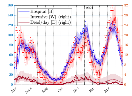
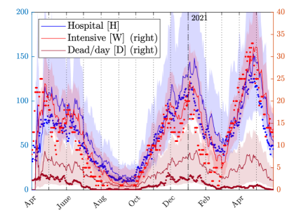
The regional models were used for posterior predictions on a weekly basis, e.g., one 7-day ahead prediction for the Uppsala and Stockholm regions, respectively, and one in aggregate for the entire nation. In Fig. 3 this is exemplified over a longer period together with the actual outcome. The performance of the weekly predictions which were reported live ($N=25$) is presented in Tab. 1. Each prediction included a mean with 68/95% CrI. The week after publishing, we evaluated the prediction against the then-available data. The predictions performed better in the medium sized region Uppsala and notably, the predictions for casualties were poor in the larger region Stockholm. The observed misfit in casualties eventually lead us to reconsider the role of the IFR parameter, initially just a static parameter, and we decided to let it be dynamic as described previously. In the live reporting in Tab. 1, only 9 of the 25 reports allowed for a dynamic IFR. Another possible reason for the poorer prediction performance in the Stockholm region could be that, since this region contains three large hospitals, the greater heterogeneity in terms of reporting makes identification more challenging. One can rightly question if smaller sub-regions should rather be modeled here, but we did not have access to the data to drive such a model.

In the SI we further compare the quality of the Kalman predictor with that of a simpler regression-based estimator. The latter provides accurate mean-square predictions and is very fast to evaluate. The overall advantage with our approach lies rather in that the Bayesian posterior model itself can be investigated for further epidemiological insight, next to be discussed.

	Hospital (H)	Intensive (W)	Death (D)
Uppsala (68%)	76	72	68
Stockholm	64	64	36
Sweden	88	44	32
Uppsala (95%)	100	100	96
Stockholm	84	92	68
Sweden	96	92	68

Table 1: Frequency (%) of all weekly reported predictions that fell inside of (68/95% CrI, 7 days ahead), evaluated on the following week (N = 25). Note that the Uppsala results are very close to the ideal 68/95% outcome.

Posterior hidden state estimation

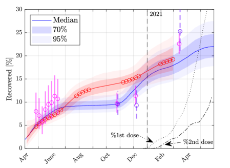
The posterior model can also be used as a kind of “Bayesian twin” and estimate quantities that are otherwise very difficult to approach. For example, we can readily estimate the number of individuals that have contracted the disease and survived; these individuals are the ones that could potentially have developed antibodies that are detectable in serology tests. In Fig. 4, we visualize several reported results for Stockholm [8, 18] and our estimates. Those estimates compare very well, and notably so given that no screening data was used by our method.

Figure 4: The fraction of recovered individuals in the Stockholm region. Our model (blue), is set to 2.35% on April 5, 2020 (matching [8]). Serology-based Bayesian model predictions [8] (red) which reported 70/95% CrIs. Estimated mean prevalence of antibodies found in spared blood samples from outpatient care, with 95% CI (solid, pink) and blood donors (dashed, purple) [18]. On 2020, December 27, the Swedish vaccination campaign started and both the number of delivered first doses (dotted) and second doses (dash-dot) are indicated.

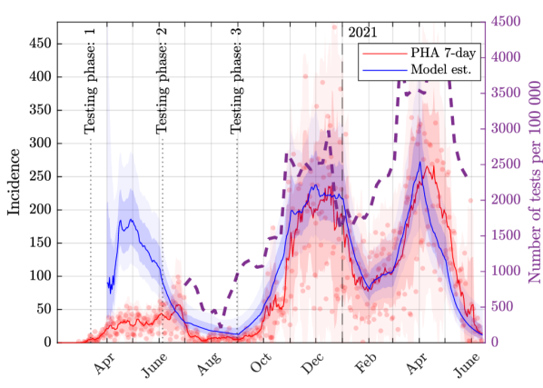
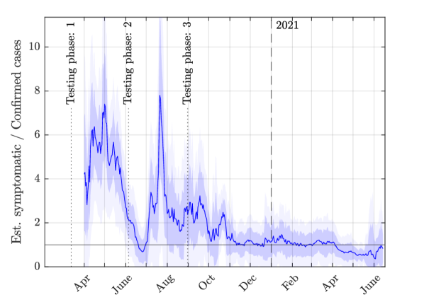
The posterior model can also estimate the symptomatic incidence in the same vein. Fig. 5 illustrates our estimated symptomatic incidence and the reported number of positive RT-PCR tests by the PHA for Uppsala. As testing increases, the ratio between our estimate and the positive tests oscillates around one, indicating that the testing at that time captures most of the symptomatic infected.

These two examples demonstrate that our computational model can be used to effectively estimate hidden variables at the same regional resolution as supported by data. The financial cost for this kind of monitoring would of course be a tiny fraction compared to any alternatives based on testing.

Figure 5: Left: the estimated symptomatic incidence from our model (blue with [68,95]% CrIs shaded) and the confirmed cases by PHA (red line 7-day smoothed and uncertainty from rolling $\pm[1,2]$ standard deviations shaded, with data as points) for Uppsala. The right axis gives the number of tests per 100 000 inhabitants per week (dashed). The total number of tests administered during Testing phase 3 was approximately 360 000. The dotted vertical lines mark the boundaries of testing phases as defined by policy changes affecting the testing volumes. Right: the ratio between the model’s symptomatic incidence and the confirmed cases incidence indicates the proportion of cases that are missed by testing. Values above one thus hint at an underreporting of symptomatic cases.

Marginal risks

Recall that the IFR is defined as the proportion of deaths among infected individuals, i.e., including asymptotic cases. By design, our model relies on an IFR which is constant over four weeks. Our estimated IFR for Sweden stayed relatively constant over the period May 2020–November 2020 at $0.69\%\,[0.11,1.5]$ (95% CrI). For comparison, in April 2020, the PHA published an early estimate of $0.58\%\,(0.37,1.05)$ (95% CI) for Stockholm, Sweden [16]. However, this estimate relies on initial assumptions on the number of undetected cases that seem unjustified when compared to later findings [42, 31]. It also assumes the relatively younger Stockholm demographics rather than the national one, and is therefore an underestimate of the national IFR. A later Sweden-wide IFR estimate of $0.76\%\,[0.65,0.87]$ was published in November 2020 [22] and aligns well with our estimate above. Although our 95% CrI is comparatively wide, this is partially due to modeling each period independently and without any regularization in the transition between periods.

Tab. 2 summarizes a few bi-monthly estimates for the period after October 2020. The first two entries in the table overlap the estimates from [9]: Nov 2020 $=[0.60,1.46]\%$, and Jan 2021 $=[0.56,1.44]\%$. Clearly, the IFR was trending downwards and this is also known to be the case in Stockholm [22] as well as for the world in general [9].

	Stockholm	Uppsala	Sweden
Oct+Nov	0.66 [0.34, 0.81]	0.49 [0.24, 0.74]	0.55 [0.27, 0.88]
Dec+Jan	0.84 [0.71, 1.00]	0.59 [0.28, 0.92]	0.88 [0.55, 1.30]
Feb+Mar	0.35 [0.18, 0.50]	0.47 [0.23, 0.70]	0.44 [0.22, 0.81]
Apr+May	0.35 [0.19, 0.49]	0.45 [0.22, 0.67]	0.35 [0.18, 0.56]

The estimated bias is large compared to the 68% CrI (see Material and Methods).

The 68% CrIs of the posterior and the bootstrap replicate do not share at least a 68% overlap (see Material and Methods).

Table 2: Bi-monthly estimated IFR [%] with 68% CrI from October 2020 to May 2021.

Of interest is also the case fatality risk (CFR) [35], i.e., the risk of death conditioned on being diagnosed with the disease. We more generally define CFR_X as the proportion of deaths expected given a certain number of individuals in compartment $X\in\{I,H,W\}$. Note that CFR_I involves the number of symptomatic individuals which formally is not the same thing as the number of cases confirmed by testing.

From our posterior we may directly estimate the national average CFRs to be $\{\text{[\ltx@text@number{0{.}72},\,\ltx@text@number{1{.}3}]},\text{[\ltx@text@number{16},\,\ltx@text@number{19}]},\text{[\ltx@text@number{34},\,\ltx@text@number{36}]}\}\%$ (95% CrIs) for CFR_I, CFR_H, and CFR_W. By comparison, [2] offers the estimates CFR_I $=(1.0,3.0)\%$, CFR_H $=(9.0,17.0)\%$, and CFR_W $=(24.0,51.0)\%$ (95% CI).

Another way to investigate these risks is by running the posterior filter across our data to produce an estimate for the number of deceased per compartment. Until March 23, 2021 we find for all of Sweden that $\{D_{I},D_{H},D_{W}\}=\{\text{[\ltx@text@number{1{\,}786},\,\ltx@text@number{8{\,}652}]},\text{[\ltx@text@number{3{\,}612},\,\ltx@text@number{8{\,}096}]},\text{[\ltx@text@number{1{\,}126},\,\ltx@text@number{3{\,}627}]}\}$ (95% CrIs). From NBHW data we may estimate those same numbers to be $\{\numprint{8335},\numprint{4102},\numprint{935}\}$ [48], after a scaling of about 5% to arrive at the same total number of dead as in our dataset ($D=\numprint{13372}$). Apparently, our model overestimates the deaths under ICU and to some extent also at hospital, while our estimate for deaths outside hospital is underestimated compared to this data point. This could likely improve given more detailed data sources, including, e.g., improved records of COVID-related deaths and hospital care outcomes.

Reproduction number estimates

The reproduction number provides an essential insight into the future development of the spread of a disease in a population. An accurate estimate of this number is vital to support rational public health decision-making and to inform the general public. Temporal variations in the reproduction number are caused by socio-behavioral, environmental, and virological and biological factors [11]. The dynamics of the reproduction number is therefore significantly faster than those of most other parameters, which was also the motivation behind our development of an improved marginal estimator via dynamic optimization techniques as described previously.

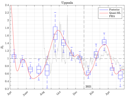
Reproduction number estimates have been calculated in this way for the whole duration of the parameterized period for all regions in Sweden. In Fig. 6, we present our results for Uppsala together with the testing-based estimate produced by the PHA for the same period. The cost-effectiveness of our estimate is apparent here since the results are similar, but the PHA estimate relies on costly incidence data.

Figure 6: Reproduction number estimates for the Uppsala region. The Bayesian posterior yields monthly estimates (box-plot) while the quasi-ML estimator is daily (solid). For comparison also the PHA’s estimates based on screening from of a total of 367 200 RT-PCR tests during the period 5 August, 2020–May 26, 2021. Note that reproduction numbers are model specific and the comparison here is therefore mainly qualitative.

Discussion

The pathogen SARS-CoV-19 and the subsequent pandemic resulted in an explosion in research related to COVID-19: research on data collection and interpretation, modeling and forecasting, as well as scenario generation. From the beginning of the outbreak, data have been instrumental in understanding the disease dynamics [38, 37, 55]. With increasing amounts of cases and recorded patient data, statistical models for diagnosis and prognosis were quickly developed [57]. Combining in-patient data with other covariates, the use of digital technologies for disease surveillance is now possible [1], notably with an impact also for COVID-19 [40, 12, 43, 36]. Challenges connected to the collection and distribution of available data where met with specialized tools for decentralized publishing [25, 41] and anonymized mobility data were also in active use [30, 29].

We have devised a detailed Bayesian model for the regional dynamics of the COVID-19 pandemic in Sweden. A data-centric viewpoint is that, using model-based data analysis, we have gained a thorough insight into the progression of the COVID-19 pandemic in Sweden in general, with extra emphasis on the Uppsala Region. The proposed compartment-based model combined with the novel use of optimal linear filters turned out to be an effective information-theoretic epidemiological tool. The output quality as obtained in our work compares very well with official estimates gathered in test-based programs, cf. Figs. 4–6. During the second and third waves in Sweden, at least 10 million RT-PCR tests were administered at a standard cost of 1 400 SEK ($\approx\$150$) per test [50]. The expenses for such a PCR test for all symptomatic-strategy quickly grows, underlining the economical advantages of our approach. Clearly, at the individual level there are several benefits with testing and the importance of screening as a means to collect initial statistics for the disease spread cannot be stressed enough. However, our approach remains very promising as a supporting tool to continue to monitor the situation when testing is limited due to risk-cost trade-offs.

The resulting model was further processed to output weekly predictions for health care demands, and also marginal estimators for important characteristics of the disease such as infection fatality rates and reproduction numbers. The latter output increased the confidence into the overall approach through the generation of synthetic data and parametric bootstrap techniques. Improved data that would have enabled a higher model precision include (1) a consistently managed incidence report from randomized testing (not necessarily high volume), and (2) a higher temporal resolution of hospitalization and intensive care risks as well as times for treatment in these respective categories. These statistics could both be collected at a relatively small cost but would likely improve the precision considerably.

Without relying on public testing strategies, our model-based approach provided improved situation awareness of the progression of the pandemic. The developed methodology is of highly general character and can therefore be expected to be useful in other contexts too. By virtue of the consistent Bayesian framework, uncertainties are transparently propagated under clear assumptions, also in the face of potentially hazardous situations. We argue that this quality makes the techniques developed herein particularly promising from a communicative perspective.

Our data streams are high in latency, but are on the other hand fairly low in noise. Low-latency signals, e.g., public screening, self-reporting mobile apps, or analysis of sewage water, are instead often more noisy or otherwise biased. Combining these different kinds of streams provides for excellent decision support and appears extremely promising for use in tracking regional epidemics at a near-daily resolution.

Acknowledgments

This work was financially supported by the Swedish Innovation Agency Vinnova, by the Swedish Research Council Formas (S. Engblom), and by the Swedish Research Council (H. Runvik and A. Medvedev).

Author contributions

SE conceived the research and RM and SE developed the initial forward model. Linear filters were designed by SE and HR who also developed and operated the dynamic optimization approach with inputs from AM. SE developed priors and data pre-processing and RM adapted the Bayesian sampling techniques, collected data, performed computations, and prepared the manuscript joint with SE and with inputs from HR. All authors took part in revising the manuscript.

Supporting Information:
Bayesian Monitoring of COVID-19 in Sweden

This supplement contains further explanations and details of the data, the model, and the computational methodology, as well as some additional results mentioned in the main article. The SI is organized in sections as follows:

Additional supporting results

• Incidence: our model’s estimate of the incidence of symptomatic cases compared to the number of confirmed cases by PHA in Stockholm (complementing the Uppsala cases in the main article). This also produces an estimate of the proportion of undetected symptomatic cases.

• $R_{t}$-estimators: for a selection of small and large regions.

Data

A summary of the various sources and use of data.

Compartment model

Our extended SEIR-model in detail, including an explanation of all model parameters.

Priors

The parameter priors for the model and how they were determined.

Kalman filter

The linear filter approximation of the continuous-time Markov chain, which in turn is our probabilistic understanding of the extended SEIR-model.

Posterior sampling

Details of the Metropolis sampling procedure.

Dynamic optimization solution

The procedure for ‘bootstrap on the margin’ to improve the temporal resolution of the reproduction number estimator.

Additional evaluations

• Posterior robustness: A comparison of the 21 regional posteriors, which thus form a natural bootstrap population.

• Bootstrap robustness: The estimated bias and some additional quality statistics for the 21 regional posteriors.

• Baseline predictor: A comparison of the prediction of our Kalman filter and a simpler regression estimator.

Reproducibility

The code as well as the data required for reproducing the results in the paper are publicly available and can be downloaded at github.com/robineriksson/Bayesian-Monitoring-of-COVID-19-in-Sweden. Refer to the included file README.md for more information.

Additional supporting results

Incidence estimates: a comparison between model- and test-based results

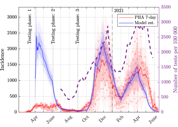
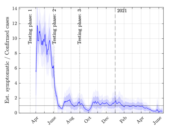
In the main paper, we illustrate how the posterior model can estimate the incidence of symptomatic cases, which is a hidden state and thus does not correspond directly to data. Here we display the corresponding estimates for Stockholm, see Fig. 7. The reported tests are smoothed by a 7-day Savitzky-Golay filter and the estimated uncertainty is the corresponding rolling standard deviation. After testing phase 3, the ratio between our estimate and the positive tests oscillates around one, indicating that the testing at that time captures most of the symptomatic infected. After April 2021, our model estimates a somewhat smaller symptomatic incidence than what was captured in actual tests. A possible explanation for this is that at smaller incidence, an increasing proportion of asymptomatic cases are included in the test pool, e.g., from regular screening of hospital personnel and similar.

Through this method of exploring the data we can also confirm our early suspicion that the incidence data signal was poor during Testing phase 1 and in part during phase 2. The noise in the screening data explains the nervous behavior of the PHAs reproduction number estimates as seen in Figs. 6 and 8. At the start of the second wave, and during Testing phase 3, this signal was much more accurate albeit at huge economical costs.

Figure 7: Left: the estimated symptomatic incidence from our model (blue with [68,95]% CrIs shaded) and the confirmed cases by PHA (red line 7-day smoothed and uncertainty from rolling $\pm[1,2]$ standard deviations shaded, with data as points) for Stockholm. The right axis gives the number of tests per 100 000 inhabitants per week (dashed). The total number of tests administered during Testing phase 3 was approximately 1 800 000 for Stockholm. The dotted vertical lines mark the start of new testing phases that are defined by policy changes affecting the testing volumes. Right: the ratio between the model’s symptomatic incidence and the confirmed cases incidence indicates the proportion of cases that are missed by testing.

$R_{t}$-estimators

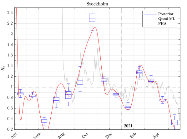
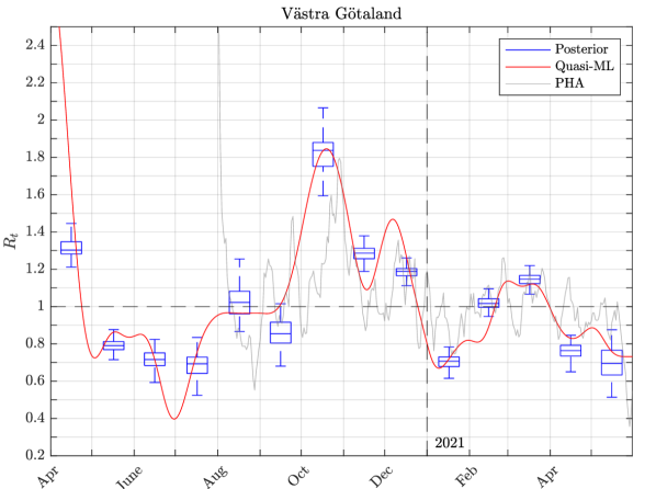
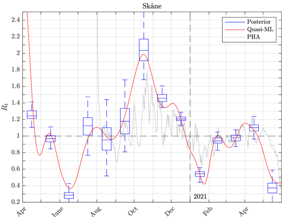
We illustrate the daily $R_{t}$-estimators for the three largest and the three smallest (by population) regions: Stockholm, Västra Götaland, Skåne (largest), and, respectively, Gotland, Jämtland, and Blekinge (smallest) in Fig. 8. The relative uncertainty is visibly smaller in the larger regions than in the smaller ones, a typical small population effect as the data streams for the smaller regions consist of smaller counts with larger uncertainties in a relative sense.

Figure 8: Our daily reproduction number estimate (in red, with box plots for each 4-week constant posterior) and the publicly reported PHA estimates from the Swedish screening program (in grey). The three largest regions are: Stockholm (top left) [1 864 000 total # of RT-PCR tests administered during the 2nd and 3rd waves, August 5, 2020–May 26, 2021], Västra Götaland (top center) [1 570 000], and Skåne (top right) [1 240 000], followed by the estimate for the three smallest regions: Gotland (bottom left) [48 440], Blekinge (bottom center) [110 300], and Jämtland (bottom right) [184 300]. The standard cost per PCR test was 1 400 SEK ($\approx\$150$) [50].

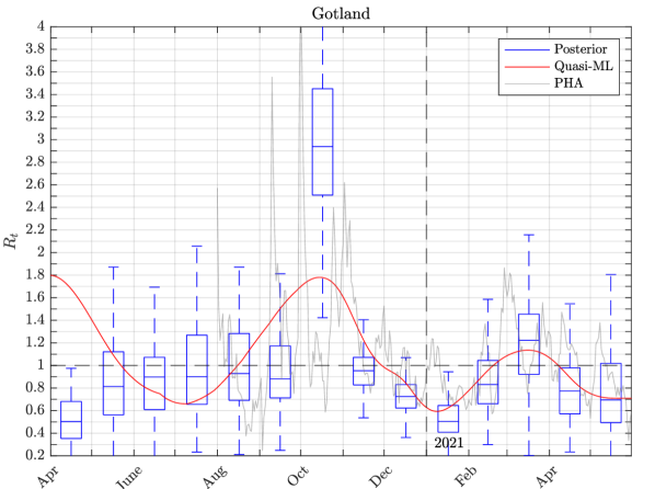
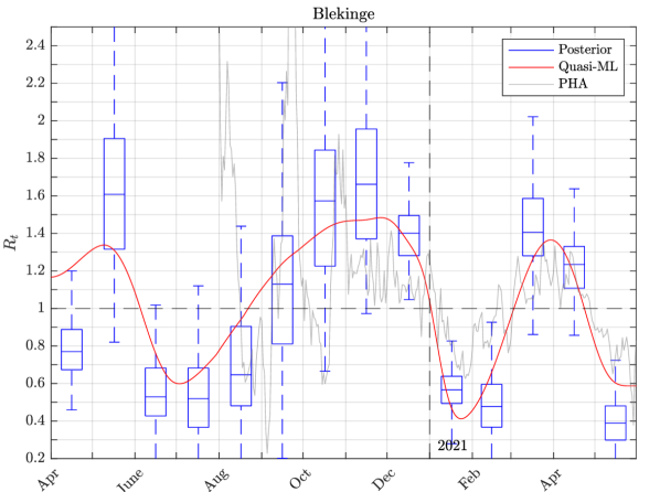
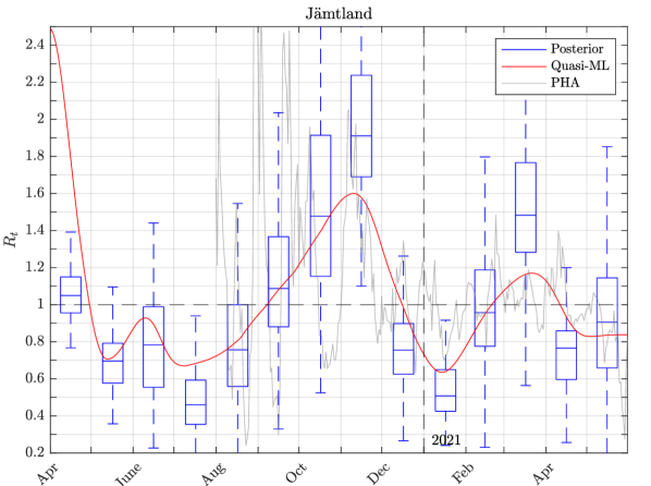
Data

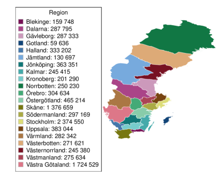
The daily observations we use in the inference is retrieved from c19.se using Python scripts. In turn, c19.se fetches the data from the official regional sources on a daily basis. Sweden has 21 regions (Fig. 9) that are in charge of providing for the healthcare of its population. They also present data on the number of hospitalized patients, the number of patients in intensive care, and the daily number of diseased by COVID-19. We use a couple of other datasets for prior generation and for posterior validation, see Tab. 3. The sets C19 and NBHW_D had double use, however, the prior information obtained from these were on an aggregated level.

Name	Description	Time-series	Regional	Use	Source
C19	Collection of regional reports $(H,W,D)$	Yes	Yes	Prior, Inference	[data2020c19]
PHA	Incidence of confirmed cases $(I_{\text{inc}})$	Yes	Yes	Validation	[data2020fhm]
NBHWD	Total # of deaths $(D_{I},D_{H},D_{W})$	No	No	Prior, Validation	[48]
NBHWγ	Recovery times at hospital and ICU	No	No	Prior	[ss2020vard]
SIRD	# of deaths as ICU $(D_{W})$	Yes	Yes	Prior	[sir2020mort]
FHM${}_{R_{t}}$	Estimated $R_{t}$ per region from $I_{\text{inc}}$	Yes	Yes	Validation	[rtal2021fhm]
FHM${}_{Rec}^{1}$	PHA seroprevalence study, outpatient care	No	No	Validation	[18]
FHM${}_{Rec}^{2}$	PHA seroprevalence study, blood donors	No	No	Validation	[18]
CastroR	Estimated Recovered in Stockholm	Yes	No	Validation	[8]
SCB${}_{\text{trans}}$	Regional in-/out commuting	No	No	Prior	[pend2019scb]

Table 3: Summary of data sources used for prior, for inference, and for validation.

Figure 9: Sweden is divided into 21 regions. We find a posterior distribution for each of the individual regions as each region publish their own data of observables. In the legend the population size of each region is given (as of December 9, 2019 [data2020scb]), which spans from the smallest: Gotland (59 636), to the largest: Stockholm (2 374 550).

Data pre-processing

Our main data sources were updated each day and incorrect or questionable data points were common. Two errors that need to be addressed are next described. First, there are impossible or very extreme updates, e.g., a negative incidence or very large jumps, most likely due to an accumulation of delayed reports, or in some cases possibly in an attempt to correct earlier reports. For example, a delay in the reporting of deceased has been described in the Swedish data set [4], and was there explained as “batch” reporting. In similar spirit, there are also a few missing data points. However, these are all found very early on in the data history and could safely be replaced with NaN-values, thus simply ignored. Second, and more problematic from a model-based perspective, is the fact that parts of the reporting display a strong periodic component, which is not supported by the model and rather most likely an effect of weekday periodicity.

The pre-processing of data is done in two steps. First, we ensure that there is no negative incidence data. Negative values are detected and set to 0, with values backwards in time corrected in a ‘reasonable’ way using a simple linear decaying memory kernel, and with the corresponding cumulative compartment adjusted accordingly. In this first step we also replace missing or manually found early outlier measurements with either linearly interpolated data from adjacent days, or using NaN-values. The second step involves smoothing the cumulative fields and the incidence fields to mitigate the effects of weekly periodic lags or batch reporting. The smoothing algorithm removes unlikely incidences by starting from the most extreme outliers, e.g., $\geq[10,9,\ldots,2]$ standard deviations under a Poissonian approximation, and spreads them out during the period before in such a way as to dampen weekday dependencies in reporting. 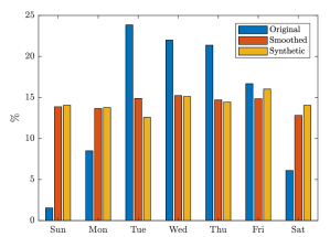Most weekly periodicity is removed by this procedure, see Fig. 10 for an example, and whatever remains does not seem to interfere with the Bayesian inference. The total effect the pre-processing has on the data can be measured in the sense of the mean maximum relative difference,

$$d_{\text{smooth}} =N_{t}^{-1}\sum_{t}\max_{i}\frac{|X^{(i)}_{\text{smooth}}-X^{(i)}|(t)}{\max(1,|X^{(i)}(t)|)},$$ (6)

where $i\in\{1,2,3\}$ for compartment $X\in[H,W,D]$, i.e., the three data compartments and over some period of time of length $N_{t}$. We report this measure for the period April 1, 2000–May 31, 2021 in Tab. 6. The population weighted national average difference is $6.6\%$.

Figure 10: Reports of deceased per weekday over the period April 1, 2020–May 31, 2021 for the Stockholm region. The smoothing procedure attempts to correct for weekly reporting patterns in the original data and behaves similarly to a bootstrap replicate for the same time period and region.

Compartment model

The extended SEIR model is depicted in Fig. 11. The transitions in the figure are modeled via transition rates corresponding to exponentially distributed waiting times in a continuous-time Markov chain interpretation.

The compartment model we consider stems from the SIS${}_{\text{E}}$-model [5](Chap. 11). This model contains three state variables, $[S,I,\varphi]$. The first two are integer compartments and are defined by the Markovian transitions

$$S \xrightarrow{\beta\varphi\Sigma^{-1}}I,\qquad I\xrightarrow{\gamma}S,$$ (7)

with $\Sigma=S+I$, the total population size. Susceptible individuals turn infected at a rate proportional to the local infectious pressure $\varphi$, and infected individuals recover at a rate $\gamma$. The last compartment $\varphi$ represents the environmental pathogen load and follows the dynamics [siminf_Ch]

$$\varphi^{\prime}(t) =\theta_{I}I(t)-\rho\varphi(t).$$ (8)

Infected individuals shed the pathogen into the environment, thus sourcing the infectious pressure, which also decays at a fixed rate $\rho$.

The $R_{0}$-number for the SIS${}_{\text{E}}$-model is given by $R_{0}=\theta_{I}\beta/(\gamma\rho)$ provided that $\varphi$ is not considered a state-at-infection [Diekmann2010], or alternatively, $R_{0}^{(\varphi)}=\sqrt{R_{0}}$ if this interpretation is more natural, e.g., for vector-borne diseases [51]. In either case $\theta_{I}=\rho$ is a convenient non-dimensionalization.

Our extended SEIR-model involves two types of parameters: rates and fractions. The rates are $[\beta_{t}$, $\sigma$, $\gamma_{I}$, $\gamma_{A}$, $\gamma_{H}$, $\gamma_{W}$, $\theta_{A}$, $\theta_{E}$, $\theta_{I}$,$\rho]$, and the fractions $[F_{0}$, $F_{1}$, $F_{2}$, $F_{2d}$, $F_{3}$, $F_{3d}$, $F_{4}]$. We may further divide the rates into waiting times and those governing the infectious pressure. The waiting times are $\sigma$, $\gamma_{I}$, $\gamma_{A}$, $\gamma_{H}$, and $\gamma_{W}$, and are understood as the inverse of the mean time an individual stays in a certain compartment, e.g., the mean recovery time for a symptomatic infected is $\gamma_{I}^{-1}$. The transition from $S$ to $E$ depends on $\varphi$ and $\beta_{t}$. The infectious pressure $\varphi$ is sourced by the viral shedding from asymptomatic $\theta_{A}$, from exposed $\theta_{E}$, and from symptomatic individuals $\theta_{I}$, and it decreases by the viral decay rate $\rho$. We use the non-dimensionalization $\theta_{I}=\rho$ and the scaled variables $\theta_{E}=\theta_{E^{*}}\times\rho$ and $\theta_{A}=\theta_{A^{*}}\times\rho$.

For this model the reproduction number can be determined using the next generation method, and under the interpretation that $\varphi$ is not a state-at-infection [Diekmann2010],

$$R_{0}=\beta_{0}\bigg{(}\frac{\theta_{E^{*}}}{\sigma}+\frac{(1-F_{0})\theta_{A^{*}}}{\gamma_{A}}+\frac{F_{0}+(1-F_{0})F_{1}}{\gamma_{I}}\bigg{)},$$ (9)

and an identical relation holds for $(R_{t},\beta_{t})$. As with the SIS${}_{\text{E}}$-model, we have that

$$R_{0}^{(\varphi)}=\sqrt{R_{0}}$$ (10)

if instead, $\varphi$ is understood as a state-at-infection.

The fraction parameters determine the probabilistic fates of individuals in a compartment with more than one exit. They were determined from demographic averages since the daily data did not contain the level of detail to support age-dependency (cf. the discussion in Material and Methods).

$$E\rightarrow I: \quad F_{0}=E_{2}I,$$ (11)

$$A\rightarrow I: \quad F_{1}=A_{2}I\quad(=0\,\text{ in our simulations}),$$ (12)

$$I\rightarrow H: \quad F_{2}=\text{HOSP},$$ (13)

$$H\rightarrow W: \quad F_{3}=\text{IC\leavevmode\nobreak\ HOSP},$$ (14)

$$H\rightarrow D: \quad F_{3d}=\text{SIR MORT }\times\text{ HOSP MORT},$$ (15)

$$W\rightarrow D: \quad F_{4}=\text{SIR MORT},\quad\mbox{ and,}$$ (16)

$$I\rightarrow D: \quad F_{2d}=\max\left(0,\frac{\text{IFR}}{E_{2}I}-\frac{(\text{HOSP MORT}+\text{IC\leavevmode\nobreak\ HOSP})\times\text{SIR MORT}\times\text{HOSP}}{1-\text{IC\leavevmode\nobreak\ HOSP}\times(1-\text{SIR MORT})}\right).$$ (17)

The final relation is best explained from the discussion leading to (25) below. The remaining fractions of the model can generally be obtained by requiring that the total sum of all outgoing fractions is one. That is, the fraction which recovers from compartment $X$ is given by $1-F_{X}-F_{Xd}$, where $F_{X}$ is the fraction that enters the next state in the chain and where $F_{Xd}$ is the fraction that dies.

Note that the model parameters covering fatalities, $(F_{2d},F_{3d},F_{4})$, are obtained from the more natural parameters $(\text{SIR MORT},\text{HOSP MORT},\text{IFR})$ via Eqs. (15)–(17).

Figure 11: Detailed compartment model of Fig. 1 with related transition rates. The dashed arrow indicates the interaction with the environmental compartment $\varphi$.

Network effect for national scale simulations

We did not find that connecting the regions improved the fit to data and, in the end, we therefore decided not to use this technique on a regular basis. However, since we did use it in Tab. 1 and for completeness, we describe below how it was implemented.

The network connection is obtained by introducing a prior commuting intensity factor $\lambda$ that allows for connections between the regions. This affects only the calculations on a national level, and it does so mainly by adding some correlation between connected regions.

The network is defined by a connection matrix $D$ which is a 21-by-21 square matrix with a zero diagonal. For the $i$th row, each column $j$ contains the proportion of individuals commuting into region $i$ from region $j$. In turn, the connection matrix itself is found by a linear programming formulation on the volumes of individuals commuting in and out per each region [pend2019scb]. At each forward step in the simulation, the infectious pressure $\varphi_{k}=\varphi(t_{k})$ is then updated as

$$\varphi_{k+1} =\bar{\varphi}_{k+1}+\lambda(D\varphi_{k}-d\odot\varphi_{k}),$$ (18)

where $\bar{\varphi}_{k+1}$ is the update according to Eqs. (29)–(31), i.e., without any network effects, and where $d$ is the column sum of $D$ and $\odot$ is element-wise multiplication.

Priors

The prior knowledge relied upon to construct priors stems from several sources. Below we briefly comment on the techniques and assumptions used to derive our priors; effective summaries are found in Tabs. 4 and 5. The process of constructing priors was ongoing during the whole period fall 2020 to late spring 2021. We revised the priors whenever we became aware of new research, when more statistics became available, or we deemed model tweaks necessary. The final priors (arrived at towards the end of May 2021) are what we discuss below.

$\boldsymbol{\sigma}$ and $\boldsymbol{\gamma_{I}}/\boldsymbol{\gamma_{A}}$

The mean incubation time $\sigma^{-1}$ is set to $6.2$ days with support in $[5.4,7]$, derived from the mean and 95% CI given in [dhouib2021incubation]. The recovery time for the symptomatic infectious $\gamma_{I}^{-1}$ is less known and we therefore set the mean to $7$ days [7][ferretti2020quantifying] with a wider support of $[4,10]$ days. We assume similarity between asymptomatic and symptomatic cases by setting $\gamma_{A}=\gamma_{I}$, which covers the priors suggested in [7].

$\boldsymbol{\gamma_{H}}$ and $\boldsymbol{\gamma_{W}}$

We determine the priors for hospital recovery times, $\gamma_{H}^{-1}$ and $\gamma_{W}^{-1}$ from a dataset published by the NBHW [ss2020vard], including the distribution of exit times for hospital patients with and without ICU care. The dataset is right-tailed censored for waiting times over 30 days, which affects the ICU patient records. For $\gamma_{H}^{-1}$, we first make a Bayesian fit of an exponential distribution to hospital caring time data ($N=\numprint{40507}$ patients) and place a somewhat broader beta distribution across the credible interval for the hyper parameter thus found, this results in a beta distribution of mean $8.9$ and support on $[8.7,9.1]$ [days]. The recovery time under intensive care, $\gamma_{W}^{-1}$, is more complicated since the available data involves also non-ICU caring times. Assuming the previously determined exponentially distributed waiting times under hospital care, we first subtracted two such waiting times (to model pre- and post-ICU care, respectively), next made a Bayesian exponential fit to the remaining time ($N=\numprint{4039}$ patients). This fit was judged a bit worse than for non-ICU care time and so we used a larger enclosing support of $[10.8,13.9]$ with mean $12.2$ [days].

$\boldsymbol{E_{2}I}$

The prior for the fraction $E_{2}I\,(E\rightarrow I)$ was taken from [alene2021magnitude]: $0.75\,(0.62,0.84)$ (95% CI), for which we determine a scaled beta distribution that fits the mean and the given CI interval. The resulting prior distribution has mean $0.75$ and support on $[0.014,1]$.

IFR

The IFR, i.e., the eventual fraction of infected individuals that dies ($E\rightarrow D$ in our model), is volatile in that the IFR depends strongly on the age distribution of the region as well as on the quality of the health care and the currently dominating virus variant [brazeau2020report, 16]. We therefore settled on a scaled beta distribution with positive skewed and rather wide support: $0.67\%,[0,2]\%$.

HOSP MORT and SIR MORT

The priors for the mortality at hospital and intensive care (HOSP MORT, SIR MORT) are recovered directly from mortality datasets linked to hospitalization deaths [48] ($N=\numprint{46236}$ patients and 5 729 diseased) and ICU deaths [sir2020mort] ($N=\numprint{5744}$ patients and 1 357 diseased), and are kept as fixed constants.

IC HOSP

To find our prior for the proportion of hospitalized patients needing intensive care, we use the c19.se data in aggregate form and extract the percentiles ($[0.5,50,99.5]\%$) of the quotient $[H:W]$ between the number of hospitalized and ICU patients for all data available. We next assume a relation of the form

$$H \sim[H:W]\times W,$$ (19)

for $$W$$ approximately stationary and thus satisfying a balance condition. This means that

$$W_{\text{in}} =\gamma_{H}\times H\times\text{IC\leavevmode\nobreak\ HOSP}\approx\gamma_{W}\times W=W_{\text{out}}.$$ (20)

It then follows that

IC HOSP $$\approx\gamma_{W}W/(\gamma_{H}H)\sim\gamma_{W}/(\gamma_{H}[H:W]).$$ (21)

Transforming the percentiles of $[H:W]$ accordingly, we then find a beta distribution with support on these ($[0.065,0.95]$) and a mean at the median ($0.18$).

HOSP

At this point we have the relation

IFR $$=[E_{2}I]\times\text{I\leavevmode\nobreak\ MORT}+[H]\times\text{HOSP\leavevmode\nobreak\ MORT}\times\text{SIR\leavevmode\nobreak\ MORT}+[W]\times\text{SIR\leavevmode\nobreak\ MORT},$$ (22)

in terms of the asymptotic fractions infected with symptoms $[E_{2}I]$, under hospital care $[H]$, and under intensive care $[W]$, and all in relation to the exposed population $E$. We find the asymptotic fractions $[H]$ and $[W]$ by considering the dynamics expressed in Fig. 11 and recognizing a geometric series,

$$[H] =E_{2}I\times\text{HOSP}\times(1+x+x^{2}+\dots)=E_{2}I\times\text{HOSP}/(1-x),$$ (23)

with $x=\text{IC\leavevmode\nobreak\ HOSP}\times(1-\text{SIR\leavevmode\nobreak\ MORT})$. Similarly,

$$[W] =E_{2}I\times\text{HOSP}\times\text{IC\leavevmode\nobreak\ HOSP}\times(1+x+x^{2}+\dots)=E_{2}I\times\text{HOSP}\times\text{IC\leavevmode\nobreak\ HOSP}/(1-x).$$ (24)

We thus arrive at the relation

IFR $$=E_{2}I\times[\text{I\leavevmode\nobreak\ MORT}+(\text{HOSP\leavevmode\nobreak\ MORT}+\text{IC\leavevmode\nobreak\ HOSP})\times\text{SIR\leavevmode\nobreak\ MORT}\times\text{HOSP}/(1-x)].$$ (25)

We next find a prior for the fraction of symptomatic individuals that enters the hospital (HOSP) as follows. The model in itself restricts the dead source compartments to $I$, $H$, and $W$. By the previous calculations the total risk of death from compartment $I$ can be decomposed into

CFR $$=\text{I\leavevmode\nobreak\ MORT}+\underbrace{\left(\text{HOSP\leavevmode\nobreak\ MORT}\times\text{SIR\leavevmode\nobreak\ MORT}\times\text{HOSP}/(1-x)\right)}_{=:\text{H\leavevmode\nobreak\ MORT}}+$$

$$+\underbrace{\left(\text{SIR\leavevmode\nobreak\ MORT}\times\text{HOSP}\times\text{IC\leavevmode\nobreak\ HOSP}/(1-x)\right)}_{=:\text{W\leavevmode\nobreak\ MORT}}.$$ (26)

To close the system of equations we assume the relation

I MORT $$\sim[I:HW]\times(\text{H\leavevmode\nobreak\ MORT}+\text{W\leavevmode\nobreak\ MORT}),$$ (27)

for some unknown scaling $[I:HW]$. Connecting with aggregated mortality data for total deaths from c19 and hospital deaths from [48], we find $[I:HW]\approx 0.98$ which we simply take to be a beta distribution with support $[0,2]$ and mean $1$. At this point we resort to a direct Monte Carlo simulation of (25) and find samples from HOSP using

HOSP $$=\frac{\text{IFR}/E_{2}I}{(1+[I:HW])\times\left(\text{HOSP\leavevmode\nobreak\ MORT}+\text{IC\leavevmode\nobreak\ HOSP}\right)\times\text{HOSP}/(1-x)}$$ (28)

We fit a scaled beta distribution to 100 000 samples from this distribution and finally obtain a beta distribution with mean $0.033$ and support $[0,0.17]$.

$\boldsymbol{\theta_{E}}$ and $\boldsymbol{\theta_{A}}$

The viral shedding from compartments $E$ and $A$, $\theta_{E^{*}}$ and $\theta_{A^{*}}$, respectively, is assumed to be uncertain but bounded. We assign the same prior to both shedding rates, a scaled beta distribution with the mode at 1 and support in $[0,2]$.

Infectious half-life $\boldsymbol{\tau_{1/2}}$ and $\boldsymbol{\rho}$

The decay rate $\rho$ in $\varphi$ is defined as $\rho=\log(2)/\tau_{1/2}$ for $\tau_{1/2}$ the infectious half-life. The prior for the latter is taken to be uniform between 1 and 12 hours, realized as a uniform distribution between $1/24$ and $12/24$. This encloses the estimate from [van2020aerosol] which suggests 3 hours.

$\boldsymbol{\lambda}$

As mentioned, we do not find the posterior for the network coupling $\lambda$. But we do define a distribution which we keep fixed and sample from when performing some of our Sweden-level simulations. We assume a scaled beta distribution with mean $\lambda_{0}$ and support $\lambda_{0}\times[0.5,1.5]$, where $\lambda_{0}=8/24\times 5/7$. This scaling is meant to achieve the proportion of time at work under normal (non-pandemic) circumstances.

$\boldsymbol{R_{t}}$

Lastly we have $\beta_{t}$ which we find from sampling $R_{t}$ and using the map (9). We have already noted that the reproduction number depends on the interpretation of the state $\varphi$. We obtain a generous prior by placing the prior on $R_{0}$ found in [alimohamadi2020estimate] at $R_{t}^{(\varphi)}$; a truncated lognormal distribution with log mean $\log(1.3)$ and log standard deviation $0.4$, and with support $[0,4]$. The prior for $R_{t}$ is then simply the square of this, see Tab. 5.

Parameter	Prior	Mean	Description	Empirical	Source
Inferred
$\sigma$	$\mathcal{B}_{[0.14,0.19]}(2,2.6)$	$6.2^{-1}$	Incubation period	–	[dhouib2021incubation]
$\gamma_{I}$	$\mathcal{B}_{[0.1,0.25]}(2,5)$	$7.0^{-1}$	Infectious period	–	[7][ferretti2020quantifying]
$\gamma_{H}$	$\mathcal{B}_{[0.110,0.114]}(3,3)$	$8.9^{-1}$	Hospital period	Yes	[ss2020vard]
$\gamma_{W}$	$\mathcal{B}_{[0.072,0.092]}(2,2)$	$12^{-1}$	Intensive care period	Yes	[ss2020vard]
$E_{2}I(E\rightarrow I)$	$\mathcal{B}_{[0.014,1]}(52.56,17.85)$	$75\%$	Fraction $E\to I$	–	[alene2021magnitude]
$\text{IC\leavevmode\nobreak\ HOSP}(H\rightarrow W)$	$\mathcal{B}_{[0.065,0.94]}(2,13.21)$	$18\%$	Fraction $H\to W$	Yes	[data2020c19]
$\text{HOSP}(I\rightarrow H)$	$\mathcal{B}_{[0,0.17]}(2.03,8.28)$	$3.3\%$	Fraction $I\to H$	Yes	[ss2020vard][data2020c19]
$\theta_{E^{*}}$	$\mathcal{B}_{[0,2]}(2,2)$	1.0	Source $E\to\varphi$	–	This paper
$\theta_{A^{*}}$	$\mathcal{B}_{[0,2]}(2,2)$	1.0	Source $A\to\varphi$	–	This paper
$\tau_{1/2}$	$\mathcal{U}(1/24,12/24)$	$6.5/24$	Infectious pressure half-life	–	[van2020aerosol]
Not inferred
$\gamma_{A}$	$\gamma_{I}$	$7.0^{-1}$	Infectious period ($A\to$)	–	[7]
$(\text{HOSP MORT})H\rightarrow D$	$0.1322$	$\leftarrow$	Mortality risk from $H$	Yes	[48][sir2020mort]
$(\text{SIR MORT})W\rightarrow D$	$0.2129$	$\leftarrow$	Mortality risk from $W$	Yes	[sir2020mort][straalin2021mortality]
$\rho$	$\log(2)/\tau_{1/2}$	$\leftarrow$	Infectious pressure decay	–	This paper
$\lambda_{0}$	$8/24\times 5/7$	$\leftarrow$	Commuting intensity	–	This paper
$\lambda$	$\lambda_{0}\times\mathcal{B}_{[0.5,1.5]}(2,2)$	$\lambda_{0}$	Commuting intensity	–	This paper
$I\rightarrow D$	Eq. (17)	$0.24\%$	Implicitly defined	–	This paper

Table 4: Prior distributions for the static parameters. The notation $\mathcal{B}_{[L,U]}(a,b)$ denotes a beta distribution of parameters $(a,b)$, scaled and shifted into the interval $[L,U]$.

Parameter	Prior	Mean	Std	Description	Source
IFR	$\mathcal{B}_{[0,0.02]}(2,4)$	$0.67\%$	$0.36\%$	Infection fatality rate	[brazeau2020report]
$R_{t}$	$\log\mathcal{N}_{[0,16]}(\log(1.69),0.8)$	$2.3$	$2.0$	Reproduction number	$\equiv(R_{t}^{(\varphi)})^{2}$
$R_{t}^{(\varphi)}$	$\log\mathcal{N}_{[0,4]}(\log(1.3),0.4)$	$1.4$	$0.57$	Eqs. (9)–(10)	[alimohamadi2020estimate]

Table 5: Prior distributions for the dynamic parameters. The notation $\log\mathcal{N}_{[0,U]}(\mu,\sigma)$ denotes a truncated lognormal distribution with associated normal distribution parameters $(\mu,\sigma)$, truncated to the interval $[0,U]$.

Prior predictive

We assess the quality of the prior distribution through some samples from the prior predictive distribution. We generate 7-day ahead predictions using the same set-up as in Fig. 3 and illustrate the results in Fig. 12.

Figure 12: 7-day ahead prediction with 68% CrI (shaded) using 1 000 samples from the prior distribution and with data for reference (points). See Fig. 3 for the posterior equivalent.

Kalman filter model

A linear noise approximation of a continuous-time Markov chain (CTMC) with exponentially distributed waiting times between the compartments is employed in the Bayesian modeling. Under the assumption that the susceptible population decreases slowly (in a relative sense) compared to the other states of the system, i.e., only a small portion of the total population is becoming infected over short time horizons, the dependence of the susceptible population on the infection rate is neglected and instead captured implicitly via the time-dependence of $(\beta_{t},R_{t})$. The model is discretized in time, which results in the linear state-space model

$$x_{k+1} =Fx_{k}+w_{k},$$ (29)

where $x_{k}$ is the 8-dimensional state vector consisting of the compartments

$$x_{k} =\begin{bmatrix}I_{k}&A_{k}&E_{k}&\varphi_{k}&H_{k}&W_{k}&D_{k}&R_{k}\end{bmatrix}^{\intercal},$$ (30)

$k$ is the time index (daily) and $F$ is given explicitly by

$$F =\begin{bmatrix}1-\gamma_{I}&\gamma_{A}F_{1}&\sigma F_{0}&0&0&0&0&0\\ 0&1-\gamma_{A}&\sigma(1-F_{0})&0&0&0&0&0\\ 0&0&1-\sigma&\beta&0&0&0&0\\ 1-e^{-\rho}&\theta_{A}(1-e^{-\rho})&\theta_{E}(1-e^{-\rho})&e^{-\rho}&0&0&0&0\\ \gamma_{I}F_{2}&0&0&0&1-\gamma_{I}&\gamma_{W}(1-F_{4})&0&0\\ 0&0&0&0&\gamma_{H}F_{3}&\gamma_{W}&0&0\\ \gamma_{I}F_{2d}&0&0&0&\gamma_{H}F_{3d}&\gamma_{W}F_{4}&1&0\\ \gamma_{I}(1-F_{2}-F_{2d})&\gamma_{A}(1-F_{1})&0&0&\gamma_{H}(1-F_{3}-F_{3d})&0&0&1\end{bmatrix}.$$ (31)

The parameters in this matrix are the ones described in the previous sections. Note how the equation of state for the infectious pressure $\varphi$ has been integrated explicitly.

To reduce the transients, we use an initialization of the filter developed specifically for this purpose. Given the state update matrix $F_{k}=F(\beta_{k})$, observation matrix $H_{k}=H$, and time series data $y=(y_{k})$, the first step of the algorithm removes all cumulative states from $F_{0}$, $H_{0}$, and $y_{0}$ to produce $F_{\text{red}}$, $H_{\text{red}}$, and $y_{\text{red}}$. The initial non-cumulative states are then obtained by projecting the dominating eigenvector of $F_{\text{red}}$ onto the subspace defined by $H_{\text{red}}x_{\text{red}}=y_{\text{red}}$ under a positivity constraint. For the measured cumulative states, the initial state itself is taken as the data, while the unmeasured cumulative states are set to zero. In particular and under reasonable assumptions, if the system would be initialized from the eigenvector and simulated without perturbations, the relative magnitude of the non-cumulative states would remain constant.

An important property of this model is the distribution of the noise $w_{k}$. Since a Poisson-distributed transition has a variance proportional to the number of individuals in the compartment, the process noise is state-dependent. A term proportional to the squared compartment population, representing an uncertainty in the transition “flow”, is also added to the variance, as well as a constant, i.e., regularizing, term. Hence for a transition from a state $A$ to state $B$ with rate $\mu$, the noise covariance matrix is of the form

$$Q=Q_{p}+Q_{v}+Q_{0},$$ (32)

with

$$Q_{p}=\begin{bmatrix}\mu A&-\mu A\\ -\mu A&\mu A\end{bmatrix},\quad Q_{v}=\epsilon\begin{bmatrix}(\mu A)^{2}&0\\ 0&(\mu A)^{2}\end{bmatrix},\quad Q_{0}=\begin{bmatrix}q_{A}&0\\ 0&q_{B}\end{bmatrix},$$ (33)

where $\epsilon$, $q_{A}$ and $q_{B}$ have positive values. Note that a negative correlation is induced by the Poisson-noise, while we do not introduce such terms for $Q_{v}$ nor $Q_{0}$. The process noise covariance of the full model is then calculated by addition of the individual contributions from all transitions which are encoded in $F$. Note that the state $\varphi$ is the discretization of an ordinary rather than a stochastic differential equation, so there are no Poissonian contributions to the corresponding elements of the covariance matrix. In our setup, $\epsilon=0.05^{2}$ and diagonal elements of unity for $Q_{0}$ are chosen, i.e., corresponding to process noise on the order of single individuals.

The measured signals are given by

$$y_{k}=Hx_{k}+v_{k},$$ (34)

where for measurements of the states $[H,W,D]^{\intercal}$ we have

$$H=\begin{bmatrix}0&0&0&0&1&0&0&0\\ 0&0&0&0&0&1&0&0\\ 0&0&0&0&0&0&1&0\end{bmatrix}$$ (35)

The components of the measurement $v_{k}$ are assumed to be uncorrelated and consist of both a constant and a state-dependent term so that the corresponding covariance matrix becomes

$$R_{k}=\begin{bmatrix}r_{0,H}+r_{d,H}H_{k}^{2}&0&0\\ 0&r_{0,W}+r_{d,W}W_{k}^{2}&0\\ 0&0&r_{0,D}+r_{d,D}D_{k}^{2}\end{bmatrix},$$ (36)

where the parameter values $r_{0,H}=r_{0,W}=r_{0,D}=1$ and $r_{d,H}=r_{d,W}=r_{d,D}=0.001^{2}$ are used in our model.

In the Kalman filter, the covariance matrices are calculated based on state estimates at every iteration. One should, however, note that optimality results of the Kalman filter only hold when the noise is Gaussian and additive, i.e., independent of the states, so there is no theoretical justification for the optimality of the Kalman filter in the current setup. Calculated results can therefore be understood as an approximation in density and the Kalman marginal likelihood is an approximation to the true likelihood. Nonetheless, the filter has worked rather convincingly in practice.

Posterior sampling

When performing Bayesian inference on models with intractable likelihoods one common approach is Approximate Bayesian Computations (ABC), also referred to as likelihood-free inference [marin2012approximate][sisson2018handbook]. The cornerstone in ABC is to use a simulator $y\sim F(\theta)$ to generate data. These generated data are then compared to the observed data and the “distance” between them acts as a proxy for the likelihood of the parameter given the observation.

A flavor of ABC called synthetic likelihoods (SL) [54], finds the proxy-likelihood by generating multiple data samples per parameter proposal, and, assuming asymptotic normality, computes the then tractable likelihood of the observations. In our case of using a Kalman filter estimator, the likelihood estimate is the Kalman marginal likelihood. This likelihood acts in similar spirit as the SL, since the filter can be viewed as the limit of multiple simulations under a Gaussian assumption. However, the analogy is not perfect since the Kalman filter implements correction steps for each new data point.

We use the Kalman Likelihood in the Adaptive Metropolis algorithm (“KLAM”). This is similar to the classical Metropolis algorithm but with an adaptive proposal function [26]. The proposal function is a multivariate normal distribution with mean at the current parameter point and an adjustable covariance matrix $\mathcal{N}(x_{t-1},C_{t})$, where

$$C_{t}=\begin{cases}C_{0},&t\leq t_{0}\\ s\,\text{cov}(x_{0},\ldots,x_{t-1})+s\varepsilon I_{d},&\text{otherwise}.\end{cases}$$ (37)

We assume a diagonal initial covariance $C_{0}=0.001\times I_{d}$, for the $d$-dimensional identity $I_{d}$, and we start adapting after $t_{0}=10$ accepted proposals. We also use the step-length tuning parameter $s=0.05\times 2.4^{2/d}$, and we run each region parameter posterior chain for four parallel $5\times 10^{4}$ samples resulting in a Gelman-Rubin score below $1.1$, e.g., $=1.01$ for Uppsala.

By using the Kalman filter likelihood, samples are fast to generate. A full regional posterior of $2\times 10^{5}$ (minus $1\times 10^{4}$ as burn-in) is generated in a little over 30 minutes on an Intel (4$\times$)Core i7-6820HQ CPU @ 2.70GHz. The regional posteriors are also solved independently of each other, thus allowing us to sample them in parallel using Matlab’s parfor parallel for-loop. A full national posterior can thus be generated in little over 12 hours. The fast sampling is made possible not only thanks to the filter set-up, but also thanks to the time-sequential character of the problem. We repeated the inference each week, and could use the previous weeks’ and regions’ posteriors as initial guesses for the new posteriors.

Dynamic optimization solution

With posterior estimates of $\beta_{t}$ available in four-week intervals, we now explain further the method to estimate the daily infection recruitment $\beta_{k}=\beta(t_{k})$ and as a result the daily reproduction number. The methodology relies on minimizing the negative logarithmic likelihood. For that purpose, let $B$ denote a vector of consecutive $\beta_{t}$’s as

$$B=\begin{bmatrix}\beta_{1}&\beta_{2}&\dots&\beta_{K}\end{bmatrix}^{\intercal},$$ (38)

and $\tilde{B}$ denote the corresponding estimate. Writing the dependence on $B$ explicitly, the optimization problem can then be formulated as

$$\tilde{B}=\operatorname*{arg\,min}_{B}-\ell^{(K)}(B)+c\Delta B^{\intercal}\Delta B,$$ (39)

where $\ell^{(K)}(B)$ denotes the logarithmic marginal likelihood computed over the time horizon $[1,K]$, i.e.

$$\ell^{(K)}(B)=-\sum_{k=1}^{K}\frac{1}{2}((\tilde{y}_{k}(B))^{\intercal}S_{k}^{-1}\tilde{y}_{k}(B)+\log|S_{k}|+d_{y}\log 2\pi),$$ (40)

where $c$ is a positive regularization parameter and $\Delta$ denotes the first difference. The second part of the cost function in (39) thus constitutes a regularization term which reduces high-frequency fluctuations in the estimate. $\tilde{y}_{k}$ is the deviation between measurements $z_{k}$ and the output from the mean-field dynamics system:

$$\tilde{y}_{k}=z_{k}-Hx_{k}.$$ (41)

There is no correction of the state from the measurements as in the Kalman filter, but instead the state $x_{k}$ is given by the state space model

$$x_{k+1}=F_{k}x_{k},$$ (42)

i.e., the matrix $F_{k}$ is now time varying per day $k$ according to

$$F_{k}=F(\beta_{k}),$$ (43)

where the remaining parameters of $F_{k}$ are given by the previously inferred posterior maximum likelihoods. Finally, the covariance matrices $S_{k}$ in (39) are calculated from the linear filter, again with the maximum likelihood parameter values, and including $\beta_{t}$. As a result, the optimization can be viewed as a quasi-maximum likelihood estimation. Here, the parameter $\beta_{t}$ is estimated, as expected, to show the fastest temporal fluctuations, but problems with several free parameters could also be considered, such as the IFR. The initial state $x_{0}$, could also be included in the optimization formulation.

The problem is solved using the interior point method with the function fmincon in Matlab. Including the whole optimization horizon in a single optimization, however, turns out to be very time consuming computationally, or even infeasible for the problem at hand, when $K$ is of the order of several hundreds. For this reason, an approach inspired by techniques from automatic control is used to divide the optimization horizon as described below.

Dividing the optimization horizon

Since the complexity of the optimization algorithm is superlinear in $K$, computational gains can be made by dividing the optimization horizon into shorter windows, which are solved independently. In our context, an additional motivation for this is that the problem is solved every week as new data becomes available, which means that optimization results for earlier time windows potentially could be reused. However, the result of concatenating optimization results calculated over non-overlapping windows does not coincide with the solution to the full optimization (39), due to end-of-horizon effects, i.e., that the $\beta_{t}$-estimates toward the end of one time window do take data outside the window into account. Inspired by the methodology of Model Predictive Control (MPC), we therefore utilize overlapping optimization windows. More specifically, time steps $\Delta k=k_{i+1}-k_{i}$ are used to iterate over the optimization horizon, corresponding to the sampling times in MPC, and at each step, an optimization of the form (39) is solved, but over a horizon $[k_{i},k_{i}+K_{p}]$, where $\Delta k<K_{p}<K$. This horizon corresponds to the prediction horizon in MPC. The calculated values of $\beta_{k}$ for $k\in[k_{i},k_{i+1}]$ are then used to build the vector $\tilde{B}$. Assuming that for a sufficiently large $K_{0}$, measurements at times $\kappa_{0}+L,L\geq K_{0}$ have negligible effect on the values of the optimal $\beta_{k},k\leq\kappa_{0}$, we are thus able to replace the optimization problem (39) with a sequence of optimization problems of the form

$$\tilde{B}_{i}=\operatorname*{arg\,min}_{B_{i}}\sum_{k=k_{i}}^{k_{i+1}}\frac{1}{2}(((\tilde{y}_{k}(B_{i}))^{\intercal}S_{k}^{-1}\tilde{y}_{k}(B_{i})+\log|S_{k}|+d_{y}\log 2\pi)+c\Delta B_{i}^{\intercal}\Delta B_{i},$$ (44)

where $\tilde{B}$ then is created by concatenating the first $\Delta k$ elements of each $\tilde{B}_{i}$ (except for the last $\tilde{B}_{i}$ which is used in its entirety). Notice that constraints need to be added to the optimizations to ensure “continuity” of $\tilde{B}$, i.e. that the regularization is employed also across the limits of the time windows.

In our case, a prediction horizon of $150$ days and a step length of $20$ days was used. For typical datasets, there is then no discernible difference between the optimal solution for the full horizon and the combination of the solutions to the smaller problems. In Fig. 13, this is illustrated for the estimation of $\beta_{t}$ from one year of data from Uppsala. The solution time with the divided optimization is shorter; approximately seven minutes instead of ten on a standard modern laptop. This difference increases with the length of the total time horizon.

Figure 13: Estimated $\beta_{t}$ with one batch optimization versus dividing the horizon. For the latter method, the discarded “tails” of each optimization which are caused by the end-of-horizon effect are visible.

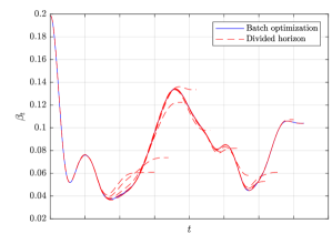
Additional evaluations

Posterior robustness

The computed posterior in Fig. 2 is the population weighted posterior when combining the samples from Sweden’s 21 regions. In Fig. 14 we display the mean posterior $\pm$ 1 standard deviation for each region. The results agree well across this natural bootstrap population albeit with a few outliers.

Figure 14: Posterior mean $\pm$ 1 standard deviation per parameter and across 21 Swedish regions. For the dynamic parameters $R_{t}$ and IFR, the temporal average is displayed.

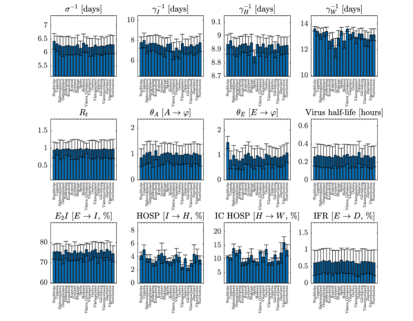
Bootstrap robustness

By the bootstrap procedure presented in Material and Methods, we can investigate the posterior robustness, including estimating the bias due to the approximate likelihood. The inference procedure is repeated on a synthetic data set generated by the mean posterior estimate and with the temporal resolution upscaling procedure for $\beta_{t}$. In Fig. 15 we display 25 such replicates for a few selected regions. Note that these were obtained in a completely off-line fashion and are never corrected against data.

For each region $r=1,\dots,21$ and parameter dimension $k=1,\dots,K$ in the posterior we estimate the bias $\tilde{b}_{r,k}$, as per the description in Material and Methods. The dynamic parameters are here treated as a single parameter, that is, with a single average bias, and together with the static parameters there are $K=12$ in total. We compute three statistics $T=[T_{1},T_{2},T_{3}]$ to characterize the spread: the coefficient of variation (CoV), the coefficient of bias (CoB), and the normalized root-mean-square error (NRMSE),

$$T_{k,r,1}=\text{CoV}=\sigma_{k,r}/\mu_{k,r},\quad T_{k,r,2}=\text{CoB}=|\tilde{b}_{k,r}|/\mu_{k,r},\quad T_{k,r,3}=\text{NRMSE}=\left(\sigma^{2}_{k,r}+\tilde{b}^{2}_{k,r}\right)^{1/2}/\mu_{k,r},$$ (45)

for the standard deviation $\sigma_{k,r}$, the mean $\mu_{k,r}$, and the estimated bias $\tilde{b}_{k,r}$. In Tab. 6, we present the median value per region and statistic $s\in\{1,2,3\}$ over the $K$ parameters,

$$\bar{T}_{r,s}=\text{Median}_{k}\,T_{k,r,s}.$$ (46)

We visualize both the data posterior and the aggregate of all bootstrap replicate posteriors ($n=3$) in Fig. 16. We also compare the daily $R_{t}$ estimate of the actual data posterior and the average from the bootstrap replicates for Uppsala in Fig. 17.

Figure 15: Fully synthetic simulations for a few selected regions with parameters from the national mean posterior, but with upscaled regional $\beta_{t}$. The lines of lighter shades of blue and red are realizations and the solid lines are the mean of the samples. The points are the data points used in the inference.

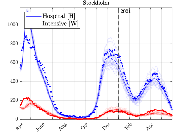
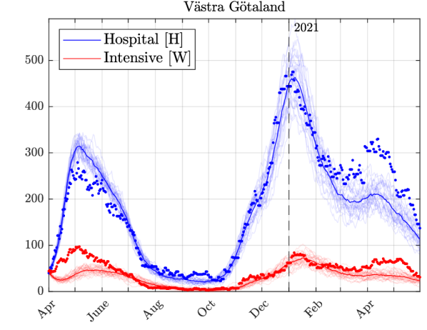
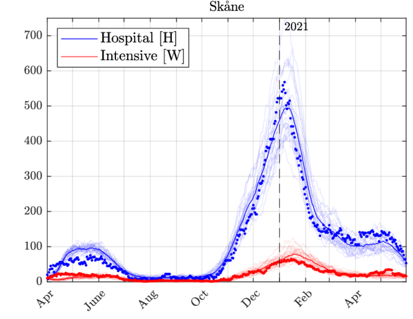
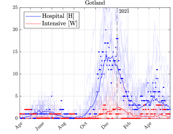
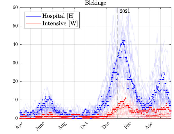
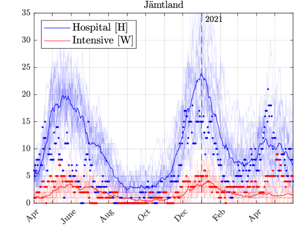
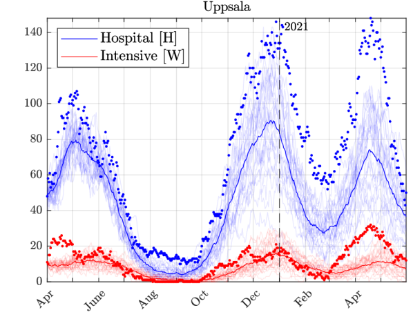
Region	CoV [%]	CoB [%]	NRMSE [%]	$d_{\text{smooth}}[\%]$	Population
Stockholm	6.3	4.9	12	6.6	$2.4\cdot 10^{6}$
Uppsala	13	2.6	15	6.6	$3.8\cdot 10^{5}$
Sodermanland	15	2.0	18	8.1	$3.0\cdot 10^{5}$
Ostergotland	13	4.3	19	7.3	$4.7\cdot 10^{5}$
Jonkoping	14	2.4	18	4.7	$3.6\cdot 10^{5}$
Kronoberg	14	4.0	24	6.9	$2.0\cdot 10^{5}$
Kalmar	16	3.4	23	5.1	$2.5\cdot 10^{5}$
Gotland	29	3.2	32	2.2	$6.0\cdot 10^{4}$
Blekinge	18	3.1	30	13	$1.6\cdot 10^{5}$
Skane	12	3.6	13	5.9	$1.4\cdot 10^{6}$
Halland	16	2.4	24	9.6	$3.3\cdot 10^{5}$
Vastra Gotaland	11	3.9	14	6.2	$1.7\cdot 10^{6}$
Varmland	18	3.5	25	7.7	$2.8\cdot 10^{5}$
Orebro	14	2.6	20	9.4	$3.0\cdot 10^{5}$
Vastmanland	15	5.4	24	4.4	$2.8\cdot 10^{5}$
Dalarna	14	3.6	24	5.7	$2.9\cdot 10^{5}$
Gavleborg	14	2.7	22	4.8	$2.9\cdot 10^{5}$
Vasternorrland	14	2.8	24	4.3	$2.5\cdot 10^{5}$
Jamtland	22	4.1	28	13	$1.3\cdot 10^{5}$
Vasterbotten	20	2.0	23	10	$2.7\cdot 10^{5}$
Norrbotten	18	2.6	26	4.5	$2.5\cdot 10^{5}$

Table 6: Median uncertainty statistic per region: CoV, CoB, and NRMSE as in Eqs. (45)–(46). The smoothing difference $d_{{\text{smooth}}}$ is the mean max relative difference between the pre-processed and raw data $[H,W,D]$ as defined in (6).

Figure 16: Population weighted national average posterior using: actual data (blue) or bootstrapped data (green), for a selected set of parameters. Both posteriors use the same prior (red). The vertical lines indicate the density means: posterior (blue solid), prior (red dashed), and bootstrapped posterior (green dotted). The mean is also annotated in the corresponding color for the posterior estimates.

Figure 17: Reproduction number estimates for the Uppsala region with bootstrap replicas. The Bayesian posterior on the true data yields monthly estimates (blue box-plot) while the quasi-ML estimator is daily (red solid). The aggregate posterior of the bootstrap replicates $[n=3]$ (green box-plot) and the average daily quasi-ML estimator (red dashed) from the bootstrap replicates.

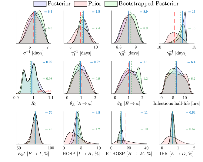
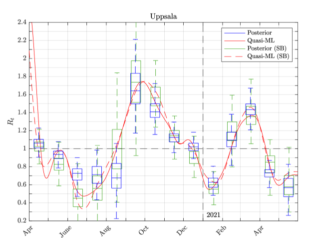
Baseline predictor

To evaluate the predictive performance of our Kalman filter model outside of a model vacuum, we compare to an autoregressive model (AR) model. AR models are common in time-series predictions, and for COVID-19, AR models with auxiliary indicators show significant prediction power [mcdonald2021can]. We consider a single-day forward expanding data window for which we fit the AR model on all data in the window and predict 7 days ahead. This procedure is evaluated across the same data as used in our live reports ($N=25$).

As the Kalman filter, the AR model also uses $[H,W,D]$ as observations. We use Matlab’s arx implementation of the AR model, formally called Vector AR model with Exogenous Variables. The polynomial orders and delays are set from finding good predictions in a mean square error sense on the first 50 days of the dataset. We tune $n_{b}$ and $n_{c}$ by hand, and proposed values for $n_{a}$ by a partial autocorrelation function plot per data dimensions. We find the order of the $A_{q}$ polynomials: $n_{a}=[1,1,1]^{\intercal}$, the $B_{q}$ polynomials: $n_{b}=[0,1,0]^{\intercal}$, and the input-output delay: $n_{c}=[1,1,1]^{\intercal}$ to be close to optimal choices.

In Fig. 18, we visualize the 7-day ahead prediction made by the AR model for Uppsala. In Tab. 7, we present the respective prediction precision by NRMSE and multivariate Energy score [gneiting2008assessing] of the two models along with a repetition of the results from Tab. 1. A closer inspection reveals that the simpler models have a smaller NRMSE and Energy Score than the posterior Kalman filter but with overly pessimistic CrIs. The simple AR model generates good mean-square predictions in a fraction of the training time of our posterior Kalman filter and could likely be improved a bit when it comes to the width of the confidence interval estimate, reducing the Energy score further. The great advantage with our approach lies instead in the fact that the posterior model itself can be disassembled and contains valuable epidemiological information.

Figure 18: Result from the 7-day ahead AR prediction for the Uppsala region with 68% CrI (shaded). The live reporting ($N=25$) for Tabs. 1 and 7 was done in the reporting period indicated towards the second half.

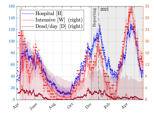
	Hospital (H)	Intensive (W)	Death (D)
Posterior Kalman (68% CrI)	76	72	68
AR	100	100	44
Posterior Kalman (95% CrI)	100	100	96
AR	100	100	92
Posterior Kalman (NRMSE)	25	27	1.9
AR	4.7	12	1.4
Posterior Kalman (Energy score)	84	15	30
AR	18	7.1	24

Table 7: Frequency of all weekly reported predictions (N = 25, Dec 2020–May 2021) for Uppsala that fell inside of the reported CrIs (68/95%, 7 days ahead), the NRMSE, and the multivariate Energy Score evaluated on the following week, thus comparing the performance of the posterior Kalman filter and the AR model.

References

- Abad et al. [2021] Z. S. H. Abad, A. Kline, M. Sultana, M. Noaeen, E. Nurmambetova, F. Lucini, M. Al-Jefri, and J. Lee. Digital public health surveillance: a systematic scoping review. NPJ Digit. Med., 4(1):1–13, 2021. doi: 10.1038/s41746-021-00407-6.
- Alimohamadi et al. [2021] Y. Alimohamadi, H. H. Tola, A. Abbasi-Ghahramanloo, M. Janani, and M. Sepandi. Case fatality rate of COVID-19: a systematic review and meta-analysis. J. Prev. Med. Hyg., 62(2):E311, 2021. doi: 10.15167/2421-4248/jpmh2021.62.2.1627.
- Almgren and Björk [2021] M. Almgren and J. Björk. Kartläggning av skillnader i regionernas insatser för provtagning och smittspårning under coronapandemin. Technical Report ISBN 978-91-525-0257-0, Coronakommissionen S 2020:09, 2021. Underlagsrapport till SOU 2021:89 Sverige under pandemin.
- Altmejd et al. [2023] A. Altmejd, J. Rocklöv, and J. Wallin. Nowcasting COVID-19 statistics reported with delay: A case-study of Sweden and the UK. Int. J. Environ. Res. Publ. Health, 20(4), 2023. doi: 10.3390/ijerph20043040.
- Anderson and May [1981] R. M. Anderson and R. M. May. The population dynamics of microparasites and their invertebrate hosts. Philos. Trans. R. Soc., 291(1054):451–524, 1981. doi: 10.1098/rstb.1981.0005.
- Benson et al. [2021] L. Benson, R. S. Davidson, D. M. Green, A. Hoyle, M. R. Hutchings, and G. Marion. When and why direct transmission models can be used for environmentally persistent pathogens. PLoS Comput. Biol., 17(12):1–26, 12 2021. doi: 10.1371/journal.pcbi.1009652.
- Byrne et al. [2020] A. W. Byrne, D. McEvoy, A. B. Collins, K. Hunt, M. Casey, A. Barber, F. Butler, J. Griffin, E. A. Lane, C. McAloon, et al. Inferred duration of infectious period of SARS-CoV-2: rapid scoping review and analysis of available evidence for asymptomatic and symptomatic COVID-19 cases. BMJ Open, 10(8):e039856, 2020. doi: 10.1136/bmjopen-2020-039856.
- Castro Dopico et al. [2021] X. Castro Dopico, S. Muschiol, M. Christian, L. Hanke, D. Sheward, N. Grinberg, J. Rorbach, G. Bogdanovic, G. Mcinerney, T. Allander, et al. Seropositivity in blood donors and pregnant women during the first year of SARS-CoV-2 transmission in Stockholm, Sweden. J. Intern. Med., 2021. doi: 10.1111/joim.13304.
- COVID-19 Forecasting Team [2022] COVID-19 Forecasting Team. Variation in the COVID-19 infection–fatality ratio by age, time, and geography during the pre-vaccine era: a systematic analysis. The Lancet, 2022. doi: https://doi.org/10.1016/S0140-6736(21)02867-1.
- Davis et al. [2021] J. T. Davis, M. Chinazzi, N. Perra, K. Mu, A. Pastore y Piontti, M. Ajelli, N. E. Dean, C. Gioannini, M. Litvinova, S. Merler, et al. Cryptic transmission of SARS-CoV-2 and the first COVID-19 wave. Nature, 600(7887):127–132, 2021. doi: 10.1038/s41586-021-04130-w.
- Delamater et al. [2019] P. L. Delamater, E. J. Street, T. F. Leslie, Y. T. Yang, and K. H. Jacobsen. Complexity of the basic reproduction number (R0). Emerg. Infect. Dis., 25(1):1, 2019. doi: 10.3201/eid2501.171901.
- Drew et al. [2020] D. A. Drew, L. H. Nguyen, C. J. Steves, C. Menni, M. Freydin, T. Varsavsky, C. H. Sudre, M. J. Cardoso, S. Ourselin, J. Wolf, et al. Rapid implementation of mobile technology for real-time epidemiology of COVID-19. Science, 368(6497):1362–1367, 2020. doi: 10.1126/science.abc0473.
- Edeling et al. [2021] W. Edeling, H. Arabnejad, R. Sinclair, D. Suleimenova, K. Gopalakrishnan, B. Bosak, D. Groen, I. Mahmood, D. Crommelin, and P. V. Coveney. The impact of uncertainty on predictions of the CovidSim epidemiological code. Nat. Comput. Sci., 1(2):128–135, 2021. doi: 10.1038/s43588-021-00028-9.
- Engblom et al. [2020] S. Engblom, R. Eriksson, and S. Widgren. Bayesian epidemiological modeling over high-resolution network data. Epidemics, 32:100399, 2020. doi: 10.1016/j.epidem.2020.100399.
- Fearnhead et al. [2014] P. Fearnhead, V. Giagos, and C. Sherlock. Inference for reaction networks using the linear noise approximation. Biometrics, 70(2):457–466, 2014. doi: 10.1111/biom.12152.
- Folkhälsomyndigheten [2021a] Folkhälsomyndigheten. The infection fatality rate of COVID-19 in Stockholm – technical report. https://www.folkhalsomyndigheten.se/contentassets, 2021a. Online; accessed 2022-01-21.
- Folkhälsomyndigheten [2021b] Folkhälsomyndigheten. Scenarier för fortsatt spridning. https://www.folkhalsomyndigheten.se/smittskydd-beredskap/utbrott/aktuella-utbrott/covid-19/statistik-och-analyser/analys-och-prognoser, 2021b. 2–7. Online; accessed 2022-01-21.
- Folkhälsomyndigheten [2021c] Folkhälsomyndigheten. Påvisning av antikroppar mot SARS-CoV-2 (1) i blodprov från öppenvården, (2) hos blodgivare. https://www.folkhalsomyndigheten.se/contentassets, 2021c. Online; accessed 2022-01-21.
- Folkhälsomyndigheten [2021d] Folkhälsomyndigheten. Veckorapport om covid-19, vecka 39. https://www.folkhalsomyndigheten.se/globalassets/statistik-uppfoljning/smittsamma-sjukdomar/veckorapporter-covid-19/2021/covid-19-veckorapport-2021-vecka-39-final.pdf, 2021d. Online; accessed 2022-02-09.
- Gabry et al. [2019] J. Gabry, D. Simpson, A. Vehtari, M. Betancourt, and A. Gelman. Visualization in Bayesian workflow. J. R. Stat. Soc. Ser. A, 182(2):389–402, 2019. doi: 10.1111/rssa.12378.
- Galani et al. [2022] A. Galani, R. Aalizadeh, M. Kostakis, A. Markou, N. Alygizakis, T. Lytras, P. G. Adamopoulos, J. Peccia, D. C. Thompson, A. Kontou, et al. SARS-CoV-2 wastewater surveillance data can predict hospitalizations and ICU admissions. Sci. Total Environ., 804:150151, 2022. doi: 10.1016/j.scitotenv.2021.150151.
- Garcia-Ptacek et al. [2021] S. Garcia-Ptacek, H. Xu, M. Annetorp, V. B. Jerlardtz, T. Cederholm, M. Engström, M. Kivipelto, L. G. Lundberg, C. Metzner, M. Olsson, J. S. Nyvang, C. S. Öberg, E. Åkesson, D. Religa, and M. Eriksdotter. Temporal trends in hospitalizations and 30-day mortality in older patients during the COVID pandemic from March 2020 to July 2021. medRxiv preprint medRxiv:2021.12.22.21268237, 2021. doi: 10.1101/2021.12.22.21268237.
- Gatto et al. [2020] M. Gatto, E. Bertuzzo, L. Mari, S. Miccoli, L. Carraro, R. Casagrandi, and A. Rinaldo. Spread and dynamics of the COVID-19 epidemic in Italy: Effects of emergency containment measures. Proc. Natl. Acad. Sci. USA, 117(19):10484–10491, 2020. doi: 10.1073/pnas.2004978117.
- Gelman et al. [1995] A. Gelman, J. B. Carlin, H. S. Stern, and D. B. Rubin. Bayesian data analysis. Chapman and Hall/CRC, 1995. doi: 10.1201/b16018.
- Guidotti and Ardia [2020] E. Guidotti and D. Ardia. COVID-19 data hub. J. Open Source Softw., 5(51):2376, 2020. doi: 10.21105/joss.02376.
- Haario et al. [2001] H. Haario, E. Saksman, and J. Tamminen. An adaptive Metropolis algorithm. Bernoulli, 7(2):223–242, 2001. doi: 10.2307/3318737.
- Haug et al. [2020] N. Haug, L. Geyrhofer, A. Londei, E. Dervic, A. Desvars-Larrive, V. Loreto, B. Pinior, S. Thurner, and P. Klimek. Ranking the effectiveness of worldwide COVID-19 government interventions. Nat. Hum. Behav., 4(12):1303–1312, 2020. doi: 10.1038/s41562-020-01009-0.
- Hawryluk et al. [2021] I. Hawryluk, H. Hoeltgebaum, S. Mishra, X. Miscouridou, R. P. Schnekenberg, C. Whittaker, M. Vollmer, S. Flaxman, S. Bhatt, and T. A. Mellan. Gaussian process nowcasting: Application to COVID-19 mortality reporting. In Uncertainty Artif. Intell., pages 1258–1268, 2021.
- Ilin et al. [2021] C. Ilin, S. Annan-Phan, X. H. Tai, S. Mehra, S. Hsiang, and J. E. Blumenstock. Public mobility data enables COVID-19 forecasting and management at local and global scales. Sci. Rep., 11(1):1–11, 2021. doi: 10.1038/s41598-021-92892-8.
- Imran et al. [2022] M. Imran, U. Qazi, and F. Ofli. TBCOV: Two Billion Multilingual COVID-19 Tweets with Sentiment, Entity, Geo, and Gender Labels. Data, 7(1):8, 2022. doi: 10.3390/data7010008.
- Irons and Raftery [2021] N. J. Irons and A. E. Raftery. Estimating SARS-CoV-2 infections from deaths, confirmed cases, tests, and random surveys. Proc. Natl. Acad. Sci. USA, 118(31), 2021. doi: 10.1073/pnas.2103272118.
- Jordan et al. [2021] E. Jordan, D. E. Shin, S. Leekha, and S. Azarm. Optimization in the context of COVID-19 prediction and control: A literature review. IEEE Access, 2021. doi: 10.1109/ACCESS.2021.3113812.
- Karolinska universitetslaboratoriet [2022] Karolinska universitetslaboratoriet. Luftvägspatogener prov analyserade av Karolinska Universitetslaboratoriet till och med vecka 5 2022. https://www.karolinska.se/globalassets/global/2-funktioner/funktion-kul/klinisk-mikrobiologi/epidemiologi/rapport-influensa--och-rs-virus-och-andra-luftvagspatogener.pdf, 2022. Online; accessed 2022-02-09.
- Keeling et al. [2021] M. J. Keeling, E. M. Hill, E. E. Gorsich, B. Penman, G. Guyver-Fletcher, A. Holmes, T. Leng, H. McKimm, M. Tamborrino, L. Dyson, and M. J. Tildesley. Predictions of COVID-19 dynamics in the UK: Short-term forecasting and analysis of potential exit strategies. PLoS Comput. Biol., 17(1):1–20, 2021. doi: 10.1371/journal.pcbi.1008619.
- Kelly and Cowling [2013] H. Kelly and B. J. Cowling. Case fatality: rate, ratio, or risk? Epidemiology, 24(4):622–623, 2013. doi: 10.1097/EDE.0b013e318296c2b6.
- Kennedy et al. [2022] B. Kennedy, H. Fitipaldi, U. Hammar, M. Maziarz, N. Tsereteli, N. Oskolkov, G. Varotsis, C. A. Franks, D. Nguyen, L. Spiliopoulos, H.-O. Adami, J. Björk, S. Engblom, K. Fall, A. Grimby-Ekman, J.-E. Litton, M. Martinell, A. Oudin, T. Sjöström, T. Timpka, C. H. Sudre, M. S. Graham, J. L. du Cadet, A. T. Chan, R. Davies, S. Ganesh, A. May, S. Ourselin, J. C. Pujol, S. Selvachandran, J. Wolf, T. D. Spector, C. J. Steves, M. F. Gomez, P. W. Franks, and T. Fall. App-based COVID-19 syndromic surveillance and prediction of hospital admissions in COVID Symptom Study Sweden. Nat. Commun., 13:2110, 2022. doi: 10.1038/s41467-022-29608-7.
- Lavezzo et al. [2020] E. Lavezzo, E. Franchin, C. Ciavarella, G. Cuomo-Dannenburg, L. Barzon, C. Del Vecchio, L. Rossi, R. Manganelli, A. Loregian, N. Navarin, et al. Suppression of a SARS-CoV-2 outbreak in the Italian municipality of Vo’. Nature, 584(7821):425–429, 2020. doi: 10.1038/s41586-020-2488-1.
- Li et al. [2020] Q. Li, X. Guan, P. Wu, X. Wang, L. Zhou, Y. Tong, R. Ren, K. S. Leung, E. H. Lau, J. Y. Wong, et al. Early transmission dynamics in Wuhan, China, of novel coronavirus–infected pneumonia. N. Engl. J. Med., 2020. doi: 10.1056/NEJMoa2001316.
- Liu and Rocklöv [2021] Y. Liu and J. Rocklöv. The reproductive number of the delta variant of SARS-CoV-2 is far higher compared to the ancestral SARS-CoV-2 virus. J. Travel Med., 2021. doi: 10.1093/jtm/taab124.
- Menni et al. [2020] C. Menni, A. M. Valdes, M. B. Freidin, C. H. Sudre, L. H. Nguyen, D. A. Drew, S. Ganesh, T. Varsavsky, M. J. Cardoso, J. S. E.-S. Moustafa, et al. Real-time tracking of self-reported symptoms to predict potential COVID-19. Nat. Med., 26(7):1037–1040, 2020. doi: 10.1038/s41591-020-0916-2.
- Reinhart et al. [2021] A. Reinhart, L. Brooks, M. Jahja, A. Rumack, J. Tang, S. Agrawal, W. Al Saeed, T. Arnold, A. Basu, J. Bien, et al. An open repository of real-time COVID-19 indicators. Proc. Natl. Acad. Sci. USA, 118(51), 2021. doi: 10.1073/pnas.2111452118.
- Rippinger et al. [2021] C. Rippinger, M. Bicher, C. Urach, D. Brunmeir, N. Weibrecht, G. Zauner, G. Sroczynski, B. Jahn, N. Mühlberger, U. Siebert, et al. Evaluation of undetected cases during the COVID-19 epidemic in Austria. BMC Infec. Dis., 21(1):1–11, 2021. doi: 10.1186/s12879-020-05737-6.
- Rossman et al. [2020] H. Rossman, A. Keshet, S. Shilo, A. Gavrieli, T. Bauman, O. Cohen, E. Shelly, R. Balicer, B. Geiger, Y. Dor, et al. A framework for identifying regional outbreak and spread of COVID-19 from one-minute population-wide surveys. Nat. Med., 26(5):634–638, 2020. doi: 10.1038/s41591-020-0857-9.
- Russo et al. [2020] L. Russo, C. Anastassopoulou, A. Tsakris, G. N. Bifulco, E. F. Campana, G. Toraldo, and C. Siettos. Tracing day-zero and forecasting the COVID-19 outbreak in Lombardy, Italy: A compartmental modelling and numerical optimization approach. PLoS ONE, 15(10):e0240649, Oct. 2020. ISSN 19326203. doi: 10.1371/journal.pone.0240649. e0240649.
- Saguti et al. [2021] F. Saguti, E. Magnil, L. Enache, M. P. Churqui, A. Johansson, D. Lumley, F. Davidsson, L. Dotevall, A. Mattsson, E. Trybala, et al. Surveillance of wastewater revealed peaks of SARS-CoV-2 preceding those of hospitalized patients with COVID-19. Water Res., 189:116620, 2021. doi: 10.1016/j.watres.2020.116620.
- Salje et al. [2020] H. Salje, C. T. Kiem, N. Lefrancq, N. Courtejoie, P. Bosetti, J. Paireau, A. Andronico, N. Hozé, J. Richet, C.-L. Dubost, et al. Estimating the burden of SARS-CoV-2 in France. Science, 369(6500):208–211, 2020. doi: 10.1126/science.abc3517.
- Shinde et al. [2020] G. R. Shinde, A. B. Kalamkar, P. N. Mahalle, N. Dey, J. Chaki, and A. E. Hassanien. Forecasting models for coronavirus disease (COVID-19): a survey of the state-of-the-art. SN Comput. Sci., 1(4):1–15, 2020. doi: 10.1007/s42979-020-00209-9.
- Socialstyrelsen [2020] Socialstyrelsen. Avlidna och covid-19. https://www.socialstyrelsen.se/statistik-och-data/statistik/statistik-om-covid-19/statistik-over-antal-avlidna-i-covid-19, 2020. Online; accessed 2022-02-09.
- Soltesz et al. [2020] K. Soltesz, F. Gustafsson, T. Timpka, J. Jaldén, C. Jidling, A. Heimerson, T. B. Schön, A. Spreco, J. Ekberg, Ö. Dahlström, et al. The effect of interventions on COVID-19. Nature, 588(7839):E26–E28, 2020. doi: 10.1038/s41586-020-3025-y.
- Sveriges Kommuner och Regioner [2021] Sveriges Kommuner och Regioner. Meddelande från styrelsen - Överenskommelse mellan Staten och Sveriges Kommuner och Regioner om ökad nationell testning och smittspårning för covid-19, 2021. https://skr.se/download/18.32563d7d1784aa279ece298a/1618741812524/WEBB-17-OK-Staten-SKR-Covid-19.pdf, 2021. Online; accessed 2022-04-01.
- van den Driessche [2017] P. van den Driessche. Reproduction numbers of infectious disease models. Infect. Disease Model., 2(3):288–303, 2017. doi: 10.1016/j.idm.2017.06.002.
- Widgren et al. [2018] S. Widgren, S. Engblom, U. Emanuelson, and A. Lindberg. Spatio-temporal modelling of verotoxigenic Escherichia coli O157 in cattle in Sweden: exploring options for control. Vet. Res., 49(1):1–13, 2018. doi: 10.1186/s13567-018-0574-2.
- Winblad et al. [2022] U. Winblad, A.-K. Swenning, and D. Spangler. Soft law and individual responsibility: a review of the Swedish policy response to COVID-19. Health Econ. Policy Law, 17(1):48–61, 2022. doi: 10.1017/S1744133121000256.
- Wood [2010] S. N. Wood. Statistical inference for noisy nonlinear ecological dynamic systems. Nature, 466(7310):1102–1104, 2010. doi: 10.1038/nature09319.
- Wu et al. [2020] J. T. Wu, K. Leung, and G. M. Leung. Nowcasting and forecasting the potential domestic and international spread of the 2019-nCoV outbreak originating in Wuhan, China: a modelling study. The Lancet, 395(10225):689–697, 2020. doi: 10.1016/S0140-6736(20)30260-9.
- Wu et al. [2021] J. T. Wu, K. Leung, T. T. Lam, M. Y. Ni, C. K. Wong, J. Peiris, and G. M. Leung. Nowcasting epidemics of novel pathogens: lessons from COVID-19. Nat. Med., 27(3):388–395, 2021. doi: 10.1038/s41591-021-01278-w.
- Wynants et al. [2020] L. Wynants, B. Van Calster, G. S. Collins, R. D. Riley, G. Heinze, E. Schuit, M. M. Bonten, D. L. Dahly, J. A. Damen, T. P. Debray, et al. Prediction models for diagnosis and prognosis of covid-19: systematic review and critical appraisal. BMJ, 369, 2020. doi: 10.1136/bmj.m1328.
- Alene et al. [2021] M. Alene, L. Yismaw, M. A. Assemie, D. B. Ketema, B. Mengist, B. Kassie, and T. Y. Birhan. Magnitude of asymptomatic COVID-19 cases throughout the course of infection: A systematic review and meta-analysis. PLoS ONE, 16(3):e0249090, 2021. doi: 10.1371/journal.pone.0249090.
- Alimohamadi et al. [2020] Y. Alimohamadi, M. Taghdir, and M. Sepandi. Estimate of the basic reproduction number for COVID-19: a systematic review and meta-analysis. J. Prev. Med. Public Health, 53(3):151, 2020. doi: 10.3961/jpmph.20.076.
- Brazeau et al. [2020] N. Brazeau, R. Verity, S. Jenks, H. Fu, C. Whittaker, P. Winskill, I. Dorigatti, P. Walker, S. Riley, R. P. Schnekenberg, et al. Report 34: COVID-19 infection fatality ratio: estimates from seroprevalence. https://www.imperial.ac.uk/mrc-global-infectious-disease-analysis/covid-19/report-34-ifr, 2020.
- [7] C19, Swedish COVID-19 data aggregator. c19.se. https://c19.se/compare, 2020. Online; accessed 2022-04-01.
- Dhouib et al. [2021] W. Dhouib, J. Maatoug, I. Ayouni, N. Zammit, R. Ghammem, S. B. Fredj, and H. Ghannem. The incubation period during the pandemic of COVID-19: a systematic review and meta-analysis. Syst. Rev., 10(101):1–14, 2021. doi: 10.1186/s13643-021-01648-y.
- Diekmann et al. [2010] O. Diekmann, J. A. P. Heesterbeek, and M. G. Roberts. The construction of next-generation matrices for compartmental epidemic models. J. Roy. Soc. Interface, 7(47):873–885, 2010. doi: 10.1098/rsif.2009.0386.
- Engblom and Widgren [2017] S. Engblom and S. Widgren. Data-driven computational disease spread modeling: from measurement to parametrization and control. In Disease Modeling and Public Health: Part A, volume 36 of Handbook of statistics, chapter 11, pages 305–328. Elsevier, 2017. doi: 10.1016/bs.host.2017.05.005.
- Ferretti et al. [2020] L. Ferretti, C. Wymant, M. Kendall, L. Zhao, A. Nurtay, L. Abeler-Dörner, M. Parker, D. Bonsall, and C. Fraser. Quantifying SARS-CoV-2 transmission suggests epidemic control with digital contact tracing. Science, 368(6491):eabb6936, 2020. doi: 10.1126/science.abb6936.
- Folkhälsomyndigheten [2020] Folkhälsomyndigheten. Bekräftade fall av covid-19 i sverige. https://www.arcgis.com/sharing/rest/content/items/b5e7488e117749c19881cce45db13f7e/data, 2020. Online; accessed 2022-04-01.
- Folkhälsomyndigheten [2021b] Folkhälsomyndigheten. Påvisning av antikroppar mot SARS-CoV-2 (1) i blodprov från öppenvården, (2) hos blodgivare. https://www.folkhalsomyndigheten.se/contentassets, 2021b. Online; accessed 2022-01-21.
- Folkhälsomyndigheten [2021c] Folkhälsomyndigheten. Aktuellt reproduktionstal (R-tal). https://www.folkhalsomyndigheten.se/smittskydd-beredskap/utbrott/aktuella-utbrott/covid-19/statistik-och-analyser/analys-och-prognoser, 2021c. Online; accessed 2022-01-13.
- Gneiting et al. [2008] T. Gneiting, L. I. Stanberry, E. P. Grimit, L. Held, and N. A. Johnson. Assessing probabilistic forecasts of multivariate quantities, with an application to ensemble predictions of surface winds. TEST, 17(2):211–235, 2008. doi: 10.1007/s11749-008-0114-x.
- Marin et al. [2012] J.-M. Marin, P. Pudlo, C. P. Robert, and R. J. Ryder. Approximate Bayesian computational methods. Stat. Comp., 22(6):1167–1180, 2012. doi: 10.1007/s11222-011-9288-2.
- McDonald et al. [2021] D. J. McDonald, J. Bien, A. Green, A. J. Hu, N. DeFries, S. Hyun, N. L. Oliveira, J. Sharpnack, J. Tang, R. Tibshirani, et al. Can auxiliary indicators improve COVID-19 forecasting and hotspot prediction? Proc. Natl. Acad. Sci. USA., 118(51), 2021. doi: 10.1073/pnas.2111453118.
- Sisson et al. [2018] S. A. Sisson, Y. Fan, and M. Beaumont. Handbook of approximate Bayesian computation. CRC Press, 2018.
- Socialstyrelsen [2020a] Socialstyrelsen. Avlidna och covid-19. https://www.socialstyrelsen.se/statistik-och-data/statistik/statistik-om-covid-19/statistik-over-antal-avlidna-i-covid-19, 2020a. Online; accessed 2022-02-09.
- Socialstyrelsen [2020b] Socialstyrelsen. Vård och covid-19. https://www.socialstyrelsen.se/statistik-och-data/statistik/statistik-om-covid-19/statistik-om-slutenvard-av-patienter-med-covid-19, 2020b. Online; accessed 2022-02-09.
- Statistikmyndigheten SCB [2019] Statistikmyndigheten SCB. Antal pendlare per län och kommun, 2018. https://www.scb.se/hitta-statistik/statistik-efter-amne/arbetsmarknad/sysselsattning-forvarvsarbete-och-arbetstider/registerbaserad-arbetsmarknadsstatistik-rams/pong/tabell-och-diagram/antal-pendlare-per-lan-och-kommun-2018, 2019. Online; accessed 2020-03-22.
- Statistikmyndigheten SCB [2020] Statistikmyndigheten SCB. Sveriges befolkningspyramid. https://www.scb.se/hitta-statistik/sverige-i-siffror/manniskorna-i-sverige/sveriges-befolkningspyramid, 2020. Online; accessed 2020-04-08.
- Strålin et al. [2021] K. Strålin, E. Wahlström, S. Walther, A. M. Bennet-Bark, M. Heurgren, T. Lindén, J. Holm, and H. Hanberger. Mortality trends among hospitalised COVID-19 patients in sweden: a nationwide observational cohort study. The Lancet Reg. Health-Europe, 4:100054, 2021. doi: 10.1016/j.lanepe.2021.100054.
- Svenska Intensivvårdsregistret [2020] Svenska Intensivvårdsregistret. Mortalitet 30 dagar, Coronafall. https://portal.icuregswe.org/siri/en/report/corona.mort?filter=d5d1d908-cd6a-8db0-e5ec-8c76b834d20, 2020. Online; accessed 2022-02-09.
- Van Doremalen et al. [2020] N. Van Doremalen, T. Bushmaker, D. H. Morris, M. G. Holbrook, A. Gamble, B. N. Williamson, A. Tamin, J. L. Harcourt, N. J. Thornburg, S. I. Gerber, et al. Aerosol and surface stability of SARS-CoV-2 as compared with SARS-CoV-1. N. Engl. J. Med., 382(16):1564–1567, 2020. doi: 10.1056/NEJMc2004973.