Highest Cusped Waves for the Burgers-Hilbert equation
Joel Dahne
Javier Gómez-Serrano
Abstract
In this paper we prove the existence of a periodic highest, cusped,
traveling wave solution for the Burgers-Hilbert equation
and give its asymptotic behaviour at
. The proof combines careful asymptotic analysis and a
computer-assisted approach.
1 Introduction
The Burgers-Hilbert equation [25] is a
nonlinear wave model, in the periodic setting given by
(1)
Here is the Hilbert transform which, for
, is defined by
The equation was first used by Marsden and Weinstein in 1983 as a
second order approximation for the evolution of the boundary of a
simply connected vortex patch in two dimensions [44].
More recently Biello and Hunter used it to serve as an approximation
for small slope vorticity fronts [4]. The
validity of this approximation was recently proved
[28].
For small initial data in , estimates for the
lifespan were proved by Hunter and Ifrim
[26], see also [27].
Global existence of weak solutions for initial data in
was established by Bressan and Nguyen, in which
case the solution lies in
for
[5]. Bressan and Zhang constructed locally in time
piecewise smooth solutions with a single, logarithmic, shock
[6]. Stability and uniqueness of these solutions in a
larger class of solutions were shown by Krupa and Vasseur
[42].
Numerical simulations have shown formation of shocks in finite time
[4, 25]. Castro,
Córdoba and Gancedo proved finite time blow up of the
-norm with for initial data
satisfying that there exists a point with
and
[8]. Saut and Wang proved shock formation in finite time
[50]. Solutions that develop an asymptotic self-similar
shock at a single point with an explicitly computable blowup profile
were constructed by Yang [55].
The Burgers-Hilbert equation occurs as a special case in the family of
fractional KdV equations given by
(2)
Here
and the parameter may in general take any real value. For
and we get the classical KdV and
Benjamin-Ono equations. For it reduces to the
Burgers-Hilbert equation.
For the fractional KdV equation exhibits finite
time blow [8, 29]. That this blowup happens in terms
of wave breaking was proved for by Hur and
Tao [31, 30] and for by Oh and
Pasqualotto [47]. See [41] for a
numerical study and also [11]. For other
results see e.g. [19] for existence time,
[49] for well-posedness and [39, 40] for some results for related equations.
In this work we are concerned with traveling wave solutions of the
Burgers-Hilbert equation (1). The study of traveling waves
is an important topic in fluid dynamics, see e.g. [23]
for a recent overview of traveling water waves. The traveling wave
assumption , where denotes the
wave speed, gives us
(3)
The Burgers-Hilbert equation has an analytic branch of even,
zero-mean, -periodic, smooth traveling wave solutions
bifurcating from constant solutions [25]. If
we let be the bifurcation parameter and
, be the solution with its
corresponding wave speed, then as we have
Castro, Córdoba and Zheng [10] proved that this
branch exists in the range with
and fails to exist for
. Moreover they proved an enhanced lifespan
estimate for perturbations of compared to the
results in [26]. In
[25], Hunter remarks that this branch
presumably ends in a highest wave which is not smooth at its crest, as
is common for equations of this type. In this paper we prove the
existence of a highest cusped wave and give its behaviour at the
crest. More precisely we prove the following theorem:
Theorem 1.1.
There is a -periodic traveling wave of
(3), which behaves asymptotically at as
Remark 1.2.
We don’t expect the remainder term
in Theorem 1.1 to be
sharp. The estimate follows from the choice of our space.
The notion of highest traveling waves exist for a large number of
equations. For the free boundary Euler equation Stokes argued that if
there exists a singular solution with a steady profile it must have an
interior angle of at the crest
[51]. This is known as the Stokes conjecture
and was proved in 1982 [1]. For the Whitham equation
[54] the existence of a highest cusped traveling wave
was conjectured by Whitham in [53]. Its existence,
together with its regularity, was recently proved by
Ehrnström and Wahlén [18]. They conjectured that the
wave is convex between its crests and also its precise asymptotic
behaviour. This conjecture was proved by Enciso, Gómez-Serrano and
Vergara [20]. See also [17]
for some recent remarks. For the fractional KdV equations the
traveling waves assumption allows us to write the equation as
(4)
There has recently been much progress related to highest waves to this
family of equations. For Bruell and Dhara proved the
existence of highest traveling waves which are Lipschitz at their cusp
[7]. Very recently Ørke proved their existence for
for the (inhomogeneous) fractional KdV equations
as well as the fractional Degasperis-Procesi equations, together with
their optimal -Hölder regularity
[48]. Hildrum and Xue prove a similar result
for another class of equations, including the (homogeneous) fractional
KdV equations for
[24].
The results in [18, 7, 48, 24] are all based
on global bifurcation arguments, bifurcating from the constant
solution and proving that the branch must end in a highest wave which
is not smooth at its crest. The proof of the convexity of the highest
cusped wave for the Whitham equation in [20]
uses a completely different approach. The problem is first rephrased
as a fixed point problem, the existence and properties of the fixed
point is then related to inequalities for certain constants that
appear in the reduction. These inequalities are then checked using a a
computer assisted proof. In this paper we use a similar approach for
proving Theorem 1.1.
The ansatz allows us to rewrite
(3) as an equation that does not explicitly depend on
the wave speed . Proving the existence of a solution can be
rewritten as a fixed point problem by considering the ansatz
where is an explicit, carefully chosen, approximate
solution and is an explicit weight factor. Proving the
existence of a fixed point can be reduced to checking an inequality
involving three constants, , and ,
that only depend on the choice of and , see Proposition
2.2. This inequality is checked by bounding
, and using a computer assisted
proof, see Lemmas 7.1, 7.2
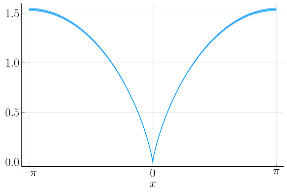
and 7.3. These bounds are highly non-trivial, in
particular is given by the supremum of a function on
the interval which attains its maximum around
. A plot of the function is given in Figure
1.
Figure 1: An enclosure of the function on the interval
. The thin line is the approximation
and the width of the thick line is computed using the bound of
.
One of the key difficulties is the construction of the approximate
solution . Due to the singularity at it is not
possible to use a trigonometric polynomial alone, it would converge
very slowly and have the wrong asymptotic behaviour. Pure products of
powers and logarithms, , have the issue that
they are not periodic and do not interact well with the operator
. Instead we take inspiration from the construction in
[20] and consider a combination of trigonometric
polynomials and Clausen functions of different orders, defined as
for and by analytic continuation otherwise. We also make use
of their derivatives with respect to the order, for which we use the
notation
These functions are -periodic, non-analytic at and
behave well with respect to . In particular
, which
corresponds to the behaviour we expect in Theorem 1.1.
However, directly applying the ideas from [20]
for the construction does not work since it is not easy to determine
the next term in the expansion. Instead we go through the fractional
KdV equations for , for this family of equations
the same ideas do work and we then study the limit .
Remark 1.3.
From the representation of and the bounds for , given
in Section 8, it is possible to compute
quantitative bounds for properties of the solution.
It is possible to enclose the first Fourier coefficient of the
solution , and hence also . For the first
Fourier coefficient is given by , taking into
account the bounds for we can compute the enclosure
for the first Fourier coefficient of .
This agrees with the results from Castro, Córdoba and Zheng
[10] that the branch of solutions break down
for somewhere between and
. It also agrees with their (unpublished) numerical
results indicating that the branch ends around
[9].
It is also possible to enclose the mean of , which gives the
wavespeed for a corresponding zero-mean . From the
expression of (see (11)) it is straightforward to
compute the mean of . Taking into account
the bounds for we get the enclosure for the
mean of .
An important part of our work is the interplay between traditional
mathematical tools and rigorous computer calculations. Traditional
numerical methods typically only compute approximate results, to be
able to use the results in a proof we need the results to be
rigorously verified. The basis for rigorous calculations is interval
arithmetic, pioneered by Moore in the 1970’s [46]. Due to
improvements in both computational power as well as well as great
improvements in software it has become possible to use computer
assisted tools in many more problems. The main idea with interval
arithmetic is to do arithmetic not directly on real numbers but on
intervals with computer representable endpoints. Given a function
, an interval extension of is an
extension to intervals satisfying that for an interval x,
is an interval satisfying
for all . In particular this allows us to prove
inequalities for the function , for example the right endpoint of
gives an upper bound of on the interval
x. For an introduction to interval arithmetic and rigorous
numerics we refer the reader to the books [46, 52]
and to the survey [21] for a specific treatment of
computer assisted proofs in PDE. For all the calculations in this
paper we make use of the Arb library [36] for ball
(intervals represented as a midpoint and radius) arithmetic. It has
good support for many of the special functions we use
[38, 32, 37],
Taylor arithmetic (see e.g. [34]) as well as
rigorous integration [33].
The paper is organized as follows. In Section
2 we reduce the proof of Theorem
1.1 to a fixed point problem. In Section
3 we give a brief overview of properties of
the Clausen functions that are relevant for the construction of
, in Section 4 we give the construction
of . Section 5 is devoted to the
approach for bounding and , Section
6 to studying the linear operator that appears in
the construction of the fixed point problem. The computer assisted
proofs giving bounds for , and are
given in Section 7. Finally we give the
proof of Theorem 1.1 in Section
8.
Three appendices are given at the end of the paper. Appendix
A gives some technical details for how
to compute enclosures of functions around removable singularities.
Appendix B is concerned with computing
enclosures of the Clausen functions and Appendix
C with the rigorous numerical integration
needed for bounding .
2 Reduction to a fixed point problem
In this section we reduce the problem of proving Theorem
1.1 to proving the existence of a fixed point for a certain
operator. We start with the following lemma which motivates the notion
of highest wave (see also [24, Theorem
3.4])
Lemma 2.1.
Let be a nonconstant, even solution of
(3) which is nondecreasing on , then
on .
Proof.
We start by proving that under these assumptions
. Since is even we can write the
Hilbert transform of as
Integration by parts gives us
For and we have
For this follows from that is increasing as
a distance to a multiple of and that is
closer to zero than is to zero or , the
case can be reduced to the previous case by switching
and and using that is odd. It follows that
Since we get .
Furthermore is nonconstant and continuous so we have
in some open set, giving us .
As a consequence, any continuous, nonconstant, even function which is
nondecreasing on that satisfy (3) almost
everywhere must satisfy . The maximal possible
height is thus given by and due to the function being even and
nondecreasing on the maximal height has to be attained
at .
Now, the ansatz inserted in
(3) gives an equation which does not explicitly depend
on the wave speed . Indeed, inserting this gives us
(5)
Note that a solution of this equation gives a solution of
(3) for any wave speed . This is to be expected
due to the Galilean change of variables
which leaves (3) invariant. In particular, taking
equal to the mean of gives a zero mean solution. For a highest
wave we expect to have , giving us .
Integrating (5) gives us
(6)
Here is the operator
(7)
It is the integral of the Hilbert transform with the constant of
integration taken such that , this ensures
that any solution of (6) satisfies . Note that
any solution of (6) is a solution of
(5) and hence gives a solution to
(3).
To reduce the problem to a fixed point problem we write as one,
explicit, approximate solution of (6) and one unknown
term. More precisely we make the ansatz
(8)
where is an explicit, carefully chosen, approximate
solution of (6) and
. By taking
, proving Theorem
1.1 reduces to proving existence of
such that the given ansatz is a
solution of (6).
By collecting all the linear terms in we can write this as
Now let denote the operator
(9)
Denote the weighted defect of the approximate solution by
and let
Then we can write the above as
Assuming that is invertible we can rewrite this as
(10)
Hence proving the existence of such that that is
a solution to (6) reduces to proving the existence of a
fixed point of the operator .
Next we reduce the problem of proving that has a fixed point to
checking an inequality for three numbers that depend only on the
choice of and . We let denote the
norm of a linear
operator .
Proposition 2.2.
Let ,
and
. If and
they satisfy the inequality
then for
and
we have
1.
;
2.
with for all
.
Proof.
Using that and are even it can be checked that
Since the operator is invertible and an
upper bound of the norm of the inverse is given by
, moreover takes even functions to even
functions and hence so will . This gives us
The choice of then gives
Next we have and hence
Where since
.
∎
3 Clausen functions
We here give definitions and properties of the Clausen functions that
are used in Sections 4,
5 and 6. For more details
about the Clausen functions see Appendix B.
The Clausen functions are related to the polylogarithm through
They behave nicely with respect to the Hilbert transform, for which we
have
In many cases we want to work with functions which are normalised to
be zero at , for which we use the notation
With this notation we get for the operator ,
From [20] we have the following expansion for
and , valid for ,
For the functions and we will
mainly make use of and , for
which we have the following expansions [2, Eq. 16],
valid for ,
Where is the Stieltjes constant and
. Bounds for the tails are given in Lemmas
B.3 and B.4.
4 Construction of the approximate solution
In this section we give the construction of the approximate solution
. As a first step we determine the coefficient for the
leading term in the asymptotic expansion.
Lemma 4.1.
Let be a solution of (6) with the asymptotic
behaviour
close to zero, with . Then the coefficient is given
by .
Proof.
For the asymptotic behaviour of the left hand side in
(6) we directly get
To get the asymptotic behaviour of in the right
hand side we go through the Clausen function
, which has the asymptotic behaviour
Since we
have
giving us
For and to have the same
asymptotic behaviour we must therefore have
which gives us the result.
∎
In addition to having the correct asymptotic behaviour we want
to be a good approximate solution of (6), in the
sense that we want the defect,
to be small for . The hardest part is to make
small locally near the singularity at , this is done
by studying the asymptotic behaviour of
. Ones the defect
is sufficiently small near it can be made small globally by
adding a suitable trigonometric polynomial.
The construction is similar to that in [20], the
main difference is that the asymptotic behaviour is more complicated
in our case. We take to be a combination of three parts:
1.
The first part is the term
, where the coefficient is
chosen to give the right asymptotic behaviour according to Lemma
4.1.
2.
The second part is chosen to make the defect small near
and, similarly to in [20], it is
given by a sum of Clausen functions.
3.
The third part is chosen to make the defect small globally and
is given by a trigonometric polynomial.
More precisely the approximation is given by
(11)
To ensure that the leading asymptotics are determined by
we require that .
We want to chose the values of and to make the
defect small near . Taking
gives us that the
leading term in the expansion of
is of order
. A natural choice would then be to take the next
term as a multiple of , for which
behaves like .
However, its contribution to the term of
and turns out to
exactly cancel out and we are left with no improvement to the
asymptotic behaviour.
Instead we take inspiration from the fractional KdV equations
(4), which for reduces to the
Burgers-Hilbert equation. To chose and we study
the limit . For the
fractional KdV equations, like the Burgers-Hilbert equation, admits a
highest cusped traveling wave solution, as recently proved in
[48]. In a forthcoming
[12] work we show that the traveling waves
asymptotically at behave like
, with
Following the same approach as in Section 2
proving the existence of a highest cusped wave for the fractional KdV
equations can be reduced to studying the equation
where
. By
studying the asymptotic behaviour of
and following the same
reasoning as in [20] a suitable approximation
for this equation is given by
with
and a solution of
One can numerically solve for by considering the
asymptotic expansion of the defect. As we have
and . Numerically one
also sees that , in such a way that
remains bounded. The other
coefficients, for , all remain bounded.
Furthermore we note that as approaches , the function
approaches
. The remaining part,
is numerically seen to converge to a function as , as
long as is increased as we approach . This
gives a hint on how to choose and for ,
we take it according to
For this we fix some close to and compute
as well as the coefficients . We then
take ,
for and
As long as is sufficiently close to and is
sufficiently high this gives a small enough defect close to .
While not obvious from the expression of we do have
, as required.
The coefficients are then taken to make the defect small
globally. This is done by taking equally spaced points
on the interval and
numerically solving the non-linear system
In the computations we use (giving
), and
.
Remark 4.2.
The approximation only needs to be an approximate solution
to the equation, as opposed to the coefficient for
, which has to match exactly to obtain the
right asymptotic behaviour.
With this approximation we get
(12)
Furthermore we have the following asymptotic expansions for the
approximation, which we give without proof since they follow directly
from the expansions of the Clausen and trigonometric functions.
Lemma 4.3.
The approximation given by equation (11) has the
asymptotic expansions
and
valid for , where
5 Bounding and
Recall that
where
For fixed which is not too small we can compute accurate
enclosures of as well as using interval arithmetic.
This allows us to compute
for some fixed . As the numerators and
denominators tend to zero in both and and we need to
handle the removable singularities. We start with the following lemma:
Lemma 5.1.
The function is positive and
bounded at and for it has the expansion
Proof.
The expansion follows directly from the expansion of given
in Lemma 4.3 and canceling the
factor.
The function goes to zero at and is
bounded nearby and by construction and are taken
such that for . This
means that all terms except tend to zero as
. The value at will hence be given by
.
∎
In light of this lemma we do the split
The second factor can then be bounded using the lemma. For the first
factor it is enough to notice that it tends to zero at and
is increasing in on . For we do the split
The first factor can be handled by noticing that it tends to zero at
and is increasing in , the second factor is handled
using the above lemma. What remains is to handle the third factor,
which is done in the following lemma:
Lemma 5.2.
The function
is non-zero and bounded at and for it has the
expansion
Division by gives the required expansion. Note that
the two leading terms in and
exactly cancel out, this is needed for the
result to be bounded near .
∎
6 Analysis of and bounding
In this section we give more details about the operator defined
by
The integrand of has a singularity at . It is
therefore natural to split the integral into two parts
where
The following two lemmas give information about the sign of
and , allowing us to remove the absolute
value.
Lemma 6.1.
For all the function is
decreasing and continuous in for and has the
limits
Moreover, the unique root, , is decreasing in and
satisfies the inequality
Proof.
The left and right limits are easily checked and it is clear that
the function is continuous in on the interval. To show that it
is decreasing in we split the into three terms and
differentiate, giving us
We want to prove that this is negative. Note that
and that is positive on the
interval , hence it is enough to check
which follows immediately from the monotonicity of on the
interval . This proves the existence of a unique root
on the interval .
To prove that is decreasing in it is enough to prove
that is decreasing in . Differentiating with
respect to gives us
which we want to prove is negative. Letting
and using that for
it is enough to show that
This holds since is concave, as
following from and
.
Finally, to see that it
is enough to check that for the root is given by
and that
together with the monotonicity in .
∎
Lemma 6.2.
For we have for all
.
Proof.
The function is strictly convex on the
domain . This follows from the fact that
is strictly convex and decreasing and is strictly
concave on the interval. It immediately follows that
∎
With these two lemmas we can slightly simplify and
, we get
and
Similarly to in the previous section we divide the interval
, on which we take the supremum, into two parts,
and .
For the interval we split as
See Appendix C for details on how
, and are computed.
For the interval write as
The factor is handled by Lemma
5.1 as before. For the two remaining terms
we have the following two lemmas:
Lemma 6.3.
For with we have
where
Proof.
As a first step we split into one main term and
one remainder term. We can write as
Using that
where , and similarly for the other
log-sin terms, we can split as
where
Note that for small , is close to one, and the
corresponding log-terms will therefore be small. We split
as
Focusing in we note that for we have
(16)
Hence
We have
and
if we let
this gives us
For we will give a uniform bound of
in on the interval and use this to simplify the
integrand. Note that ,
and all lie on the interval . The
function is analytic around and the
first two terms in the Taylor expansion are zero, by Taylor’s
Theorem we hence have
To easier bound we note that the function in
(17) is increasing in for . To
see this focus on the part
which we want to show is decreasing in . If we let
we can
write the above as
Differentiating we have
since is concave on this is non-positive. To
see that indeed is concave on this interval it is enough to
check that
is negative on , which follows from that the
coefficients in the Taylor expansion at all are negative.
This means that the supremum for is attained at
and it reduces to
∎
To use these lemmas in the computer assisted proof the first step is
to compute enclosures of , , ,
and . For this can be done directly using Taylor
arithmetic. For and we have removable
singularities that need to be dealt with, this can be done using the
approach described in Appendix A. For
and we refer to Appendix
C.
For Lemma 6.3 it is straightforward to compute
enclosures of all the terms in the upper bound by using monotonicity
properties in . For Lemma 6.4 the
expression for the upper bound is more complicated. In particular
several of the terms contain removable singularities at ,
these are handled using the approach described in Appendix
A. As an example we show how to bound
the other terms can be done in a similar way.
Lemma 6.5.
The function
is bounded from above by and is decreasing in on the
interval .
Proof.
Taking the limit gives the value , it
is hence enough to prove that it is decreasing in .
Differentiating with respect to gives us
The sign is given by that of
For we get the upper bound
which is negative.
∎
7 Bounds for , and
We are now ready to give bounds for , and
. Recall that they are given by
In each case we split the interval into two parts,
and , with varying
for the different cases, and threat them separately. For the interval
we use the asymptotic bounds for the different
functions that were introduced in the previous two sections. For the
interval we evaluate the functions directly using
interval arithmetic. For the direct evaluation the only complicated
part is the computation of in , where we
proceed as discussed in Section 6 and
Appendix C.
Consider the problem of enclosing the maximum of on some
interval to some predetermined tolerance. The main idea is to
iteratively bisect the interval into smaller and smaller
subintervals. At every iteration we compute an enclosure of on
each subinterval. From these enclosures a lower bound of the maximum
can be computed. We then discard all subintervals for which the
enclosure is less than the lower bound of the maximum, the maximum
cannot be attained there. For the remaining subintervals we check if
their enclosure satisfies the required tolerance, in that case we
don’t bisect them further. If there are any subintervals left we
bisect them and continue with the next iteration. In the end, either
when there are no subintervals left to bisect or we have reached some
maximum number of iterations (to guarantee that the procedure
terminates), we return the maximum of all subintervals that were not
discarded. This is guaranteed to give an enclosure of the maximum of
on the interval.
If we are able to compute Taylor series of the function we can
improve the performance of this procedure significantly (see e.g.
[14, 13] where a similar approach is
used). Consider a subinterval , instead of computing an
enclosure of we compute a Taylor polynomial at the
midpoint and an enclosure of the remainder term such that
for . We then have
(18)
To compute we isolate the roots of
on and evaluate on the roots as well as the endpoints
of the interval. In practice the computation of involves
computing an enclosure of the Taylor series of on the full
interval . Since this includes the derivative we can as an
extra optimization check if the derivative is non-zero, in which case
is monotone and it is enough to evaluate on either the
left or the right endpoint of , depending on the sign of the
derivative.
The above procedures can easily be adapted to instead compute the
minimum of on the interval, joining them together we can thus
compute the extrema on the interval. In some cases we don’t care about
computing an enclosure of the maximum, but only to prove that it is
bounded by some value. Instead of using a tolerance we then discard
any subintervals for which the enclosure of the maximum is less than
the bound.
In most cases we bisect the subintervals at the midpoint, meaning that
the interval would be bisected into the two
intervals and
. However, when the magnitude of
and are very different it can be beneficial to
bisect at the geometric midpoint (see e.g. [22]), in
that case we split the interval into
and
, where we assume that
.
We split the computation of the bounds for ,
and into three lemmas. The proof of the lemmas are computer
assisted and we give some details about the process. The lemmas are
stated as upper bounds, but in the process of proving them we do
compute actual enclosures of the values.
The code 111Available at
https://github.com/Joel-Dahne/BurgersHilbertWave.jl, the
results in the paper are from commit
d7863475d1c4e9d8f49da716b4ef2dc936c3dab9. for the computer assisted
part is implemented in Julia [3]. The main tool for the
rigorous numerics is Arb [35] which we use through
the Julia wrapper Arblib.jl
222https://github.com/kalmarek/Arblib.jl. Many of the
basic interval arithmetic algorithms, such as isolating roots or
enclosing maximum values, are implemented in a separate package,
ArbExtras.jl
333https://github.com/Joel-Dahne/ArbExtras.jl. For
finding the coefficients and of
we make use of non-linear solvers from NLsolve.jl
[45].
The computations were done on an AMD Ryzen 9 5900X processor with 32
GB of RAM using 20 threads and when timings are given it refers to
this configuration. In most cases the computations are multithreaded
and make use of all available threads. The computations were done
using 100 bits of precision.
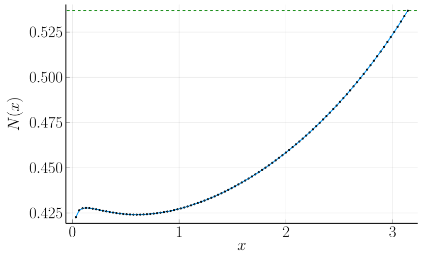
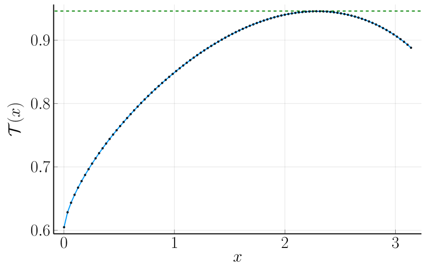
Lemma 7.1.
The constant satisfies the inequality
.
Proof.
A plot of on the interval is given in Figure
2(a) and hints at the maximum being attained at
. A good guess for the maximum value is thus given by
.
We take . For the interval we
don’t compute an enclosure of the maximum but only prove that it is
bounded by .
For the interval we compute an enclosure of the
maximum. This gives us
which is upper bounded by .
We are able to compute Taylor expansions of in both the
asymptotic and non-asymptotic case as long as the subinterval
doesn’t contain zero. This allows us to use the better version of
the algorithm, based on the Taylor polynomial, for enclosing the
maximum and fall back to the naive version, where no information
about the derivatives is used, for the subintervals containing zero.
We use a Taylor expansion of degree , which is enough to pick
up the monotonicity after only a few bisections in most cases. The
runtime is about 5 seconds, most of it for handling the interval
.
∎
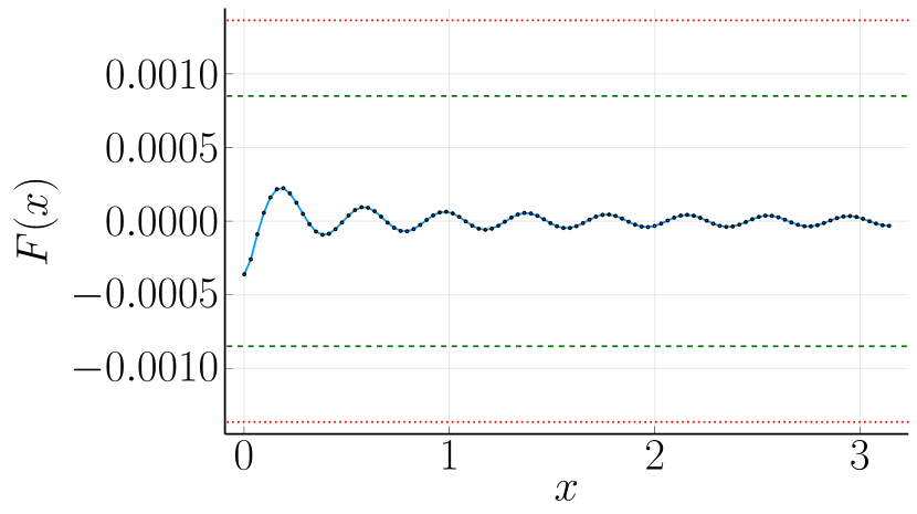
Lemma 7.2.
The constant satisfies the inequality
.
Proof.
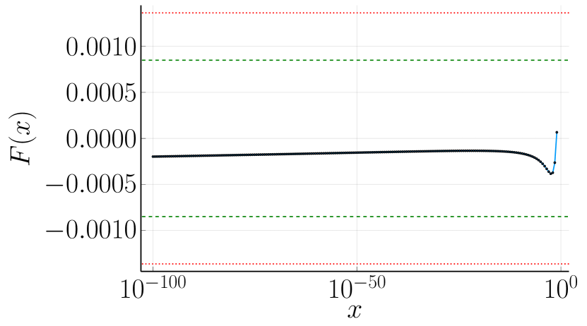
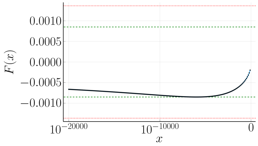
A plot of on the interval is given in Figure
3(a), however this plot doesn’t reveal the full picture of
what happens close to . Figures 3(b)
and 3(c) show a log-plot of on the
intervals and
respectively. In the latter of these figures we can see that
has an extrema between and , this
turns out to be where the maximum of is attained. Note that
these numbers are extremely small, too small to be represented even
in standard quadruple precision (binary128), though Arb has
no problem handling them.
We take . Handling the interval
is straightforward and we get the enclosure
. The interval
is more delicate due to the extrema being attained
for such an extremely small .
In general evaluation with the asymptotic version of is much
faster than the non-asymptotic version. However, for the interval
we have to do a huge number of subdivisions and it
is therefore beneficial to optimize it slightly more. The terms in
the expansions used for computing are given in Lemmas
5.1 and 5.2, they
contain factors of the form and
with varying coefficients and
exponents . When gets smaller more and more of these
terms become negligible. To reduce the number of terms in the
expansions we can collapse all negligible terms into one remainder
term. If we fix some then on the interval
with we have for
and
with a similar expression for . In this way we can take all
terms with an exponent greater than and put them into one
single term with the exponent . If is small enough so
that is negligible this will still give a good
enclosure.
For this we split the interval into four parts,
, ,
and ,
with ,
and .
For the first two intervals we take , on the
third we take it to be and on the fourth we keep all
terms. For the expansion from Lemma 5.1
this leaves us with , and terms respectively.
For the expansion from Lemma 5.2 we get
, and terms.
The interval is taken such that a single
evaluation of gives a good enough enclosure, we have
. The
bulk of the work is for the second interval, it needs to be split
into more than subintervals and the final enclosure for
the maximum is . The third
interval, , is split into more than
subintervals, with the enclosure
. For
it suffices to split it in around
subintervals and we get the enclosure
.
We are able to compute Taylor expansions of in both the
asymptotic and non-asymptotic case as long as the subinterval
doesn’t contain zero, this allows us to use the better version of
the algorithm for enclosing the maximum and fall back to the naive
version for the subintervals containing zero. We use a Taylor
expansion of degree in all cases. On the intervals
,
and we bisect at the geometric midpoint
instead of bisecting at the arithmetic midpoint. The runtime is
about 15 minutes.
∎
Lemma 7.3.
The constant satisfies the inequality
.
Proof.
A plot of on the interval is given
in Figure 2(b). It hints at the maximum being attained
around .
We take and start by computing the maximum on
, this gives us the enclosure
.
For the interval we make use of the asymptotic
expansions from Lemmas 6.3 and
6.4. Since these only give upper bounds we are
not able to compute an enclosure of on this
interval. However, since the maximum is attained on the interval
we only need prove that is
bounded by this value on . Hence the maximum for
the full interval is given by that on and we get
which is upper bounded by .
In this case we do not have access to Taylor series of
in either the asymptotic or non-asymptotic case.
This means we have to rely on the naive version for bounding the
maximum. On the interval there is one
optimization that we can do. involves a division
by and for this function we have access to Taylor
series, we therefore compute a tighter enclosure of this using a
bound.
The total runtime for the computation is around 90 seconds, the
majority for handling the interval .
∎
(a)
(b)
Figure 2: Plot of the functions and on the
interval . The dashed green lines show the upper
bounds and as given in Lemmas
7.1 and 7.3
(a)
(b)
(c)
Figure 3: Plot of the function on the intervals ,
and . The
dashed green line shows the upper bound as
given in Lemma 7.2. The dotted red line
shows , which is the
value we want the defect to be smaller than.
is a traveling wave solution to (1). This proves the
existence of a -periodic highest cusped traveling wave.
To get the asymptotic behaviour we note that
Hence
and
as we wanted to show.
∎
Appendix A Removable singularities
In several cases we have to compute enclosures of functions with
removable singularities. For example the function
comes up when computing through equation
(23) and has a removable singularity
whenever is a positive even integer. In this appendix we explain
how to compute rigorous enclosures at and around these points. For
this we need a way to handle the removable singularity. Let
We have the following lemma for handling functions with removable
singularities:
Lemma A.1.
Let and let be an interval
containing zero. Consider a function with a zero of order
at and such that is absolutely
continuous on . Then for all we have
for some between and . Furthermore, if
is absolutely continuous for
we have
for some between and .
Proof.
The first statement follows directly from expanding in a
Taylor series with a remainder term on Lagrange form and dividing by
, using that for .
For the second statement we start by noting that
(19)
The Taylor expansion of with the remainder term
in integral form is
From [15, Sec. 15.4.24] we get that this is zero for
. The second sum in (22) we can
rewrite as
For the terms are zero since .
For we use [15, Sec. 15.2.4] to write the
inner sum as
From [15, Sec. 15.4.24] we get that this is zero for
and for it is given by
. This gives us that
(22) can be written as
which is what we wanted to show.
We are now interested in the remainder term of
(21) when inserted into
(19), we get
We first show that the sum is non-negative. Using
[15, Sec. 15.2.4] we have
By [43, Theorem 3.2] (see also [16, Theorem
2]), have no
roots on the interval and for it is positive,
it is hence positive on . Since the sum is positive the
integral can be written as
for some between and . Simplifying further we get
which is exactly the expression given for the remainder term.
∎
Using this lemma we can compute enclosures at and around removable
singularities as long as we have good control over and its
derivatives.
Example A.2.
Consider the function with a
removable singularity at . If we let we can
write the function as
If we let and take ,
then for the second factor the lemma then tells us that
for some between and . Using interval arithmetic
we can easily compute enclosure of the coefficients for the
polynomial as well as . For the second factor we
can’t directly apply the lemma, instead we rewrite it in terms of
the reciprocal gamma function, . If we let
we have
The function has a root at and we can thus apply
the lemma on . An enclosure of the coefficients
for the polynomial as well as the remainder term can be computed
using the implementation of the reciprocal gamma function in Arb.
Appendix B Computing enclosures of Clausen functions
To be able to compute bounds of ,
and it is critical that we can compute accurate
enclosures of and , including expansions in
the argument and derivatives in the parameter. We here go through how
these enclosures are computed. We make use of several different
special functions, most of them with implementations in Arb (see e.g.
[38, 32]). In several cases we
encounter removable singularities, they are all dealt with as
explained in Appendix A, see in
particular example A.2.
We start by going through how to compute and
for . Since both and
are -periodic we can reduce it to or
.
For and we get directly from the defining sum that
and . For both
functions typically diverge at .
For we can compute the Clausen functions by going
through the polylog function,
However it is computationally beneficial (about 40% faster in
general) to instead go through the periodic zeta function
[15, Sec. 25.13],
for which we have
For the periodic zeta function can be written as
[15, Eq. 25.13.2]
Taking the real and imaginary part we get, for ,
(23)
(24)
This formulation works well as long as is not a non-negative
integer. For non-negative integers we have to handle some removable
singularities.
For the functions
and
diverge and needs to
be handled differently. The Laurent series of the zeta function gives
us
(25)
where is the Stieltjes constant. The sum is referred to
as the deflated zeta function, it has an implementation in Arb and we
denote it by . Writing the Clausen
functions in terms of the deflated zeta function gives us
The expression for is now well defined, all terms are
finite, for around zero. For we also have to handle
the removable singularity of .
For equal to a positive integer, has a pole.
For with even we get a removable singularity in
and for with odd
we get that has a
removable singularity. For the other parity of we instead have
to look at the zeta function. For integer we have
where is the Bernoulli polynomial
[15, Eq. 25.6.3]. Since
[15, Eq. 24.4.3] we have
for odd and
for even . This means that
has a removable singularity for odd and
has a removable singularity for even . This allows us to handle
all removable singularities in (23) and
(24) when is a positive integer.
B.1 Interval arguments
We are now ready to compute enclosures for interval arguments. Let
and
be two finite intervals, we are interested in computing an enclosure
of and . Due
to the periodicity we can reduce it to three different cases for
x
1.
x doesn’t contain a multiple of , by adding
or subtracting a suitable multiple of we can assume that
;
2.
x has a diameter of at least , it then
covers a full period and can without loss of generality be taken as
;
3.
x contains a multiple of but has a diameter
less than , by adding or subtracting a suitable multiple of
we can take x such that
.
We begin by considering the case when .
It is possible to evaluate (23) and
(24) directly, treating as an
interval, however this gives huge overestimations as soon as
x is not a very tight interval. For we make use
of the following lemma, see also [20, Lemma B.1].
Lemma B.1.
For all the Clausen function is
monotone in on the interval . For it is
non-increasing.
For we use equation (24)
together with [15, Eq. 25.11.25] to get
which sign depends only on the value . In particular, for
we have
so is
decreasing for .
∎
Since is even around it follows that if
then the extrema of
are attained at either ,
or, if , . This allows
us to compute very tight enclosures of in
the argument x. The function is in general
not monotone. We handle it by computing and enclosure of the
derivative
, if the
enclosure of the derivative doesn’t contain zero then the function is
monotone and we evaluate it at the endpoints, if the derivative
contains zero we instead use the midpoint approximation
where is the midpoint
of x.
For we assume that since
the value is typically unbounded otherwise (in which case we return an
indeterminate result). We get an enclosure of
by evaluating at the critical points
and . For we use the
trivial bound
to get the enclosure
.
For the final case, when ,
we also assume that . We handle
by using the eveness and monotonicity in
. If then the extrema are
attained at and ,
otherwise the extrema are attained at and . For
we check if it is increasing on
x by checking if and
, where we have used that
is decreasing for . If it is increasing we
evaluate at the endpoints, otherwise we have the trivial bound
In all the above cases we could reduce the problem of enclosing the
Clausen functions on x to evaluating them on, a subset of,
, (or if ),
, (the midpoint) and . In all
cases except we have so we can use
(23) and
(24).
For s we get two different cases depending on if
s contains a non-negative integer or not.
When s doesn’t contain a non-negative integer the
formulations (23) and
(24) are well defined. However, similarly
as for x, direct evaluation gives large overestimations
when s is not very tight. In this case there is no
monotonicity to use, instead we compute a tighter enclosure using a
Taylor expansion as in (18). One exception to this
is the modified Clausen function , for which we have
the following result
Lemma B.2.
For and the function
is decreasing in .
Proof.
We have
Since for all terms in
the sum have the same sign. That it is decreasing in then
follows easily from the monotonicity of .
∎
This means that for we only have to evaluate on
and to get an enclosure. In practice
is only every used with so this is enough
go get good bounds.
When s contains a non-negative integer we have to handle
the removable singularities in (23) and
(24) as described in the beginning of the
section. The required derivatives can generally be computed directly
with Arb, this is the case for the reciprocal gamma function,
, as well as . There is an
implementation of the deflated zeta function
in Arb, however it only supports
exactly equal to , and not intervals containing , and can
therefore not be used directly. In our application this case does
however not occur, so it is not an issue.
B.2 Expansion in
We now go through how to compute expansions of the Clausen functions
in the argument .
Around any point the functions are analytic and it is
straightforward to compute the Taylor expansions by differentiating
directly, using that and
.
At we then have the following asymptotic expansions
[20]
(26)
(27)
These expressions work well as long as is not a positive
integer. For positive integers we have to handle the poles of
at non-positive integers and the pole of at
.
For with positive even integers the only
problematic term is
which has a removable singularity. Similarly for with
positive odd integers . For with positive odd
integers and with positive even integers the
singularities are not removable, however in this paper we don’t
encounter this case.
With the above we are able to compute expansions at to
arbitrarily high degree. What remains is to bound the tails of the
sums in (26) and
(27). For this we have the following
lemma, see also [20, Lemma 2.1]. We omit the
proof since it is very similar to that in [20].
Lemma B.3.
Let , and , we then have
the following bounds for the tails in equations
(26) and
(27)
B.3 Derivatives in
For and we use
(23) and
(24) and differentiate directly in .
When is not an integer this is handled directly using Taylor
arithmetic, for integers we use the approach in Appendix
A to handle the removable
singularities.
To get asymptotic expansions in we take the expansions
(26) and (27)
and differentiate them with respect to . Giving us
(28)
(29)
These formulas work well when is not a positive odd integer for
or a positive even integer for
and the derivatives can be computed using
Taylor series. We mostly make use of the functions
and , in which case the expansions can be computed
explicitly using [2, Eq. 16], for we have
Where is the Stieltjes constant and
. To bound the tails we have the following
lemma:
Lemma B.4.
Let , and , we then
have the following bounds:
Here is given recursively by
where is the polygamma function. It is given by a sum
of terms of the form
If we have the following bounds
with . If
we have
with .
Proof.
We give the proof for the first case, the other one is similar. We
have the functional identity
If we let
we have
This gives us
We are thus interested in bounding
for .
For we start by noting that
Hence
and, in particular,
For we start from
. Differentiating this
we get
where is given recursively by
This gives us
For we have
Since we have and hence
which is decreasing in . Giving us
Combining the bounds for , and
we have
Using that this simplifies to
This proves the first part of the statement.
Using that we can
compute for any fixed . It is clear that all terms of
will be on the form
From the integral representation [15, Eq. 5.9.15] it
follows that for we have , using
that we get . For
and it follows from the integral
representation
that is decreasing in . For we
then have the bound
This gives us
Focusing on the sum we rewrite it as
Here it can be noted that the sum is given by the Lerch transcendent
. Hence
Consider a constant such that
(30)
with this we can bound the Lerch transcendent as
If we take
then
the first inequality in (30) is satisfied. For the
second inequality to be satisfied we must then have
, if this does not hold we can
sum the first few terms of the series explicitly to work with a
larger . Note that this method for bounding sum is the same as
that used by Arb in the, currently unreleased,
implementation444https://fredrikj.net/blog/2022/02/computing-the-lerch-transcendent/
of the Lerch transcendent.
Putting all of this together we arrived at the bound
∎
Appendix C Rigorous integration with singularities
We here explain how to compute enclosures of the integrals
, and in the non-asymptotic
case, as well as how to enclose and occurring in
Lemmas 6.3 and 6.4. Recall
that
The integrand for has a (integrable) singularity at
and the integrand for has one at . As a
first step we split these off to handle them separately. Let
For and we have the following lemma
Lemma C.1.
We have
for some in the image of
for . Furthermore
for some in the image of for
.
Proof.
We give the proof for , the other one is similar.
The factor in the integrand of
is bounded in on the interval
and the integrand has a constant sign, hence
there exists in the range of
on this interval such that
(31)
It is therefore enough to compute an enclosure of this integral. For
this we use that to write it as
Using that we get
Integrating from to gives us
which proves the result.
∎
What remains is computing , and .
In this case the integrands are bounded everywhere on the intervals of
integration and we enclose the integrals using the rigorous numerical
integrator implemented by Arb [33]. For
functions that are analytic on the interval the integrator uses
Gaussian quadratures with error bounds computed through complex
magnitudes, we therefore need to evaluate the integrands on complex
intervals. When the function is not analytic it falls back to naive
enclosures using interval arithmetic. The only non-trivial part is
bounding the integrand for near , where it is
bounded but not analytic. For this we start by splitting it as
For the first two terms the only problematic part is the factor
, we note that it is zero at
and differentiating it gives us
If
then the derivative is positive and we can thus get an enclosure by
checking that this inequality holds and using monotonicity. This
leaves us with the third term,
which is also zero at and for the monotonicity we have the
following lemma
Lemma C.2.
For and the function
is decreasing in .
Proof.
Differentiating we have
Since the denominator is positive it is enough to show that
Since the factor
is positive, multiplication by
makes it negative. Using that
an upper bound is
hence given by
If we let this becomes
Using that for and
we get the upper bound
Splitting gives
Using that and
it reduces to
which is a quadratic expression in , which can easily be
checked to be negative on .
∎
For enclosing and recall that
Both integrands are bounded, by splitting as
they are also analytic except at and for
and for . For the integrand is easily
seen to be increasing for and it can be bounded near
using that. The integrand for is not monotone, to
bound it we split it into three terms
with
It is then enough to bound , and .
Differentiating we have
For we get the unique root on the interval
, we can thus use monotonicity of as long as we
avoid this point. For and we are looking for the
zeros of
respectively. For both and
are increasing, hence is
increasing. From the limits
and it follows that
has exactly one root on . This root can easily be
isolated using interval arithmetic and we can then use monotonicity of
as long as we avoid this root. The function is
also monotone, to see this we differentiate, giving us
The sign is determined by
A lower bound is given by
that this is positive follows from the inequality .
This proves that is monotone, we can then use the same
approach as for to isolate the unique critical point.
Acknowledgments
JD and JGS were partially supported by the ERC Starting Grant
ERC-StG-CAPA-852741. JGS was partially supported by NSF through Grant
NSF DMS-1763356. This material is based upon work supported by the
National Science Foundation under Grant No. DMS-1929284 while JD and
JGS were in residence at the Institute for Computational and
Experimental Research in Mathematics in Providence, RI, during the
program “Hamiltonian Methods in Dispersive and Wave Evolution
Equations”. JD was partially supported by the Swedish-American
foundation for the visit. We are also thankful for the hospitality of
the Princeton Department of Mathematics, the Uppsala University
Department of Mathematics and the Brown University Department of
Mathematics where parts of this paper were done. This work is
supported by the Spanish State Research Agency, through the Severo
Ochoa and María de Maeztu Program for Centers and Units of Excellence
in R&D (CEX2020-001084-M).
References
[1]C.. Amick, L.. Fraenkel and J.. Toland
“On the Stokes conjecture for the wave of extreme form”
In Acta Mathematica148Institut Mittag-Leffler, 1982, pp. 193–214
DOI: 10.1007/bf02392728
[2]D.. Bailey and J.. Borwein
“Computation and structure of character polylogarithms with applications to character Mordell–Tornheim–Witten sums”
In Math. Comp.85.297American Mathematical Society (AMS), 2015, pp. 295–324
DOI: 10.1090/mcom/2974
[3]Jeff Bezanson, Alan Edelman, Stefan Karpinski and Viral B. Shah
“Julia: A Fresh Approach to Numerical Computing”
In SIAM Rev.59.1Society for Industrial & Applied Mathematics (SIAM), 2017, pp. 65–98
DOI: 10.1137/141000671
[4]Joseph Biello and John K. Hunter
“Nonlinear Hamiltonian waves with constant frequency and surface waves on vorticity discontinuities”
In Comm. Pure Appl. Math.63.3Wiley, 2009, pp. 303–336
DOI: 10.1002/cpa.20304
[5]Alberto Bressan and Khai T. Nguyen
“Global Existence of Weak Solutions for the Burgers–Hilbert Equation”
In SIAM Journal on Mathematical Analysis46.4Society for Industrial & Applied Mathematics (SIAM), 2014, pp. 2884–2904
DOI: 10.1137/140957536
[6]Alberto Bressan and Tianyou Zhang
“Piecewise smooth solutions to the Burgers–Hilbert equation”
In Communications in Mathematical Sciences15.1International Press of Boston, 2017, pp. 165–184
DOI: 10.4310/cms.2017.v15.n1.a7
[7]Gabriele Bruell and Raj Narayan Dhara
“Waves of maximal height for a class of nonlocal equations with homogeneous symbols”, 2018
arXiv:1810.00248v1 [math.AP]
[8]Angel Castro, Diego Córdoba and Francisco Gancedo
“Singularity formations for a surface wave model”
In Nonlinearity23.11IOP Publishing, 2010, pp. 2835–2847
DOI: 10.1088/0951-7715/23/11/006
[9]Ángel Castro, Diego Córdoba and Fan Zheng, Personal communication
[10]Ángel Castro, Diego Córdoba and Fan Zheng
“Stability of traveling waves for the Burgers-Hilbert equation”, 2021
arXiv:2103.02897 [math.AP]
[11]Kyle R. Chickering, Ryan C. Moreno-Vasquez and Gavin Pandya
“Asymptotically self-similar shock formation for 1d fractal Burgers equation”, 2021
arXiv:2105.15128v2 [math.AP]
[12]Joel Dahne
“Highest cusped waves for a family of fractional KdV equations” In preparation, 2022
[13]Joel Dahne, Javier Gómez-Serrano and Kimberly Hou
“A counterexample to Payne’s nodal line conjecture with few holes”
In Commun. Nonlinear Sci.103Elsevier BV, 2021, pp. 105957
DOI: 10.1016/j.cnsns.2021.105957
[14]Joel Dahne and Bruno Salvy
“Computation of Tight Enclosures for Laplacian Eigenvalues”
In SIAM J. Sci. Comput.42.5Society for Industrial & Applied Mathematics (SIAM), 2020, pp. A3210–A3232
DOI: 10.1137/20m1326520
[15]“NIST Digital Library of Mathematical Functions” F. W. J. Olver, A. B. Olde Daalhuis, D. W. Lozier, B. I. Schneider, R. F. Boisvert, C. W. Clark, B. R. Miller, B. V. Saunders, H. S. Cohl, and M. A. McClain, eds., http://dlmf.nist.gov/, Release 1.1.4 of 2022-01-15
URL: http://dlmf.nist.gov/
[16]D. Dominici, S.J. Johnston and K. Jordaan
“Real zeros of hypergeometric polynomials”
In Journal of Computational and Applied Mathematics247Elsevier BV, 2013, pp. 152–161
DOI: 10.1016/j.cam.2012.12.024
[17]Mats Ehrnström, Katerina Nik and Christoph Walker
“A direct construction of a full family of Whitham solitary waves”, 2022
arXiv:2204.03274v1 [math.AP]
[18]Mats Ehrnström and Erik Wahlén
“On Whitham’s conjecture of a highest cusped wave for a nonlocal dispersive equation”
In Annales de l’Institut Henri Poincaré C, Analyse non linéaire36.6Elsevier BV, 2019, pp. 1603–1637
DOI: 10.1016/j.anihpc.2019.02.006
[19]Mats Ehrnström and Yuexun Wang
“Enhanced Existence Time of Solutions to the Fractional Korteweg–de Vries Equation”
In SIAM J. Math. Anal.51.4Society for Industrial & Applied Mathematics (SIAM), 2019, pp. 3298–3323
DOI: 10.1137/19m1237867
[20]Alberto Enciso, Javier Gómez-Serrano and Bruno Vergara
“Convexity of Whitham’s highest cusped wave”, 2018
arXiv:1810.10935 [math.AP]
[21]Javier Gómez-Serrano
“Computer-assisted proofs in PDE: a survey”
In SeMA Journal76.3Springer ScienceBusiness Media LLC, 2019, pp. 459–484
DOI: 10.1007/s40324-019-00186-x
[22]Javier Gómez-Serrano and Rafael Granero-Belinchón
“On turning waves for the inhomogeneous Muskat problem: A computer-assisted proof”
In Nonlinearity27.6IOP Publishing, 2014, pp. 1471–1498
DOI: 10.1088/0951-7715/27/6/1471
[23]Susanna Haziot, Vera Hur, Walter Strauss, J. Toland, Erik Wahlén, Samuel Walsh and Miles Wheeler
“Traveling water waves — the ebb and flow of two centuries”
In Quarterly of Applied Mathematics80.2American Mathematical Society (AMS), 2022, pp. 317–401
DOI: 10.1090/qam/1614
[24]Fredrik Hildrum and Jun Xue
“Periodic Hölder waves in nonsmooth fractional KdV equations”, 2022
arXiv:2202.07363v1 [math.AP]
[25]John K. Hunter
“The Burgers–Hilbert Equation”
In Theory, Numerics and Applications of Hyperbolic Problems IICham: Springer International Publishing, 2018, pp. 41–57
DOI: 10.1007/978-3-319-91548-7˙3
[26]John K. Hunter and Mihaela Ifrim
“Enhanced Life Span of Smooth Solutions of a Burgers–Hilbert Equation”
In SIAM J. Math. Anal.44.3Society for Industrial & Applied Mathematics (SIAM), 2012, pp. 2039–2052
DOI: 10.1137/110849791
[27]John K. Hunter, Mihaela Ifrim, Daniel Tataru and Tak Kwong Wong
“Long time solutions for a Burgers-Hilbert equation via a modified energy method”
In Proc. Amer. Math. Soc.143.8American Mathematical Society (AMS), 2015, pp. 3407–3412
DOI: 10.1090/proc/12215
[28]John K. Hunter, Ryan C. Moreno-Vasquez, Jingyang Shu and Qingtian Zhang
“On the approximation of vorticity fronts by the Burgers–Hilbert equation”
In Asymptotic AnalysisIOS Press, 2021, pp. 1–37
DOI: 10.3233/asy-211724
[29]Vera Mikyoung Hur
“On the formation of singularities for surface water waves”
In Communications on Pure and Applied Analysis11.4American Institute of Mathematical Sciences (AIMS), 2012, pp. 1465–1474
DOI: 10.3934/cpaa.2012.11.1465
[30]Vera Mikyoung Hur
“Wave breaking in the Whitham equation”
In Advances in Mathematics317Elsevier BV, 2017, pp. 410–437
DOI: 10.1016/j.aim.2017.07.006
[31]Vera Mikyoung Hur and Lizheng Tao
“Wave breaking for the Whitham equation with fractional dispersion”
In Nonlinearity27.12IOP Publishing, 2014, pp. 2937–2949
DOI: 10.1088/0951-7715/27/12/2937
[32]F. Johansson
“Fast and rigorous computation of special functions to high precision”, 2014
[33]F. Johansson
“Numerical integration in arbitrary-precision ball arithmetic”
In Mathematical Software – ICMS 2018Springer Lecture Notes in Computer Science, 2018, pp. 255–263
DOI: 10.1007/978-3-319-96418-8˙30
[34]Fredrik Johansson
“A fast algorithm for reversion of power series”
In Math. Comp.84.291American Mathematical Society (AMS), 2014, pp. 475–484
DOI: 10.1090/s0025-5718-2014-02857-3
[35]Fredrik Johansson
“Arb: A C Library for Ball Arithmetic”
In ACM Commun. Comput. Algebra47.3/4Association for Computing Machinery (ACM), 2014, pp. 166–169
DOI: 10.1145/2576802.2576828
[36]Fredrik Johansson
“Arb: Efficient Arbitrary-Precision Midpoint-Radius Interval Arithmetic”
In IEEE Trans. Comput.66.8Institute of ElectricalElectronics Engineers (IEEE), 2017, pp. 1281–1292
DOI: 10.1109/tc.2017.2690633
[37]Fredrik Johansson
“Computing Hypergeometric Functions Rigorously”
In ACM Transactions on Mathematical Software45.3Association for Computing Machinery (ACM), 2019, pp. 1–26
DOI: 10.1145/3328732
[38]Fredrik Johansson
“Rigorous high-precision computation of the Hurwitz zeta function and its derivatives”
In Numer Algor69.2Springer ScienceBusiness Media LLC, 2014, pp. 253–270
DOI: 10.1007/s11075-014-9893-1
[39]C. Klein, J.-C. Saut and Yuexun Wang
“On the modified fractional Korteweg-de Vries and related equations”, 2020
arXiv:2010.05081v1 [math.AP]
[40]Christian Klein, Felipe Linares, Didier Pilod and Jean-Claude Saut
“On Whitham and Related Equations”
In Studies in Applied Mathematics140.2Wiley, 2017, pp. 133–177
DOI: 10.1111/sapm.12194
[41]Christian Klein and Jean-Claude Saut
“A numerical approach to blow-up issues for dispersive perturbations of Burgers’ equation”
In Physica D: Nonlinear Phenomena295-296Elsevier BV, 2015, pp. 46–65
DOI: 10.1016/j.physd.2014.12.004
[42]Sam G. Krupa and Alexis F. Vasseur
“Stability and Uniqueness for Piecewise Smooth Solutions to a Nonlocal Scalar Conservation Law with Applications to Burgers–Hilbert Equation”
In SIAM Journal on Mathematical Analysis52.3Society for Industrial & Applied Mathematics (SIAM), 2020, pp. 2491–2530
DOI: 10.1137/19m1257883
[43]Jeremy Levesley, Iain J. Anderson and John C. Mason
“Algorithms for Approximation IV” Proceedings of the Fourth International Symposium on Algorithms for Approximation, held at the University of Huddersfield, July 2001
Huddersfield: University of Huddersfield, 2002
URL: http://eprints.hud.ac.uk/id/eprint/2510/
[44]Jerrold Marsden and Alan Weinstein
“Coadjoint orbits, vortices, and Clebsch variables for incompressible fluids”
In Physica D7.1-3Elsevier BV, 1983, pp. 305–323
DOI: 10.1016/0167-2789(83)90134-3
[45]Patrick Kofod Mogensen, Kristoffer Carlsson, Sébastien Villemot, Spencer Lyon, Matthieu Gomez, Christopher Rackauckas, Tim Holy, David Widmann, Tony Kelman, Daniel Karrasch, Antoine Levitt, Asbjørn Nilsen Riseth, Carlo Lucibello, Changhyun Kwon, David Barton, Julia TagBot, Mateusz Baran, Miles Lubin, Sarthak Choudhury, Simon Byrne, Simon Christ, Takafumi Arakaki, Troels Arnfred Bojesen, benneti and Miguel Raz Guzmán Macedo
“JuliaNLSolvers/NLsolve.jl: v4.5.1”
Zenodo, 2020
DOI: 10.5281/zenodo.4404703
[46]Ramon E. Moore
“Methods and Applications of Interval Analysis”
Society for IndustrialApplied Mathematics, 1979
DOI: 10.1137/1.9781611970906
[47]Sung-Jin Oh and Federico Pasqualotto
“Gradient blow-up for dispersive and dissipative perturbations of the Burgers equation”, 2021
arXiv:2107.07172v1 [math.AP]
[48]Magnus Christie Ørke
“Highest waves for fractional Korteweg–De Vries and Degasperis–Procesi equations”, 2022
arXiv:2201.13159v1 [math.AP]
[49]Oscar Riaño
“On persistence properties in weighted spaces for solutions of the fractional Korteweg–de Vries equation”
In Nonlinearity34.7IOP Publishing, 2021, pp. 4604–4660
DOI: 10.1088/1361-6544/abf5bd
[50]Jean-Claude Saut and Yuexun Wang
“The wave breaking for Whitham-type equations revisited”, 2020
arXiv:2006.03803v1 [math.AP]
[52]Warwick Tucker
“Validated Numerics”
Princeton, NJ: Princeton University Press, 2011, pp. xii+138
DOI: 10.1515/9781400838974
[53]G.. Whitham
“Linear and Nonlinear Waves”
John Wiley & Sons, Inc., 1999
DOI: 10.1002/9781118032954
[54]Gerald Beresford Whitham
“Variational methods and applications to water waves”
In Proceedings of the Royal Society of London. Series A. Mathematical and Physical Sciences299.1456The Royal Society, 1967, pp. 6–25
DOI: 10.1098/rspa.1967.0119
[55]Ruoxuan Yang
“Shock Formation of the Burgers–Hilbert Equation”
In SIAM J. Math. Anal.53.5Society for Industrial & Applied Mathematics (SIAM), 2021, pp. 5756–5802
DOI: 10.1137/21m1399348