Balanced Performance Between Energy-Delay and Bit Error Rate in UAV Relay Networks

Abstract

This paper presents a new strategy for simultaneously reducing energy consumption, transmission delays, and bit error rate in Unmanned Aerial Vehicle (UAV) networks. A UAV is fitted with a wireless Bidirectional Relay (BR) to enable coverage network extension and increase transmission throughput. The downside of the BR advantages is the delay in data transmission caused by the UAV’s movement. A consequence of this delay is increased total energy consumption, causing further degradation in bit error rate performance, especially at high SNR levels. In wireless communication, the trade-off between delay and energy consumption is, fortunately, possible to improve performance. Therefore, this study aims to enhance UAV network performance by reducing energy consumption, data transmission delay, and bit error rate. A multi-objective algorithm is employed to generate an adaptive optimal energy allocation strategy based on the balance between energy consumption and transmission delays. The results of theoretical analysis are illustrated with several examples. As herein demonstrated, the proposed solution effectively balances delay and energy efficiency in a customised system design and improves the bit error rate in UAV networks.

I Introduction

Unmanned aerial vehicles relay network is a communication system employing drones fitted with wireless relay devices to enhance the scope and flexibility of communication systems. UAV is currently one of the essential technologies serving various applications besides telecommunications, such as product deliveries, aerial photography, policing and surveillance, military and infrastructure inspections. An example of UAV’s importance has been illustrated in the recent outbreak of Coronavirus disease, where UAV was employed to perform surveillance public and persuade them to follow public health best practices [1]. In a telecommunication application, UAV enables communications between many land user nodes to take place through UAV nodes. It is recognized that by fitting Decode-and-Forward (DF) or Amplify-and-Forward (AF) relay systems, the drone network gives better coverage and better throughput and energy performance [2]. An AF relay is considered in this paper as it can theoretically be applied with less complexity than DF relay, which requires complete processing, including encoding, re-modulating and re-transmitting the received signal. Such operations processes require sophisticated power control, which is unnecessary in an AF relay. The relay node operates as either one-way (unidirectional), or two-way (bidirectional). This paper focuses on the BR AF type as several studies, such as [3] have observed that the BR AF system analysis is appropriate for nano-satellite communication applications, which are expected to be an essential part of the 5G networks.

The drone’s battery unit, named Battery Eliminator Circuit (BEC), supplies the necessary energy for the drone, the AF relay and other components equipped on the drone. Using AF relay nodes increases the drain of AR’s BEC, particularly in the transmitting mode at which the relay node becomes active. In the transmission mode, the energy model presents energy consumption for each transmitted bit. Another factor that increases the drone networks’ energy consumption is the delay due to the UAV movement. Further, transmission signals in tow-hop significantly impact each node’s energy consumption [4]. Rising energy consumption again degrades bit error rate, particularly at high levels of signal-to-noise ratio (SNR) [5]. Moreover, in UAV networks, users and drone nodes often rely on a battery with a limited amount of energy. Thus, minimizing energy consumption and delay is a fundamental goal in UAV networks.

Unfortunately, the delay, energy and bit error rate objectives cannot be minimized simultaneously as these metrics having conflict with each other. Such a conflicting problem, however, can be addressed by using a multi-objective solution [6]. One of the effective methods in multi-objective is the weight of the scalarization method [7]. All objective functions in the weight scalarization method are consolidated into a single part showing a linear function. Thus, we can combine the delay, energy and bit error rate objectives into one function. However, solving such a single function for a bidirectional relay network is challenging as the communication scenario coincides in two directions. This paper proposes dividing the problem into two sub-problems to simplify the weight scalarization function analysis in a bidirectional relay network. In the first problem, energy consumption and transmission delay are combined in one function. The solution to the first problem is employed to optimize energy allocation parameters. Such parameters reduce delay and energy consumption and enhance bit error rate.

Many studies have analysed the balance between energy and delay by using information theory; it significantly focuses on designing power allocation under various constraints on the information delay, such as an average delay constraint for a buffer, queuing delay in [8], per-packet delay constraint [9], in addition, a multipacket transmission [10]. Study [11] uses a minimum departure time as a model of packet delay constraints; this scheme can be applied to model various quality of service (QoS) constraints. Further, the design of the system algorithm depends on the availability of Channel State Information (CSI), which can include fading channels and time-variation as

According to Shannon’s capacity theorem the minimum of $\mathrm{\frac{energy\>per\>bit\>rate(\mathcal{E\mathrm{)}}}{noise\>power\>density\>(\mathcal{N}\mathit{o})}}$ needed to achieve arbitrarily low bit error probability as $\mathcal{\Bigl{(}E\text{/}\mathrm{\mathcal{N}\mathrm{\mathit{o}}}\Bigr{)}_{\mathit{\mathrm{min}}}\mathrm{=}}\ln(2).$ For a given error probability and code rate with finite bits, the minimum energy has been studied in [12]. Authors [13] sought to maximize the average throughput, which is the equivalent of minimizing the average delay-per-bit for a given number of bits and input power. Study [14] presents a minimal energy solution for transmuting finite bits without delay constraints, and [15] a solution for Energy-delay balance over fading channels has been demonstrated in [15]. In [16], the model to minimize the energy consumption of the intermediate relay between the source and the receiver was adopted for wireless terrestrial relay. The locations of wireless relays may, however, be random in practical networks. Hence, in [16] the effects of randomly positioned relays were examined, but this study investigated selecting the best relay location based on linear places between the source and destination. However, in these analyses, the CSI is assumed to be available at the source or destination nodes. Nonetheless, the fading channel at mobility relay locations often varies rapidly, which can make it difficult to estimate, especially if the relay is moving in space.

For this reason, Doppler effects are considered by [17], who assumed the relay was flying at a constant speed and the destination node able to estimate and compensate. The mentioned studies, however, were focused solely on transmission delay, without taking into consideration network energy consumption. In contrast, other researchers [2, 18] were mainly focused on network energy consumption. Studies [19, 6] investigated the energy consumption with delay constraints for UAV AF relay network. Based on the results of these studies, power allocation is essential to maximize UAV throughput. However, in many applications, particularly for energy-limited appliances like sensor or relay systems, energy is the main parameter that carries out a specific operation than its power consumption. Generally, the energy parameter is subject to time delay, and in the meantime, the UAV network has strict delay regarding safety information transmission delays. Despite that, [6] recognized that distributing energy value among terrestrial networks nodes reduces delay and overall energy consumption.

The location of UAV changes periodically, then the received SNR has time-varying characteristics; thus, bit rate often changes [20]. Accordingly, several researchers worked on determining the effect of channel characteristics on bit error rate performance. For instance, study [2] adopted variable rate protocol to enhance bit error rate performance and achievable information rate, as the location of relay changes periodically. Another researcher [18] investigated how to place UAVs to reduce bit error rates optimally. One paper [21] proposed a path loss model that accommodates both Line of Sight (LOS) and Non-Line of Sight (NLOS) path loss conditions. Likewise, the authors of [22] extended their results to include three-dimensional space. In [23], the optimum location of device-to-device communications was also considered in UAV to enhance network performance. However, optimising the bit error rate by selecting the best relay location is impractical. Therefore, another work [24] optimised trajectory and energy control at the same time. The UAV trajectory is also optimised jointly with the device-UAV association and uplink power to minimise the total transmission power according to the number of updates in [25].

All of the aforementioned studies demonstrated effective schemes to improve UAV networks’ performance in terms of UAV placement and energy allocation. However, an essential factor that is largely ignored in these works is that UAV networks may have slightly larger transmission times, so the data received from the ground user will have various SNR levels. Furthermore, works that developed the energy consumption and data transmission delay metrics, jointly or individually, ignored the relationship between these metrics and the bit error rate, which is an essential metric for evaluating the performance of UAV network applications [26]. Thus, [27] presented a specific system model that can only provide balance energy and delay transmission data for a unidirectional UAV AF relay flying in a triangle formation. Error-free reception, however, is very limed in the practical environment, particularly in multi-hop networks with varying channel conditions. Also, the unidirectional relay operates in one-way communication between the source and destination, whereas such communication has limited applicability. To respond to this gap, this paper considers a general trade-off energy-delay scenario that enables energy allocation to be an adaptive factor for providing an optimal bit error rate for UAV bidirectional AF relay networks over mobile fading channels. The proposed method is achieved by simultaneously optimising both energy consumption and transmission delay in UAV networks. The optimum energy allocation is distributed between relay and source nodes in UAV networks. Such energy allocation solves two problems. First, it enables the development of a decision-making platform to achieve the best trade-off between energy consumption and data transmission delay. Second, it enhances the performance of UAV networks in terms of bit error rate. Hence, the proposed method simultaneously improves energy consumption, data transmission delays and bit error rate in UAV networks. The contribution of this paper is summarised by defining an algorithm allowing to compute an optimal energy allocation to each node (users and relay) of the UAV communication network, and further, it enhances the bit error rate. Most notably, the algorithm strikes a balance between transmission delays and energy as follows:

• Define UAV network by three nodes, which are two terrestrial users $S_{a}$ and $S_{b}$ and a wireless relay ($\mathit{R}$) fitted on a drone.

• Calculate a flight distance ($d_{a}$) between $S_{a}$ and $\mathit{R}$ and the path ($d_{b}$) between $S_{b}$ and $\mathit{R.}$

• Consider the distances $d_{a}$ and $d_{b}$ to calculate the end-to-end $\mathit{SNRs}$ at $S_{a}$ and $S_{b}$.

• Use expressions of $\mathit{SNRs}$ at $S_{a}$ and $S_{b}$ to calculate energy allocations for $S_{a}$ as $(\alpha_{a}),$ relay $(\alpha_{r})$ and $S_{b}$ as $(\alpha_{b}).$

• Define the bit energy consumption $(\mathcal{E}_{\mathit{a}})$ for $S_{a}$ and $(\mathcal{E}_{\mathit{b}})$ for $S_{b}$ as functions of energy allocations factors, i.e., $\mathcal{E}_{\mathit{a}}\mathcal{\mathrm{(\alpha_{a},\alpha_{b},\alpha_{r})}}$ and $\mathcal{E}_{\mathit{b}}\mathcal{\mathrm{(\alpha_{a},\alpha_{b},\alpha_{r})}},$ also

• Define bit transmission times $(q_{a})$ at $S_{a}$ and $(q_{b})$ at $S_{a}$ as functions of energy allocations as $q_{a}\mathrm{(\alpha_{a},\alpha_{b},\alpha_{r})}$ and $q_{b}\mathrm{(\alpha_{a},\alpha_{b},\alpha_{r})}.$

• Use Scalarization optimization method demonstrated in [28] to optimize $\mathcal{E}_{\mathit{a}}\mathcal{\mathrm{(\alpha_{a},\alpha_{b},\alpha_{r})}}$, $\mathcal{E}_{\mathit{b}}\mathcal{\mathrm{(\alpha_{a},\alpha_{b},\alpha_{r})}},$ $q_{a}\mathcal{\mathrm{(\alpha_{a},\alpha_{b},\alpha_{r})}}$ and $q_{b}\mathcal{\mathrm{(\alpha_{a},\alpha_{b},\alpha_{r})}},$ simultaneously, and this provides an effective method to balance delay-energy performance on customized system design. In other words, the proposed method offers a decision-making scheme responsible achieving the best trade-off between transmission delay and energy consumption in UAV networks.

• Use optimum $\alpha_{a},\alpha_{b},\alpha_{r}$ to maximise end-to-end SNR and thus lower bit error rates.

The proposed method has been evaluated for the UAV network, and the analytic outcomes reveal that the proposed approach enables energy consumption, transmission delay and bit error rate to be minimized in a well-balanced scheme.

Though the energy allocation strategy has been used to optimise wireless network performance, as in [29], this paper emphasises the potential of using such a strategy to simultaneously improve the data rate, energy consumption and bit error rate performance in UAV networks. According to the author’s knowledge, a UAV network has not been optimised using such a schema previously.

Before further discussion, we provide Table I to summarized notations used in this manuscript.

The rest of this paper is arranged as follows: Sections II and III describe the system model and the received signal at destination node analysis, respectively; Section IV introduces a new method to calculate energy allocation for UAV users and relay; Section VI presents the simulation results; and finally, the conclusion is presented in Section VII.

II SYSTEM MODEL

Consider two terrestrial wireless users, $S_{a}$ and $S_{b}$, exchanging information simultaneously via a wireless relay ($\mathit{R}$) node fitted with an drone, i.e., an UAV network. The relay acts in a two-way amplify-and-forward (AF) relay mode. It is assumed that all the nodes are equipped with a single antenna, and all the links among the nodes are half-duplex and use the same carrier frequency. Flying a drone involves flight along any path in coordinates of three dimensions ($x$, $y$, $z$), where ($\pm x,\,0,\,0$) represent the locations of land nodes i.e. $S_{a}$ and $S_{b}$ and $z$ represents the altitude ($\mathcal{H})$ as shown in Fig (1).

For analyzing UAV flight path, we suppose that the drone flies along a path defined by a series of waypoints, which is assumed to be the drone’s initial position, defined as $\mathrm{p_{i}}$$(\mathrm{\mathit{x}_{i},\,\mathit{y}_{i}\,,\mathit{z}_{i}}).$ Thus, the Cartesian coordinates of $\mathrm{p_{i}}$ are determined from the coordinate transformations as $\mathrm{\mathit{x}_{i}}=r\cos(\theta)$, $\mathrm{\mathit{y}_{i}}=r\,\sin(\theta$) and $\mathrm{\mathit{z}_{i}}=r\,\sin(\phi)$. The polar coordinates $r$, $\theta$ and $\mathcal{\phi}$ are measured from the centre $O$$(0,0,z)$ of the flight path.

The Euclidean distance among $S_{a}$, $O$ and $\mathit{S_{b}}$ are calculated at $r=0$, as $\mathit{\pm d}$ which represents the separating distance between $S_{a}$ and $S_{b}$ . On the other hand, when $r>0$, the total distance ($d)$ of $d_{a}$ and $d_{b}$ is varied based on $r$ value. Thus, the Euclidean distance between $S_{a}$ and $\mathit{R}$ is calculated as

$$d_{a}=\left(d^{2}+\frac{r^{2}}{2}\left(3-\cos(2\phi)\right)-\psi\right)^{1/2},$$ (1)

and the distance between $R$ and $S_{b}$ is

$$d_{b}=\left(d^{2}+\frac{r^{2}}{2}\left(3-\cos(2\phi)\right)+\psi\right)^{1/2},$$ (2)

where $\psi=2\,r\,d\,cos\theta$.

TABLE I: Summary of Notations

Notations	Description
$S_{a}$ and $S_{b}$	two terrestrial wireless users
$d_{a}$ and $d_{b}$	the distances between source-drone and drone-receiver, respectively.
$p_{a}$,$p_{b}$ and $p_{R}$	allocation powers for $S_{a},S_{b}$ and relay, respectively.
$\Re_{a},\Re_{b}$	data rates for $S_{a},S_{b}$
$h$ and $g$	fading channels for $d_{a}$ and $d_{b}$ , respectively.
$Y_{a}$ and $Y_{b}$	received signal by $S_{b}$ and $S_{b}$ , respectively.
$\gamma_{a}$ and $\gamma_{b}$	SNR at $S_{b}$ and $S_{b}$.
$\mathit{q_{a}}$ and $\mathit{q_{b}}$	data transmission time by $S_{b}$ and $S_{b}$, respectively.
$\mathcal{E}_{\mathit{a}}$ and $\mathcal{E}_{\mathit{b}}$	data transmission energies for $S_{b}$ and $S_{b}$, respectively.
$\alpha_{a},$$\alpha_{b}$ and $\alpha_{r}$	energies allocation factors for $S_{b}$, $S_{b}$ and the relay, respectively.
$w_{a}$, $w_{b}$ and $w_{r}$	weight coefficients for $S_{b}$, $S_{b}$ and the relay, respectively.
$\text{\texthtb}_{e}$	bit error rate

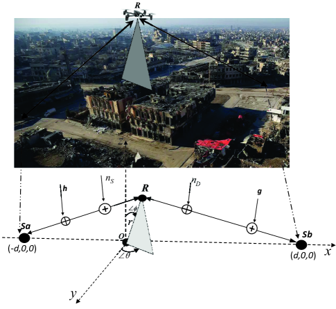
Figure 1: System Model

III Received signal at detestation node

This part derives an expression for the users $\mathit{SNRs}$ of the proposed UAV network. We first assume that the destination is entirely compensated by the Doppler effect due to the UAV’s mobility as the UAV follows a trajectory with a fixed flying speed [30]. Thereby, both flat fading channels $\mathit{S_{a}-R}$ and $\mathit{R-S_{b}}$ have power gains following the free-space path attenuation schemas $h\,d_{a}^{\frac{-\text{\textramshorns}}{2}}$and $g\,\,d_{b}^{\frac{-\text{\textramshorns}}{2}},$respectively, where $h$ is the channel coefficient between $S_{a}$ and $R$, $g$ is the channel coefficient between $S_{b}$ and $R$, is the path loss exponent which is commonly estimated in the range of $2\leq\text{\textramshorns}\leq 4$. It is also assumed that the channel’s characteristics are available at the user nodes. Further, user $S_{a}$ is able to adjust the transmit powers in $S_{b}$ and relay $\mathit{R}$. Similarly, $S_{a}$ can regulate $S_{a}$ and relay $\mathit{R}$ powers using the power allocation process.

A further assumption is that the users adopt binary phase shift keying modulation to broadcast their signals $\chi_{a}$ and $\chi_{b}$, with average power $p_{a}$ and $p_{b}$, from users $S_{a}$ and $S_{b}$, respectively. Both signals $\chi_{a}$ and $\chi_{b}$ are transmitted during the time interval $\mathit{0}<\mathit{t}\leq\mathcal{\mathcal{T}},$and each signal follows a circularly symmetric complex Gaussian distribution $\mathcal{CN}(0,1)$, i.e. $E\{\bigl{|}\chi_{a}\,\bigr{|}^{2}\}=1$ and $E\{\bigl{|}\chi_{b}\bigr{|}^{2}\}=1$, where $E\{.\}$ denotes an expected value and $\bigl{|}.\bigr{|}^{2}$ is the absolute square of a signal.

The $S_{a}$ and $S_{b}$ nodes transmit their bits according to a schedule that defines the commencing and the duration of each bit transmission. Then, $\chi_{a}$ and $\chi_{b}$ arrive to their target node in the time interval $\mathit{0}<\mathit{t}\leq\mathcal{\mathcal{T}}.$ In order to simplify, $\mathcal{T}$ is discretized into $n$ time slots as $\delta_{\mathit{t}}\mathcal{\mathrm{=}T}$/$\mathcal{N}$, where $\delta_{\mathit{t}}$ represents the time slot length. The value of $\delta_{\mathit{t}}$ is assumed to be small enough that the UAV’s location can be supposed to be approximately constant within a slot. Thereby, the UAV’s trajectory $\left(x_{i}\mathrm{(\mathit{t})},y_{i}\mathrm{(\mathit{t})},z_{i}\mathrm{(\mathit{t})}\right)$ over $\mathcal{T}$ can be specified by $\mathcal{N}$ scope as $\bigl{\{}x_{i}[n],y_{i}[n],z_{i}\mathrm{(\mathit{n})}\bigr{\}}_{n}^{\mathcal{N}}$ $\in\mathbb{R^{\mathrm{3}}},$where $\mathit{n=1,2,...\mathcal{N-\mathrm{1.}}}$

The exchange signals between $S_{a}$ and $S_{b}$ occur in two-hops. In the first hop, the relay receives signals from both $S_{a}$ and $S_{b}$ as

$$Y_{R}[n]=\sqrt{p_{a}\bigl{[}n\bigr{]}}\chi_{a}h+\sqrt{p_{b}\bigl{[}n\bigr{]}}\chi_{b\,}g\,d_{b}^{\frac{-\alpha}{2}}+\mathit{n}_{R},$$ (3)

where $h\,d_{a}^{\frac{-\alpha}{2}}$ and $g\,d_{b}^{\frac{-\alpha}{2}}$ are the fading channels model defined in [31], $n_{R}$ is the Gaussian noise of the relay with zero mean and variance $(\sigma^{2})$.

The $Y_{R}$ signal is then amplified by the relay amplification factor ($\beta$) given by:

$$\beta\bigl{[}n\bigr{]}=\sqrt{p_{R}\bigl{[}n\bigr{]}/(\left|h\right|^{2}d_{a}^{-\alpha}p_{a}\bigl{[}n\bigr{]}\,+\left|g\right|^{2}d_{b}^{-\alpha}p_{b}\bigl{[}n\bigr{]}+\sigma^{2}}),$$ (4)

where $p_{R}\bigl{[}n\bigr{]}$ is the allocated power for $R$ node .

After that, each user receives the amplified signals through the same flat fading channel, during the second time slot. The received signal by $S_{a}$ is then included in the relay-amplified signal beside the direct signal received from $S_{b}$ node. This gives

$$Y_{a}\bigl{[}n\bigr{]}=h\,d_{a}^{\frac{-\alpha}{2}}\beta\bigl{[}n\bigr{]}y_{R}+\sqrt{p_{b}}\chi_{b\,}g\,d_{b}^{\frac{-\alpha}{2}}$$

$$+2\sqrt{p_{b}}\chi_{b\,}gh\,\left|d\right|^{\frac{-\alpha}{2}}+n_{a}.$$ (5)

Node $S_{b}$ also involves the relay-amplified signal and the direct $S_{a}$ signal as the following

$$Y_{b}\bigl{[}n\bigr{]}=g\,d_{b}^{\frac{-\alpha}{2}}\beta\bigl{[}n\bigr{]}y_{R}+\sqrt{p_{a}}\chi_{a}\,h\,\,d_{a}^{\frac{-\alpha}{2}}$$

$$+2\sqrt{p_{a}}\chi_{a\,}gh\,\left|d\right|^{\frac{-\alpha}{2}}+n_{b},$$ (6)

where $gh$ is the channel coefficient between user $S_{a}$ and user $S_{b}$ with the separating distance 2$\left|d\right|,$and $n_{a}$ and $n_{b}$ are the users Gaussian noises with a zero mean and variance $(\sigma^{2})$ for both user $S_{a}$ and user $S_{b},$ respectively.

Equations (5) and (6) each have their own transmission signal mixed with the received signal and this is returned to self-interference (SI). Here, we assume that both users have an SI cancellation circuit that allows for their own transmitted signal to be cancelled out [32]. Thus, the SNRs at each user are given by

$$\gamma_{a}^{\iota} \bigl{[}n\bigr{]}=\frac{p_{R}\,\gamma_{b}\>p_{b}\,\gamma_{a}\,d_{b}^{-\alpha}d_{h}^{-\alpha}}{\gamma_{a}\>(p_{R}+p_{a})d_{a}^{-\alpha}+p_{b}\,\gamma_{b}d_{b}^{-\alpha}+1}+p_{R}p_{b}\gamma_{ab}\,d_{b}^{-\alpha},$$ (7)

$$\gamma_{b}^{\iota} \bigl{[}n\bigr{]}=\frac{p_{R}\,\gamma_{b}\>p_{a}\,\gamma_{a}\,d_{a}^{-\alpha}d_{b}^{-\alpha}}{p_{a}\,\gamma_{a}\>d_{a}^{-\alpha}+(p_{R}+p_{b})\,\gamma_{b}\,d_{b}^{-\alpha}+1}+p_{R}\,p_{a}\,\gamma_{ab}\,d_{a}^{-\alpha},$$ (8)

where $\gamma_{a}^{\iota}$ and $\gamma_{b}^{\iota}$ are the actual line-of-sight $\textit{$\mathit{SNR}$}s$ for $S_{a}$ and $S_{b}$, respectively, $\gamma_{ab}=\frac{\left|gh\right|^{2}}{\sigma^{2}},$ $\gamma_{a}=\frac{\left|h\right|^{2}}{\sigma^{2}}$ and $\gamma_{b}=\frac{\left|g\right|^{2}}{\sigma^{2}}.$

In the proposed UAV, the direct link between $S_{a}$ and user $S_{b}$ is usually not possible due to long-distance flight and degradation in channel quality. Therefore, the destination nodes receive only the relayed signals from the $R$ node, i.e., $\gamma_{ab}=0$. Equations (7) and (8) then become

$$\gamma_{a_{e}} \bigl{[}n\bigr{]}=\frac{p_{R}\,\gamma_{b}\>p_{b}\,\gamma_{a}\,d_{a}^{-\alpha}d_{b}^{-\alpha}}{\gamma_{a}\>(p_{R}+p_{a})d_{a}^{-\alpha}+p_{b}\,\gamma_{b}d_{b}^{-\alpha}+1},$$ (9)

$$\gamma_{b_{e}}\bigl{[}n\bigr{]} =\frac{p_{R}\,\gamma_{b}\>p_{a}\,\gamma_{a}\,d_{a}^{-\alpha}d_{b}^{-\alpha}}{p_{a}\,\gamma_{a}\>d_{a}^{-\alpha}+(p_{R}+p_{b})\,\gamma_{b}\,d_{b}^{-\alpha}+1},$$ (10)

where $\gamma_{a_{e}}$ and $\gamma_{b_{e}}$ are the exact non-line-of-sight SNRs for $S_{a}$ and $S_{b}$, respectively

The average power $\overline{p}_{r}$, $\overline{p}_{a}$ and $\overline{p}_{b}$ should not exceed the overall network power $(\overline{P})$ $\left\{\overline{P}:\overline{P}\in\mathbb{R},\overline{P}=\underset{i}{\sum}\overline{p}_{i}\quad i\in\left(a,r,b\right)\right\}$. In order to manage $\overline{P}$ value, the power allocation strategy is used to allocate a specific power value to the relay and both user nodes. All nodes have inclusive knowledge of information about channels and maximum transmission power for each related node [33], so both $S_{a}$ and $S_{b}$ nodes achieve the allocation strategy by employing the reverse channels for feedback allocated energy factors to the corresponding node. After that, $S_{a}$, $S_{b}$ and relay nodes adjust their transmit power based on these feedback factors [34].

It assumes that the energy allocation factors $S_{a}$, $\mathit{R}$ and $S_{b}$, respectively, are set as

$$\alpha_{a}\Rightarrow\left\{\alpha_{a}:\in\mathbb{R\mathit{,}}\rightarrow 0\leq\alpha_{a}\leq 1\right\},$$ (11)

$$\alpha_{r}\Rightarrow\left\{\alpha_{r}:\in\mathbb{R\mathit{,}}\rightarrow 0\leq\alpha_{r}\leq 1\right\},$$ (12)

$$\alpha_{b}\Rightarrow\left\{\alpha_{b}:\in\mathbb{R\mathit{,}}\rightarrow 0\leq\alpha_{b}\leq 1\right\}.$$ (13)

Once received, the corresponding nodes adjust their powers as $\overline{P}\>\alpha_{b},\overline{P}\>\alpha_{r}$ and $\overline{P}\>\alpha_{a}$. So, substituting these regulated powers into (9) and (10) and considering high $\mathit{SNR}$ domain, we get

$$\gamma_{a}[n]=\overline{P}\frac{\alpha_{r}\>\bigl{[}n\bigr{]}\,\gamma_{b}\>\alpha_{b}\bigl{[}n\bigr{]}\,\gamma_{a}d_{a}^{-\text{\textramshorns}}d_{b}^{-\text{\textramshorns}}}{\gamma_{a}\>(\alpha_{r}\>\bigl{[}n\bigr{]}\,+\alpha_{a}\>\bigl{[}n\bigr{]}\,)d_{a}^{-\text{\textramshorns}}+\alpha_{b}\bigl{[}n\bigr{]}\,\gamma_{b}d_{b}^{-\text{\textramshorns}}},$$ (14)

$$\gamma_{b}[n]=\overline{P}\frac{\alpha_{r}\>\bigl{[}n\bigr{]}\,\,\gamma_{b}\>\alpha_{a}\>\bigl{[}n\bigr{]}\,\,\gamma_{a}d_{a}^{-\text{\textramshorns}}d_{b}^{-\text{\textramshorns}}}{\alpha_{a}\>\bigl{[}n\bigr{]}\,\,\gamma_{a}\>d_{a}^{-\text{\textramshorns}}+(\alpha_{r}\>\bigl{[}n\bigr{]}\,+\alpha_{b}\>\bigl{[}n\bigr{]}\,)\,\gamma_{b}d_{b}^{-\text{\textramshorns}}},$$ (15)

where $\gamma_{a}$ and $\gamma_{b}$ are the high SNRs domain for (9) and (10), respectively

Now, another metric is the channel capacity, which is given by

$$C[n]=\frac{1}{2}\log_{2}(1+\phi[n]).\;\quad bits/s,$$ (16)

where $\phi[n]=1+\gamma_{a}[n]+\gamma_{b}[n]+\gamma_{a}[n]\gamma_{b}[n].$

To adapt reliably transmitted information rate ($\mathcal{R}$), we have

$$\mathcal{R}[\mathit{n}]=\mathfrak{h}\>C[n]\;\left(0<\text{\text{$\mathfrak{h}$}}<1\right)$$ (17)

At $\text{\text{$\mathfrak{h}$}}=1,$the maximum data rate in (16) becomes

$$\Re_{i}=\Re_{a}+\Re_{b}=\frac{1}{2}\left(\log_{2}(1+\gamma_{a}[n])+\log_{2}(1+\gamma_{b}[n])\right),$$ (18)

where $\Re_{i}$ is the total data rate in two way [35].

As mentioned earlier, the data rate $\mathcal{R}[\mathit{n}]$ is passed through two hops, i.e., two cascade channels. The transmission rate through two channels is subjected to an Information Cascade (IC) analysis [36], which is defined as a propagation sequence of data bits transmitting over chaotic channels. Further, the mutual-information flow along the cascade of channels cannot exceed each channel individually. Along the cascade channels, the flow mutual information capacity cannot overpass each channel capacity. Regarding UAV channels, the first channel delivers a sequence of bits that transmitted by users nodes to the $\mathit{R}$ node during a time slot $\mathit{n=\mathrm{1}.}$ The $\mathit{R}$ node requires one-slot processing to forward the received data to the $S_{a}$ and $S_{b}$ node during the second time slots, i.e. $\mathit{n}$= 2, 3, 4,…$\mathcal{N}$ [37]. Then, the information-causality constrain is obtained as:

$$\underset{\begin{gathered}S_{a}\rightarrow R\rightarrow S_{b}\\ S_{b}\rightarrow R\rightarrow S_{a}\end{gathered}}{\underbrace{\sum_{\mathrm{i=2}}^{\mathrm{n}}\overline{R}\mathrm{[\mathit{i}]}}}\leq\underset{\begin{gathered}R\rightarrow S_{a}\\ R\rightarrow S_{b}\end{gathered}}{\underbrace{\sum_{\mathrm{i=1}}^{\mathrm{n-1}}\overline{R}\mathrm{[\mathit{i}]}}}.$$ (19)

$S_{a}\rightarrow R\rightarrow S_{b}$ and $S_{b}\rightarrow R\rightarrow S_{a}$ represent the transmitted a signal from $S_{a}$ to $S_{b}$ and from $S_{b}$ to $S_{a}$, respectively, $R\rightarrow S_{a}$ and $R\rightarrow S_{b}$ typify the amplified signal forwarded by $\mathit{R}$ to $S_{a}$ and $S_{b}$ through one channel.

Input: $\overline{P},\textit{x(t)},\alpha_{a},\alpha_{b},\text{and }\alpha_{r}$

Initialization of parameters

while $t\neq 0$ do

      $d_{a}\leftarrow\eqref{eq: d1}$

       $d_{b}\leftarrow\eqref{eq: d2}$

       $\gamma_{a}\leftarrow E{Y_{a}[n]}$ $\triangleright$ expectation value of (9)

       $\gamma_{a}\leftarrow E{Y_{b}[n]}$ $\triangleright$ expectation value of (10) $p_{a}=\overline{P}\>\alpha_{a}$ ; $p_{b}=\overline{P}\>\alpha_{b}$; $p_{r}=\overline{P}\>\alpha_{r}$

       $\gamma_{a}\leftarrow\eqref{eq:Hi-SNR a}$

       $\gamma_{b}\leftarrow\eqref{eq:HI-SNR b}$

end while

Output: $\mathit{SNR}$

Algorithm 1 Procedure of $\mathit{SNR}$ analysis

IV Energy Allocation

This section will concentrate on an energy allocation problem to manage energy consumption in the users and relay nodes of UAV networks. Energy consumption is related to transmission delay [38], so the proposed energy allocation allows total energy consumption and data transmission time (delay) to be minimised under a balanced approach.

In Shannon’s theorem, prolonging the transmission time reduces transmitting power. Thus, the total energy consumption in UAV networks is minimised by maximising transmission time. However, increasing transmission delay in transmitting the information directly affects the user’s service. Hence, transmission time $(q)$ and power networks must be designed with a trade-off scheme. $\mathit{q}$ is the amount of time required by a user to send out a single packet of bits; it depends on the network’s bandwidth and length of the packet, as $q$ = (Data size/bandwidth) (sec). By using low-latency algorithms or low-delay transmission protocols, data transmission amounts can be adjusted, and delays can be reduced. Such approaches allow the data transmission amount to be managed according to the change in delay performance due to a change in transmission amount. Each data bit delivered at $\mathit{q}$ can consume energy ($\mathcal{E})$ as $\mathcal{E}=q\>P$. Then, the total energy model in UAV is defined from (14), (15) and (17) as follows

$$\mathcal{E}_{\mathit{a}}\bigl{[}n\bigr{]}=q[n]\left(\>(\alpha_{r}\>\bigl{[}n\bigr{]}\,+\alpha_{a}\>\bigl{[}n\bigr{]}\,)H+\alpha_{b}\bigl{[}n\bigr{]}\,G\right)\left(2^{\frac{2}{q[n]}}-1\right),$$ (20)

$$\mathcal{\mathcal{E}_{\mathit{b}}}\bigl{[}n\bigr{]}=q[n]\left(\alpha_{a}\>\bigl{[}n\bigr{]}\,\,H+(\alpha_{r}\>\bigl{[}n\bigr{]}\,+\alpha_{b}\>\bigl{[}n\bigr{]}\,)\,G\right)\left(2^{\frac{2}{q[n]}}-1\right),$$ (21)

where $G=\gamma_{b}d_{b}^{-\text{\textramshorns}}$, $H=\gamma_{a}d_{a}^{-\text{\textramshorns}}$.

Concurrent with the information exchanging between $S_{a}$ and $S_{b},$ the overall energy consumption is typically generated by including (20) and (21), i.e., $\,\mathcal{E}\bigl{[}n\bigr{]}=\,\mathcal{E}_{\mathit{a}}\bigl{[}n\bigr{]}+\mathcal{\mathcal{E}_{\mathit{b}}}\bigl{[}n\bigr{]}$, as in [2]. The region $\mathcal{E}\bigl{[}n\bigr{]}$ can also be specified by the union of all the possible sets of $\left(\mathcal{E}_{\mathit{a}},\mathcal{E}_{\mathit{b}}\right),$ as in [30]. Hence, if the region $\mathcal{E}\bigl{[}n\bigr{]}$ is managed by varying $\alpha_{a},\alpha_{b},\alpha_{r},$then the union of the two sets of energies in (20) and (21) are subject to definition 1.

Definition 1. The regions of two sets $\,\mathcal{E}_{\mathit{a}}$ and $\,\mathcal{E}_{\mathit{b}}$ is the collection of all objects that are in either set. Then, the union of $\,\mathcal{E}_{\mathit{a}}$ and $\,\mathcal{E}_{\mathit{b}}$ is defined as: $\,\bigcup\mathcal{E}_{i}\bigl{[}n\bigr{]}=\mathcal{\,E}_{\mathit{a}}\cup\mathcal{\,E}_{\mathit{b}}\left\{\alpha_{i}:\left(\alpha_{i}\in\mathcal{\,E}_{\mathit{a}}\right)\lor\left(\alpha_{i}\in\mathcal{\,E}_{\mathit{a}}\right)\right\}$$\quad i\in\left\{a,\,b,r\right\}$.

Now, the total energy consumption can be expressed in regard to $\alpha_{i}$ as the following

$$\,\mathcal{E}_{i}(\alpha_{i})\bigl{[}n\bigr{]}=\,\mathcal{E}_{\mathit{a}}\bigl{[}n\bigr{]}+\mathcal{\mathcal{E}_{\mathit{b}}}\bigl{[}n\bigr{]}\quad\quad i\in\left\{a,b,r\right\}.$$ (22)

For each transmitted bit, the value of $q$ can be defined as $q\bigl{[}n\bigr{]}=1/\mathcal{R}[n]$, so from (17) we have

$$\mathit{q_{a}}(\alpha_{i})[\mathit{n}]=2\>\log_{2}\left(1+\,G\overline{P}\frac{\alpha_{r}\>\alpha_{b}}{\alpha_{r}+\alpha_{a}\>+\alpha_{b}\,\frac{G}{H}}\right)^{-1},$$ (23)

$$\mathit{q_{b}}(\alpha_{i})[\mathit{n}]=2\>\log_{2}\left(1+\>G\overline{P}\frac{\alpha_{r}\>\alpha_{a}}{\alpha_{a}\>+(\alpha_{r}\,+\alpha_{b}\,)\frac{G}{H}}\right)^{-1}i\in\left\{a,\,b,r\right\},$$ (24)

where (.)^-1 indicates reciprocal action.

In two-way relay networks, the powers design of relay and users nodes are defined as $\left(p_{a}[n]+p_{r}[n]+p_{b}[n]\right)\leq P\bigl{[}n]$ [32]. In this case, the proposed allocated power is expressed considering (19) as

$$\underset{\mathrm{\mathit{\begin{gathered}\mathrm{the\;}\mathrm{total\>transmit\;power\;of}\\ \mathrm{two\;hops}\end{gathered}}}}{\underbrace{\sum_{\mathrm{\mathit{\mathrm{n=2}}}}^{\mathit{\mathcal{N}}}\left(p_{a}[n]+p_{r}[n]+p_{b}[n]\right)}}\leq P\bigl{[}n\bigr{]}.$$ (25)

The purpose of this paper is to optimize $\alpha_{i}$ i.e., $\alpha_{a},\alpha_{b}$ and $\alpha_{\mathit{r}}$ in order to regulate the energy consumption of (20) and (21) and the transmission delay of (23) and (24) in a balanced way. Hence, the optimisation problem can be formulated as follows

$$\mathcal{\mathrm{min}\>\>E}_{a}(\alpha_{i})[n],$$ (26)

$$\mathcal{\mathrm{min}\>\>E}_{b}(\alpha_{i})[n],$$ (27)

$$\mathit{\mathcal{\mathrm{min}\>\>}}\left(q_{a}(\alpha_{i}[\mathit{n}]\mathit{+q_{b}}(\alpha_{i})[\mathit{n}]\right),$$ (28)

$$s.t\qquad\forall n\quad\alpha_{a}[\mathit{n}]+\alpha_{b}[\mathit{n}]+\alpha_{r}[\mathit{n}]\leq 1.$$ (29)

All objectives (26)-(28) must be minimized at once under the constraint of (29); however, the issue is that both (26) and (27) are in contras to (28). Multi-objective optimisation techniques, particularly the weight scalarization method [7], are some of the most reliable methods for resolving such an issue. In the weight scalarization method, all of the objective functions are consolidated into a single function that appears as a linear function. Many studies have adopted the scalarization approach to optimise different mathematical functions such as quadratic and logarithmic functions. By employing the scalarization approach to minimise (26)-(28) under constraint (29), the following expression is obtained

$$F(\alpha_{a},\alpha_{\mathit{b}},\alpha_{r},w)[n]=\sum_{\mathrm{\mathit{\mathrm{n=2}}}}^{\mathit{\mathcal{N}}}\left(w_{a}\mathcal{\>E}_{a}(\alpha_{i})[n]+w_{b}\mathcal{\>E}_{a}(\alpha_{i})[n]\right.$$

$$\left.+w_{r}\>\left(\mathit{q_{a}}(\alpha_{i})[\mathit{n}]+\mathit{q_{b}}(\alpha_{i})[\mathit{n}]\right)\right)\quad\quad\forall n,$$ (30)

where $w_{a}\left\{w_{a}:\,\in\mathbb{R},\;0<w_{a}\leq 1\right\}$, $w_{b}\left\{w_{b}:\,\in\mathbb{R},\;0<w_{b}\leq 1\right\}$ and $w_{r}\left\{w_{r}:\,\in\mathbb{R},\;0<w_{r}\leq 1\right\}.$

The weight coefficients are limited to the following constraint: $\sum_{\mathrm{\mathit{i}}}^{\mathit{m}}w_{i}\leq 1,$where $\mathit{m}$ is the number of functions and $i\in\left\{a,b,r\right\}.$ Equation (30) reveals that both $\mathit{q_{a}}(\alpha_{i})[\mathit{n}]$ and $\mathit{q_{b}}(\alpha_{i})[\mathit{n}]$ express as linear with a single weight coefficient; this is because the proposed system model assumes that $S_{a}$ and $S_{b}$, are exchanging information simultaneously with each other through $\mathit{R}.$

The minimum solution of the objective function $F(\alpha_{a},\alpha_{\mathit{b}},\alpha_{r},w)$ is obtained by satisfying the conditions $\begin{bmatrix}{\normalcolor\frac{\partial\left(\alpha_{a},\alpha_{\mathit{b}},\alpha_{r},w\right)}{\partial\alpha_{a}}}&{\normalcolor\frac{\partial\left(\alpha_{a},\alpha_{\mathit{b}},\alpha_{r},w\right)}{\partial\alpha_{b}}}&{\normalcolor\frac{\partial\left(\alpha_{a},\alpha_{\mathit{b}},\alpha_{r},w\right)}{\partial\alpha_{r}}}\end{bmatrix}^{\mathrm{T}}=0$ and $\begin{bmatrix}{\normalcolor\frac{\partial\left(\alpha_{a},\alpha_{\mathit{b}},\alpha_{r},w\right)}{\partial\alpha_{a}\alpha_{b}}}&{\normalcolor\frac{\partial\left(\alpha_{a},\alpha_{\mathit{b}},\alpha_{r},w\right)}{\partial\alpha_{b}\alpha_{r}}}&{\normalcolor\frac{\partial\left(\alpha_{a},\alpha_{\mathit{b}},\alpha_{r},w\right)}{\partial\alpha_{r}\alpha_{a}}}\end{bmatrix}^{\mathrm{T}}>0$. Thus, it is required to calculate the following equations

$$\frac{\partial F(\alpha_{a},\alpha_{\mathit{b}},\alpha_{r},w)}{\partial\alpha_{a}}=q[n]\;H\;\left(2^{\frac{2}{q[n]}}-1\right)\left(w_{a}+w_{b}\right)$$

$$-w_{r}G\overline{P}\left(\frac{\alpha_{b}H^{2}\alpha_{r}}{\left(\alpha_{b}G+H\alpha_{r}+H\alpha_{a}\right)^{2}}+\frac{GH\alpha_{r}(\alpha_{b}+\alpha_{r})}{\left(\alpha_{b}G+G\alpha_{r}+H\alpha_{a}\right)^{2}}\right).$$ (31)

$$\frac{\partial F(\alpha_{a},\alpha_{\mathit{b}},\alpha_{r},w)}{\partial\alpha_{b}}=q[n]\;G\;\left(2^{\frac{2}{q[n]}}-1\right)\left(w_{a}+w_{b}\right)$$

$$+w_{r}G\overline{P}\left(\frac{H^{2}\alpha_{r}(\alpha_{a}+\alpha_{r})}{\left(\alpha_{b}G+H\alpha_{r}+H\alpha_{a}\right)^{2}}-\frac{\alpha_{a}GH\alpha_{r}}{\left(\alpha_{b}G+G\alpha_{r}+H\alpha_{a}\right)^{2}}\right),$$ (32)

$$\frac{\partial F(\alpha_{a},\alpha_{\mathit{b}},\alpha_{r},w)}{\partial r}=q[n]\;H\;\left(2^{\frac{2}{q[n]}}-1\right)\left(H\,w_{a}+G\,w_{b}\right)$$

$$+w_{r}G\overline{P}\left(\frac{\alpha_{b}H(\alpha_{a}H+\alpha_{b}G)}{\left(\alpha_{b}G+H\alpha_{r}+H\alpha_{a}\right)^{2}}+\frac{\alpha_{a}H(\alpha_{a}H+\alpha_{b}G)}{\left(\alpha_{b}G+G\alpha_{r}+H\alpha_{a}\right)^{2}}\right).$$ (33)

Also we have

$$\begin{bmatrix}{\normalcolor\frac{\partial\left(\alpha_{a},\alpha_{\mathit{b}},\alpha_{r},w\right)}{\partial\alpha_{a}\alpha_{b}}}\\ {\normalcolor\frac{\partial\left(\alpha_{a},\alpha_{\mathit{b}},\alpha_{r},w\right)}{\partial\alpha_{b}\alpha_{r}}}\\ {\normalcolor\frac{\partial\left(\alpha_{a},\alpha_{\mathit{b}},\alpha_{r},w\right)}{\partial\alpha_{r}\alpha_{a}}}\end{bmatrix}=$$

$$\begin{bmatrix}\frac{-H^{2}r(\alpha_{a}H-G\alpha_{b}+H\alpha_{r})G\overline{P}}{(\alpha_{a}H+G\alpha_{b}+H\alpha_{r})^{3}}&\frac{GHr(\alpha_{a}H-G(\alpha_{r}+\alpha_{b}))G\overline{P}}{(\alpha_{a}H+G(\alpha_{r}+\alpha_{b}))^{3}}\\ \frac{G\overline{P}H^{2}\left(\alpha_{a}^{2}H+\alpha_{a}bG+aH\alpha_{r}+2\alpha_{b}G\alpha_{r}\right)}{(H(\alpha_{a}+\alpha_{r})+\alpha_{b}G)^{3}}&\frac{-\alpha_{a}GH(\alpha_{a}H+\alpha_{b}G-G\alpha_{r})G\overline{P}}{(\alpha_{a}H+\alpha_{b}G+G\alpha_{r})^{3}}\\ \frac{\alpha_{b}H^{2}(\alpha_{b}G+H(\alpha_{a}-\alpha_{r}))G\overline{P}}{(\alpha_{b}G+H(\alpha_{r}+\alpha_{a}))^{3}}&\frac{2\alpha_{a}H^{2}(\alpha_{a}H+\alpha_{b}G)G\overline{P}}{(\alpha_{b}G+G\alpha_{r}+H\alpha_{a})^{3}}\end{bmatrix}.$$ (34)

Equation (34) illustrates that the second partial derivative test $\begin{bmatrix}{\normalcolor\frac{\partial\left(\alpha_{a},\alpha_{\mathit{b}},\alpha_{r},w\right)}{\partial\alpha_{a}\alpha_{b}}}&{\normalcolor\frac{\partial\left(\alpha_{a},\alpha_{\mathit{b}},\alpha_{r},w\right)}{\partial\alpha_{b}\alpha_{r}}}&{\normalcolor\frac{\partial\left(\alpha_{a},\alpha_{\mathit{b}},\alpha_{r},w\right)}{\partial\alpha_{r}\alpha_{a}}}\end{bmatrix}^{\mathrm{T}}>0$. Thus, the minimum local points of equations (31) to (33) are obtained after setting the first conditions, i.e., $\frac{\partial F(\alpha_{a},\alpha_{\mathit{b}},\alpha_{r},w)}{\partial\alpha_{a}}=0$, $\frac{\partial F(\alpha_{a},\alpha_{\mathit{b}},\alpha_{r},w)}{\partial\alpha_{b}}=0$ and $\frac{\partial F(\alpha_{a},\alpha_{\mathit{b}},\alpha_{r},w)}{\partial\alpha_{r}}=0$.

Before continuing with this analysis, another test should be applied to $F\mathit{\mathrm{[}n}\bigr{]}(\alpha_{a},\alpha_{\mathit{b}},\alpha_{r})$. This test aims to find whether the $F$ function is a convex function or not, as the weigh scalarization method is inefficient to find a solution with a non-convex function [39]. To achieve such a test, the Bordered Hessian ($\mathit{H_{b}}$) matrix is employed as follows:

$$\mathtt{z}^{\mathtt{T}}\mathit{H_{b}}\mathtt{z}=\begin{bmatrix}\mathtt{z_{1}}&\mathtt{z_{2}}&\mathtt{z_{3}}&\mathtt{z_{4}}\end{bmatrix}$$

$$\left[\begin{array}[]{ccc}0&\frac{\partial F\left(\alpha_{a},\alpha_{\mathit{b}},\alpha_{r},w\right)}{\partial\alpha_{a}}&\frac{\partial F\left(\alpha_{a},\alpha_{\mathit{b}},\alpha_{r},w\right)}{\partial\alpha_{b}}\\ \frac{\partial F(\alpha_{a},\alpha_{\mathit{b}},\alpha_{r},w)}{\partial\alpha_{a}}&\frac{\partial^{2}F(\alpha_{a},\alpha_{\mathit{b}},\alpha_{r},w)}{\partial\alpha_{a}^{2}}&\frac{\partial F^{2}(\alpha_{a},\alpha_{\mathit{b}},\alpha_{r},w)^{2}}{\partial\alpha_{a}\partial\alpha_{b}}\\ \frac{\partial F(\alpha_{a},\alpha_{\mathit{b}},\alpha_{r},w)}{\partial\alpha_{b}}&\frac{\partial^{2}F(\alpha_{a},\alpha_{\mathit{b}},\alpha_{r},w)}{\partial\alpha_{a}\partial\alpha_{b}}&\frac{\partial^{2}F(\alpha_{a},\alpha_{\mathit{b}},\alpha_{r},w)}{\partial\alpha_{b}^{2}}\\ \frac{\partial F(\alpha_{a},\alpha_{\mathit{b}},\alpha_{r},w)}{\partial\alpha_{r}}&\frac{\partial^{2}F(\alpha_{a},\alpha_{\mathit{b}},\alpha_{r},w)}{\partial\alpha_{a}\partial\alpha_{r}}&\frac{\partial^{2}F(\alpha_{a},\alpha_{\mathit{b}},\alpha_{r},w)}{\partial\alpha_{b}\partial\alpha_{r}}\end{array}\right.$$ (39)

$$\left.\begin{array}[]{c}\frac{\partial F\left(\alpha_{a},\alpha_{\mathit{b}},\alpha_{r},w\right)}{\partial\alpha_{r}}\\ \frac{\partial^{2}F(\alpha_{a},\alpha_{\mathit{b}},\alpha_{r},w)}{\partial\alpha_{a}\partial\alpha_{r}}\\ \frac{\partial^{2}F(\alpha_{a},\alpha_{\mathit{b}},\alpha_{r},w)}{\partial\alpha_{b}\partial\alpha_{r}}\\ \frac{\partial^{2}F(\alpha_{a},\alpha_{\mathit{b}},\alpha_{r},w)}{\partial\alpha_{r}^{2}}\end{array}\right]\begin{bmatrix}\mathtt{z_{1}}\\ \mathtt{z_{2}}\\ \mathtt{z_{3}}\\ \mathtt{z_{4}}\end{bmatrix}.$$ (44)

Substituting (31)-(34) into (44) leads to the following results: $\mathtt{z}^{\mathtt{T}}\mathit{H_{b}}\mathtt{z}\geq 0$, i.e., $\mathit{H_{b}}$ is non-negative. Therefore, the Hessian matrix is positive semidefinite; hence $F(\alpha_{a},\alpha_{\mathit{b}},\alpha_{r},w)$ is a set of convex.

Now, we evaluate $\begin{bmatrix}{\normalcolor\frac{\partial\left(\alpha_{a},\alpha_{\mathit{b}},\alpha_{r},w\right)}{\partial\alpha_{a}}}&{\normalcolor\frac{\partial\left(\alpha_{a},\alpha_{\mathit{b}},\alpha_{r},w\right)}{\partial\alpha_{b}}}&{\normalcolor\frac{\partial\left(\alpha_{a},\alpha_{\mathit{b}},\alpha_{r},w\right)}{\partial\alpha_{r}}}\end{bmatrix}^{\mathrm{T}}=0$ from (31) to (33). This gives

$$\overset{*}{\alpha}_{a}(w_{j})=\frac{1}{\psi_{a}}\left(\psi_{b}\pm\sqrt{\psi_{b}^{2}+2\psi_{a}\psi_{c}}\right)\quad\forall n,$$ (45)

$$\overset{*}{\alpha}_{\mathit{b}}(w_{j})=\left(\frac{1}{\psi_{a}}\left(\psi_{b}\pm\sqrt{\psi_{b}^{2}+2\psi_{a}\psi_{c}}\right)\left(\frac{H}{G}-1\right)+1\right)$$

$$\sqrt{\frac{q\left(2^{\frac{2}{q[n]}}-1\right)\left[\;H-G\right]}{2HG\overline{P}\left(w_{3}\right)}\left(1-w_{3}\right)}\quad\forall n,$$ (46)

$$\overset{*}{\alpha}_{\mathit{r}}(w_{j})=1-\frac{1}{\psi_{a}}\left(\psi_{b}\pm\sqrt{\psi_{b}^{2}+2\psi_{a}\psi_{c}}\right)$$

$$-\left(\frac{1}{\psi_{a}}\left(\psi_{b}\pm\sqrt{\psi_{b}^{2}+2\psi_{a}\psi_{c}}\right)\left(\frac{H}{G}-1\right)+1\right)$$

$$\sqrt{\frac{q\left(2^{\frac{2}{q[n]}}-1\right)\left[\;H-G\right]}{2HG\overline{P}\left(w_{3}\right)}\left(1-w_{3}\right)}\quad\forall n,$$ (47)

where $(w_{j}):j\in\left\{a\vee\,b,r\right\}$, $\vee$ is ’or’ symbol, $\psi_{a}=2\left(G-H\right)$

$$\left(\mathrm{1}-\left(\frac{q\left(2^{\frac{2}{q[n]}}-1\right)\left[H-G\right]\left(w_{2}\right)}{2HG\overline{P}\left(w_{3}\right)}-\frac{1}{\left(G-H\right)+H}\right)\mathrm{(G-H)}\right)$$ ,

$\psi_{b}={\color[rgb]{0,0,0}\left(\frac{H}{G}-1\right)}\sqrt{G\frac{q\left(2^{\frac{2}{q[n]}}-1\right)\left[\;H-G\right]}{2H\overline{P}\left(w_{3}\right)}\left(1-w_{3}\right)}$+2G and $\psi_{c}=\sqrt{G\frac{q\left(2^{\frac{2}{q[n]}}-1\right)\left[\;H-G\right]}{2H\overline{P}\left(w_{3}\right)}\left(1-w_{3}\right)}-G$.

The solution of (45)-(47) depend on any variation of two-weight coefficient, and this gives an expected result because the proposed system model has two sources, $S_{a}$ and $S_{b}$, and both sources contribute to adjusting the energy allocation parameters. Based on several $w_{j}$, (45)-(47) provide a trade-off between energy consumption and transmission time. This agrees with the analysis in [40], which demonstrated that the weight scalarization method produce trade-off solution by repeating the analysis process for several weight coefficients.

Thus, the solution (28) is obtained by using (45)-(47) as follows:

$$\overset{*}{q_{i}}\bigl{[}n\bigr{]}(w_{j})=2/\left(1+\log_{2}\left(1+\varPhi\bigl{[}n\bigr{]}\right)\right).$$ (48)

By adding (26) and (27) together, the total energy consumption solution is calculated in terms of (45)-(47) as follows:

$$\mathcal{\mathcal{\overset{*}{E}}}_{i}\bigl{[}n\bigr{]}(w_{j})=\overset{*}{q_{i}}\bigl{[}n\bigr{]}\left(2^{\frac{2}{q[n]}}-1\right)\left(\left(\overset{*}{\alpha}_{\mathit{r}}(w_{j})\,+2\overset{*}{\alpha}_{a}(w_{j})\right)H\right.$$

$$\left.+\left(\overset{*}{\alpha}_{\mathit{r}}(w_{j})+2\overset{*}{\alpha}_{\mathit{b}}(w_{j})\right)\,G\right)\quad j\in\left\{a\,\vee\,b,r\right\},$$ (49)

where, $\varPhi\bigl{[}n\bigr{]}=1+\log_{2}\left(1+\,G\overline{P}\frac{\overset{*}{\alpha}_{\mathit{r}}(w_{j})\>\overset{*}{\alpha}_{\mathit{b}}(w_{j})}{\overset{*}{\alpha}_{\mathit{r}}(w_{j})+\overset{*}{\alpha}_{a}(w_{j})+\overset{*}{\alpha}_{\mathit{b}}(w_{j})\,\frac{G}{H}}\right)$

$+\log_{2}\left(1+\,G\overline{P}\frac{\overset{*}{\alpha}_{\mathit{r}}(w_{j})\overset{*}{\alpha}_{\mathit{b}}(w_{j})}{\overset{*}{\alpha}_{\mathit{r}}(w_{j})+\overset{*}{\alpha}_{a}(w_{j})+\overset{*}{\alpha}_{\mathit{b}}(w_{j})\,\frac{G}{H}}\right)$ $\left(1+\>G\overline{P}\frac{\overset{*}{\alpha}_{\mathit{r}}(w_{j})\>\overset{*}{\alpha}_{a}(w_{j})}{\overset{*}{\alpha}_{a}(w_{j})+(\overset{*}{\alpha}_{\mathit{r}}(w_{j})+\overset{*}{\alpha}_{\mathit{b}}(w_{j}))\frac{G}{H}}\right)$

$+\log_{2}\left(1+\>G\overline{P}\frac{\overset{*}{\alpha}_{\mathit{r}}(w_{j})\>\overset{*}{\alpha}_{a}(w_{j})}{\overset{*}{\alpha}_{a}(w_{j})+(\overset{*}{\alpha}_{\mathit{r}}(w_{j})+\overset{*}{\alpha}_{\mathit{b}}(w_{j}))\frac{G}{H}}\right).$

The (48) and (49) procedures are listed in Algorithm 2.

Input: ${\gamma_{a},\text{and }\gamma_{b}}$

Initialization of parameters

while $t\neq 0$ do

      $\mathcal{R}\leftarrow\eqref{eq: R-rate}$

       $\mathcal{E}_{a}(\alpha_{a},\alpha_{b},\alpha_{r})\leftarrow\eqref{eq: Ea}$

       $\mathcal{E}_{b}(\alpha_{b},\alpha_{b},\alpha_{r})\leftarrow\eqref{eq: Eb}$

       $\mathit{q}_{a}(\alpha_{a},\alpha_{b},\alpha_{r})\leftarrow\eqref{eq: qa}$

       $\mathit{q}_{b}(\alpha_{a},\alpha_{b},\alpha_{r})\leftarrow\eqref{eq: qb}$

       for $w_{i}=0:$ to $1$ do

             for $w_{j}=0:$ to $1$ do

                  

                  $F(\alpha_{a},\alpha_{b},\alpha_{r},w_{i,j})\leftarrow\eqref{eq: 1G-Form-1}$

                   $\overset{*}{\alpha_{a}}(w_{i,j})\leftarrow\eqref{eq:opt-Alph-A}$

                   $\overset{*}{\alpha_{b}}(w_{i,j})\leftarrow\eqref{eq:opt-Alph-B}$

                   $\overset{*}{\alpha_{r}}(w_{i,j})\leftarrow\eqref{eq:opt-Alph-r}$

                   $\overset{*}{\mathit{q}_{i}}(\overset{*}{\alpha_{a}},\overset{*}{\alpha_{b}},\overset{*}{\alpha_{r}})\leftarrow\eqref{eq: opt_qt}$

                   $\overset{*}{\mathcal{E}_{i}}(\overset{*}{\alpha_{a}},\overset{*}{\alpha_{b}}\overset{*}{\alpha_{r}})\leftarrow\eqref{eq: Opt-Ei}$

                  

             end for

            

       end for

      

end while

Output: $\mathcal{E}_{a}(\alpha_{a},\alpha_{b},\alpha_{r})$;$\mathcal{E}_{b}(\alpha_{b},\alpha_{b},\alpha_{r})$; $\mathit{q}_{a}(\alpha_{b},\alpha_{b},\alpha_{r})$;$\mathit{q}_{b}(\alpha_{b},\alpha_{b},\alpha_{r})$

Algorithm 2 Proposed energy-delay trade-off

V Bit error rate performance

This section discusses the optimum bit error rate ($\overset{*}{\text{\texthtb}_{e}}$) behaviour of the UAV network based on Equation (49). The bit error metric defines the number of errors that occur during data transmission on the UAV network. It can be reformatted for each transmitted bit (i.e. $\mathcal{\overline{R}}=1)$ as follows

$$\frac{1}{\overset{*}{\gamma}(w_{j})[n]}=\frac{1}{\left(\left(\overset{*}{\alpha}_{\mathit{r}}(w_{j})\,+2\overset{*}{\alpha}_{a}(w_{j})\right)H\overline{P}\right.}+\,\frac{1}{\left(\overset{*}{\alpha}_{\mathit{r}}(w_{j})+2\overset{*}{\alpha}_{\mathit{b}}(w_{j})\right)\overline{P}G},$$ (50)

where $\overset{*}{\gamma}(w_{j})$ the optimal SNR.

Equation (50) reveals that the $\mathit{SNR}$ is increasing function of optimal allocation factor $(\varphi_{i}),$ $\varphi_{i}\in\left(\overset{*}{\alpha_{a}}(w_{j}),\overset{*}{\alpha}_{b}(w_{j}),\overset{*}{\alpha}_{r}(w_{j})\right)$. Further, according to [41], bit error rate decreases when the overall received SNR is maximised. Thus, increasing $\varphi_{i}$ in (50) allows bit error rate to be minimised as demonstrate in the following analysis.

In the proposed UAV network, the transmitted signal from a $\mathit{S_{a}}$ to the $\mathit{\mathit{S_{b}}}$ node propagates through two cascaded channels, as illustrated in (1). Each channel is a Rayleigh fading and, in such a link, SNR follows a negative exponential distribution. Then the total SNR obtained from two i.i.d channels follows a negative exponential distribution. To find the total probability density function (pdf) of the $\mathit{S_{a}-R}$ and $\mathit{R-S_{b}}$ channels, distribution of the harmonic mean of two i.i.d. gamma random variables demonstrated in [42] is applied as follows: first define pdf of the $\mathit{S_{a}-R}$ as

$$pdf^{h}=\frac{e^{-\frac{\eta}{\gamma_{h^{p}}[n]}}}{\gamma_{h^{p}}[n]},$$ (51)

and pdf of the $\mathit{R-S_{b}}$ link as

$$pdf^{g}=\frac{e^{-\frac{\eta}{\gamma_{g^{p}}[n]}}}{\gamma_{g^{p}}[n]},$$ (52)

where $\gamma_{h^{p}}[n]=\overset{*}{\alpha}_{\mathit{r}}(w_{j})\>H\overline{P}$, $\gamma_{g^{p}}[n]=\frac{\overset{*}{\alpha}_{\mathit{r}}(w_{j})\>\overset{*}{\alpha}_{\mathit{b}}(w_{j})}{\overset{*}{\alpha}_{\mathit{r}}(w_{j})+\overset{*}{\alpha}_{a}(w_{j})}G\overline{P}$, and $\eta$ is the harmonic mean according to a gamma distribution defined as $\eta=\mu_{H}(\gamma_{h^{p}}[n],\gamma_{g^{p}}[n])$ [43].

To joint (51) and (52), the modified harmonic mean demonstrated in [44] is applied as follows

$$pdf^{t}(\eta)=\left(\frac{2}{\gamma_{h^{p}}[n]\,\gamma_{g^{p}}[n]}k_{0}\left(\frac{2\eta}{\sqrt{\gamma_{h^{p}}[n]\,\gamma_{g^{p}}[n]}}\right)\right.$$

$$\frac{\gamma_{h^{p}}[n]+\gamma_{g^{p}}[n]}{\bigl{(}\gamma_{h^{p}}[n]\gamma_{g^{p}}[n]\bigr{)}^{3/2}}\>k_{1}\left(\frac{2\eta}{\sqrt{\gamma_{h^{p}}[n]\,\gamma_{g^{p}}[n]}}\right)2\eta\,e^{-\eta\,(\frac{\gamma_{h^{p}}[n]+\gamma_{g^{p}}[n]}{\gamma_{h^{p}}[n]\,\gamma_{g^{p}}[n]})},$$ (53)

where $pdf^{t}(\eta)$ is the total pdf, $k_{0}$$(.)$ and $k_{1}(.)$ are the first and the second order modified Bessel function of the second kind.

Equation (53) is simplified by applying the modified Bessel function properties as $k_{0}(\eta)\rightarrow 0$ and $k_{1}(\underset{\eta\rightarrow 0}{\eta})\rightarrow 1/\eta$. This gives $pdf^{t}(\eta)\approx\left(\frac{1}{\gamma_{h^{p}}[n]}+\frac{1}{\gamma_{g^{p}}[n]}\right)e^{-\eta\left(\frac{1}{\gamma_{h^{p}}[n]}+\frac{1}{\gamma_{g^{p}}[n]}\right)}.$ By integrating $pdf^{t}(\eta)$ relative to $\eta$, the cumulative distribution function is obtained

$$\mathcal{F}(\eta)=1-e^{-\eta\left(\frac{1}{\gamma_{h^{p}}[n]}+\frac{1}{\gamma_{g^{p}}[n]}\right)},$$ (54)

where $\mathcal{F}(\eta)$ is the cumulative distribution function for $pdf^{t}(\eta).$

At high SNR domain, the first order expansion of $\mathcal{F}(\eta)$ is given by

$$\mathcal{F}(\eta)=\eta\left(\frac{1}{\gamma_{h^{p}}[n]}+\frac{1}{\gamma_{g^{p}}[n]}\right)+o\left(x^{1+\varepsilon}\right),0<\varepsilon<1$$ (55)

Now, the approximate bit error rate of the UAV at a high SNR can be roughly estimated by using [45] as

$$\mathrm{Bit\,error\>rate}=\mathbb{E}\left\{Q\left(\sqrt{2\gamma}\right)\right\}=\frac{1}{2\sqrt{\pi}}\int_{0}^{\infty}\frac{e^{-\eta}}{\sqrt{\eta}}\mathcal{F}(\eta)\>d\eta.$$ (56)

Substituting (55) in (56) and evaluating the result lead to obtaining the optimal bit error rate of the UAV as

$$\overset{*}{\text{\texthtb}}[n]=\frac{\Gamma\left(\frac{3}{2}\right)}{\overset{*}{\alpha}_{\mathit{r}}(w_{j})\overline{P}\sqrt{\pi}}\\ \left(\frac{1}{\left(\overset{*}{\alpha}_{\mathit{r}}(w_{j})\,+2\overset{*}{\alpha}_{a}(w_{j})\right)H}+\frac{1}{\left(\overset{*}{\alpha}_{\mathit{r}}(w_{j})+2\overset{*}{\alpha}_{\mathit{b}}(w_{j})\right)G}\right),$$ (57)

where $\Gamma(.)$ is gamma function.

In Algorithm 3, the (57) procedure is demonstrated.

Input: $\overset{*}{\varphi_{i}}$

Initialization of parameters

while $t\neq 0$ do

      for $w_{i}=0:$ to $1$ do

             $\overset{*}{\gamma}(w_{i})[n]\leftarrow\eqref{eq: opt-SNR}$

             $pdf^{h}\leftarrow\eqref{eq: pdf1}$

            

            $pdf^{g}\leftarrow\eqref{eq:pdf2}$

             $\mathcal{F}(\eta)\leftarrow\eqref{eq: exp}$

            

       end for

      

end while

Output: $\text{\texthtb}_{e}[n]$

Algorithm 3 Bit error rate performance

VI Simulation Results

In this section, numerical simulations are carried out to assess transmission delay and energy savings for the proposed UAV network. The analytical outcomes are validated by utilizing Monte Carlo simulations that use $10^{5}$ samples. The rest of the simulation specifications are set as: $100\leq d\leq 700$ meters and the maximum powers for users and relay nodes are specified by 2 watts.

The simulation results, which are plotted simultaneously using equations (48)-(49) refer to the Proposed Algorithm $\mathrm{(\mathit{PA})}$ scheme. The results of (20)-(24) are plotted under the name Sub-optimal Network $\mathit{\mathrm{(}SN\mathrm{).}}$

Fig. 2 illustrates optimal trade-off curves between energy and delay corresponding to various values of $\overset{*}{\alpha_{i}}(w_{\mathit{j}})$. Each point on the curve corresponds to different energy delay levels, and it is calculated by adjusting $\overset{*}{\alpha_{i}}(w_{\mathit{j}})$ within the range between 0 and 1. Based on the trade-off relationship between energy and delay, we find that the energy decreases monotonically with delay. By increasing $\overset{*}{\alpha_{i}}(w_{\mathit{j}})$, the optimum delay decreases under the same energy, as the $\overset{*}{\alpha_{i}}(w_{\mathit{j}})$ for the delay objective is decreased. In the same manner, increasing $\overset{*}{\alpha_{i}}(w_{\mathit{j}})$ leads to reduce energy consumption due to the long delay in data delivery. As observed, any curve associated with a specific $\overset{*}{\alpha_{i}}(w_{\mathit{j}}),$ follows an exponential decay unit approaches to a steady when the transmission delay leans to infinity. In this case, the energy converges to a constant as delay approaches $\overset{*}{\alpha_{i}}(w_{\mathit{j}})$ constraint value. The energy, on the other hand, approaches $\overset{*}{\alpha_{i}}(w_{\mathit{j}})$ constraint value when the delay tends to infinity. This result is consistent with earlier researchers results such as [46], which reveals that there is always a trade-off between energy and delay that enables the performance of the transmission network to be enhanced. As a continuation of these studies, our proposal in $\mathit{PA}$ provides a novel trade-off scheme, adopting an energy allocation strategy to achieve the optimal energy distribution between relay and user nodes, which, in turn, improves UAV transmission network performance by reducing the transmission delay (i.e., high data rate) or energy consumption (i.e., higher energy efficiency).

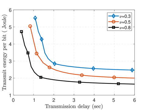
Figure 2: Energy and Delay trade-off for the $\mathit{PA}$ scheme

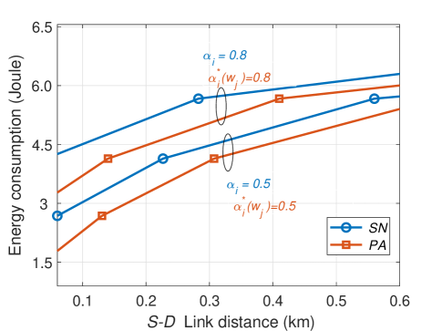
Figure 3: Energy consumption vs link distance for the $\mathit{PA}$ and $\mathit{SN}$ schemes

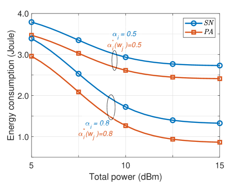
Figure 4: Energy consumption vs total power for the $\mathit{PA}$ and $\mathit{SN}$ schemes

Consider the following practical example to illustrate how the framework proposed can be implemented for UAV networks: transmitting signals, by Sa or Sb, over poor channel conditions consumes more energy than broadcasting over normal channel conditions. Under such a scenario, using the proposed method enables a user’s node to determine whether to send packets or leave the users idle based on the energy consumption. Then, the proposed approach ensures that energy consumption is conserved in UAV networks by creating a decision-making scheme. In order to clarify the characteristic of this decision-making platform, Fig. 3 illustrates the energy consumption curves versus total distance $d$, which represents the sum of $d_{a}$ and $d_{b}$. It is clearly shown that $\mathit{d}$ has a significant impact on energy consumption output as it decreases significantly with increasing $\mathit{d}$. This is because increasing $d_{a}$ requires a higher transmit power by $\mathit{S_{a}}$ node to suppress channel-fading growth, and, hence, higher energy consumption. This result agrees with what is observed in [47]. In addition, Fig. 3 shows that the proposed scheme allows energy consumption to be decreased by about 15% more than the $\mathit{SA}$ scheme.

Fig. 4 depicts that with the rise in power, $\mathcal{E}$ initially decreases and then reaches a constant. This is because $\mathcal{R}$ only increases logarithmically with $\mathrm{\mathit{\overline{P}}}$ while the transmission power consumption increases linearly with the transmission power [48]. Consequently, increasing power divides energy consumption into two stages. In the first stage, the energy is decreased; then, in the second stages, it approaches a constant rate. This reveals that there is a transition point that allows for the improvement of energy consumption. Fig. 4, illustrates that the domain of the transition point is between 13 and 17 dBm; and a further reduction of energy consumption is shown by the proposed method of $\mathit{PA,}$ which corresponds to previous studies [48, 49]. Further validation is given by Fig. 5, which compares the average data rate and the maximum transmit power. It is clear that the average data rate in (48) tends to become a constant at the high range of the transmit power (range between 14 and 16 dBm). This is because the power allocation strategy enables the transmit power to be regulated [50]. By using the $\mathit{PA}$ scheme, a higher average system rate is achieved, as the $\mathit{PA}$ minimises both $\mathcal{E}$ and $\mathit{q}$ (i.e., increases $\mathcal{R}$) simultaneously. Therefore, $\mathcal{R}$ increases logarithmically, while the transmission power consumption increases linearly with the transmission power [48]. In other words, the transition point is improved significantly, and such enhancement is expected to enhance other performance parameters in UAV networks. For example, Fig. 6 illustrates the relationship between distance and achievable data rate. It shows that increasing distance between $\mathit{S_{a}}$ and $\mathit{\mathit{S_{b}}}$ nodes gradually reduces achievable data rates due to high channel gain degradation. However, the $\mathit{PA}$ is always better than the $\mathit{SN}$, which agrees with other results obtained by [29].

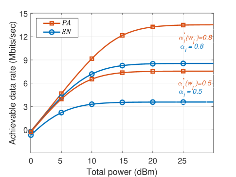
Figure 5: Achievable data rate vs total power for the $\mathit{PA}$ and $\mathit{SN}$ schemes

In the $\mathit{PA}$, the rate of distance change depends on flight altitude, and this is required to explain the effect of the drone altitude on data rate performance, as illustrated in Fig. 7. As depicted in the figure, when the drone takes off from the $\mathit{S_{a}}$ node level at 100 m, the data rate decreases slightly with the distance travelled by the drone remains within a low path loss range [51]. By increasing the altitude between $\mathit{S_{a}}$ node and drone, the path loss increases significantly and the data rate, in turn, starts to decrease gradually. The results of the proposed algorithm in the $\mathit{PA}$ show a marked improvement because increasing the altitude extend $d_{a}$ and, then, the arrival data rate at the relay is decreased. Hence, in addition to reducing transmission delay, both user nodes allocation of a higher power to each other in order to motivate information growth. The data rate curve is enhanced compared with other studies that depend on energy allocation only, as in [52]. To explain how the proposed $\overset{*}{\alpha_{i}}(w_{j})$ is allocated for the UAV network, Fig. 8 plots the relationship between $\overset{*}{\alpha_{i}}(w_{j})$ and both $\overline{P}$ and $w_{j}.$ It can be seen that increasing $\overline{P}$ allows $\overset{*}{\alpha_{i}}(w_{j})$ to be increased while notably decreasing $w_{j}$. The user nodes manage such a high $\overline{P}$ based on many factors, such as channel conditions or distance $d_{a}$ and $d_{b}$. Thus, if $d_{a}$ is higher than $d_{b},$ the path loss of $d_{a}$ is large and the rate at which data arrives at the relay is low. Therefore, the user nodes allocate higher $\overset{*}{\alpha_{i}}(w_{j})$ to stimulate an increase in data transmission by each user when there is an increase in delay time.

To evaluate UAV performance in (57), Fig. 9. shows results of $\text{\texthtb}_{e}[n]$ versus $\varphi_{i}$, and for various SNRs values, where $\overset{*}{\gamma}(w_{j})[n_{3}]>\overset{*}{\gamma}(w_{j})[n_{2}]>\overset{*}{\gamma}(w_{j})[n_{1}].$ Each $\overset{*}{\gamma}(w_{j})[n]$ is obtained from a specific value of $\varphi_{i}$ ($0<\varphi_{i}<1).$ It is clearly seen that the highest SNR, at $\overset{*}{\gamma}(w_{j})[n_{3}]$, enhanced the bit error rate result, and this result confirms the theoretical analysis, as high SNR calculates from optimal power allocation. This result agrees with previous studies [53], which indicate that the power allocation $\varphi_{i}$ is an effective metric for enhancing UAV performance.

Fig. 9. compares between the $SN$ and $PA$ system in term of $\varphi_{i}$ and bit error rate. Using energy allocation in (49) rises SNR[$\mathit{n}$] which in turn increases data rate, and the result enhancing bit error rate. Fig. 10. also shows that the highest SNR, i.e. $\textit{{SNR}}[n_{3}]>\textit{{SNR}}[n_{2}]>\textit{{SNR}}[n_{1}]$ $\textit{{SNR}}[n]\in\left\{\gamma(w_{j})[n],\overset{*}{\gamma}(w_{j})[n]\right\},$ gives the lower bit error rate. This result is consistent with previous results [54] for terrestrial communication systems. Obviously, a higher SNR results in better performance for the $PA$ as compare in $\mathit{SN}$, consequently, the proposed $\overset{*}{\text{\texthtb}}[n]$ can improve UAV performance.

Figure 6: Achievable data rate vs link distance for the $\mathit{PA}$ and $\mathit{SN}$ schemes

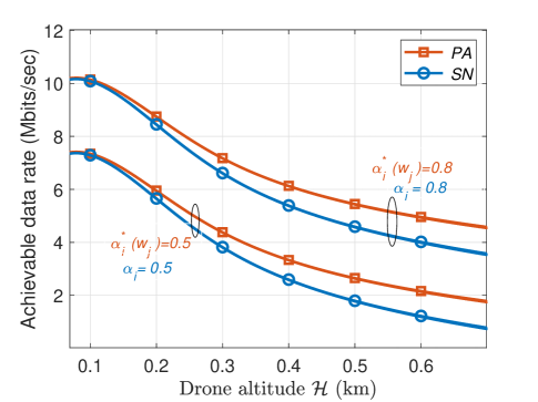
Figure 7: Achievable data rate vs altitude flight for the $\mathit{PA}$ and $\mathit{SN}$ schemes

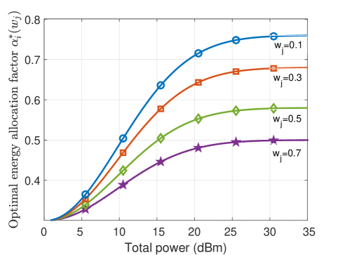
Figure 8: Achievable data rate vs total power for the $\mathit{PA}$ scheme

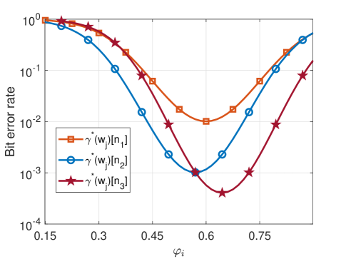
Figure 9: Power allocation vs bit error rate for the $\mathit{PA}$ scheme

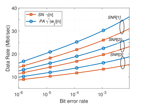
Figure 10: Achievable data rate vs bit error rate for the $\mathit{PA}$ and $\mathit{SN}$ schemes

VII Conclusion and Future Work

This paper offers a new method for drawing out the most effective energy-delay curve for a UAV layout by optimising the energy allotments for users and relay nodes. A multi-objective technique for optimising the energy allocation factors, weight scalarization optimisation, is appraised in this paper. The signal transmission distance is taken into consideration to evaluate UAVs. Simulations confirm the results originating from analytical expressions, and a real-world application scenario demonstrates how the proposed structure will be used. The paper concludes that the proposed technique effectively executes optimal decision-making and presents a compromise between energy and delay in UAVs. It would be interesting to extend our proposed study by considering future works’ weighted interval scheduling problem. Also, different system scenarios such as multiple UAVs could be employed instead of a single UAV. Besides that, statistical channel state information estimation can be used instead of instantaneous channel state information. Further, computational complexity is another direction that would be required to evaluate in future studies.

References

• [1] M. I. Khalil, “Energy efficiency maximization of relay aerial robotic networks,” IEEE Transactions on Green Communications and Networking, vol. 4, no. 4, pp. 1081–1090, 2020.
• [2] F. Ono, H. Ochiai, and R. Miura, “A wireless relay network based on unmanned aircraft system with rate optimization,” IEEE Transactions on Wireless Communications, vol. 15, no. 11, pp. 7699–7708, Nov 2016.
• [3] W. Zeng, J. Zhang, D. W. K. Ng, B. Ai, and Z. Zhong, “Two-way hybrid terrestrial-satellite relaying systems: Performance analysis and relay selection,” IEEE Transactions on Vehicular Technology, vol. 68, no. 7, pp. 7011–7023, 2019.
• [4] R. Zhang and J. Gorce, “Optimal transmission range for minimum energy consumption in wireless sensor networks,” in 2008 IEEE Wireless Communications and Networking Conference, 2008, pp. 757–762.
• [5] B. Zhou, L. Jiang, S. Zhao, and C. He, “BER analysis of TDD downlink multiuser MIMO systems with imperfect channel state information,” EURASIP Journal on Applied Signal Processing, vol. 2011, no. 1, Dec. 2011.
• [6] A. Zappone, L. Sanguinetti, and M. Debbah, “Energy-delay efficient power control in wireless networks,” IEEE Transactions on Communications, vol. 66, no. 1, pp. 418–431, 2018.
• [7] A. Brandt, Optimization Methods for Material Design of Cement-based Composites, ser. Modern Concrete Technology.   Taylor & Francis, 1998. [Online]. Available: https://books.google.com.au/books?id=RZTPi0V1JKEC
• [8] P. Nuggehalli, V. Srinivasan, and R. R. Rao, “Delay constrained energy efficient transmission strategies for wireless devices,” in Proceedings.Twenty-First Annual Joint Conference of the IEEE Computer and Communications Societies, vol. 3, 2002, pp. 1765–1772 vol.3.
• [9] Xiliang Zhong and Cheng-Zhong Xu, “Delay-constrained energy-efficient wireless packet scheduling with qos guarantees,” in GLOBECOM ’05. IEEE Global Telecommunications Conference, 2005., vol. 6, 2005, pp. 5 pp.–3340.
• [10] E. Uysal-Biyikoglu, B. Prabhakar, and A. El Gamal, “Energy-efficient packet transmission over a wireless link,” IEEE/ACM Transactions on Networking, vol. 10, no. 4, pp. 487–499, 2002.
• [11] M. A. Zafer and E. Modiano, “A calculus approach to minimum energy transmission policies with quality of service guarantees,” in Proceedings IEEE 24th Annual Joint Conference of the IEEE Computer and Communications Societies., vol. 1, 2005, pp. 548–559 vol. 1.
• [12] C. E. Shannon, “Probability of error for optimal codes in a gaussian channel,” The Bell System Technical Journal, vol. 38, no. 3, pp. 611–656, 1959.
• [13] Y. Polyanskiy, H. V. Poor, and S. Verdu, “Channel coding rate in the finite blocklength regime,” IEEE Transactions on Information Theory, vol. 56, no. 5, pp. 2307–2359, 2010.
• [14] ——, “Minimum energy to send $k$ bits through the gaussian channel with and without feedback,” IEEE Transactions on Information Theory, vol. 57, no. 8, pp. 4880–4902, 2011.
• [15] R. A. Berry and R. G. Gallager, “Communication over fading channels with delay constraints,” IEEE Transactions on Information Theory, vol. 48, no. 5, pp. 1135–1149, 2002.
• [16] O. Waqar, M. Imran, M. Dianati, and R. Tafazolli, “Energy consumption analysis and optimization of ber-constrained amplify-and-forward relay networks,” Vehicular Technology, IEEE Transactions on, vol. 63, no. 3, pp. 1256–1269, March 2014.
• [17] Y. Zeng, R. Zhang, and T. J. Lim, “Throughput maximization for uav-enabled mobile relaying systems,” IEEE Transactions on Communications, vol. 64, no. 12, pp. 4983–4996, Dec 2016.
• [18] Y. Chen, W. Feng, and G. Zheng, “Optimum placement of uav as relays,” IEEE Communications Letters, vol. 22, no. 2, pp. 248–251, Feb 2018.
• [19] X. Jiang, Z. Wu, Z. Yin, and Z. Yang, “Power and trajectory optimization for uav-enabled amplify-and-forward relay networks,” IEEE Access, vol. 6, pp. 48 688–48 696, 2018.
• [20] K. Govindan, K. Zeng, and P. Mohapatra, “Probability density of the received power in mobile networks,” IEEE Transactions on Wireless Communications, vol. 10, no. 11, pp. 3613–3619, 2011.
• [21] A. Al-Hourani, S. Kandeepan, and S. Lardner, “Optimal lap altitude for maximum coverage,” IEEE Wireless Communications Letters, vol. 3, no. 6, pp. 569–572, 2014.
• [22] M. Alzenad, A. El-Keyi, F. Lagum, and H. Yanikomeroglu, “3-d placement of an unmanned aerial vehicle base station (uav-bs) for energy-efficient maximal coverage,” IEEE Wireless Communications Letters, vol. 6, no. 4, pp. 434–437, 2017.
• [23] M. Mozaffari, W. Saad, M. Bennis, and M. Debbah, “Unmanned aerial vehicle with underlaid device-to-device communications: Performance and tradeoffs,” IEEE Transactions on Wireless Communications, vol. 15, no. 6, pp. 3949–3963, June 2016.
• [24] S. Zhang, H. Zhang, Q. He, K. Bian, and L. Song, “Joint trajectory and power optimization for uav relay networks,” IEEE Communications Letters, vol. 22, no. 1, pp. 161–164, 2018.
• [25] M. Mozaffari, W. Saad, M. Bennis, and M. Debbah, “Mobile unmanned aerial vehicles (uavs) for energy-efficient internet of things communications,” IEEE Transactions on Wireless Communications, vol. 16, no. 11, pp. 7574–7589, 2017.
• [26] M. Luo, G. Villemaud, J. M. Gorce, and J. Zhang, “Realistic prediction of ber and amc for indoor wireless transmissions,” IEEE Antennas and Wireless Propagation Letters, vol. 11, pp. 1084–1087, 2012.
• [27] M. I. Khalil, “Delay and energy balance for unmanned aerial vehicle networks,” in 2021 IEEE 11th Annual Computing and Communication Workshop and Conference (CCWC), 2021, pp. 1453–1458.
• [28] O. Weck, “Multiobjective optimization : History and promise,” in MULTIOBJECTIVE OPTIMIZATION : HISTORY AND PROMISE, 2004.
• [29] C. Tian, Z. Qian, X. Wang, and L. Hu, “Analysis of joint relay selection and resource allocation scheme for relay-aided d2d communication networks,” IEEE Access, vol. 7, pp. 142 715–142 725, 2019.
• [30] D. Yang, Q. Wu, Y. Zeng, and R. Zhang, “Energy tradeoff in ground-to-uav communication via trajectory design,” IEEE Transactions on Vehicular Technology, vol. 67, no. 7, pp. 6721–6726, July 2018.
• [31] Y. Li, X. Zhang, M. Peng, and W. Wang, “Power provisioning and relay positioning for two-way relay channel with analog network coding,” IEEE Signal Processing Letters, vol. 18, no. 9, pp. 517–520, Sept 2011.
• [32] M. Khalil, S. Berber, and K. Sowerby, “High snr approximation for performance analysis of two-way multiple relay networks,” Physical Communication, vol. 24, pp. 62 – 70, 2017. [Online]. Available: http://www.sciencedirect.com/science/article/pii/S1874490716301446
• [33] A. S. Y. Poon, D. N. C. Tse, and R. W. Brodersen, “An adaptive multiantenna transceiver for slowly flat fading channels,” IEEE Transactions on Communications, vol. 51, no. 11, pp. 1820–1827, 2003.
• [34] J. Zander, “Radio resource management in future wireless networks: requirements and limitations,” IEEE Communications Magazine, vol. 35, no. 8, pp. 30–36, 1997.
• [35] Y. Zhang, Y. Ma, and R. Tafazolli, “Power allocation for bidirectional af relaying over rayleigh fading channels,” Communications Letters, IEEE, vol. 14, no. 2, pp. 145–147, 2010, iD: 1.
• [36] A. B. Kiely and J. T. Coffey, “On the capacity of a cascade of channels,” IEEE Transactions on Information Theory, vol. 39, no. 4, pp. 1310–1321, 1993.
• [37] S. Salehkalaibar, M. Wigger, and L. Wang, “Hypothesis testing over cascade channels,” in 2017 IEEE Information Theory Workshop (ITW), 2017, pp. 369–373.
• [38] J. Ren, G. Yu, Y. He, and G. Y. Li, “Collaborative cloud and edge computing for latency minimization,” IEEE Transactions on Vehicular Technology, vol. 68, no. 5, pp. 5031–5044, 2019.
• [39] J. Koski, “Defectiveness of weighting method in multicriterion optimization of structures,” Communications in Applied Numerical Methods, vol. 1, no. 6, pp. 333–337, 1985. [Online]. Available: https://onlinelibrary.wiley.com/doi/abs/10.1002/cnm.1630010613
• [40] T. B. To and U. Korn, “An evolution strategy for the multiobjective optimization,” The Second International Conference on Genetic Algorithms, Brno, Czech Republic, 01 1996.
• [41] G. Farhadi and N. C. Beaulieu, “On the performance of amplify-and-forward cooperative systems with fixed gain relays,” Wireless Communications, IEEE Transactions on, vol. 7, no. 5, pp. 1851–1856, 2008.
• [42] M. Hasna and M.-S. Alouini, “Harmonic mean and end-to-end performance of transmission systems with relays,” Communications, IEEE Transactions on, vol. 52, no. 1, pp. 130–135, Jan 2004.
• [43] ——, “End-to-end performance of transmission systems with relays over rayleigh-fading channels,” Wireless Communications, IEEE Transactions on, vol. 2, no. 6, pp. 1126–1131, Nov 2003.
• [44] R. H. Louie, Y. Li, H. Suraweera, and B. Vucetic, “Performance analysis of beamforming in two hop amplify and forward relay networks with antenna correlation,” Wireless Communications, IEEE Transactions on, vol. 8, no. 6, pp. 3132–3141, June 2009.
• [45] Z. Wang and G. Giannakis, “A simple and general parameterization quantifying performance in fading channels,” Communications, IEEE Transactions on, vol. 51, no. 8, pp. 1389–1398, Aug 2003.
• [46] B. Gurakan, O. Ozel, and S. Ulukus, “Optimal energy and data routing in networks with energy cooperation,” IEEE Transactions on Wireless Communications, vol. 15, no. 2, pp. 857–870, 2016.
• [47] K. Yang, S. Martin, C. Xing, J. Wu, and R. Fan, “Energy-efficient power control for device-to-device communications,” IEEE Journal on Selected Areas in Communications, vol. 34, no. 12, pp. 3208–3220, 2016.
• [48] C. Xiong, G. Y. Li, S. Zhang, Y. Chen, and S. Xu, “Energy-efficient resource allocation in ofdma networks,” IEEE Transactions on Communications, vol. 60, no. 12, pp. 3767–3778, 2012.
• [49] D. W. K. Ng, E. S. Lo, and R. Schober, “Energy-efficient resource allocation in ofdma systems with large numbers of base station antennas,” IEEE Transactions on Wireless Communications, vol. 11, no. 9, pp. 3292–3304, 2012.
• [50] ——, “Energy-efficient resource allocation in multi-cell ofdma systems with limited backhaul capacity,” IEEE Transactions on Wireless Communications, vol. 11, no. 10, pp. 3618–3631, 2012.
• [51] W. Khawaja, I. Guvenc, D. W. Matolak, U. Fiebig, and N. Schneckenburger, “A survey of air-to-ground propagation channel modeling for unmanned aerial vehicles,” IEEE Communications Surveys Tutorials, vol. 21, no. 3, pp. 2361–2391, 2019.
• [52] L. Sboui, H. Ghazzai, Z. Rezki, and M. Alouini, “Achievable rates of uav-relayed cooperative cognitive radio mimo systems,” IEEE Access, vol. 5, pp. 5190–5204, 2017.
• [53] M. Mondelli, Q. Zhou, X. Ma, and V. Lottici, “A cooperative approach for amplify-and-forward differential transmitted reference ir-uwb relay systems,” in 2012 IEEE International Conference on Acoustics, Speech and Signal Processing (ICASSP), 2012, pp. 2905–2908.
• [54] W. Al-Hanafy and S. Weiss, “Discrete rate maximisation power allocation with enhanced bit error ratio,” IET Communications, vol. 6, pp. 1019–1024(5), June 2012.