Type-aware Embeddings for Multi-Hop Reasoning over Knowledge Graphs

Abstract

Multi-hop reasoning over real-life knowledge graphs (KGs) is a highly challenging problem as traditional subgraph matching methods are not capable to deal with noise and missing information. To address this problem, it has been recently introduced a promising approach based on jointly embedding logical queries and KGs into a low-dimensional space to identify answer entities. However, existing proposals ignore critical semantic knowledge inherently available in KGs, such as type information. To leverage type information, we propose a novel TypE-aware Message Passing (Temp) model, which enhances the entity and relation representations in queries, and simultaneously improves generalization, deductive and inductive reasoning. Remarkably, Temp is a plug-and-play model that can be easily incorporated into existing embedding-based models to improve their performance. Extensive experiments on three real-world datasets demonstrate Temp’s effectiveness.

1 Introduction

In recent years, the multi-hop reasoning problem of answering first-order logic queries (FOL) on large-scale incomplete knowledge graphs (KGs) Pan et al. (2016) has gained a lot of attention in the AI community. A major challenge for traditional subgraph matching methods for query answering is that KGs are inevitably incomplete and noisy. Indeed, when schema Wiharja et al. (2020) and triples are incomplete in the KG, correct answers are not guaranteed to be found under normal deductive reasoning, leading to empty or wrong answers. Another problem is their intrinsic high computational complexity as they need to keep track of all intermediate entities occurring on reasoning paths, leading to an exponential blow-up. For instance, to answer the query “List the presidents of Asian countries that have held the Summer Olympics” shown in Fig. 1, we require two traversing-steps (many more for other queries): one to identify countries that have held the summer Olympics and another one to identify Asian countries, each producing intermediate countries.

To address these challenges, a query embedding (QE) approach to query answering has been recently introduced as an alternative to subgraph matching methods. The main idea is to embed entities and queries into a joint low-dimensional vector space such that entities that answer the query are close to the embedding of the query. Several QE models for query answering, showing very promising performance, have been proposed so far Hamilton et al. (2018); Ren et al. (2020); Ren and Leskovec (2020); Zhang et al. (2021); Choudhary et al. (2021b); Luus et al. (2021). However, these models fail to leverage semantic knowledge inherently available in KGs, such as entity description Yao et al. (2019); Daza et al. (2021) or entity type information Niu et al. (2020); Pan et al. (2021). Advantages of introducing type information are that: 1) it can enhance the representation of entities or relations; e.g., the types sports and event can enrich the representation of the entity Summer Olympics in the context of sport events (cf.  Fig. 1). 2) It can also help tackling the inductive query answering problem where entities used in test queries cannot be observed at training time; e.g., consider the queries in Figure 1: “List the presidents of Asian countries that have held the Summer Olympics” and “List the presidents of European countries that have held the Winter Olympics”, which are generated from two KGs with disjoint sets of entities: Train KG and Test KG, respectively. Even if the entities Summer Olympics and Winter Olympics are different, they have similar type information, such as sports and event. Consequently, after using type information to represent entities, the model associated to the query generated from Train KG is also effective on the query generated from Test KG.

The goal of this paper is to introduce a type-aware plug-and-play model which makes full use of type information in the knowledge graph, and can be easily embedded into existing QE-based models. To this aim, we propose a novel TypE-aware Message Passing (Temp) model, which contains two key components. 1) Type-aware Entity Representations (TER), aggregating type information of entities to strengthen their vector representation (cf. Section 4.1). 2) Type-aware Relation Representations (TRR), using entity type information to construct a global type graph to enhance the relation representation, and simultaneously integrate it with its type representation and existing entity type information (cf. Section 4.2). Importantly, some queries have variable nodes in the query paths (see Figure 1), which increase the difficulty of subsequent reasoning steps in the chain, as variable nodes are unknown. To address this, the TRR component uses a bidirectional mechanism for the anchor node to supervise the relations in the query path, and vice versa. Furthermore, as mentioned, after using type information to represent entities and relations, the model becomes inherently inductive as the occurrence of new entities or relations will not affect the type-based representations.

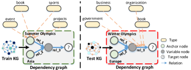
Figure 1: Inductive setting for FOL queries. The left part shows the query “List the presidents of Asian countries that have held the Summer Olympics”. The right part shows the query “List the presidents of European countries that have held the Winter Olympics”. rel_1, rel_2, and rel_3 represent relations: Hold, Locate, and President of, respectively.

Our main contributions can be summarized as follows:

• We propose Temp, a novel type-aware plug-and-play model for multi-hop reasoning over KGs, that can be easily incorporated into the existing QE-based models.

• We design a new bidirectional integration mechanism that incorporates the pairwise dependencies among {entity, relation, type} information, even in the absence of schema axioms like domain and range.

• Extensive experiments demonstrate that after incorporating Temp into four state-of-the-art baselines, their generalization, deductive and inductive reasoning abilities are significantly improved across three benchmark datasets consistently.

Data, code, and an extended version with appendix is available at https://github.com/zhiweihu1103/QE-TEMP

2 Related Work

Query Embeddings.

QE models first embed entities and FOL queries into a joint low-dimensional vector space, and subsequently compute a similarity score between the entity representation and query representation in the latent embedding space. In general, according to the type of embedding spaces, QE-based methods can be divided into four categories: (i) geometric-based methods, such as GQE Hamilton et al. (2018), Q2B Ren et al. (2020), HypE Choudhary et al. (2021b), and ConE Zhang et al. (2021), where logical queries and KG entities are embedded into a geometric vector space as points, boxes, hyperbolic, and cone shapes, respectively; (ii) distribution-based methods, such as BetaE Ren and Leskovec (2020), embedding queries to beta distributions with bounded support, and PERM Choudhary et al. (2021a), using Gaussian densities to reason over KGs; (iii) logic-based methods, relating so-called set logic with FOL  Luus et al. (2021); (iv) neural-based methods, e.g., EMQL Sun et al. (2020) using neural retrieval to implement logical operations. Considering QE-based methods are the mainstream in the current CQA field, we mainly focus on how to construct a plug-and-play model to embed the type information for existing QE-based methods.

Other Methods.

Besides the QE-based approach, the path-based approach is another method for CQA, but it faces an exponential growth of the search space with the number of hops. For instance, CQD Arakelyan et al. (2021) uses a beam search method to explicitly track intermediate entities, and repeatedly combines scores from a pretrained link predictor via t-norms to search answers while tracking intermediaries. However, CQD does not support the full set of FOL queries.

Inductive KG Completion (KGC).

In the context of KGC, there have been some works on inductive settings where test entities are not seen in the training stage. Based on the source of information used, they can be split into two categories: Using graph structure information, e.g., subgraph or topology structures Teru et al. (2020); Chen et al. (2021); Wang et al. (2021), or using external information, e.g., textual descriptions of entities Daza et al. (2021). However, all these methods focus on the inductive KGC task, which can be seen as answering simpler one-hop queries.

Type-aware Tasks.

Type information was previously used in other tasks such as KGC or entity typing Yao et al. (2019); Zhao et al. (2020); Daza et al. (2021); Niu et al. (2020); Pan et al. (2021). However, these works cannot be directly used for answering FOL queries because this requires multi-hop reasoning, producing intermediate uncertain entities.

3 Background

In this paper, a knowledge graph Pan et al. (2016) is represented in a standard format for graph-structured data such as RDF. A knowledge graph $\mathcal{G}$ is a tuple $(\mathcal{E},\mathcal{R},\mathcal{C},\mathcal{T})$, where $\mathcal{E}$ is a set of entities, $\mathcal{R}$ is a set of relation types, $\mathcal{C}$ is a set of entity types, and $\mathcal{T}$ is a set of triples. Triples in $\mathcal{T}$ are either relation assertions $(h,r,t)$, where $h,t\in\mathcal{E}$ are respectively the head and tail entities of the triple, and $r\in\mathcal{R}$ is the edge of the triple connecting head and tail, or entity type assertions ($e$, $type$, $c$), where $e\in\mathcal{E}$ is an entity, $c\in\mathcal{C}$ is an entity type and $type$ is the instance-of relation Pan (2009).

We consider FOL queries that use existential quantification ($\exists$), conjunction ($\wedge$), disjunction ($\vee$) and negation ($\neg$) operations. We will work with FOL queries in Disjunctive Normal Form, i.e. represented as a disjunction of conjunctions. To introduce FOL queries, we assume that $\mathcal{V}_{a}\subset\mathcal{E}$ represents a set of non-variable input anchor entities, $V_{1},\ldots,V_{m}$ denote existentially quantified variables and $V_{?}$ is the target variable. A FOL query $\mathcal{Q}$ is a formula of the following form:

$$\mathcal{Q}[V_{?}]= \,\,V_{?}\,.\,\exists V_{1},\ldots,V_{m}:c_{1}\vee c_{2}\vee\ldots\vee c_{n}$$

where $c_{i}=e_{i1}\wedge\ldots\wedge$ $e_{ik}$, k $\leq$ m such that each $e_{ij}$ is of one of the following forms: $r(V_{a},V)$, $\neg r(V_{a},V)$, $r(V_{,}V^{\prime})$ or $\neg r(V,V^{\prime})$, with $V_{a}\in\mathcal{V}_{a}$, $V\in\{V_{?},V_{1},\ldots,V_{m}\}$, $V^{\prime}\in\{V_{1},\ldots,V_{m}\}$, $V\neq V^{\prime}.$

The dependency graph (DG) of a query $\mathcal{Q}$ is a graphical representation of $\mathcal{Q}$, where nodes correspond to variable or non-variable arguments in $\mathcal{Q}$ and edges correspond to relations in $\mathcal{Q}$. Figure 1 shows an example of a DG.

We are interested in the multi-hop reasoning problem of answering queries $\mathcal{Q}$ on KGs, which aims to find a set of entities $\llbracket\mathcal{Q}\rrbracket\subseteq\mathcal{E}$ such that $a\in\llbracket\mathcal{Q}\rrbracket$ iff $\mathcal{Q}[a]$ holds true.

4 Semantically-enriched Embeddings

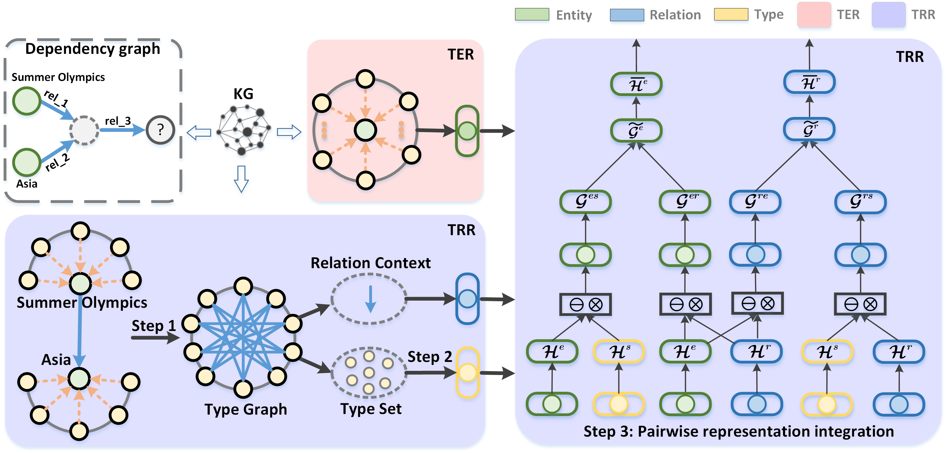
Figure 2: Temp’s Architecture. The left top part is the dependency graph for query “List the presidents of Asian countries that have held the Summer Olympics”, rel_1, rel_2, and rel_3 represent the relations Hold, Locate, and President of, respectively.

Our model Temp is composed of two sub-models: Type-aware Entity Representations (TER), which uses type information of an entity to enrich its vector representation, and Type-aware Relation Representations (TRR), which further integrates entity representations, relation types, and relation representations to strengthen the entity and relation vector representations simultaneously. Interestingly, as we only leverage type information to perform an in-depth characterization of entities and relations without modifying the training target of existing QE-based models, Temp can be easily embedded into them in a plug-and-play fashion.

4.1 TER: Type-aware Entity Representations

The main intuition behind TER is that the types of an entity provide valuable information about what it represents in the KG. For instance, if an entity contains types such as sports/multi_event_tournament, time/event, olympics/olympic_games, it is plausible to infer that the corresponding entity represents Olympics. To capture this intuition, we design an iterative multi-highway layer Srivastava et al. (2015) to aggregate the type information in entity type assertions to get a more accurate and comprehensive representation of it. Let $\mathcal{H}_{s}^{i}\in\mathbb{R}^{d\times n}$ denote the hidden state of type information of an entity in iteration $i\geq 1$, where d and n respectively represent the vector size and the number of types of an entity. The highway-based type fusion representation of a given entity can be calculated as follows:

$$g=\sigma(W_{i}\mathcal{H}_{s}^{i}+b_{i})$$ (1)

$$\mathcal{H}_{s}^{i+1}=g\ast(W_{i}^{\prime}\mathcal{H}_{s}^{i}+b_{i}^{\prime})+(1-g)\ast\mathcal{H}_{s}^{i}$$ (2)

$$\widetilde{\mathcal{H}_{s}^{K}}=W\mathcal{H}_{s}^{K}+b$$ (3)

$\mathcal{H}_{s}^{1}$ is the initial feature of types of an entity, $\sigma$ is an element-wise sigmoid function, {$W_{i},W_{i}^{\prime}$}$\in\mathbb{R}^{d\times d}$, {$b_{i},b_{i}^{\prime}$}$\in\mathbb{R}^{d\times 1}$ are learnable matrices, and g$\in\mathbb{R}^{d\times n}$ is the reset gate. After iterating K times (we set K=2), the final message $\mathcal{H}_{s}^{K}\in\mathbb{R}^{d\times n}$ (undergoing a linear operation to obtain $\widetilde{\mathcal{H}_{s}^{K}}\in\mathbb{R}^{d\times 1}$) is taken as the representation for the types of a given entity. We further concatenate the initial entity and its type aggregation representation to get an enhanced entity representation.

$$\mathcal{H}^{e}=W^{\prime}[\widetilde{\mathcal{H}_{s}^{K}},\mathcal{H}_{s}^{0}]+b^{\prime},$$ (4)

where [$\cdot$] is the concatenation function, $W^{{}^{\prime}}$$\in\mathbb{R}^{d\times d}$ and $b^{{}^{\prime}}$$\in\mathbb{R}^{d\times 1}$ are the parameters to learn. $\mathcal{H}^{e}\in\mathbb{R}^{d\times 1}$ is the final representation of the entity. It is important to note that for inductive reasoning, we will not concatenate with the initial entity information $\mathcal{H}_{s}^{0}$ as the entities seen during training are not presented in the test phase. The process is shown in top center of Figure 2.

4.2 TRR: Type-aware Relation Representations

Performing TER on entities is useful for queries without existentially quantified variables. However, for queries with chained existential variables (chain of variable nodes in the DG) it is not enough to only perform TER on the anchor entity or target variable. Intuitively, the problem is that in the long-chain reasoning process, the correlation between the anchor entity and target variable may not be strong enough after several relation projections. Besides, continuous relational projections may cause exponential growth in the search space, further increasing the complexity of the model.

We start by observing that the types of a relation are correlated with its representation in the KG. For example, assuming a relation $r$ has types government/ political_appointer and organization/role, then we can plausibly infer that the relation $r$ represents President of. In long-chain queries, type-enhancement on relations can help to reduce the answer entity space and cascading errors caused by multiple projections. However, in most existing KGs, relations lack specific type annotations (such as domain and range). We address this problem by building, based on the original KG, a novel type graph with types as nodes and relations as edges (see bottom left of Fig. 2). In a subsequent step, we aggregate the type information on the type graph to obtain the type embedding corresponding to a specific relation. Finally, we integrate the entity representation, the aggregated type information of a relation and its representation by a bidirectional attention mechanism, so that the intermediate variable nodes can perceive the message of anchor or target nodes and of the relations in the chain of reasoning (see right of Fig. 2). This will help to avoid the weakening of the connection between anchor and target entity caused by long-chain reasoning.

4.2.1 Step 1: Type Graph Construction

We formally define a type graph $\mathcal{G}_{\mathsf{tp}}$. Let $\mathcal{G}=(\mathcal{E,R,C,T})$ be a KG. For a relation $r\in\mathcal{R}$, $\mathcal{T}_{r}\subseteq\mathcal{T}$ denotes the set of relation assertions in which $r$ occurs. For a relation assertion $\mathsf{t}\in\bigcup_{r\in\mathcal{R}}\mathcal{T}_{r}$, $\mathsf{hd}(\mathsf{t})$ and $\mathsf{tl}(\mathsf{t})$ respectively denote the head and tail entities of $\mathsf{t}$, and $\mathsf{tp}_{\mathsf{t}}(\mathsf{hd}(\mathsf{t}))=\{c\mid(\mathsf{hd}(\mathsf{t}),type,c)\in\mathcal{T}\}$ denotes the set of types of the head of $\mathsf{t}$; $\mathsf{tp}_{\mathsf{t}}(\mathsf{tl}(\mathsf{t}))$ is defined analogously. Since $r$ may occur in multiple relation assertions, we will compute the type information of $r$ by taking the intersection of the types of the head and tail entities of relation assertions in which $r$ occurs. For $r\in\mathcal{R}$, we define

$$\mathsf{tp}_{r}^{\mathsf{hd}}(\mathcal{G})=\bigcap_{\mathsf{t}\in\mathcal{T}_{r}}\mathsf{tp}_{\mathsf{t}}(\mathsf{hd}(\mathsf{t})),\qquad\mathsf{tp}_{r}^{\mathsf{tl}}(\mathcal{G})=\bigcap_{\mathsf{t}\in\mathcal{T}_{r}}\mathsf{tp}_{\mathsf{t}}(\mathsf{tl(t)}).\vspace{-0.1cm}$$

In addition, we define $\mathcal{G}_{\mathsf{tp}}=(V,E,T)$ by setting $V=\bigcup_{r\in\mathcal{R}}\mathsf{tp}^{\mathsf{hd}}_{r}(\mathcal{G})\cup\mathsf{tp}^{\mathsf{tl}}_{r}(\mathcal{G})$ , $E=\mathcal{R}$, and $(v,r,v^{\prime})\in T$ if there exists $\mathsf{t}\in\mathcal{T}_{r}$ such that $v=\mathsf{tp}_{\mathsf{t}}(\mathsf{hd(t)})$ and $v^{\prime}=\mathsf{tp}_{\mathsf{t}}(\mathsf{tl(t)})$.

4.2.2 Step 2: Relation Type Aggregation

For a given relation $r\in E$, we define the types associated with a relation as $\mathsf{tp}_{r}(\mathcal{G}_{\mathsf{tp}})$ = $\mathsf{tp}^{\mathsf{hd}}_{r}(\mathcal{G})\cup\mathsf{tp}^{\mathsf{tl}}_{r}(\mathcal{G})$. We fix an arbitrary linear order on the elements of $\mathsf{tp}_{r}(\mathcal{G}_{\mathsf{tp}})$, and denote by $\mathsf{tp}^{i}_{r}(\mathcal{G}_{\mathsf{tp}})$ the $i$-th type, for all $1\leq i\leq|\mathsf{tp}_{r}(\mathcal{G}_{\mathsf{tp}})|$. Note that not all types in $\mathsf{tp}_{r}(\mathcal{G}_{\mathsf{tp}})$ are relevant for answering a given query. For example, assume that the relation has_part contains the types {vehicle, animal, universe}. For the query “What organs are parts of a cat?”, we should give type animal more attention, but for the query “What components are parts of a car?” we should concentrate on the type vehicle. So, instead of simply concatenating (or averaging) all the type information associated to a relation, we model the relation type aggregation as an attention neural network, defined as:

$$\mathcal{H}^{s}=\sum_{i}a_{i}\odot\mathcal{H}_{s}^{i}$$ (5)

$$a_{i}=\frac{exp(\textbf{MLP}(\mathcal{H}_{r}^{i}))}{\sum_{j}exp(\textbf{MLP}(\mathcal{H}_{r}^{j}))}$$ (6)

$\mathcal{H}^{s}$ is the vector representation of the aggregated type information $\mathsf{tp}_{r}(\mathcal{G}_{\mathsf{tp}})$; $\mathcal{H}_{s}^{i}\in{\mathbb{R}^{d\times 1}}$ is the vector representation of the i-th type $\mathsf{tp}_{r}^{i}(\mathcal{G}_{\mathsf{tp}})$, which is initialized to a uniform distribution with dimension d, $1\leq i\leq|\mathsf{tp}_{r}^{i}(\mathcal{G}_{\mathsf{tp}})|$; $a_{i}\in{\mathbb{R}^{d\times 1}}$ is a positive weight vector that satisfies $\sum_{i=1}^{n}[a_{i}]_{j}=1$ for all $1\leq j\leq d$; and MLP($\cdot$) : $\mathbb{R}^{d}\rightarrow\mathbb{R}^{d}$ is a multi-layer perceptron network.

4.2.3 Step 3: Pairwise Representation Integration

When embedding queries, integrating the information of entities, relations, and types can help to smooth decision boundaries, but this needs to be done in a way that the intended match of the query into the KG is captured. For example, for the query “Which countries have held the Summer Olympics?”, we need to concentrate on Held connections from Summer Olympics, rather than e.g., Watch connections. Analogously, we should only consider Held connections starting at Summer Olympics, rather than e.g., at World Cup. To properly capture this restriction in the triple {$\mathcal{H}^{e}$, $\mathcal{H}^{r}$, $\mathcal{H}^{s}$} ($\mathcal{H}^{e}$ and $\mathcal{H}^{s}$ defined as in Equations (4) and (5), and $\mathcal{H}^{r}$ is the initialization relation vector), we introduce a bidirectional attention mechanism Zhang et al. (2020) to integrate each state of pairwise representation pairs: entity-relation, entity-type, and relation-type. Here, we show how to do this for entity-relation pair. Bidirectional integration representation between $\mathcal{H}^{e}$ and $\mathcal{H}^{r}$ can be calculated as follows:

$$\mathcal{G}^{er}=Relu(W_{1}\begin{bmatrix}\mathcal{H}^{e}\ominus\mathcal{H}^{r}\\ \mathcal{H}^{e}\otimes\mathcal{H}^{r}\end{bmatrix}+b_{1})$$ (7)

$$\mathcal{G}^{re}=Relu(W_{2}\begin{bmatrix}\mathcal{H}^{r}\ominus\mathcal{H}^{e}\\ \mathcal{H}^{r}\otimes\mathcal{H}^{e}\end{bmatrix}+b_{2})$$ (8)

$\{W_{1},W_{2}\}\in\mathbb{R}^{2d\times 2d}$ and {$b_{1},b_{2}\}\in\mathbb{R}^{2d\times 1}$ are learnable parameters. We use element-wise subtraction $\ominus$ and multiplication $\otimes$ to build better matching representations Tai et al. (2015). $\mathcal{G}^{er}\in\mathbb{R}^{2d\times 1}$ is the result of integrating entity relation information. Through bidirectional integration of entities and relations, we simultaneously get a relation-aware entity representation and an entity-aware relation representation, capturing the interaction between entities and relations.

We then use a gated mechanism to combine the results produced by bidirectional fusion as it better regulates the information flow Srivastava et al. (2015). Take the entity fusion representation as an example, using the relation-aware entity $\mathcal{G}^{er}$ and type-aware entity $\mathcal{G}^{es}$ representations as input, the final representation of entity is computed as

$$g=\sigma(W_{3}\mathcal{G}^{er}+W_{4}\mathcal{G}^{es}+b_{3}+b_{4})$$ (9)

$$\widetilde{\mathcal{G}^{e}}=g\ast\mathcal{G}^{er}+(1-g)\ast\mathcal{G}^{es}$$ (10)

{$W_{3}$, $W_{4}$} $\in$ $\mathbb{R}^{2d\times 2d}$ and {$b_{3}$, $b_{4}$} $\in$ $\mathbb{R}^{2d\times 1}$ are the parameters to learn. g is the reset gate, and $\widetilde{\mathcal{G}^{e}}\in\mathbb{R}^{2d\times 1}$ is the final entity representation.

To transform the fused feature to the original vector size, we use one linear layer: $\overline{\mathcal{H}^{e}}=W_{5}\widetilde{\mathcal{G}^{e}}+b_{5}$, where $W_{5}$ $\in$ $\mathbb{R}^{d\times 2d}$ and $b_{5}$ $\in$ $\mathbb{R}^{d\times 1}$ are learnable parameters. $\overline{\mathcal{H}^{e}}$ is the final entity representation enhanced by relation and type.

5 Experiments

(a) Generalization on FB15k-237 (Q2B datasets)											FB15k	NELL
Method	1p	2p	3p	2i	3i	pi	ip	2u	up	Avg	Avg	Avg
GQE	41.3	21.5	15.2	26.5	38.5	16.7	8.8	17.1	15.8	22.4	40.1	23.5
+Temp	47.6	29.6	24.7	36.3	48.4	25.5	13.4	30.2	21.0	30.7	56.6	38.2
Q2B	47.1	24.9	19.4	33.2	46.4	21.8	11.3	25.3	19.3	27.6	51.2	31.1
+Temp	45.7	27.8	23.4	36.9	49.6	22.9	11.7	27.6	18.9	29.4	55.4	37.3
BetaE	42.6	25.4	21.6	30.2	43.3	20.7	9.2	24.2	18.3	26.2	50.6	33.4
+Temp	43.3	27.2	22.7	35.3	47.5	24.3	10.6	26.7	18.2	28.4	53.6	34.5
LogicE	45.6	27.8	24.1	34.7	46.5	23.5	12.0	27.1	20.8	29.1	54.2	39.1
+Temp	46.6	29.2	25.0	35.8	47.9	24.9	13.5	28.7	21.0	30.3	55.7	39.1
(b) Deductive Reasoning on FB15k-237 (Q2B datasets)											FB15k	NELL
GQE	56.4	30.1	24.5	35.9	51.2	25.1	13.0	25.8	22.0	31.6	43.7	49.8
+Temp	76.3	48.6	39.0	49.7	60.4	36.9	22.1	59.0	36.3	47.6	71.4	75.5
Q2B	58.5	34.3	28.1	44.7	62.1	23.9	11.7	40.5	22.0	36.2	43.7	51.1
+Temp	87.2	59.6	47.9	67.2	72.7	49.1	29.8	78.6	43.4	59.5	69.6	90.4
BetaE	77.9	52.6	44.5	59.0	67.8	42.2	23.5	63.7	35.1	51.8	60.6	80.2
+Temp	84.7	58.3	49.4	62.3	68.8	45.3	28.5	74.5	41.1	57.0	60.6	81.5
LogicE	81.5	54.2	46.0	58.1	67.1	44.0	28.5	66.6	40.8	54.1	65.5	85.3
+Temp	84.5	59.8	51.9	59.3	68.1	47.0	33.4	70.8	45.4	57.8	67.1	84.6

Table 1: Hits@3 results on the Q2B datasets testing generalization and deductive reasoning. Please see appendix for full results on FB15k and NELL.

Our aim is to analyse the impact of adding Temp to existing QE models on their generalization, deductive and inductive reasoning abilities.

Datasets and Queries.

For generalization and deductive reasoning, we use three standard benchmark KGs with official training/validation/test splits: FB15k Bordes et al. (2013), FB15k-237 Toutanova and Chen (2015), and NELL995 (NELL) Xiong et al. (2017), and two query datasets: one with 9 query structures without negation from Query2Box (Q2B) Ren et al. (2020) and another with 14 (9 positive + 5 with negation) from BetaE Ren and Leskovec (2020). To test inductive reasoning, we use the datasets FB15k-237-V2 and NELL-V3 provided by GraIL Teru et al. (2020), ensuring that the test and training sets have a disjoint set of entities. Note that we generate queries over these datasets as done for BetaE datasets. We choose Hit@K and Mean Reciprocal Rank (MRR) as two evaluation metrics.

Baselines.

We embed Temp on four state-of-the-art baselines for complex QA on KGs: Q2B, BetaE, GQE Hamilton et al. (2018), and LogicE Luus et al. (2021).

Generalization.

The goal is to find non-trivial answers to FOL queries over incomplete KGs, i.e. answers cannot get using subgraph matching. We follow the evaluation protocol in Ren and Leskovec (2020). Briefly, three KGs are built: $\mathcal{G}_{\textit{train}}$ containing only training triples, $\mathcal{G}_{\textit{valid}}$ containing $\mathcal{G}_{\textit{train}}$ plus validation triples, and $\mathcal{G}_{\textit{test}}$ containing $\mathcal{G}_{\textit{valid}}$ as well as test triples. The models are trained using $\mathcal{G}_{\textit{train}}$ to evaluate the generalization ability because queries have at least one edge to predict to find an answer.

Deductive Reasoning.

The goal is to test the ability of finding answers only using standard reasoning. Following Sun et al. (2020), we train models using the full KG ($\mathcal{G}_{\textit{train}}\cup\mathcal{G}_{\textit{valid}}\cup\mathcal{G}_{\textit{test}}$), so only inference (not generalization) is used to get correct answers.

Inductive Reasoning.

All baseline models have inductive ability at the query level as they can answer queries with structures that are not seen during training. For example, the Q2B and BetaE datasets consider five query structures during the training and validation phase and four ‘unseen’ structures are used during testing. However, it is not known whether they have entity-level inductive ability, i.e.  during testing, the query structure has entities that do not appear in the training phase. We will analyse this for the first time.

5.1 Main Results

We compare the performance of the four baseline models with their counterparts after adding our Temp model in four different aspects: 1) generalization, 2) deductive reasoning, 3) inductive reasoning, and 4) queries with negation.

Generalization.

Table 1(a) shows that for long-chain queries 2p and 3p, the improvement brought by Temp exceeds that of short-chain 1p, confirming the suitability of type information for dealing with long-chain queries. In addition, Temp-enhanced models also achieve improvements on queries ip/pi/2u/up, which do not occur in the training KG, showing that type information is also helpful to improve inductive ability at the query-level structure. Notably, for GQE, adding type information can shorten the gap or even surpass the state-of-the-art baseline models (without Temp).

Deductive Reasoning.

Table 1(b) shows that after adding type information, the reasoning ability of the baselines are significantly improved on all datasets consistently. Specifically, the improvement of embedding models based on geometric operations (GQE, Q2B) is more significant than that of BetaE or LogicE. Remarkably, Q2B + Temp surpasses the state-of-the-art baseline models (without Temp). The main reason for the modest gain for BetaE and LogicE is that they impose excessive restrictions on the embedding of entities and relations. For instance, in LogicE, the logic embeddings with bounded support change the type-enriched vector representations, thus affecting the effect of type information.

Data	Method	1p	2p	3p	2i	3i	pi	ip	2u	up	Avg
FB15k-237-V2	GQE	0.5	5.5	1.8	0.5	0.6	7.1	13.1	2.1	6.1	4.1
	+Temp	14.6	22.1	14.1	13.9	14.4	15.7	22.0	9.7	20.1	16.3
	Q2B	0.5	5.5	1.7	0.7	0.7	7.8	12.9	2.7	6.1	4.3
	+Temp	12.9	12.7	12.3	10.0	10.4	13.7	10.7	7.8	9.5	11.1
	BetaE	0.9	0.5	0.4	0.7	0.3	0.7	0.4	1.0	0.3	0.6
	+Temp	10.8	15.0	10.6	10.8	10.1	11.3	13.6	5.5	13.6	11.3
	LogicE	0.7	2.5	1.1	1.0	0.9	1.0	3.1	0.3	1.6	1.4
	+Temp	15.7	17.1	15.1	14.6	13.8	13.6	16.3	7.0	14.2	14.2
NELL-V3	GQE	0.3	2.3	0.6	0.4	0.1	3.2	4.9	1.8	3.2	1.9
	+Temp	9.6	5.7	6.0	7.2	8.1	4.7	6.2	4.0	4.0	6.2
	Q2B	0.2	2.2	0.5	0.3	0.2	2.6	4.8	1.8	2.8	1.7
	+Temp	8.0	5.6	6.0	7.6	7.1	4.6	5.3	4.1	3.2	5.7
	BetaE	0.4	0.1	0.1	0.5	0.1	0.2	0.1	0.3	0.2	0.2
	+Temp	8.4	4.7	5.7	5.6	5.8	4.1	4.5	4.5	3.0	5.1
	LogicE	0.2	0.5	0.3	0.1	0.3	0.2	0.3	0.2	0.4	0.3
	+Temp	10.7	5.0	5.8	7.6	8.1	5.3	5.5	4.7	3.4	6.2

Table 2: Hits@10 results on queries generated from the FB15k-237-V2 and NELL-V3 inductive datasets from GraIL.

Datasets	Model	Our model	2in	3in	inp	pin	pni	Avg
FB15k	BetaE	None	14.3	14.7	11.5	6.5	12.4	11.8
		+Temp	15.2	15.6	11.5	6.8	13.4	12.5
	LogicE	None	15.1	14.2	12.5	7.1	13.4	12.5
		+Temp	15.2	14.7	12.7	7.6	13.7	12.8
FB15k-237	BetaE	None	5.1	7.9	7.4	3.6	3.4	5.4
		+Temp	4.3	8.0	7.6	3.5	2.9	5.3
	LogicE	None	4.9	8.2	7.7	3.6	3.5	5.6
		+Temp	5.4	8.7	7.9	4.0	3.8	6.0
NELL	BetaE	None	5.1	7.8	10.0	3.1	3.5	5.9
		+Temp	5.1	7.5	10.5	3.1	3.3	5.9
	LogicE	None	5.3	7.5	11.1	3.3	3.8	6.2
		+Temp	5.4	7.6	11.3	3.4	3.9	6.3

Table 3: MRR Results on the BetaE Datasets for BetaE and LogicE on queries with negation. See appendix for results for other query structures.

Inductive Reasoning.

Table 2 shows that the addition of Temp significantly outperforms all baselines in the (entity-level) inductive setting, by 12.2%, 6.8%, 10.7%, and 12.8%, in terms of Hits@10 in the FB15k-237-V2 dataset. The main reason is that in Temp entity and relation representations are mainly characterized by the type information. So, newly emerging entities or relations can be captured through their type information, making unnecessary the coupling between entities and entity set, and relations and relation set.

Queries with Negation.

Table 3 shows the results of BetaE and LogicE on queries with negation in the BetaE dataset. The main reason for the small gains is that, unlike BetaE and LogicE, Temp does not have specific mechanisms to deal with negation. Specifically, Temp lacks mechanisms to associate type information to the negation of a relation, i.e., a way to ‘negate’ a type. Boosting queries with negation using type information is left as an interesting future work.

5.2 Ablation Studies

We select GQE and Q2B, as they benefit the most by adding type information, and conduct ablation experiments on the three datasets to study the effect of separately using type-enhancement on entities or relations, see Table 4. We further study different implementations of entity and relation type aggregation models, see Figure 4 and Figure 4.

Models	TER	TRR	FB15k-237	FB15k	NELL
GQE	✖	✖	19.4	32.8	19.3
	✔	✖	23.5	42.1	26.8
	✖	✔	26.3	50.8	33.2
	✔	✔	28.2	50.9	34.5
Q2B	✖	✖	24.2	43.4	25.7
	✔	✖	24.7	44.3	29.1
	✖	✔	25.8	47.7	33.4
	✔	✔	26.8	49.7	33.9

Table 4: Average MRR results on the Q2B datasets with TER or TRR. See appendix for detailed results.

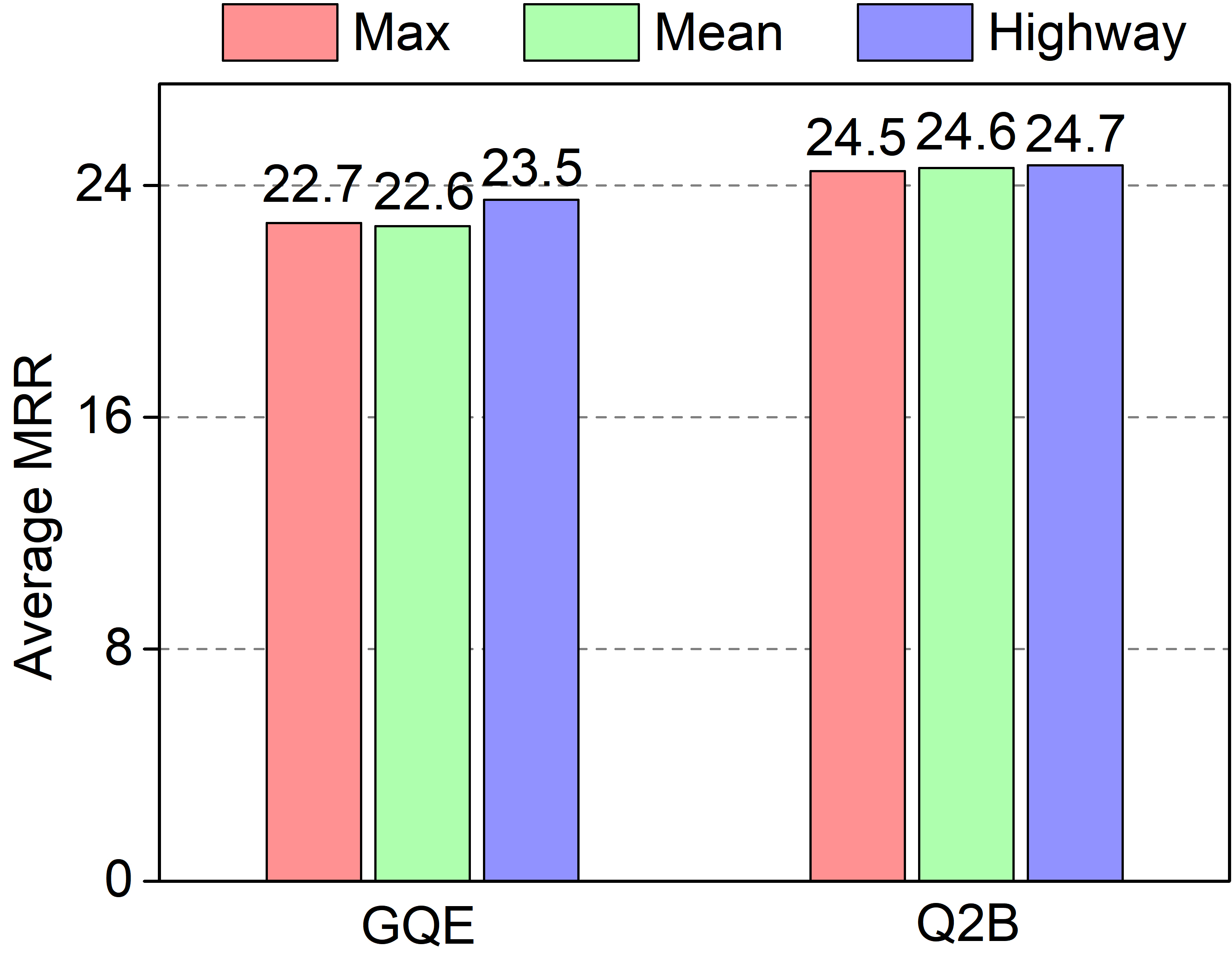
Figure 3: MRR results with different entity type aggregators.

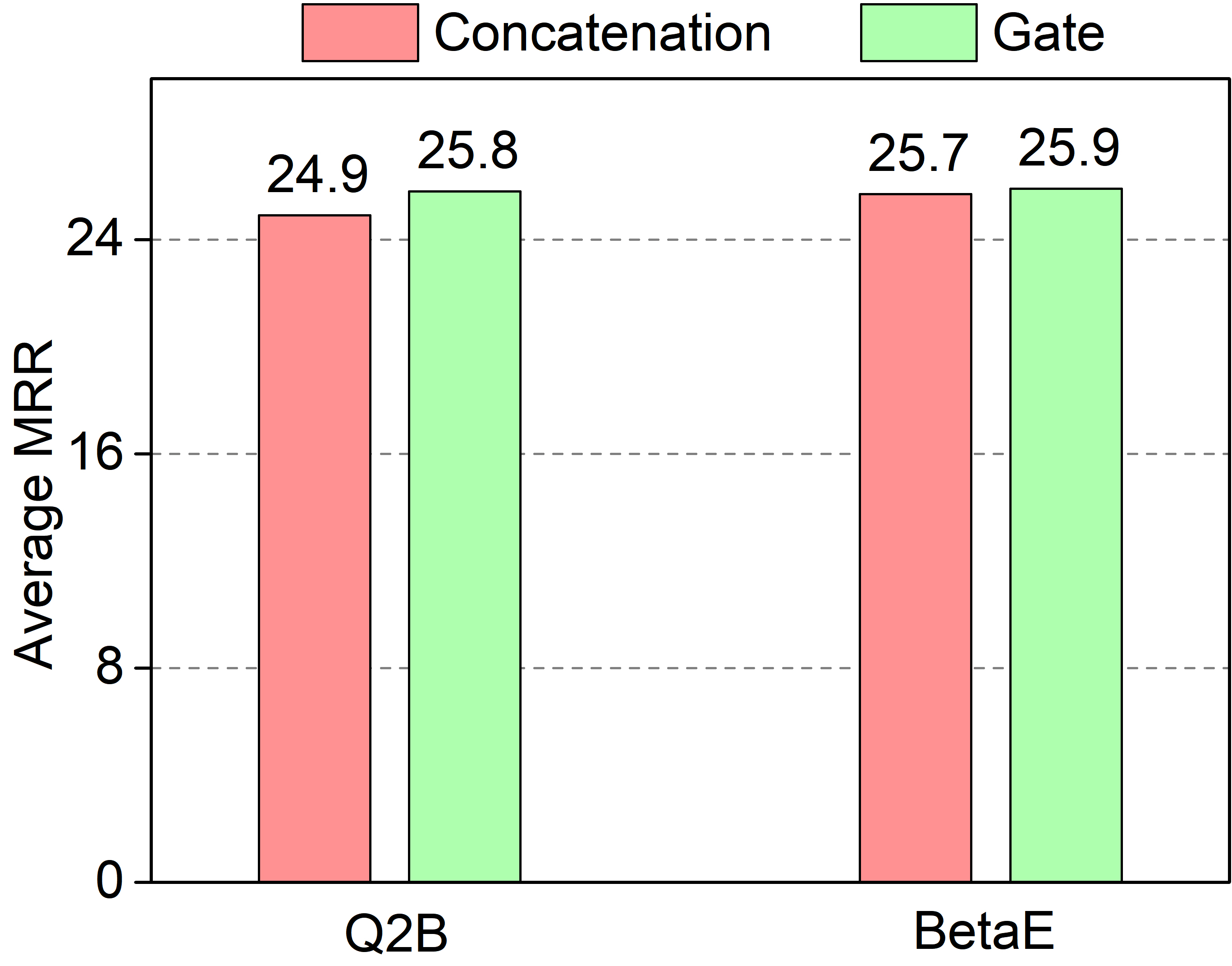
Figure 4: MRR results with different relation type aggregators.

Type-enhancement on relations is consistently better than on entities, this is explained by the fact that enhancing relation representations is more helpful for queries with long chains of existentially quantified variables as it better deals with cascading errors introduced by relation projections. We also show that using type-enhancement on both entities and relations usually leads to even better performance.

6 Conclusions

We proposed Temp, a type-aware plug-and-play model for answering FOL queries on incomplete KGs. We experimentally show that Temp can significantly improve four state-of-the-art models in terms of generalization, deductive and inductive reasoning abilities across three benchmark datasets consistently.

Appendix

	Queries	Training		Validation		Test
Reasoning Type	Datasets	1p/2p/3p/2i/3i	2in/3in/inp/pin/pni	1p	others	1p	others
Deductive Reasoning	FB15k	273,710	27,371	59,097	8,000	67,016	8,000
	FB15k-237	149,689	14,9,68	20,101	5,000	22,812	5,000
	NELL995	107,982	10,798	16,927	4,000	17,034	4,000
Inductive Reasoning	FB15k-237-V2	9,964	-	1,738	2,000	791	1,000
	NELL995-V3	12,010	-	2,197	2,000	1,167	1,500

Table 5: Number of training, validation, and test queries generated for different query structures on BetaE datasets. For Q2B datasets, except 2in/3in/inp/pin/pni, the remaining number of queries is consistent with the BetaE datasets. - denotes that we did not generate the query structures with negation operation for inductive reasoning.

A Details about Experiments

A.1 Datasets

For a fair comparison, we use the same datasets and query structures as in Q2B Ren et al. [2020] and BetaE Ren and Leskovec [2020]. For testing the inductive reasoning ability, we select GraIL Teru et al. [2020] providing datastes FB15k-237-V2 and NELL995-V3. We generate queries over these datasets following Ren and Leskovec [2020]. The statistics on the number of different queries in different datasets with different reasoning abilities can be found in Table 5.

A.2 Training Protocol

We run all the experiments on a single Tesla V100 32G GPU card. All the models are implemented in Pytorch. We adopt the original training objective and experimental parameters of each model. The best hyperparameters are shown in Table 6, note that we use the same parameters before and after adding Temp.

model	emb_dim	lr	batch_size	neg_size	margin
GQE	800	0.0001	512	128	24
Q2B	400	0.0001	512	128	24
BETAE	400	0.0001	512	128	60
LOGICE	400	0.0001	512	128	0.375

Table 6: emb_dim represents the embedding dimension, lr means the learning rate, neg_size is the negative sample size, and margin means the margin size.

A.3 Query Structures

Figure 5 shows the query structures on the BetaE datasets. The queries on the left of the black dotted line are used in the training phase. All fourteen queries in Figure 5 are used in both the validation and test phases. The queries within the green solid area are queries containing existential variable nodes. Unlike the BetaE datasets, the datasets provided by Q2B do not include query structures with negation operations (2in/3in/inp/pni/pin). We refer readers to the original Q2B and BetaE papers for technical details.

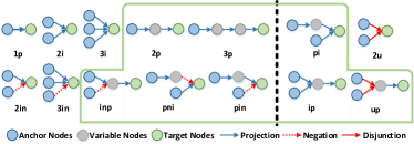
Figure 5: Fourteen queries considered in the experiments. Where ‘p’, ‘i’, ‘u’, and ‘n’ stand for ‘projection’, ‘intersection’, ‘union’, and ‘negation’, respectively.

A.4 Evaluation Metrics

The metrics Hit@K and MRR can be defined as follows:

$$\textit{Hits}@K(q)=\frac{1}{|A_{q}|}\sum_{v\in A_{q}}{\Phi(\textit{Rank}(v)\leq K)}$$ (11)

$$\textit{MRR}=\frac{1}{|A_{q}|}\sum_{v\in A_{q}}{\frac{1}{\textit{Rank}(v)}}$$ (12)

$A_{q}$ represents the answer set of q, Rank(v) denotes as the rank of v entity. $\Phi(\cdot)$ is an indicator function, when $x\leq K$, it equals to 1; 0 otherwise. Clearly, higher Hits@K and MRR indicate better prediction performance.

Generalization	Method	1p	2p	3p	2i	3i	pi	ip	2u	up	Avg
FB15k	GQE	54.6	15.3	10.8	39.7	51.4	27.6	19.1	22.1	11.6	28.0
	+Temp	74.9	31.4	26.0	59.3	69.4	47.3	35.9	47.8	27.4	46.6
	Q2B	68.0	21.0	14.2	55.1	66.5	39.4	26.1	35.1	16.7	38.0
	+Temp	74.8	25.6	22.3	61.7	72.6	43.7	29.0	44.1	22.5	44.0
	BetaE	65.1	25.7	24.7	55.8	66.5	43.9	28.1	40.1	25.2	41.6
	+Temp	70.3	28.9	25.8	58.2	68.4	45.8	32.2	44.3	27.3	44.6
	LogicE	72.3	29.8	26.2	56.1	66.3	42.7	32.6	43.4	27.5	44.1
	+Temp	74.9	30.9	27.3	58.3	68.2	43.8	33.8	46.1	28.9	45.8
FB15k-237	GQE	35.0	7.2	5.3	23.3	34.6	16.5	10.7	8.2	5.7	16.3
	+Temp	42.9	12.3	10.1	34.4	47.6	26.0	15.1	15.1	10.1	23.7
	Q2B	40.6	9.4	6.8	29.5	42.3	21.2	12.6	11.3	7.6	20.1
	+Temp	40.9	11.0	9.2	33.7	48.2	21.4	12.3	12.9	9.1	22.1
	BetaE	39.0	10.9	10.0	28.8	42.5	22.4	12.6	12.4	9.7	20.9
	+Temp	39.9	11.8	10.5	32.6	46.7	24.9	13.6	12.5	10.2	22.5
	LogicE	41.3	11.8	10.4	31.4	43.9	23.8	14.0	13.4	10.2	22.3
	+Temp	41.9	13.0	11.2	32.4	45.4	25.5	15.2	14.6	10.9	23.3
NELL	GQE	32.8	11.9	9.6	27.5	35.2	18.4	14.4	8.5	8.8	18.6
	+Temp	57.7	17.2	14.1	40.6	49.9	27.0	18.5	15.9	11.6	28.0
	Q2B	42.2	14.0	11.2	33.3	44.5	22.4	16.8	11.3	10.3	22.9
	+Temp	56.5	15.0	12.9	40.8	52.0	21.1	16.0	14.2	9.4	26.4
	BetaE	53.0	13.0	11.4	37.6	47.5	24.1	14.3	12.2	8.5	24.6
	+Temp	54.1	14.2	12.4	38.1	48.9	23.9	16.0	12.8	9.2	25.5
	LogicE	58.3	17.7	15.4	40.5	50.4	27.3	19.2	15.9	12.7	28.6
	+Temp	58.4	18.1	14.9	40.7	50.6	27.9	19.1	16.7	12.8	28.8

Table 7: Detailed MRR results on the BetaE’s datasets testing generalization.

Datasets	Methods	TER	TRR	1p	2p	3p	2i	3i	pi	ip	2u	up	Avg
FB15k	GQE	✖	✖	55.1	30.7	22.5	38.6	49.3	24.9	14.6	34.3	25.1	32.8
		✔	✖	65.3	38.1	29.4	52.1	64.3	35.5	17.9	44.6	31.4	42.1
		✖	✔	74.2	49.8	42.0	56.2	66.6	44.3	27.3	59.1	37.7	50.8
		✔	✔	75.2	50.4	42.0	56.9	67.1	44.5	28.2	59.5	34.0	50.9
	Q2B	✖	✖	68.3	39.0	28.5	52.2	64.0	37.4	20.1	50.6	30.1	43.4
		✔	✖	72.4	37.3	28.6	55.7	67.7	36.0	17.4	57.1	26.3	44.3
		✖	✔	69.9	46.1	38.8	56.2	68.6	41.8	25.6	52.7	29.3	47.7
		✔	✔	75.6	45.5	38.4	60.0	71.0	43.1	23.6	62.7	27.4	49.7
FB15k-237	GQE	✖	✖	35.0	19.2	14.4	22.1	31.4	14.5	8.8	14.8	14.5	19.4
		✔	✖	40.3	22.2	17.5	27.0	38.3	17.3	9.9	21.1	18.1	23.5
		✖	✔	43.9	26.8	22.5	28.2	37.6	20.4	11.9	24.9	20.9	26.3
		✔	✔	43.0	27.7	23.4	32.6	44.4	23.4	13.2	26.5	20.0	28.2
	Q2B	✖	✖	40.7	23.1	18.1	27.9	38.9	19.2	10.9	21.1	17.8	24.2
		✔	✖	42.1	23.1	17.6	29.6	41.3	18.1	9.9	22.7	17.7	24.7
		✖	✔	42.2	26.0	21.6	29.6	42.0	18.6	12.2	22.1	17.8	25.8
		✔	✔	41.2	25.8	21.9	33.1	45.0	21.0	11.4	24.4	17.7	26.8
NELL	GQE	✖	✖	31.3	18.2	16.8	22.4	30.4	15.8	10.0	16.8	12.1	19.3
		✔	✖	51.2	21.9	21.7	28.5	40.6	17.5	9.2	35.1	15.6	26.8
		✖	✔	55.5	31.8	31.7	33.6	46.1	23.0	14.1	38.9	24.4	33.2
		✔	✔	56.7	33.6	32.4	35.5	47.2	23.6	14.8	41.6	24.8	34.5
	Q2B	✖	✖	41.8	23.1	21.2	28.9	41.7	19.7	12.2	26.9	15.5	25.7
		✔	✖	54.4	22.9	23.0	33.7	47.4	15.9	10.1	38.7	15.8	29.1
		✖	✔	55.9	31.1	31.3	34.8	48.9	19.4	14.0	41.2	23.6	33.4
		✔	✔	57.1	31.9	31.3	36.6	49.5	19.4	13.5	41.7	23.8	33.9

Table 8: Detailed MRR results on the Q2B datasets with TER or TRR.

B Design Alternatives

In our ablation experiments, we test Temp with the following alternative models. In particular, when aggregating the type of an entity, we propose two alternatives for aggregator, instead of the highway aggregator in Eqs. (1), (2), and (3).

Mean aggregator.

$$\widetilde{\mathcal{H}_{s}^{K}}=\frac{1}{n}\sum_{i}\mathcal{H}_{s_{i}}^{K}$$ (13)

Here, the mean operation does not require a loop operation, so the value of K is 0. $\mathcal{H}_{s_{i}}^{K}\in\mathbb{R}^{d\times 1}$ represents the i-th component of the vector $\mathcal{H}_{s}^{K}\in\mathbb{R}^{d\times n}$.

Max aggregator.

$$\widetilde{\mathcal{H}_{s}^{K}}=\textit{Max}(\mathcal{H}_{s_{i}}^{K})$$ (14)

$\textit{Max}(\cdot)$ represents the element-wise maximum operation among the entity’s type information. K also takes 0.

Concatenation-based intersection.

Inspired by  liu2016learning and  reimers2019sentence, we apply an interactive concatenation to pair of the representations $\mathcal{G}^{er}$ and $\mathcal{G}^{es}$ in Eqs.(9) and (10), and then perform a linear layer operation. The interactive concatenation can be specified as:

$$\widetilde{\mathcal{G}^{e}}=W[\mathcal{G}^{er},\mathcal{G}^{es},\mathcal{G}^{er}+\mathcal{G}^{es},\mathcal{G}^{er}\times\mathcal{G}^{es}]+b,$$ (15)

where $+$ and $\times$ represent the element-wise addition and multiplication between two matrices $\mathcal{G}^{er}$ and $\mathcal{G}^{es}$, respectively. $[\cdot,\cdot,\cdot,\cdot]$ is used to concatenate the vector in row level.

C Additional Results

1. Table 7 shows detailed MRR results on the BetaE datasets, testing the generalization ability.

2. Table 8 shows detailed MRR results on the Q2B datasets with TER or TRR used separately or together.

3. Table 9 shows detailed Hits@3 results on the Q2B datasets about the generalization and deductive reasoning ability.

Generalization	Method	1p	2p	3p	2i	3i	pi	ip	2u	up	Avg
FB15k	GQE	71.7	36.1	25.9	47.5	60.8	30.0	15.8	45.2	28.1	40.1
	+Temp	83.0	54.6	46.0	64.1	74.8	50.0	30.8	68.7	37.3	56.6
	Q2B	82.1	43.0	31.7	62.7	74.5	44.4	22.4	66.7	33.5	51.2
	+Temp	84.0	49.8	42.2	67.4	77.9	48.3	26.1	72.7	30.0	55.4
	BetaE	75.0	45.1	40.0	62.2	75.4	47.1	22.3	58.9	29.6	50.6
	+Temp	79.5	50.2	44.3	63.7	74.4	48.8	27.4	64.5	30.0	53.6
	LogicE	80.5	50.5	45.8	62.2	72.5	47.5	28.3	63.9	36.8	54.2
	+Temp	83.2	51.5	46.4	64.0	73.8	47.8	28.6	69.0	36.9	55.7
FB15k-237	GQE	41.3	21.5	15.2	26.5	38.5	16.7	8.8	17.1	15.8	22.4
	+Temp	47.6	29.6	24.7	36.3	48.4	25.5	13.4	30.2	21.0	30.7
	Q2B	47.1	24.9	19.4	33.2	46.4	21.8	11.3	25.3	19.3	27.6
	+Temp	45.7	27.8	23.4	36.9	49.6	22.9	11.7	27.6	18.9	29.4
	BetaE	42.6	25.4	21.6	30.2	43.3	20.7	9.2	24.2	18.3	26.2
	+Temp	43.3	27.2	22.7	35.3	47.5	24.3	10.6	26.7	18.2	28.4
	LogicE	45.6	27.8	24.1	34.7	46.5	23.5	12.0	27.1	20.8	29.1
	+Temp	46.6	29.2	25.0	35.8	47.9	24.9	13.5	28.7	21.0	30.3
NELL	GQE	42.7	21.6	19.3	27.0	37.4	17.7	10.3	21.7	13.4	23.5
	+Temp	62.5	36.6	35.2	40.2	52.6	25.6	15.8	48.2	27.4	38.2
	Q2B	56.2	27.1	24.1	34.7	49.2	21.8	12.7	37.5	16.5	31.1
	+Temp	62.5	34.3	34.2	41.0	55.2	20.9	14.1	47.7	26.2	37.3
	BetaE	58.4	29.1	30.7	35.2	48.4	22.5	10.5	44.5	21.2	33.4
	+Temp	58.7	31.7	32.7	37.3	51.3	22.8	11.7	43.7	20.6	34.5
	LogicE	64.3	35.9	36.0	41.1	54.8	26.8	14.7	51.0	27.6	39.1
	+Temp	64.3	36.2	35.9	41.2	54.9	25.4	15.5	51.1	27.9	39.1
Deductive Reasoning	Method	1p	2p	3p	2i	3i	pi	ip	2u	up	Avg
FB15k	GQE	73.8	40.5	32.1	49.8	64.7	36.1	18.9	47.2	30.4	43.7
	+Temp	92.8	71.5	62.0	74.6	83.8	64.4	48.0	85.5	60.0	71.4
	Q2B	68.0	39.4	32.7	48.5	65.3	32.9	16.2	61.4	28.9	43.7
	+Temp	92.8	67.1	57.3	79.2	87.6	62.8	39.8	87.3	52.4	69.6
	BetaE	83.2	57.3	51.0	71.1	81.4	56.9	32.7	70.4	41.0	60.6
	+Temp	84.0	58.8	51.8	68.7	78.4	55.6	34.8	71.6	41.9	60.6
	LogicE	88.4	64.0	57.9	70.8	80.6	59.0	41.0	76.6	51.0	65.5
	+Temp	91.0	64.7	58.7	72.3	81.4	60.5	42.2	81.2	51.5	67.1
FB15k-237	GQE	56.4	30.1	24.5	35.9	51.2	25.1	13.0	25.8	22.0	31.6
	+Temp	76.3	48.6	39.0	49.7	60.4	36.9	22.1	59.0	36.3	47.6
	Q2B	58.5	34.3	28.1	44.7	62.1	23.9	11.7	40.5	22.0	36.2
	+Temp	87.2	59.6	47.9	67.2	72.7	49.1	29.8	78.6	43.4	59.5
	BetaE	77.9	52.6	44.5	59.0	67.8	42.2	23.5	63.7	35.1	51.8
	+Temp	84.7	58.3	49.4	62.3	68.8	45.3	28.5	74.5	41.4	57.0
	LogicE	81.5	54.2	46.0	58.1	67.1	44.0	28.5	66.6	40.8	54.1
	+Temp	84.5	59.8	51.9	59.3	68.1	47.0	33.4	70.8	45.4	57.8
NELL	GQE	72.8	58.0	55.2	45.9	57.3	34.2	24.8	59.0	40.7	49.8
	+Temp	93.3	84.1	73.3	73.4	81.4	60.8	45.8	90.3	76.8	75.5
	Q2B	83.9	57.7	47.8	49.9	66.3	29.6	19.9	73.7	31.0	51.1
	+Temp	98.3	95.4	86.0	92.2	95.2	86.1	69.5	98.5	92.8	90.4
	BetaE	94.3	88.2	76.2	84.0	90.2	68.8	46.6	92.5	81.4	80.2
	+Temp	95.1	89.8	79.5	83.3	89.3	69.0	51.1	93.0	83.3	81.5
	LogicE	96.2	90.7	84.1	84.1	89.5	76.0	65.2	94.7	87.1	85.3
	+Temp	96.5	91.0	83.2	82.7	88.9	72.6	64.1	95.2	86.9	84.6

Table 9: Detailed Hits@3 results on the Q2B datasets testing generalization and deductive reasoning.

References

- Arakelyan et al. [2021] Erik Arakelyan, Daniel Daza, Pasquale Minervini, and Michael Cochez. Complex query answering with neural link predictors. In ICLR, 2021.
- Bordes et al. [2013] Antoine Bordes, Nicolas Usunier, Alberto García-Durán, Jason Weston, and Oksana Yakhnenko. Translating embeddings for modeling multi-relational data. In NeurIPS, 2013.
- Chen et al. [2021] Jiajun Chen, Huarui He, Feng Wu, and Jie Wang. Topology-aware correlations between relations for inductive link prediction in knowledge graphs. In AAAI, pages 6271–6278, 2021.
- Choudhary et al. [2021a] Nurendra Choudhary, Nikhil Rao, Sumeet Katariya, Karthik Subbian, and Chandan Reddy. Probabilistic entity representation model for reasoning over knowledge graphs. In NeurIPS, 2021.
- Choudhary et al. [2021b] Nurendra Choudhary, Nikhil Rao, Sumeet Katariya, Karthik Subbian, and Chandan K Reddy. Self-supervised hyperboloid representations from logical queries over knowledge graphs. In WWW, 2021.
- Daza et al. [2021] Daniel Daza, Michael Cochez, and Paul Groth. Inductive entity representations from text via link prediction. In WWW, 2021.
- Hamilton et al. [2018] William L Hamilton, Payal Bajaj, Marinka Zitnik, Dan Jurafsky, and Jure Leskovec. Embedding logical queries on knowledge graphs. In NeurIPS, 2018.
- Luus et al. [2021] Francois Luus, Prithviraj Sen, Pavan Kapanipathi, Ryan Riegel, Ndivhuwo Makondo, Thabang Lebese, and Alexander Gray. Logic embeddings for complex query answering. In NeurIPS, 2021.
- Niu et al. [2020] Guanglin Niu, Bo Li, Yongfei Zhang, Shiliang Pu, and Jingyang Li. Autoeter: Automated entity type representation for knowledge graph embedding. In EMNLP, 2020.
- Pan et al. [2016] J.Z. Pan, G. Vetere, J.M. Gomez-Perez, and H. Wu. Exploiting Linked Data and Knowledge Graphs for Large Organisations. Springer, 2016.
- Pan et al. [2021] Weiran Pan, Wei Wei, and Xianling Mao. Context-aware entity typing in knowledge graphs. In EMNLP, 2021.
- Pan [2009] Jeff Z. Pan. Resource description framework. In Handbook on Ontologies, pages 71–90. 2009.
- Ren and Leskovec [2020] Hongyu Ren and Jure Leskovec. Beta embeddings for multi-hop logical reasoning in knowledge graphs. In NeurIPS, 2020.
- Ren et al. [2020] Hongyu Ren, Weihua Hu, and Jure Leskovec. Query2box: Reasoning over knowledge graphs in vector space using box embeddings. In ICLR, 2020.
- Srivastava et al. [2015] Rupesh Kumar Srivastava, Klaus Greff, and Jürgen Schmidhuber. Highway networks. arXiv preprint arXiv:1505.00387, 2015.
- Sun et al. [2020] Haitian Sun, Andrew O. Arnold, Tania Bedrax-Weiss, Fernando Pereira, and William W. Cohen. Faithful embeddings for knowledge base queries. In NeurIPS, 2020.
- Tai et al. [2015] Kai Sheng Tai, Richard Socher, and Christopher D. Manning. Improved semantic representations from tree-structured long short-term memory networks. In ACL, pages 1556–1566, 2015.
- Teru et al. [2020] Komal Teru, Etienne Denis, and Will Hamilton. Inductive relation prediction by subgraph reasoning. In ICML, pages 9448–9457, 2020.
- Toutanova and Chen [2015] Kristina Toutanova and Danqi Chen. Observed versus latent features for knowledge base and text inference. In ACL, pages 57–66, 2015.
- Wang et al. [2021] Hongwei Wang, Hongyu Ren, and Jure Leskovec. Relational message passing for knowledge graph completion. In SIGKDD, pages 1697–1707, 2021.
- Wiharja et al. [2020] Kemas Wiharja, Jeff Z. Pan, Martin J. Kollingbaum, and Yu Deng. Schema Aware Iterative Knowledge Graph Completion. Journal of Web Semantics, 2020.
- Xiong et al. [2017] Wenhan Xiong, Thien Hoang, and William Yang Wang. Deeppath: A reinforcement learning method for knowledge graph reasoning. In EMNLP, 2017.
- Yao et al. [2019] Liang Yao, Chengsheng Mao, and Yuan Luo. Kg-bert: Bert for knowledge graph completion. arXiv preprint arXiv:1909.03193, 2019.
- Zhang et al. [2020] Shuailiang Zhang, Hai Zhao, Yuwei Wu, Zhuosheng Zhang, Xi Zhou, and Xiang Zhou. Dcmn+: Dual co-matching network for multi-choice reading comprehension. In AAAI, 2020.
- Zhang et al. [2021] Zhanqiu Zhang, Jie Wang, Jiajun Chen, Shuiwang Ji, and Feng Wu. Cone: Cone embeddings for multi-hop reasoning over knowledge graphs. In NeurIPS, 2021.
- Zhao et al. [2020] Yu Zhao, Anxiang Zhang, Ruobing Xie, Kang Liu, and Xiaojie Wang. Connecting embeddings for knowledge graph entity typing. In ACL, 2020.