General approach of weak-to-strong measurement transition for Fock-state-based pointer states

Abstract

The transition from von Neumann’s projective strong measurement to Aharonov’s weak measurement has recently received large attention, theoretical and experimental. In this work, we present a general approach to describe the weak-to-strong measurement transition for Fock-state-based pointer states, and analyze in some details the case of coherent pointer states. A possible realization of our measurement scheme using trapped ions is also discussed.

I Introduction

Measurements are at the basis of physics, and represent the major tool for the quantitative understanding of our world. In quantum systems, the measurement problem has fostered a better understanding of quantum theory itself, and its applications to technology (Zurek, 2003; Haroche and J.-M.Raymond, 2006; Briegel et al., 2009; Taylor et al., 2013; Wiseman and Milburn, 2014; Matsuno, 2017; Wasielewski et al., 2020; Huggins et al., 2021). In standard textbooks, quantum measurements are usually introduced using the projective measurement model formulated by von Neumann (von Neumann J, 1955). The description of the Stern-Gerlach experiment is a typical example of this kind of measurement (Sakurai, 1993). This is a strong measurement model where the strength of the interaction between the pointer (measuring device) system and the measured one is strong enough to obtain the desired information about the measured system after a single trial, but the system itself collapses onto an eigenstate of the measured system observable. On the other hand, there is another type of measurement modelm proposed in 1988 by Aharonov et al (Aharonov et al., 1988). In this scheme, which also follows the basic requirements of von Neumann measurement theory, the coupling between the measured and the measuring systems is weak. As a consequence, the initially prepared system state is not destroyed after a single trial, and we still can get the required information statistically, after many repetitions (Tollaksen et al., 2010). In the weak measurement model, the value of the measured system observable is extracted in the form of weak value caused by the pre- and post-selection processes. This weak value is, in general, a complex number and different from the eigenvalue or expectation value of the corresponding system observable. Another important feature of weak values is that they could exceed the range of the eigenvalues. This feature is usually referred to as weak signal amplification and has been found useful in the solution of several problems in physics and related sciences (Hosten and Kwiat, 2008; Starling et al., 2009; Dixon et al., 2009; Lundeen et al., 2011; Pfeifer and Fischer, 2011; Lundeen and Bamber, 2012; Salvail et al., 2013; Boyd, 2013; Malik et al., 2013; Zhou et al., 2013; Di Lorenzo, 2013; Pan et al., 2019; Hariri et al., 2019; Denkmayr et al., 2017). For more details, the reader is referred to (Kofman et al., 2012; Malik et al., 2014) and the references therein.

In a recent study (Vaidman et al., 2017), it has been shown that the nature of weak values is different from that of the expectation values of the system observable, though weak values describe the interaction in the same way as the eigenvalue does. In general, a system observable is characterized by three sets of values: eigenvalues, (conditional) expectation values and weak values. The system information we want to obtain from the pointer after measurement is related to the pointer’s shifts. In order to get these values, we rely on different types of measurement models. The eigenvalues and the expectation values of the system observable are usually related to the position shift of the pointer after strong measurement. On the other hand, in the weak measurement procedures (Jozsa, 2007), the real and imaginary parts of weak values are obtained from the position and momentum shifts of the pointer, respectively.

As a matter of fact, a relevant point in von Neumann measurement model is that the coupling strength between the measured system and the pointer may assume arbitrary values, so that we can connect the weak and strong measurement schemes by adjusting it. Recently, the weak-to-strong measurement transition problems has been investigated experimentally (Pan et al., 2020) and theoretically (Araya-Sossa and Orszag, 2021; Turek et al., 2021) for some specific pointer states. However, a general approach to the weak-to-strong measurement transition for arbitrary pointer states has not been yet investigated.

In this paper, we present a general approach to describe the weak-to-strong measurement transition problem for infinite-dimensional (pure) pointer states in the Fock space, i.e. for the so-called Fock-state-based pointer states. We know that Fock number states $|n\rangle$ are the eigenstates of the number operator $\hat{n}=\hat{a}^{\dagger}\hat{a}$ , i.e., $\hat{a}^{\dagger}\hat{a}|n\rangle=n|n\rangle$. Thus, we can expand any quantum state $|\phi\rangle$ in the basis of $|n\rangle$ as $|\phi\rangle=\sum_{n}c_{n}|n\rangle$ with $c_{n}=\langle n|\phi\rangle$. We consider the internal (e.g. spin or polarization) and external degrees (e.g. spatial or field distribution) of freedom of the state as the measured system and pointer (measuring device), respectively, and give the general expressions of pointer shifts corresponding to the pointer position and momentum operators after measurement. Since these expressions are derived without any approximation, they are valid for any coupling, and we can described the transitions from Aharonov’s weak measurement to von Neumann’s projective strong measurement by tuning the coupling strength.

By using our general approach, the two extreme cases can be recovered, in which the shifted values of the pointers are directly associated with the conditional expectation values (strong measurement regime) and weak values (weak measurement regime), respectively. In particular, we derive a simple formula for the position shift of the pointer in the weak measurement regime and verify its agreement with previous results. We also analyze in some details the case of coherent state pointers by means of the Husimi-Kano $Q$ function in the phase space. Finally, we discuss the possible implementation of our transition measurement model in trapped ion systems.

The rest of this paper is organized as follows. In Sec. II, we provide a brief introduction to the von Neumann measurement by considering the weak and strong interaction cases. In Sec. IV, we derive the final pointer state of our weak-to-strong measurement transition model and present the general expressions of the position and momentum shifts. We also illustrate how to realize the weak-to-strong measurement transition by tuning the coupling strengths between the measured system and the pointer. We also verify our results by comparison with previous studies. In Sec.IV, as an example of our general approach, we investigate the coherent state based weak-to-strong measurement transition. In Sec. V, we discuss the possible experimental implementation of our model in trapped ion systems. In Sec. VI, we provide a brief summary of this paper. Throughout this paper, we use the unit $\hbar=1$.

II Brief introduction of quantum measurement

The overall Hamiltonian of our system is the sum of three terms $H=H_{s}+H_{p}+H_{int}$, where $H_{s}$ and $H_{p}$ denote the free Hamiltonians of the measured system and the pointer (measuring device), respectively, and $H_{int}$ is the interaction Hamiltonian between the system and pointer. In the following, since the readout information is related to the coupling between the system and the pointer, we describe the dynamics in an interaction picture and only consider the interaction Hamiltonian $H_{int}$. According to the von Neumann measurement theory, the general form of the interaction Hamiltonian can be written as (von Neumann J, 1955)

$$H_{int}=g(t)\hat{A}\otimes\hat{P},\text{\ \ $\int_{t_{0}}^{t}g(t)dt=g\delta(t-t_{0}).$}$$ (1)

Here, $\hat{A}$ is the system observable that we want to measure, whereas $\hat{P}$ represents the momentum operator of the pointer. The position operator $\hat{X}$ is its canonically cojugated operator, i.e. $[\hat{X},\hat{P}]=i$. The function $g(t)$ is nonzero only in a finite interaction time interval, and $g$ fully characterizes the coupling strength between the system and the pointer. If we denote by $|a_{i}\rangle$ and eigenstate of the observable $\hat{A}$ with the eigenvalue $a_{i}$, i.e., $\hat{A}|a_{j}\rangle=a_{j}|a_{j}\rangle$, then the observable $\hat{A}$ can be written as (Sakurai, 1993)

$$\hat{A}=\sum_{j}a_{j}|a_{j}\rangle\langle a_{j}|.$$ (2)

In general, given an observable $\hat{A}$, there are three sets of relevant values to be considered: the eigenvalues, the (conditional) expectation values, and the weak values. According to the measurement theory, these values can be obtained by a pointer’s shift after measurement. Since each eigenvalue is a special case of a (conditional) expectation values and weak values of the observable, we now provide a brief review of the readout procedures to obtain (conditional) expectation values and weak values.

1. Expectation value. Assume that the initial state of the pointer is $|\Phi\rangle$ with wave function $\Phi(x)$, and the measured system state is prepared in a superposition of eigenstates of $\hat{A}$, i.e., $|\psi_{i}\rangle=\sum_{j}\alpha_{j}|a_{j}\rangle$ with $\sum_{j}|\alpha_{j}|^{2}=\sum_{j}|\langle a_{j}|\psi_{j}\rangle|^{2}=1$. Under the action of the unitary evolution operator $e^{-ig\hat{A}\otimes\hat{P}}$, the total system state evolves into

$$|\Psi\rangle =e^{-ig\hat{A}\otimes\hat{P}}|\psi_{i}\rangle\otimes|\Phi(x)\rangle$$

$$=\sum_{j}\alpha_{j}|a_{j}\rangle\otimes|\Phi(x-ga_{j})\rangle.$$ (3)

The Eq. (3) implies that if a strong measurement of the observable $\hat{A}$ is performed with outcome $a_{j}$, then the wave function of the pointer collapses onto $\Phi(x-ga_{j})$, i.e. it is displaced by the amount $ga_{j}$ compared to the initial wave function $\Phi(x)$. After some algebra, the final position shift of the pointer for the strong measurement can be obtained as

$$\delta x_{st} ={\langle\Psi|\hat{X}|\Psi\rangle}-\langle\Phi|\hat{X}|\Phi\rangle$$

$$=g\langle A\rangle.$$ (4)

Here, $\langle A\rangle$ is the expectation value of the observable on the state $|\psi_{i}\rangle$, i.e.,

$$\langle A\rangle=\langle\psi_{i}|\hat{A}|\psi_{i}\rangle=\sum_{j}a_{j}|\alpha_{j}|^{2}.$$ (5)

This result can be esily understood by writing the initial density matrix

$$\rho =|\psi_{i}\rangle\langle\psi_{i}|$$

$$=\sum_{j}|\alpha_{j}|^{2}|a_{j}\rangle\langle a_{j}|+\sum_{j,k}\alpha_{j}\alpha_{k}^{\ast}|a_{j}\rangle\langle a_{k}|.$$ (6)

It is clear that $|\alpha_{i}|^{2}$ is the probability of eigenvalue $a_{i}$ of the observable $A$, corresponding to the eigenstate $|a_{i}\rangle$, if the system is prepared in $|\psi_{i}\rangle$. In order to obtain a determined outcome (i.e., an eigenvalue of the measured observable corresponding to a given eigenstate ), the second term (off-diagonal part which represented the coherence) of $\rho$ has to vanish after the measurement. This means that, after the measurement the system is a mixture of the eigenstates of the measured observable, i.e., $\sum_{j}P_{j}\rho P_{j}$, where $P_{j}=|a_{j}\rangle\langle a_{j}|$ are the projectors on the different eigenstates of $\hat{A}$. The disappearance of the off-dagonal terms in the above mixture is usually referred to as the projection postulate.

2. Conditional Expectation value. In time-symmetric quantum mechanics (Aharonov et al., 1964; Aharonov and Vaidman, 1991, 2008), if we assume that a postselection onto the state $|\psi_{f}\rangle=\sum_{j}\beta_{j}|a_{j}\rangle$ of $|\Psi\rangle$ [see Eq. (3)], is possible, than the unnormalized final state of the total system is given by

$$|\Psi^{\prime}\rangle=\sum_{j}\alpha_{j}\beta_{j}^{\ast}|a_{j}\rangle\otimes|\Phi(x-ga_{i})\rangle\,,$$ (7)

where $\sum_{j}|\beta_{j}|^{2}=\sum_{i}|\langle a_{i}|\text{$\psi_{f}$}\rangle|^{2}=1$. In this case, after the measurement the position shift of the pointer is proportional to the average value of the position operator

$$\delta x_{st} =\frac{\langle\Psi^{\prime}|\hat{X}|\Psi^{\prime}\rangle}{\langle\Psi^{\prime}|\Psi^{\prime}\rangle}-\langle\Phi|\hat{X}|\Phi\rangle=g\langle A\rangle_{c},$$ (8)

where $\langle A\rangle_{c}$ is the conditional expectation value of the observable $A$, and defined as (Aharonov et al., 1964)

$$\langle A\rangle_{c} =\frac{\sum_{j}a_{j}|\langle\psi_{f}|a_{j}\rangle\langle a_{j}|\psi_{i}\rangle|^{2}}{\sum_{k}|\langle\psi_{f}|a_{k}\rangle\langle a_{k}|\psi_{i}\rangle|^{2}}$$

$$=\frac{\sum_{j}a_{j}|\alpha_{j}\beta_{j}^{\ast}|^{2}}{\sum_{j}|\alpha_{j}\beta_{j}|^{2}}.$$ (9)

This value is also referred to a the postselected strong value of $\hat{A}$. In the above derivations, we have assumed that the coupling between the measured system and the pointer is strong enough to make the sub-wave-packets of the pointer corresponding to different eigenvalues distinguishable, i.e., $g\triangle a\gg\sigma$, where $\triangle a=a_{j}-a_{j-1}$ and $\sigma$ represent the differences of neighboring eigenvalues and the width of the sub-wave-packets, respectively.

3. Weak value. At variance with the situation considered above, if $g\triangle a\text{$<\sigma$}$, i.e., if system-pointer coupling is sufficiently weak, we cannot get the needed information after a single trial. In this case, we may consider the expansion of the unitary operator up to the first order term, such that the first line of Eq. (3) may be written as

$$|\eta\rangle\approx(1-ig\hat{A}\otimes\hat{P})|\psi_{i}\rangle\otimes|\Phi(x)\rangle.$$ (10)

As for the conditional strong measurement process, if we take a postselection on the state $|\psi_{f}\rangle$, then the (unnormalized) total system state may be written

$$|\eta^{\prime}\rangle \approx e^{-ig\langle A\rangle_{w}\hat{P}}|\psi_{f}\rangle\otimes|\Phi(x)\rangle$$

$$\propto|\psi_{f}\rangle\otimes\left|\Phi\left(x-gtRe\left[\langle A\rangle_{w}\right]\right)\right\rangle.$$ (11)

After the measurement, the position and momentum shifts of the pointer are given by (Jozsa, 2007)

$$\delta x_{w}\propto gRe\left[\langle A\rangle_{w}\right],$$ (12)

and

$$\delta p_{w}=2gIm\left[\langle A\rangle_{w}\right]Var\left(P\right),$$ (13)

respectively, where $Var\left(P\right)=\langle\Phi|P^{2}|\Phi\rangle-\langle\Phi|P|\Phi\rangle^{2}$ is the variance of the momentum operator $\hat{P}$ on the initial pointer state, and $\langle A\rangle_{w}$ is the weak value, which is defined as

$$\langle A\rangle_{w} =\frac{\langle\psi_{i}|\hat{A}|\psi_{f}\rangle}{\langle\psi_{i}|\psi_{f}\rangle}=\frac{\sum_{j}\sum_{k}\alpha_{j}\beta_{k}^{\ast}\langle a_{k}|\hat{A}|a_{j}\rangle}{\sum_{j}\sum_{k}\alpha_{j}\beta_{k}^{\ast}\langle a_{k}|a_{j}\rangle}$$

$$=\frac{\sum_{j}a_{j}\alpha_{j}\beta_{j}^{\ast}}{\sum_{j}\alpha_{j}\beta_{j}^{\ast}}\,,$$ (14)

where, $Re[c]$ and $Im[c]$ denote the real and the imaginary parts of the complex number $c$, respectively. In general, the conditional expectation value $\langle A\rangle_{c}$ and the weak value $\langle A\rangle_{w}$ are different [see Eqs. (9) and (14) ], and thus correspond to different measurement strengths (Ban, 2015). In other words, the (conditional) expectation value of system observable is related to the (postselected) strong measurement, while the weak value is caused by the postselected weak measurement. In can be easily seen that if $\beta_{i}=\alpha_{i},$ the conditional expectation value and the weak value reducedto the expectation value given in Eq. (5). As shown above, these values can be obtained from the position shifts of the pointer after the measurement.

III General Approach to the weak-to-strong measurement transition

In some recent studies, the weak-to-strong measurement transition has been investigated theoretically and experimentally by using some specific pointer state (Pan et al., 2020; Araya-Sossa and Orszag, 2021). However, a general approach to this problem has not been presented yet. In this section, we provide a general approach based on the measurement scheme illustrated in Fig. 1. We know that the Fock number states are the eigenstates of the number operator $\hat{n}=\hat{a}^{\dagger}\hat{a}$, i.e., $\hat{a}^{\dagger}\hat{a}|n\rangle=n|n\rangle$. One can expand any state in the basis of $|n\rangle$ since the number operator is Hermitian. In other words, any state $|\phi\rangle$ can be written as:

$$|\phi\rangle=\sum_{n}c_{n}|n\rangle,$$ (15)

where the expansion coefficients $c_{n}$ are determined by $c_{n}=\langle n|\phi\rangle$. Let us assume that the pointer and the measured system are prepared in the states $|\phi\rangle$ and $|\psi_{i}\rangle,$ respectively. Then the total initial state can be written as $|\phi\rangle\otimes|\psi_{i}\rangle$ and the evolution of the total system is generated by the interaction Hamiltonian given in Eq. (1) as

$$|\Psi_{evol}\rangle =\exp\left(-i\int_{0}^{t}H_{int}(\tau)d\tau\right)|\psi_{i}\rangle\otimes|\phi\rangle$$

$$=\sum_{i}\alpha_{i}D\left(\frac{\Gamma}{2}a_{i}\right)|a_{i}\rangle\otimes|\phi\rangle$$

$$=\sum_{n,i}\alpha_{i}c_{n}|a_{i}\rangle\otimes\left|\frac{\Gamma}{2}a_{i},n\right\rangle,$$ (16)

where

$$D\left(\frac{\Gamma}{2}a_{i}\right)=\exp\left(\frac{g}{2\sigma}a_{i}(a^{\dagger}-a)\right),\ \ \ \Gamma=\frac{g}{\sigma}$$ (17)

is the displacement operator, and

$$\left|\frac{\Gamma}{2}a_{i},n\right\rangle=D\left(\frac{\Gamma}{2}a_{i}\right)|n\rangle$$ (18)

is usually referred to as displaced Fock states. In the derivation of Eq. (16), we used the expression of the pointer momentum operator $\hat{P}$ in terms of the annihilation and creation operators $\hat{a}$ and $\hat{a}^{\dagger}$as

$$\hat{P}=\frac{i}{2\sigma}\left(\hat{a}^{\dagger}-\hat{a}\right).$$ (19)

The parameter $\Gamma=g/\sigma$ characterizes the coupling strength between the measured system and the pointer. If $\Gamma\gg 1$ ($\Gamma\ll 1$), the measurement is in the strong (weak) measurement regime. After a postselection onto the state $|\psi_{f}\rangle$ the normalized final state of the pointer reads as follows

$$|\varTheta\rangle=\mathcal{N}\sum_{i}\sum_{n}\alpha_{i}\beta_{i}^{\ast}c_{n}\left|\frac{\Gamma}{2}a_{i},n\right\rangle,$$ (20)

where $\mathcal{N}$ is a normalization coefficient given by

$$\mathcal{N}^{-2} =\sum_{i,j}\sum_{n,m}c_{m}^{\ast}c_{m}\alpha_{j}^{\ast}\beta_{j}\alpha_{i}\beta_{i}^{\ast}L_{n}\left(\frac{\Gamma^{2}}{4}|a_{i}-a_{j}|^{2}\right)\times$$

$$\exp\left[-\frac{\Gamma^{2}}{8}|a_{i}-a_{j}|^{2}\right]$$

$$=\sum_{i}|\alpha_{i}\beta_{i}^{\ast}|^{2}+\sum_{n}\sum_{i\neq j}\alpha_{j}^{\ast}\beta_{j}\alpha_{i}\beta_{i}^{\ast}|c_{n}|^{2}L_{n}\left(\frac{\Gamma^{2}}{4}|a_{i}-a_{j}|^{2}\right)\times$$

$$\exp\left[-\frac{\Gamma^{2}}{8}|a_{i}-a_{j}|^{2}\right],$$ (21)

where $L_{n}(x)$ denote the n-th Laguerre polynomials. Eq. (20) contains the information about the system observable $A$ that we want to measure, and holds for all Fock-state-based pointer states. In the next subsection, we derive the general formulas of pointer shifts and discuss the weak-to-strong measurement transition.

          

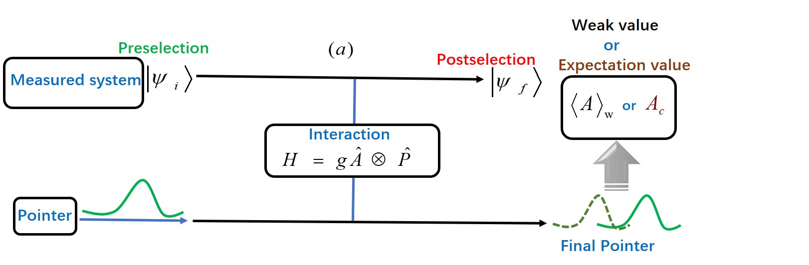
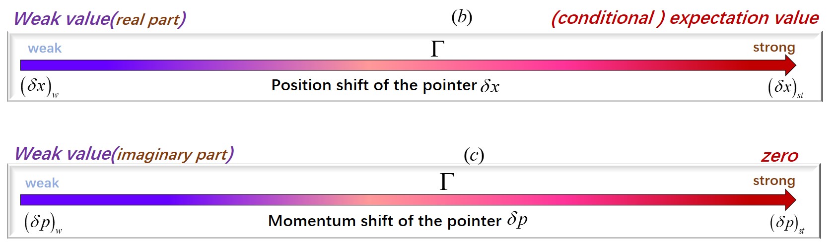
Figure 1: Schematic diagram of our scheme to realize weak-to-strong measurement transition . Panel (a) shows the postselected von Neumann measurement model; (b) and (c) show the relationships between the shifts of the pointer and the values of the associated system observable.

III.1 Position shift

Here, we give the general expression of the position shift of the Fock-state-based pointer states after the postselected von Neumann measurement. The position operator $\hat{X}$ of the pointer can be written in term of annihilation and creation operators $\hat{a}$ and $\hat{a}^{\dagger}$as

$$\hat{X}=\sigma\left(\hat{a}^{\dagger}+\hat{a}\right).$$ (22)

Since the interaction causes the shifts of the pointer, we can read the system information by comparing the pointer state before and after the measurement. For our scheme, the position shift of the pointer after the postselected von Neumann measurement reads as

$$\delta x =\langle\varTheta|\hat{X}|\varTheta\rangle-\langle\phi|\hat{X}|\phi\rangle$$

$$=\mathcal{|N}|^{2}\sigma\sum_{i,j}\sum_{n,m}c_{m}^{\ast}c_{n}\alpha_{j}^{\ast}\beta_{j}\alpha_{i}\beta_{i}^{\ast}$$

$$\text{$\times$}\{\sqrt{n+1}\langle m|D\left[\frac{\Gamma}{2}\left(a_{i}-a_{j}\right)\right]|n+1\rangle$$

$$+\sqrt{n}\langle m|D\left[\frac{\Gamma}{2}\left(a_{i}-a_{j}\right)\right]|n-1\rangle+$$

$$\Gamma a_{i}\langle m|D\left[\frac{\Gamma}{2}\left(a_{i}-a_{j}\right)\right]|n\rangle\}-\langle\phi|\hat{X}|\phi\rangle,$$ (23)

where

$$\langle\phi|\hat{X}|\phi\rangle=2\sigma\sum_{n}\sqrt{n+1}Re\left[c_{n}c_{n+1}^{\ast}\right]$$ (24)

is the initial average value of the position operator on the initial pointer state $|\phi\rangle$. The explicit forms of the matrix elements of displacement operator in the above formula are given by (de Oliveira et al., 1990)

$$\langle m|D\left(\alpha\right)|n\rangle$$

$$=e^{-\frac{|\alpha|^{2}}{2}}\begin{cases}\sqrt{\frac{n!}{m!}}L_{n}^{m-n}\left(|\alpha|^{2}\right)\left(\alpha\right)^{m-n},&m\geq n\\ \sqrt{\frac{m!}{n!}}L_{m}^{n-m}\left(|\alpha|^{2}\right)\left(\alpha\right)^{n-m}.&m\leq n\end{cases}$$ (25)

where the generalized Laguerre polynomials are defined as

$$L_{n}^{(\eta)}(x)=\sum_{k=0}^{n}\left(\begin{array}[]{c}n+\eta\\ n-k\end{array}\right)\frac{(-1)^{k}}{k!}x^{k}.$$ (26)

Eq. (23) is the general expression of the position shift of the Fock- state-based pointer measurement schemes, and it holds in all measurement regimes.

If one wants to know the position shift of the pointer in the postselected strong measurement regime, then one can consider larger values of the coupling $\Gamma$. In order to do that, a limit $\Gamma\rightarrow\infty$ should be taken to Eq. (23 ) which gives

$$\left(\delta x\right)_{st} =\lim_{\Gamma\rightarrow\infty}\delta x$$

$$= \frac{\text{$\sigma$}}{\sum_{i}|\alpha_{i}\beta_{i}^{\ast}|^{2}}\{\sum_{i}\sum_{n,m}c_{m}^{\ast}c_{n}|\alpha_{i}\beta_{i}^{\ast}|^{2}\times$$

$$\left(\sqrt{n+1}\delta_{m,n+1}+\sqrt{n}\delta_{m,n-1}+\Gamma a_{i}\delta_{m,n}\right)\}$$

$$-\langle\phi|\hat{X}|\phi\rangle$$

$$=g\frac{\sum_{i}a_{i}|\alpha_{i}\beta_{i}^{\ast}|^{2}}{\sum_{i}|\alpha_{i}\beta_{i}^{\ast}|^{2}}=g\langle A\rangle_{c}.$$ (27)

In the above expression, $\delta_{m,n}$ represents the Kronecker delta function

$$\delta_{m,n}=\begin{cases}1,&m=n\\ 0,&m\neq n\end{cases}$$ (28)

Eq. (27) is the position shift formula for the postselected strong von Neumann measurement introduced in Sec. II. On the other hand, if we are interested in the postselected weak measurement, $\Gamma$ should be set vanishingly small. In this case, the position shift of the pointer reads as follows

$$\left(\delta x\right)_{w} =\lim_{\Gamma\rightarrow 0}\delta x$$

$$=gtRe\left[\langle A\rangle_{w}\right]+2gtIm\left[\langle A\rangle_{w}\right]\times$$

$$\{Im\left[\sum_{n}\sqrt{(n+1)(n+2)}c_{n}^{\ast}c_{n+2}\right]$$

$$-Im\left[\sum_{n}\sqrt{n+1}c_{n}^{\ast}c_{n+1}\right]^{2}\}$$

$$=gRe\left[\langle A\rangle_{w}\right]+2gIm\left[\langle A\rangle_{w}\right]Im\left[\langle a^{2}\rangle-\langle a\rangle^{2}\right].$$ (29)

Eq. (29) is the concise form of the expression presented in (Dressel and Jordan, 2012). It gives the position shift of the pointer in posteselectd weak measurement, and holds for any pointer state that can be written in Fock state basis. In the above position shift formula, $\langle a\rangle$ ($\langle a^{2}\rangle$) denotes the expectation value of the annihilation operator $a$ (squared annihilation operator $a$) in the initial pointer state $|\phi\rangle$.

Let us now exploit Eq. (29) to investigate the transition for some specific pointer state, which have been investigated in recent studies cite those studies here? (1) Coherent state. If we assume that the pointer is initially prepared in a coherent state, i.e., $|\phi\rangle=|\alpha\rangle=\sum_{n}c_{n}|n\rangle$ with $c_{n}=e^{-\frac{|\alpha|^{2}}{2}}\frac{\alpha^{n}}{\sqrt{n!}}$, then

$$\langle a^{2}\rangle_{ch}=\langle\alpha|a^{2}|\alpha\rangle=\alpha^{2},\ \ \ \langle\alpha|a|\text{$\alpha\rangle=\alpha$ .}$$ (30)

In this case the position shift, Eq. (29), is given by

$$\left(\delta x\right)_{w,coh}=gRe\left[\langle A\rangle_{w}\right].$$ (31)

This result coincides with that presented in Ref. (Turek et al., 2015; Xu et al., 2022).

(2) Coherent squeezed state. Assuming the pointer initially prepared in a coherent squeezed state, we recover the results of Ref. (Araya-Sossa and Orszag, 2021) by using Eq. (29). Squeezed coherent states are defined as $|\phi\rangle=|\alpha,\xi\rangle=D(\alpha)S(\xi)|0\rangle$ where

$$D(\alpha)=\exp\left(\alpha a^{\dagger}-\alpha^{\ast}a\right),S(\xi)=\exp\left(\frac{1}{2}\xi^{\ast}a^{2}-\frac{1}{2}\xi a^{\dagger 2}\right).$$ (32)

Here, $D(\alpha)$ and $S(\xi)$ are the displacement and squeezed operator, respectively, with $\alpha=|\alpha|e^{i\phi_{\alpha}}$ and $\xi=re^{i\phi_{\xi}}$. This state also can be written in terms of Fock state basis as (Gerry and Knight, 2005)

$$|\alpha,\xi\rangle=\sum_{n}c_{n}|n\rangle,$$ (33)

where

$$c_{n} =\frac{1}{\sqrt{\cosh r}}\exp\left[-\frac{|\alpha|^{2}}{2}-\frac{1}{2}\alpha^{\ast 2}e^{i\phi_{\xi}}\tanh r\right]$$

$$\times\sum_{n=0}^{\infty}\frac{\left[\frac{1}{2}e^{i\phi_{\xi}}\tanh r\right]^{n/2}}{\sqrt{n!}}H_{n}\left[\gamma\left(e^{i\phi_{\xi}}\sinh(2r)\right)^{-\frac{1}{2}}\right]$$ (34)

with $\gamma=\alpha\cosh r+\alpha^{\ast}e^{i\phi_{\xi}}\sinh r$, and $H_{n}(x)$ being the the order $n$ Hermite polynomial. The expectation value of $\langle a\rangle$ and $\langle a^{2}\rangle$ under the state $|\alpha,\xi\rangle$ are given as

$$\langle a\rangle_{sc}=\alpha,\ \ \ \langle a^{2}\rangle_{sc}=\alpha^{2}-e^{i\phi_{\xi}}\sinh r\cosh r.$$ (35)

In this case, after the postselected weak measurement, the position shift of the pointer reads as

$$\left(\delta x\right)_{w,sc} =gRe\left[\langle A\rangle_{w}\right]-gIm\left[\langle A\rangle_{w}\right]\sinh 2r\sin\phi_{\xi}.$$ (36)

This is the same result derived in Ref. (Araya-Sossa and Orszag, 2021) for squeezed coherent pointer.

(3) Single-photon-added coherent state(SPAC). The SPAC state is defined as (Agarwal and Tara, 1991)

$$|1,\alpha\rangle=\sum_{n}c_{n}|n+1\rangle$$ (37)

where

$$c_{n}=\frac{e^{-\frac{|\alpha|^{2}}{2}}}{\sqrt{1+|\alpha|^{2}}}\sqrt{\frac{n+1}{n!}}.$$ (38)

The expectation values $\langle a\rangle_{spac}$ and $\langle a^{2}\rangle_{spac}$ for the state $|1,\alpha\rangle$ are given by

$$\langle a\rangle_{spac}=\frac{\alpha(2+|\alpha|^{2})}{1+|\alpha|^{2}},$$ (39)

and

$$\langle a^{2}\rangle_{spac}=\frac{\alpha^{2}(3+|\alpha|^{2})}{1+|\alpha|^{2}},\ \ \ \$$ (40)

respectively. Thus, if we take the pointer initially prepared in a SPAC state, its position shift after the postselected weak measurement would be shifted by

$$\left(\delta x\right)_{w,spac}=gRe\left[\langle A\rangle_{w}\right]-2g\frac{|\alpha|^{2}\sin 2\phi_{\alpha}}{\left(1+|\alpha|^{2}\right)^{2}}Im\left[\langle A\rangle_{w}\right].$$ (41)

This is the same result obtained in Ref. (Xu et al., 2022; Turek et al., 2021). From the above examples it can be confirmed that the Eq. ( 29) can be used for any pointer states.

III.2 Momentum shift

The shifts in the momentum of the pointer may be evaluated in a similar way. After a postselected von Neumann measurement we have

$$\delta p =\langle\varTheta|\hat{P}|\varTheta\rangle-\langle\phi|\hat{P}|\phi\rangle$$

$$=\frac{i}{2\sigma}\mathcal{|N}|^{2}\sum_{i,j}\sum_{n,m}c_{m}^{\ast}c_{n}\alpha_{j}^{\ast}\beta_{j}\alpha_{i}\beta_{i}^{\ast}$$

$$\times\{\sqrt{n+1}\langle m|D\left[\frac{\Gamma}{2}\left(a_{i}-a_{j}\right)\right]|n+1\rangle$$

$$-\sqrt{n}\langle m|D\left[\frac{\Gamma}{2}\left(a_{i}-a_{j}\right)\right]|n-1\rangle\}-\langle\phi|\hat{P}|\phi\rangle\,,$$ (42)

where

$$\langle\phi|\hat{P}|\phi\rangle=\frac{1}{\sigma}Im\left[\sum_{n}\sqrt{n+1}c_{n+1}^{\ast}c_{n}\right]$$ (43)

is the expectation value of the momentum operator in the initial pointer state $|\phi\rangle.$ No approximation has been used to derive Eq. ( 42), and thus it provides the momentum shift of the pointer in all measurement regimes. Again, the two extremes give the momentum shifts corresponding to the strong and weak measurement, respectively: (i) For a very strong coupling ($\Gamma\gg 1)$, corresponding to the strong measurement regime, the momentum shift becomes

$$\left(\delta p\right)_{st} =\lim_{\Gamma\rightarrow\infty}\delta p$$

$$=\frac{i}{2\sigma\sum_{j}|\alpha_{i}\beta_{i}|^{2}}\sum_{i,j}\sum_{n,m}c_{m}^{\ast}c_{n}\alpha_{j}^{\ast}\beta_{j}\alpha_{i}\beta_{i}^{\ast}$$

$$\times\{\sqrt{n+1}\langle m|D\left[\frac{\Gamma}{2}\left(a_{i}-a_{j}\right)\right]|n+1\rangle$$

$$-\sqrt{n}\langle m|D\left[\frac{\Gamma}{2}\left(a_{i}-a_{j}\right)\right]|n-1\rangle\}-\langle\phi|\hat{P}|\phi\rangle$$

$$=\frac{i}{2\sigma}\sum_{n,m}c_{m}^{\ast}c_{n}\{\sqrt{n+1}\langle m|n+1\rangle-\sqrt{n}\langle m|n-1\rangle\}$$

$$-\frac{1}{\sigma}Im\left[\sum_{n}\sqrt{n+1}c_{n+1}^{\ast}c_{n}\right]=0.$$ (44)

(ii) On the contrary, in the weak measurement regime ($\Gamma\ll 1$), we get

$$\left(\delta p\right)_{w} =\lim_{\Gamma\rightarrow 0}\delta p$$

$$=\frac{i}{2\text{$\sigma\sum_{i,j}\alpha_{j}^{\ast}\beta_{j}\alpha_{i}\beta_{i}^{\ast}$}}\sum_{i,j}\sum_{n,m}c_{m}^{\ast}c_{n}\alpha_{j}^{\ast}\beta_{j}\alpha_{i}\beta_{i}^{\ast}$$

$$\times\{\sqrt{n+1}\langle m|D\left[\frac{\Gamma}{2}\left(a_{i}-a_{j}\right)\right]|n+1\rangle$$

$$-\sqrt{n}\langle m|D\left[\frac{\Gamma}{2}\left(a_{i}-a_{j}\right)\right]|n-1\rangle\}-\langle\phi|\hat{P}|\phi\rangle$$

$$=2gIm\left[\langle A\rangle_{w}\right]\left(\langle\hat{P}^{2}\rangle-\langle\hat{P}\rangle^{2}\right)$$

$$=2gIm\left[\langle A\rangle_{w}\right]Var(P).$$ (45)

where $Var(P)$ is the variance of the momentum operator $\hat{P}$ in the initial pointer state $|\phi\rangle$. The final results of Eq. (44) and Eq. (45) agree with those contained in previous works (Araya-Sossa and Orszag, 2021; Jozsa, 2007; Turek et al., 2021), and holds for any pointer states.

IV Example: coherent state pointer case

IV.1 Measurement transition

As an example of application of our general method to described the weak-to-strong measurement transition, we here consider a pointer state initially prepared in a coherent state. We assume that the interaction Hamiltonian between the measured system and the pointer has the form (1), and the system observable $\hat{A}$ is the Pauli-$x$ operator, i.e., $\hat{A}=\hat{\sigma}_{x}=|+\rangle\langle+|+|-\rangle\langle-|$. Here, $|\pm\rangle\equiv\left(|\uparrow\rangle\pm|\downarrow\rangle\right)/\sqrt{2}$ are the eigenstates of $\hat{\sigma}_{x}$ with eigenvalues $\pm 1$, respectively. If we assume that the measured system is initially prepared in the state $|\psi_{ini}\rangle=|\downarrow\rangle$, and pointer is prepared in coherent state $|\phi(x)\rangle=|\beta\rangle$ with $\beta=re^{i\varphi}$, then the initial total state of the system can be written as $|\downarrow\rangle\otimes|\beta\rangle$. Given the unitary operator $U=e^{-ig\hat{\sigma}_{x}\otimes\hat{P}}$, the total system state given in Eq. (16) evolves as

$$|\Omega\rangle =\frac{1}{\sqrt{2}}\left[|+\rangle D\left(\frac{\Gamma}{2}\right)|\beta\rangle-|-\rangle D^{\dagger}\left(\frac{\Gamma}{2}\right)|\beta\rangle\right],$$ (46)

with $\Gamma=\frac{g}{\sigma}.$ If we take a postselection onto the state $|\psi_{f}\rangle=\cos\theta|\uparrow\rangle-\sin\theta|\downarrow\rangle$, then the final state of the pointer [see Eq. (20] reduces to

$$|\Psi^{\prime\prime}\rangle=$$

$$\frac{\sin\left(\frac{\pi}{4}-\theta\right)e^{-i\frac{\Gamma}{2}r\sin\varphi}|\beta+\frac{\Gamma}{2}\rangle-\cos\left(\frac{\pi}{4}-\theta\right)e^{i\frac{\Gamma}{2}r\sin\varphi}|\beta-\frac{\Gamma}{2}\rangle}{\sqrt{1-\cos\left(2\theta\right)\cos\left(2\Gamma r\sin\varphi\right)e^{-\frac{1}{2}\Gamma^{2}}}}.$$ (47)

As we can see, this is a superposition of two coherent states with different coherent amplitudes. In the $x$-representation the state $|\Psi^{\prime}\rangle$ can be expressed as

$$\Psi^{\prime\prime}(x) =\langle x|\Psi^{\prime\prime}\rangle=$$

$$\frac{\sin\left(\frac{\pi}{4}-\!\!\theta\right)e^{-i\frac{\Gamma}{2}r\sin\varphi}\psi_{+}(x)\!-\!\cos\left(\frac{\pi}{4}-\!\!\beta\right)e^{i\frac{\Gamma}{2}r\sin\varphi}\psi_{-}(x)}{\sqrt{1-\cos\left(2\theta\right)\cos\left(2\Gamma r\sin\varphi\right)e^{-\frac{1}{2}\Gamma^{2}}}},$$ (48)

where

$$\psi_{\pm}(x) =\langle x|\beta\pm\frac{\Gamma}{2}\rangle$$

$$=\left(\frac{1}{2\pi\sigma^{2}}\right)^{\frac{1}{4}}e^{-|\beta\pm\frac{\Gamma}{2}|^{2}}$$

$$\times\exp\left(\frac{x^{2}}{4\sigma^{2}}\right)\exp\left[-\frac{\left(x-\sigma(\beta\pm\frac{\Gamma}{2})\right)^{2}}{2\sigma^{2}}\right]$$ (49)

are Gaussian wave packets with central position shifts $\pm\frac{\Gamma}{2}$ compared to the initial Gaussian caused by the interaction with the measured system. On the other hand, for our pre- and postselected states $|\downarrow\rangle$ and $\cos\theta|\uparrow\rangle-\sin\theta|\downarrow\rangle$ , the corresponding conditional expectation value and weak value defined in Eq. (9) and Eq. (14) can be written as

$$\langle\sigma_{x}\rangle_{c}=-\sin(2\theta),$$ (50)

and

$$\langle\sigma_{x}\rangle_{w}=-\cot(\theta),$$ (51)

respectively. As we show in the following, the conditional expectation value $\langle\sigma_{x}\rangle_{c}$ and weak value $\langle\sigma_{x}\rangle_{w}$ are directly related to the pointer shifts of strong postselected measurement and postselected weak measurement, respectively.

Position shift. We can check the weak-to-strong measurement transition by investigating the position and momentum shifts of the pointer after measurement. As mentioned in Sec. II, the the parameter $\Gamma$ quantifies the measurement strength and it can takes all values, thus realizing a weak-to-strong transition. The general expression of the position shift after postselected von Neumann measurement for coherent pointer state, can be calculated by using Eq. (48). We hav

$$\delta x_{coh} =\langle x\rangle_{fi}-\langle x\rangle_{ini}$$

$$=\frac{-\text{$g$$\sin$$(2\theta)$}+\frac{1}{2}gr\cos\varphi\cos\left(2\theta\right)\cos\left(2\Gamma r\sin\varphi\right)e^{-\frac{1}{2}\Gamma^{2}}}{1-\cos\left(2\theta\right)\cos\left(2\Gamma r\sin\varphi\right)e^{-\frac{1}{2}\Gamma^{2}}}.$$ (52)

It is straightforward to see from this expression that the measurement transition can be controlled by adjusting $\Gamma$ in the term $e^{-\frac{1}{2}\Gamma^{2}}$. To get the position shift of the coherent state pointer after a strong measurement, we take the limit of Eq. (52) for $\Gamma$ goes to infinity, i.e.,

$$\left(\delta x\right)_{strong} =\lim_{\Gamma\rightarrow\infty}\delta x_{coh}=-g\text{$\sin$$(2\theta)$}=g\langle\sigma_{x}\rangle_{c}.$$ (53)

This result exactly matches with the Eq. (27). Taking the opposite limit, i.e., $\Gamma\ll 1$, we go to weak measurement regime and pointer shift position becomes

$$\left(\delta x\right)_{weak} =\lim_{\Gamma\rightarrow 0}\delta x_{coh}=-g\cot\theta=g\langle\sigma_{x}\rangle_{w}.$$ (54)

This result validates again Eq. ( 29). In order to explore the weak-to-strong measurement transition, as characterized by the position shift of the coherent pointer state, we have calculated $\delta x_{coh}$ as a function of postselected system state parameter $\theta$ for various coupling strengths $\Gamma$. Results are shown in Fig. 2 and agree well with our theoretical predictions. In panels (a) and (b) we report results for two values of $r$ and a fixed value of $\varphi$.

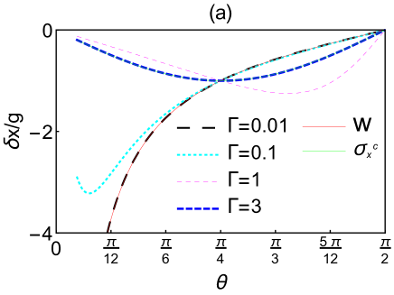
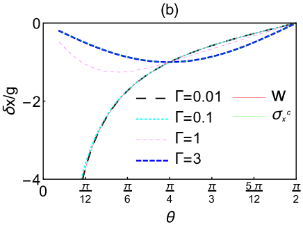
Figure 2: Weak-to-strong measurement transition, as characterized by position shift (see the Eq.(52)) of the coherent pointer state. The $\delta x_{coh}$ is shown as function of system postselected state parameter $\theta$ for different values of the coupling strengths $\Gamma$: (a) $r=3$ and (b) $r=0$. Here, we take $\varphi=\frac{\pi}{6}$.

Momentum shift. The momentum shift of the coherent pointer state also can be obtained by substituting the form of the state into Eq. (48). Its explicit expression reads as follows

$$\delta p_{coh} =\langle\Psi^{\prime\prime}|\hat{P}|\Psi^{\prime\prime}\rangle-\langle\beta|\hat{P}|\beta\rangle$$

$$=-\frac{1}{2\sigma\left(1-\cos\left(2\theta\right)\cos\left(2\Gamma r\sin\varphi\right)e^{-\frac{1}{2}\Gamma^{2}}\right)}$$

$$\times\{2iIm(\beta^{\ast})-i\sin\left(2\Gamma r\sin\varphi\right)\cos(2\theta)e^{-\frac{1}{2}\Gamma^{2}}\Gamma$$

$$\!\!-\!2iIm(\beta^{\ast})\cos(2\theta)\cos\left(2\Gamma r\sin\varphi\right)e^{-\frac{1}{2}\Gamma^{2}}\!\}\!+\!\frac{1}{2\sigma}2Im(\beta^{\ast}).$$ (55)

It is obvious from the above expression that the factor $e^{-\frac{1}{2}\Gamma^{2}}$ can be used to control the measurement regimes in the same way as the position shift. Similarly, we obtain

$$\left(\delta p\right)_{weak} =\lim_{\Gamma\rightarrow 0}\delta p_{coh}=0$$ (56)

and

$$\left(\delta p\right)_{st} =\lim_{\Gamma\rightarrow\infty}\delta p_{coh}=0,$$ (57)

respectively. These results well support our theoretical derivations given in Sec. II. Notice that in this scheme the weak value is real, whereas in general the momentum shift of the pointer in postselected weak measurement is proportional to the imaginary part of the weak value [see the Eq.(45)]. Thus, in our current case the momentum shift of the pointer for weak measurement vanishes. In Fig. 3, we show the the momentum shift [see Eq. (55)] as a function of parameter $\theta$.

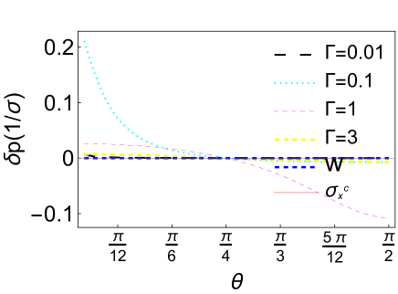
Figure 3: Momentum shift of the coherent pointer state after postselected von Neuamann measurement as function of system postselected state parameter $\theta$ for various coupling strengths $\Gamma$. Here we take $\varphi=\frac{\pi}{6}$ , $r=3$.

In Ref. (Pan et al., 2020), the authors have experimentally studied the weak-to-strong measurement transition problem in ${}^{40}Ca^{+}$ trapped ion system by considering a zero mean Gaussian as a pointer. The zero Gaussian profile corresponds to the ground state ($n=0$) of the coherent pointer state. Thus, our discussion in this section can be seen as an extension of the theoretical part of Ref. (Pan et al., 2020).

IV.2 The phase space function—– the Husimi-Kano Q function

In this subsection, in order to better visualize the weak-to-strong transition for coherent pointer states, we calculate the phase space distribution— $Q$ function. In quantum mechanics, Heisenberg’s uncertainty relations prevent the notion of a system being characterized by a point in phase space. However, since coherent states minimize the uncertainty product for two orthogonal quadrature operators and the two uncertainties are equal, we can write the phase space distribution of a quantum states by using the coherent state representation. Notice that the quadrature operators are dimensionless and scaled versions of the position and momentum operators. There are three main phase space quasi-probability distributions (Gerry and Knight, 2005), i.e. the Glauber-Sudarshan P-function, the Husimi-Kano Q function, and the Wigner function. Among them, the Q function is the expectation value of the density operator on a coherent state. As shown in (Tombesi and Pike, 1989) the interference effect in phase space can be described by considering the properties of Q function

$$Q_{\psi}(\alpha)=\frac{1}{\pi}|\langle\alpha|\psi\rangle|^{2}$$ (58)

for the state $|\psi\rangle$ under study. This expression may also be rewritten as

$$\langle\alpha|\psi\rangle=\sqrt{\pi Q_{\psi}(\alpha)}e^{i\phi_{\psi}(\alpha)}\,.$$ (59)

If $|\alpha\rangle$ and $|\psi\rangle$ denote two different quantum states, then their inner product $\langle\alpha|\psi\rangle$ is linked to the overlap in the phase space. In particular, $\pi Q_{\psi}(\alpha)$ denotes the overlap and $\phi_{\psi}(\alpha)$ is its phase. If we take $|\psi\rangle=|\Psi^{\prime\prime}\rangle$, its $Q$ function can be calculated as

$$Q_{\Psi^{\prime\prime}}(\alpha) =\frac{1}{\pi}|\langle\alpha|\Psi^{\prime\prime}\rangle|^{2}$$

$$=\frac{1}{\pi}\frac{1}{1-\cos\left(2\theta\right)\cos\left(2\Gamma r\sin\varphi\right)e^{-\frac{1}{2}\Gamma^{2}}}$$

$$\!\!\!\!\times\!\!\{\sin^{2}\left(\frac{\pi}{4}-\!\theta\right)e^{-|\alpha-\beta-\frac{\Gamma}{2}|^{2}}\text{\!\!\!}+\cos^{2}\left(\!\frac{\pi}{4}-\!\theta\right)e^{-|\alpha-\beta+\frac{\Gamma}{2}|^{2}}$$

$$-\cos 2\theta\cos\left(2\Gamma r\sin\varphi\right)e^{-\frac{1}{2}|\alpha-\beta-\frac{\Gamma}{2}|^{2}}e^{-\frac{1}{2}|\alpha-\beta+\frac{\Gamma}{2}|^{2}}\}.$$ (60)

The $Q$- function of our initial coherent pointer state $|\beta\rangle$ is given by

$$Q_{coh}(\alpha)=\frac{1}{\pi}|\langle\alpha|\beta\rangle|^{2}=\frac{1}{\pi}e^{-|\alpha-\beta|^{2}}.$$ (61)

By comparing the Eqs. (60) and (61), we can see that $Q_{\Psi^{\prime\prime}}(\alpha)$ contains three terms: the first and second terms represent the $Q-$functions of two different coherent states with amplitudes $|\beta+\frac{\Gamma}{2}|$ and $|\beta-\frac{\Gamma}{2}|$, respectively, whereas the third one describes their interference. The extra $\pm\frac{\Gamma}{2}$ in the exponential function part of the first and second terms of Eq.(60) [compare to Eq. (61)] are caused by the interaction between the measured system and the pointer. After the measurement, the wave-packet separates into sub-wave-packets corresponding to the two eigenvalues of the Pauli-$x$ operator. We also notice that in this expression the transition factor $e^{-\frac{1}{2}\Gamma^{2}}$ is still present. If we fix the coherent state parameter $\beta$, with the increasing of the coupling parameter $\Gamma$, the overlap gradually decreases and the third term vanishes. To describe the measurement transition phenomena in the phase-space, we show, in Fig. 4, the function $Q_{\Phi}(\alpha)$ function for different coupling strengths $\Gamma$. In panel (a) we see the $Q$- function of the coherent state $|\beta\rangle$, which is a Gaussian located at $\alpha_{r}=\sqrt{3}/2$ and $\alpha_{i}=1/2$. This Gaussian function is symmetric, the corresponding contour plot denotes the $1/e$ decay of the $Q_{coh}(\alpha)$-function. If the interaction is weak, there are two overlapping Gaussian wave-packets and thus interference effects appear, due to the third term in Eq.(60) [see the Fig. 4 (b)-(e)] . However, as it can be seen in Fig. 4(f), if the coupling between the system and pointer is strong enough, the initially overlapping two sub-wave-packets are fully separated, and the measurement transition from weak to strong measurement regimes occured. Here we take $\beta=\beta_{r}+i\beta_{i}=\sqrt{3}/2+0.5i$, though the $Q$-function of a coherent state is always a Gaussian fuction, independently on the value of the parameters $\beta_{r}$ and $\beta_{i}$. By comparing Fig.4(a) to Fig.4(e) and (f), we find that the radius of the circular contour plot is indeed independent of $\beta$. Since a coherent state corresponds to a displaced ground state of a harmonic oscillator, the fluctuations of the electric field operator in a coherent state are independent of the displacement $\beta$, i.e. fluctuations are only determined by the properties of the harmonic oscillator, and not by the displacement amplitude.

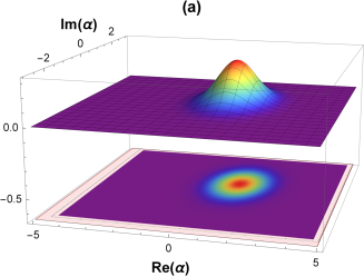
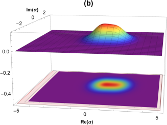
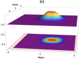
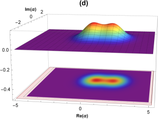
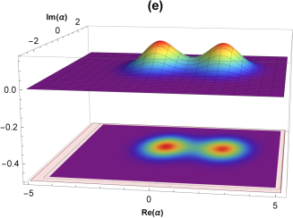
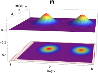
Figure 4: $Q_{\Phi}(\alpha)$ function (see the Eq. (60)) for different coupling strengths $\Gamma$ : (a) no interaction case ($\Gamma=0$); (b) $\Gamma=0.5$; (c) $\Gamma=1$; (d) $\Gamma=2$; (e) $\Gamma=3$; (f) $\Gamma=5$. Here, we take $r=1$, $\varphi=\frac{\pi}{6}$, and $\theta=0.01$.

V A possible experimental realization

In this Section, we put forward a possible implementation of our measurement scheme in a trapped-ion system. As shown in previous studies , [8], trapped ions subject to laser cooling represent an excellent platform for quantum state preparation and manipulation (Cirac et al., 1993a) since they are characterized by a decoherence time much longer than the typical times required to perform quantum measurements. Furthermore, the (quantum) motion state of trapped ions can be fully characterized by quantum tomographic measurements (Wallentowitz and Vogel, 1995; Leibfried et al., 1996). Up to date, a variety of schemes have been proposed and experimentally observed for the preparation of nonclassical motional states of a trapped ion (Meekhof et al., 1996; Zeng and Lin, 1993; Kienzler et al., 2015; Mccormick et al., 2019), such as Fock (Cirac et al., 1993b), coherent (Hume et al., 2011; Munro et al., 2000; Raffa et al., 2012; Alonso et al., 2016), squeezed (Zeng and Lin, 1995; Cirac et al., 1993a; Drechsler et al., 2020), Schrodinger cat (de Matos Filho and Vogel, 1996; Poyatos et al., 1996; Gerry, 1997; Haroche and J.-M.Raymond, 2006; Wineland, 2013), pair coherent (Gou et al., 1996a), and pair cat (Gou et al., 1996b) states. In order to implement our scheme, we consider an ion trapped in a harmonic potential with frequency $\nu$, and driven by two laser beams interacting resonantly with the system, tuned to the lower (red) and upper (blue) vibrational sidebands, respectively. By taking the Lamb-Dicke regime (Javanainen, 1981) into account, the total system Hamiltonian in the interaction picture is given by (Zheng, 1998; Wallentowitz and Vogel, 1995)

$$H =\eta\Omega\left(\hat{\sigma}_{x}\sin\phi_{+}+\hat{\sigma}_{y}\cos\phi_{+}\right)$$

$$\otimes\left(\sigma\sin\phi_{-}\hat{P}-\frac{\hbar}{2\sigma}\cos\phi_{-}\hat{X}\right),$$ (62)

where $\eta$ is the Lamb-Dcike parameter, $\Omega$ is the Rabi frequency, and $\phi_{\pm}=\frac{1}{2}\left(\phi_{red}\pm\phi_{blue}\right)$ are phases depending on the lower and upper sideband lasers phases $\phi_{red}$ and $\phi_{blue}$. Here, $\hat{X}=\sigma\left(\hat{a}+\hat{a}^{\dagger}\right)$ and $\hat{P}=\frac{i}{2\sigma}\left(\hat{a}^{\dagger}-\hat{a}\right)$ are the position and momentum operators of the vibrational degree of freedom of the ion, and $\sigma=\sqrt{1/2\nu m}$ characterizes the size of the motional state, which itself depends on the mass $m$ and on the vibrational $\nu$ of the ion. Another important point is that here the ion is considered as a two level system. In the above Hamiltonian, the $\hat{\sigma}_{x}$ and $\hat{\sigma}_{y}$ are the Pauli-$x$ and -$y$ operatorsm which can be written in terms of ion’s ground ($|\downarrow\rangle$) and optically excited ($|\uparrow\rangle$) states as $\hat{\sigma}_{x}=|\uparrow\rangle\langle\downarrow|+|\downarrow\rangle\langle\uparrow|$ and $\hat{\sigma}_{y}=i\left(|\uparrow\rangle\langle\downarrow|-|\downarrow\rangle\langle\uparrow|\right)$, respectively. The Lamb-Dcike parameter $\eta$ is related to the wave vector $k$, and is given by$\eta=k/\sqrt{2\nu m}$. In the derivation of the above Hamiltonian we have assumed $\eta\ll 1$.

If we take the external and internal parts of the two level trapped ion as the pointer and measured system, respectively, Eq. (62) describes the typical von Neumann type measurement by adjusting some of the parameters. In general, the system observable $\hat{A}$ satisfies $\hat{A}^{2}=\hat{A}$ or $\hat{A}^{2}=\hat{I}$, and the $\hat{A}^{2}=\hat{I}$ case is very usual in measurement problems. If we set $\phi_{-}=\frac{\pi}{2}$ , $\phi_{+}=\frac{\pi}{2}$ or $0$, the above interaction Hamiltonian takes the form

$$H=g\hat{\sigma}_{x}\otimes\hat{P},$$ (63)

or

$$H=g\hat{\sigma}_{y}\otimes\hat{P},$$ (64)

respectively, with $g=\eta\sigma\Omega$. These correspond to the von Nuemann type measurement Hamiltonians introduced in Sec. II. In a recent study (Pan et al., 2020), the authors have investigated the weak-to-strong measurement transition problem by taking a zero mean Gaussian state as pointer in ${}^{40}Ca^{+}$ trapped ion system. Since state preparation in trapped ion system is very realiable, and the generated states are stable and mantain coherence over a long time, we anticipate that our general approach to weak-to-strong measurement transition may be implemented by using the Hamiltonians in Eq. (63) or Eq.(64) using Fock (José and Mizrahi, 2000; Um et al., 2016; Wolf et al., 2019; Simón et al., 2020), SPACS (Kienzler et al., 2015) and Schodinger cat pointer states (Kienzler et al., 2016).

VI Conclusion and remarks

In conclusion, we have given a general expressions of the position and momentum shifts which holds for any infinite-dimensional pointer states and any value of coupling strengths between the measured system and the pointer. At first, we have derived the general formula of the position shift corresponding to postselected weak measurements [see Eq. (29)], and have verified that it agrees with previous results. We have also proved that by adjusting the coupling strength parameter $\Gamma$, we can link the weak value and the conditional expectation value of system observable obtained by the shifts of the pointer in weak and strong measurement regimes, respectively. As a typical example of our general approach, we have illustrated the weak-to-strong measurement transition for a coherent pointer state, also analyzing the phenomenon in the phase space by using the $Q$- function. Finally, we have discussed a possible experimental realization of our weak-to-strong measurement transition scheme in trapped ion system.