Numerical sign problem and the tempered Lefschetz thimble method

Abstract

The numerical sign problem is a major obstacle to the quantitative understanding of many important physical systems with first-principles calculations. Typical examples for such systems include finite-density QCD, strongly-correlated electron systems and frustrated spin systems, as well as the real-time dynamics of quantum systems. In this talk, we argue that the tempered Lefschetz thimble method (TLTM) [M. Fukuma and N. Umeda, arXiv:1703.00861] and its extension, the worldvolume tempered Lefschetz thimble method (WV-TLTM) [M. Fukuma and N. Matsumoto, arXiv:2012.08468], may be a reliable and versatile solution to the sign problem. We demonstrate the effectiveness of the algorithm by exemplifying a successful application of WV-TLTM to the Stephanov model, which is an important toy model of finite-density QCD. We also discuss the computational scaling of WV-TLTM.

1 Introduction

The numerical sign problem has prevented us from the quantitative understanding of many important physical systems with first-principles calculations. Typical examples for such systems include finite-density QCD, strongly-correlated electron systems and frustrated spin systems, as well as the real-time dynamics of quantum systems.

The main aim of this talk is to argue that the tempered Lefschetz thimble method (TLTM) [11] and its extension, the worldvolume tempered Lefschetz thimble method (WV-TLTM) [15], may be a reliable and versatile solution to the sign problem. The (WV-)TLTM actually has been confirmed to work for toy models of some of the systems listed above. In this talk, we pick up the Stephanov model, to which the WV-TLTM is applied. This matrix model has played a particularly important role in attempts to establish a first-principles calculation method for finite-density QCD, because it well approximates the qualitative behavior of finite-density QCD at large matrix sizes, and because it has a serious sign problem which had not been solved by other methods than the (WV-)TLTM. We also discuss the computational scaling of WV-TLTM.

2 Sign problem

2.1 What is the sign problem?

Our aim is to numerically estimate the expectation value defined in a path-integral form:

$$\langle\mathcal{O}(x)\rangle\equiv\frac{\int dx\,e^{-S(x)}\,\mathcal{O}(x)}{\int dx\,e^{-S(x)}}.$$ (1)

Here, $x=(x^{i})\in{\mathbb{R}}$ is a dynamical variable of $N$ degrees of freedom (DOF), $S(x)$ the action, and $\mathcal{O}(x)$ a physical observable of interest.

When $S(x)$ is real-valued, one can regard $p_{\rm eq}(x)\equiv e^{-S(x)}/\int dx\,e^{-S(x)}$ as a probability distribution, and can estimate $\langle\mathcal{O}(x)\rangle$ with a sample average as

$$\langle\mathcal{O}(x)\rangle\approx\frac{1}{N_{\rm conf}}\,\sum_{k=1}^{N_{\rm conf}}\mathcal{O}(x^{(k)}).$$ (2)

Here, $\{x^{(k)}\}$ is a sample (a set of configurations) of size $N_{\rm conf}$, that is generated as a suitable Markov chain with the equilibrium distribution $p_{\rm eq}(x)$.

The above prescription is no longer applicable when the action has an imaginary part as $S(x)=S_{R}(x)+iS_{I}(x)\in{\mathbb{C}}^{N}$. A naive way to handle this is the so-called reweighting method, where we treat $e^{-S_{R}(x)}/\int dx\,e^{-S_{R}(x)}$ as a new weight and rewrite the expression (1) as a ratio of reweighted averages:

$$\langle\mathcal{O}(x)\rangle=\frac{\langle e^{-iS_{I}(x)}\,\mathcal{O}(x)\rangle_{\rm rewt}}{\langle e^{-iS_{I}(x)}\,\rangle_{\rm rewt}}\quad\Bigl{(}\langle f(x)\rangle_{\rm rewt}\equiv\frac{\int dx\,e^{-S_{R}(x)}\,f(x)}{\int dx\,e^{-S_{R}(x)}}\Bigr{)}.$$ (3)

However, when the DOF, $N$, is very large, the reweighted averages can become vanishingly small of $e^{-O(N)}$, even though the operator itself is $O(1)$. This should not be a problem if we can estimate both the numerator and the denominator precisely. However, in the numerical computation, they are estimated separately with statistical errors:

$$\langle\mathcal{O}(x)\rangle\equiv\frac{\langle e^{-iS_{I}(x)}\mathcal{O}(x)\rangle_{\rm rewt}}{\langle e^{-iS_{I}(x)}\rangle_{\rm rewt}}\approx\frac{e^{-O(N)}\pm O(1/\sqrt{N_{\rm conf}})}{e^{-O(N)}\pm O(1/\sqrt{N_{\rm conf}})}.$$ (4)

Thus, in order for the statistical errors to be smaller than the mean values, the sample size must be exponentially large with respect to DOF, namely, $N_{\rm conf}\gtrsim e^{O(N)}$. The need of this unrealistically large numerical cost is called the sign problem.

2.2 Various approaches proposed so far

We list some of the approaches proposed so far, which are intended to solve the sign problem.

class 1: no use of reweighting

A typical algorithm in this class is the complex Langevin method [1, 2, 3, 4, 5, 6], where the complex Boltzmann weight is rewritten to a positive probability distribution over a complex space ${\mathbb{C}}^{N}$. Although its numerical cost is low $[\sim O(N)]$, it often exhibits a wrong convergence (gives incorrect estimates with small statistical errors) at parameter values of physical importance.

class 2: deforming the integration surface

A typical algorithm is the Lefschetz thimble method [7, 8, 9, 10, 11, 12, 13, 14, 15, 16], where the integration surface $\Sigma_{0}={\mathbb{R}}^{N}$ is continuously deformed to a new surface $\Sigma_{t}\subset{\mathbb{C}}^{N}$. The flow time $t$ is taken sufficiently large so that $\Sigma_{t}$ is close to a union of Lefschetz thimble, $\bigcup_{\sigma}\mathcal{J}_{\sigma}$, on each of which ${\rm Im}\,S(z)$ $(z\in\mathcal{J}_{\sigma})$ is constant.

Generic Lefschetz thimble method has been shown to suffer from an ergodicity problem for physically important parameter regions of a model [19], where multiple thimbles become relevant that are separated by infinitely high potential barriers. This problem was resolved by tempering the system with the flow time [11]. This tempered Lefschetz thimble method (TLTM) solves both the sign problem (serious at small flow times) and the ergodicity problem (serious at large flow times) simultaneously. The disadvantage is its high numerical cost of $O(N^{3-4})$. Recently, this numerical cost has been substantially reduced [expected to be $O(N^{\sim 2.25})$] with a new method, the worldvolume tempered Lefschetz thimble method (WV-TLTM), which is based on the idea to perform the Hybrid Monte Carlo on a continuous accumulation of deformed integration surfaces (the worldvolume) [15]. The algorithm (WV-)TLTM is the main subject in this talk.

class 3: no use of MC in the first place

A typical algorithm in this class is the tensor network method (especially the tensor renormalization group method [21]). This is good at calculating the free energy in the thermodynamic limit, but not so much efficient to calculate correlation functions at large distances. We expect this method to play a complementary role to methods based on Markov chain Monte Carlo.

3 Lefschetz thimble method

We complexify the dynamical variable $x=(x^{i})\in{\mathbb{R}}^{N}$ to $z=(z^{i}=x^{i}+iy^{i})\in{\mathbb{C}}^{N}$. We set an assumption (which holds for most cases) that $e^{-S(z)}$ and $e^{-S(z)}\mathcal{O}(z)$ are entire functions over ${\mathbb{C}}^{N}$. Then, Cauchy’s theorem ensures that the integrals do not change their values under continuous deformation of the integration surface: $\Sigma_{0}={\mathbb{R}}^{N}\to\Sigma\,(\subset{\mathbb{C}}^{N})$, where the boundary at $|x|\to\infty$ is fixed so that the convergence of integration holds under the deformation:

$$\langle\mathcal{O}(x)\rangle=\frac{\int_{\Sigma_{0}}dx\,e^{-S(x)}\,\mathcal{O}(x)}{\int_{\Sigma_{0}}dx\,e^{-S(x)}}=\frac{\int_{\Sigma}dz\,e^{-S(z)}\,\mathcal{O}(z)}{\int_{\Sigma}dz\,e^{-S(z)}}.$$ (5)

Thus, even when the sign problem is severe on the original surface $\Sigma_{0}$, it will be significantly reduced if ${\rm Im}\,S(z)$ is almost constant on the new surface $\Sigma$.

The prescription for the deformation is given by the anti-holomorphic gradient flow:

$$\dot{z}_{t}=\overline{\partial S(z_{t})}\quad\mbox{with}\quad z_{t=0}=x.$$ (6)

The most important property of this flow equation is the following inequality:

$$[S(z_{t})]^{\cdot}=\partial S(z_{t})\cdot\dot{z}_{t}=|\partial S(z_{t})|^{2}\geq 0,$$ (7)

from which we find that

(i)  ${\rm Re}\,S(z_{t})$ always increases along the flow except at critical points,

(ii) ${\rm Im}\,S(z_{t})$ is constant along the flow.

The Lefschetz thimble $\mathcal{J}$ associated with a critical point $\zeta$ is defined by a set of orbits starting at $\zeta$. From this construction and property (ii), we easily see that ${\rm Im}\,S(z)$ is constant on $\mathcal{J}$ [i.e., ${\rm Im}\,S(z)={\rm Im}\,S(\zeta)~{}(z\in\mathcal{J})$]. Denoting the solution of Eq. (6) by $z_{t}(x)$ and assuming that $\Sigma_{t}\equiv\{z_{t}(x)|\,x\in{\mathbb{R}}^{N}\}$ approaches a single Lefschetz thimble $\mathcal{J}$, we expect that the sign problem disappears on $\Sigma_{t}$ if we choose a sufficiently large $t$.

Let us see how the sign problem disappears as flow time $t$ increases. The integrals on a deformed surface $\Sigma_{t}$ can be rewritten as

$$\langle\mathcal{O}(x)\rangle=\frac{\langle e^{i\phi(z)}\mathcal{O}(z)\rangle_{\Sigma_{t}}}{\langle e^{i\phi(z)}\rangle_{\Sigma_{t}}},$$ (8)

where

$$\langle f(z)\rangle_{\Sigma_{t}}\equiv\frac{\int_{\Sigma_{t}}|dz|\,e^{-{\rm Re}\,S(z)}f(z)}{\int_{\Sigma_{t}}|dz|\,e^{-{\rm Re}\,S(z)}},\quad e^{i\phi(z)}\equiv e^{-i{\rm Im}\,S(z)}\,\frac{dz}{|dz|}.$$ (9)

As can be easily checked for a Gaussian case, the integrals take the form $O(e^{-e^{-\lambda t}O(N)})$, where $\lambda$ is a typical singular value of $\partial_{i}\partial_{j}S(\zeta)$. Thus, the numerical estimate now becomes

$$\langle\mathcal{O}(x)\rangle\approx\frac{O(e^{-e^{-\lambda t}O(N)})\pm O(1/\sqrt{N_{\rm conf}})}{O(e^{-e^{-\lambda t}O(N)})\pm O(1/\sqrt{N_{\rm conf}})},$$ (10)

from which we see that the main parts become $O(1)$ when the flow time $t$ satisfies a relation $e^{-\lambda t}O(N)=O(1)$. We thus see that the sign problem disappears at flow times $t\gtrsim T=O(\ln N)$.

4 Tempered Lefschetz thimble method (TLTM)

4.1 Ergodicity problem in the original Lefschetz thimble method

So far, so good; when a single Lefschetz thimble is relevant to estimation, one can resolve the sign problem simply by taking a sufficiently large flow time. However, this nice story no longer holds true when multiple thimbles are involved in estimation, because there comes up another problem (ergodicity problem) as the flow time increases.

Figure 1 describes the case $e^{-S(x)}=e^{-\beta x^{2}/2}\,(x-i)^{\beta}$ $(\beta\gg 1)$. In addition to two critical points $\zeta_{\pm}=\pm\sqrt{3}/2+(1/2)\,i$ and the associated Lefschetz thimbles $\mathcal{J}_{\pm}$, here is the zero of $e^{-S(z)}$ at $z=i$. We see that the integration surface $\Sigma_{T}$ is separated into two parts by an infinitely high potential barrier at the zero. It is thus very hard for two configurations on different parts to communicate in stochastic processes, which means that it takes a very long computation time for the system to reach equilibrium.

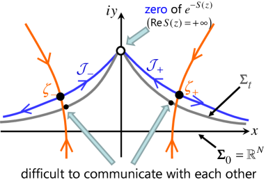
Figure 1: Ergodicity problem.

4.2 Basic algorithm of TLTM

The tempered Lefschetz thimble method [11] was invented to overcome this problem by implementing the tempering algorithm [23, 24, 25, 26] to the thimble method, where the flow time is used as a tempering parameter (see Fig. 2). The basic algorithm goes as follows:

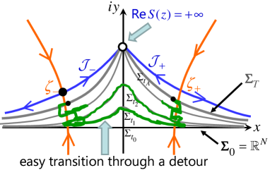
Figure 2: Tempered Lefschetz thimble method (TLTM).

Step 0.  We fix the target flow time $T$ so that the sign problem is not serious for a sample on $\Sigma_{T}$ except for the ergodicity problem. This is judged by looking at the average phase factor $|\langle e^{i\phi(z)}\rangle_{\Sigma_{T}}|$.

Step 1.  We introduce replicas in between the initial integration surface $\Sigma_{0}={\mathbb{R}}^{N}$ and the target deformed surface $\Sigma_{T}$ as $\{\Sigma_{t_{0}=0},\Sigma_{t_{1}},\ldots,\Sigma_{t_{A}=T}\}$.

Step 2.  We set up a Markov chain for the extended configuration space $\{(x,t_{\alpha})|\,x\in{\mathbb{R}}^{N},\,\alpha=0,1,\ldots,A\}$.

Step 3.  After equilibration, we estimate observables with a sample on $\Sigma_{T}$.

This tempering method prompts the equilibration on $\Sigma_{T}$ because two configurations on different connected components now can communicate easily by passing through a detour. Thus, the TLTM solves both the sign and ergodicity problems simultaneously.

4.3 Comment on transitions between adjacent replicas

We here comment that one can expect a significant acceptance rate for transitions between adjacent replicas [13]. To see this, let us use the initial configurations $x\in{\mathbb{R}}^{N}$ as common coordinates for different replicas. When we employ the simulated tempering [23] for a tempering method as in the previous subsection, a configuration $(x,t_{\alpha})$ moves to $(x,t_{\alpha\pm 1})$ (after it explores on $\Sigma_{t_{\alpha}}$), keeping the $x$-coordinate values the same. Since the probability distribution on every replica has peaks at the same points $x_{\sigma}$, where $x_{\sigma}$ flows to a critical point $z_{\sigma}$, we can expect a significant overlap between distributions on two adjacent replicas.

4.4 Computational cost for the original TLTM

An obvious advantage of the original TLTM is its versatility; the method can be applied to any system once it is formulated in a path-integral form with continuous variables, resolving the sign and ergodicity problems simultaneously. A disadvantage is its high numerical cost. It is expected to be $O(N^{3-4})$ due to (a) the increase of the necessary number of replicas [probably as $O(N^{0-1})$] and (b) the need to compute the Jacobian matrix of the flow, $J(x)\equiv(\partial z^{i}_{t}(x)/\partial x^{a})$, every time we move configurations between adjacent replicas [$O(N^{3})$]. The worldvolume TLTM [15] was introduced to significantly reduce the computational cost.

5 Worldvolume tempered Lefschetz thimble method (WV-TLTM)

5.1 Basic idea of the Worldvolume TLTM

Instead of introducing a finite set of replicas (a finite set of integrations surfaces), we consider in the WV-TLTM a HMC algorithm on a continuous accumulation of deformed integration surfaces,

$$\mathcal{R}\equiv\bigcup_{0\leq t\leq T}\Sigma_{t}=\bigl{\{}z_{t}(x)\big{|}\,t\in[0,T],~{}x\in{\mathbb{R}}^{N}\bigr{\}}.$$ (11)

We call $\mathcal{R}$ the worldvolume because this is an orbit of integration surface in the “target space” ${\mathbb{C}}^{N}={\mathbb{R}}^{2N}$ (see Fig. 3).

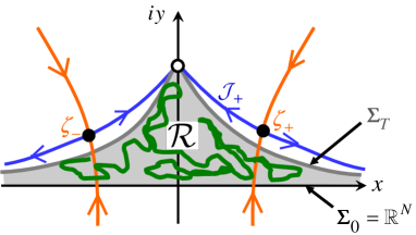
Figure 3: Worldvolume $\mathcal{R}$ of WV-TLTM.

Keeping the original virtues intact (solving the sign and ergodicity problems simultaneously), the new algorithm significantly reduces the computational cost. In fact, we no longer need to introduce replicas explicitly or to calculate the Jacobian matrix in every molecular dynamics process, and we can move configurations largely due to the use of HMC algorithm.

The key idea behind the algorithm is again Cauchy’s theorem. We start from the expression (5):

$$\langle\mathcal{O}(x)\rangle=\frac{\int_{\Sigma_{0}}dx\,e^{-S(x)}\,\mathcal{O}(x)}{\int_{\Sigma_{0}}dx\,e^{-S(x)}}=\frac{\int_{\Sigma_{t}}dz_{t}\,e^{-S(z_{t})}\,\mathcal{O}(z_{t})}{\int_{\Sigma_{t}}dz_{t}\,e^{-S(z_{t})}}.$$ (12)

Cauchy’s theorem ensures that both the numerator and the denominator do not depend on $t$, so that we can average over $t$ with an arbitrary weight $e^{-W(t)}$, leading to an integration over $\mathcal{R}$:

$$\langle\mathcal{O}(x)\rangle=\frac{\int_{0}^{T}dt\,e^{-W(t)}\int_{\Sigma_{t}}dz_{t}\,e^{-S(z_{t})}\mathcal{O}(z_{t})}{\int_{0}^{T}dt\,e^{-W(t)}\int_{\Sigma_{t}}dz_{t}\,e^{-S(z_{t})}}=\frac{\int_{\mathcal{R}}dt\,dz_{t}\,e^{-W(t)-S(z_{t})}\mathcal{O}(z_{t})}{\int_{\mathcal{R}}dt\,dz_{t}\,e^{-W(t)-S(z_{t})}}.$$ (13)

5.2 Algorithm

An explicit implementation can go in two ways, as described in the original paper [15]. One is the target-space picture, in which the HMC is performed on the worldvolume $\mathcal{R}$ that is treated as a submanifold in the target space ${\mathbb{C}}^{N}$. The other is the parameter-space picture, in which the HMC is performed on the parameter space $\{(x,t)\}$.

In the target-space picture, we first parametrize the induced metric on $\mathcal{R}$ with the ADM decomposition [28]:

$$ds^{2}=\alpha^{2}\,dt^{2}+\gamma_{ab}\,(dx^{a}+\beta^{a}\,dt)\,(dx^{b}+\beta^{b}\,dt).$$ (14)

Here, the functions $\alpha$ and $\beta^{a}$ are called the lapse and the shifts, respectively, and $\gamma_{ab}$ is the induced metric on $\Sigma_{t}$. The invariant volume element on $\mathcal{R}$ is then given by

$$Dz=\alpha\,dt\,|dz_{t}(x)|=\alpha\,|\det J|\,dt\,dx\quad\bigl{(}|\det J|=\sqrt{\det\gamma}\bigr{)},$$ (15)

and the expectation value can be rewritten to a ratio of reweighted averages on $\mathcal{R}$:

$$\langle\mathcal{O}(x)\rangle=\frac{\int_{\mathcal{R}}Dz\,e^{-V(z)}\,A(z)\,\mathcal{O}(z)}{\int_{\mathcal{R}}Dz\,e^{-V(z)}\,A(z)}=\frac{\langle A(z)\,\mathcal{O}(z)\rangle_{\mathcal{R}}}{\langle A(z)\rangle_{\mathcal{R}}}.$$ (16)

Here, the reweighted average of a function $f(z)$ is defined by

$$\langle f(z)\rangle_{\mathcal{R}}\equiv\frac{\int_{\mathcal{R}}Dz\,e^{-V(z)}\,f(z)}{\int_{\mathcal{R}}Dz\,e^{-V(z)}}$$ (17)

with $V(z)\equiv{\rm Re}\,S(z)+W(t(z))$, and the associated reweighting factor takes the form

$$A(z)\equiv\frac{dt\,dz_{t}}{Dz}\,e^{-i{\rm Im}\,S(z)}=\alpha^{-1}(z)\,\frac{\det J}{|\det J|}\,e^{-i{\rm Im}\,S(z)}.$$ (18)

The reweighted average can be estimated with the RATTLE algorithm [29, 30], where molecular dynamics is performed on $\mathcal{R}$ which is treated as a submanifold of ${\mathbb{C}}^{N}$ [15]. The algorithm takes the following form (see Fig. 4):

$$\pi_{1/2} =\pi-\Delta s\,\bar{\partial}V(z)-\lambda^{a}F_{a}(z),$$ (19)

$$z^{\prime} =z+\Delta s\,\pi_{1/2},$$ (20)

$$\pi^{\prime} =z-\Delta s\,\bar{\partial}V(z^{\prime})-\lambda^{\prime a}F_{a}(z^{\prime}).$$ (21)

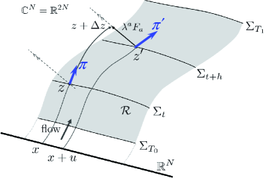
Figure 4: RATTLE on the worldvolume $\mathcal{R}$ [15].

Here, $F_{a}(z)\equiv iJ_{a}(z)$ $(a=1,\ldots,N)$ with $J_{a}\equiv(J^{i}_{a}=\partial z^{i}_{t}(x)/\partial x^{a})$ form a basis of the normal space $N_{z}\Sigma_{t}$ at $z\in\Sigma_{t}\,(\subset\mathcal{R})$. The Lagrange multipliers $\lambda^{a}$ and $\lambda^{\prime a}$ are determined using $E_{0}(z)\equiv\overline{\partial S(z)}$ such that

$$\bullet ~{}~{}z^{\prime}\in\mathcal{R}~{}~{}~{}\mbox{and}~{}~{}~{}\lambda^{a}F_{a}(z)\perp E_{0}(z),$$ (22)

$$\bullet ~{}~{}\pi^{\prime}\in T_{z^{\prime}}\mathcal{R}~{}~{}~{}\mbox{and}~{}~{}~{}\lambda^{\prime a}F_{a}(z^{\prime})\perp E_{0}(z^{\prime}).$$ (23)

The second equation in each line ensures that $\lambda^{a}F_{a}(z)$ actually belongs to $N_{z}\mathcal{R}\,(\subset N_{z}\Sigma_{t})$. The statistical analysis method for WV-TLTM (or more generally, for WV-HMC that is the HMC algorithm on a foliated manifold) is established in Ref. [16].

5.3 Various models to which (WV-)TLTM is applied

The (WV-)TLTM has been successfully applied to various models, including
$\bullet$  $(0+1)$-dimensional massive Thirring model [11]
$\bullet$  two-dimensional Hubbard model [13, 14]
$\bullet$  Stephanov model (a chiral random matrix model as a toy model of finite density QCD) [15]
$\bullet$  antiferromagnetic Ising model on the triangular lattice [33].
Correct results have always been obtained when they can be compared with analytic results, although the system sizes are yet small.

In the next section, we discuss the application of WV-TLTM to the Stephanov model.

6 Application to the Stephanov model

6.1 Stephanov model

The finite density QCD is given by the following partition function after $N_{f}$ quark fields (assumed to have the same mass) are integrated out:

$$Z_{\rm QCD} ={\rm tr}\,e^{-\beta(H-\mu N)}$$

$$=\int[dA_{\mu}]\,e^{(1/2g_{0}^{2})\,\int d^{4}x\,{\rm tr}\,F_{\mu\nu}^{2}}\,{\rm Det}\,{}^{N_{f}}\left(\begin{array}[]{cc}m&\sigma_{\mu}(\partial_{\mu}+A_{\mu})+\mu\\ \sigma^{\dagger}(\partial_{\mu}+A_{\mu})+\mu&m\end{array}\right).$$ (26)

The Stephanov model [34, 35] takes the following form at temperature $T=0$:

$$Z_{\rm Steph}=\int d^{2}W\,e^{-n\,{\rm tr}\,W^{\dagger}W}\,\det{}^{N_{f}}\left(\begin{array}[]{cc}m&iW+\mu\\ iW^{\dagger}+\mu&m\end{array}\right),$$ (29)

where the $n\times n$ complex matrix $W=(W_{ij})=(X_{ij}+iY_{ij})$ represents quantum-field degrees of freedom (including space-time dependences). This model plays a particularly important role because (a) it well approximates the qualitative behavior of finite-density QCD at large matrix sizes and (b) it has a serious sign problem which can hardly be solved by the complex Langevin method due to a wrong convergence [36].

Figures 5 and 6 show the results for the chiral condensate $\langle\bar{\psi}\psi\rangle$ and the number density $\langle\psi^{\dagger}\psi\rangle$ at $n=10$, $m=0.004$ and $N_{f}=1$ obtained with the WV-TLTM, where the sample size is $N_{\rm conf}=4,000-17,000$ (varying on $\mu$). We see that they agree with the exact results within statistical errors. For comparison, we also plot the results obtained with the naive reweighting method (showing large deviations from the exact values due to the sign problem) and also with the complex Langevin method (exhibiting a serious wrong convergence). The sample size is $N_{\rm conf}=10^{4}$ for both the reweighting and the complex Langevin.

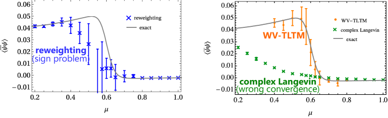
Figure 5: Chiral condensate $\langle\bar{\psi}\psi\rangle\equiv(1/2n)(\partial/\partial m)\ln Z_{\rm Steph}$ [15].

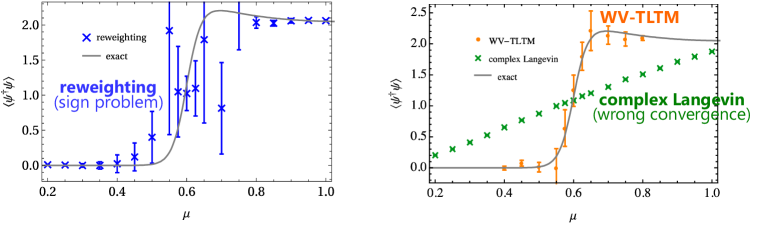
Figure 6: Number density $\langle\psi^{\dagger}\psi\rangle\equiv(1/2n)(\partial/\partial\mu)\ln Z_{\rm Steph}$ [15].

6.2 Computational scaling

In the RATTLE algorithm, we need to make an inversion of the linear problem, $Jv=b$ ($J$: the Jacobian matrix). The total numerical cost of WV-TLTM depends on which solver is used.

When a direct method (e.g., LU decomposition) is used, the computational cost is expected to be $O(N^{3})$. In this case, the Jacobian matrix $J=(J_{t}(x))$ is explicitly computed by numerically integrating the differential equation $\dot{J_{t}}=\overline{\partial^{2}S(z_{t})\,J_{t}}$ together with Eq. (6), whose cost is also $O(N^{3})$. Figure 7 shows the real computation time for generating a single configuration, performed on a supercomputer (Yukawa-21) at Yukawa Institute, Kyoto University. We clearly see that it scales as expected, and smaller than $O(N^{3-4})$ expected for the original TLTM. We also see that the aid of GPU is quite effective.

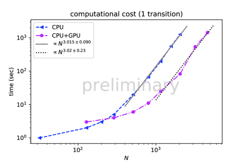
Figure 7: Computation time to generate a configuration with a direct method in the linear inversion.

The computational cost can be further reduced if we adopt an iterative method (such as BiCGStab) as in Ref. [32]. The numerical cost is then expected to be $O(N^{2})$ if the Krylov subspace iteration converges quickly. This factor will be multiplied by $O(N^{1/4})$ if we reduce the step size of molecular dynamics so that the acceptance rate of the final Metropolis test is independent of $N$.

7 Summary and outlook

We have reported that the tempered Lefschetz thimble method and its worldvolume extension, (WV-)TLTM, has a potential to be a reliable and versatile solution to the sign problem, because the algorithm solves the sign and ergodicity problems simultaneously and can be applied to any system in principle if it is formulated in a path-integral form with continuous variables. The (WV-)TLTM has been successfully applied to various models (yet only to toy models with small DOF at this stage), which include important toy models such as the Stephanov model (for finite density QCD), the 1D/2D Hubbard model (for strongly correlated electron systems), and the antiferromagnetic Ising model on the triangular lattice (for frustrated classical/quantum spin systems).

We are now porting the code of WV-TLTM such that it can run on a large-scale supercomputer, which we expect to be completed soon. In parallel with this, it should be important to keep improving the algorithm itself so that the estimation can be made more efficiently for large-scale systems. It would be also interesting to combine various algorithms that have been proposed as solutions to the sign problem. An interesting candidate we have in mind as a partner of (WV-)TLTM is the tensor renormalization group method, which is actually complementary to Monte Carlo method in many aspects. A particularly important subject in the near future will be to establish a Monte Carlo algorithm for the calculation of time-dependent systems. This will open a way to the quantitative understanding of nonequilibrium processes, such as those happening in heavy ion collision experiments and in the very early universe.

A study along these lines is in progress, and we hope we can report some of the achievements in the next Corfu conference.

References

- [1] G. Parisi, “On complex probabilities,” Phys. Lett. 131B, 393 (1983).
- [2] J. R. Klauder, “Stochastic quantization,” Acta Phys. Austriaca Suppl. 25, 251-281 (1983)
- [3] J. R. Klauder, “Coherent state Langevin equations for canonical quantum systems with applications to the quantized Hall effect,” Phys. Rev. A 29, 2036-2047 (1984)
- [4] G. Aarts, F. A. James, E. Seiler and I. O. Stamatescu, “Complex Langevin: Etiology and diagnostics of its main problem,” Eur. Phys. J. C 71, 1756 (2011) [arXiv:1101.3270 [hep-lat]].
- [5] G. Aarts, L. Bongiovanni, E. Seiler, D. Sexty and I. O. Stamatescu, “Controlling complex Langevin dynamics at finite density,” Eur. Phys. J. A 49, 89 (2013) [arXiv:1303.6425 [hep-lat]].
- [6] K. Nagata, J. Nishimura and S. Shimasaki, “Argument for justification of the complex Langevin method and the condition for correct convergence,” Phys. Rev. D 94, no. 11, 114515 (2016) [arXiv:1606.07627 [hep-lat]].
- [7] E. Witten, “Analytic Continuation Of Chern-Simons Theory,” AMS/IP Stud. Adv. Math. 50, 347-446 (2011) [arXiv:1001.2933 [hep-th]].
- [8] M. Cristoforetti, F. Di Renzo and L. Scorzato, “New approach to the sign problem in quantum field theories: High density QCD on a Lefschetz thimble,” Phys. Rev. D 86, 074506 (2012) [arXiv:1205.3996 [hep-lat]].
- [9] H. Fujii, D. Honda, M. Kato, Y. Kikukawa, S. Komatsu and T. Sano, “Hybrid Monte Carlo on Lefschetz thimbles - A study of the residual sign problem,” JHEP 1310, 147 (2013) [arXiv:1309.4371 [hep-lat]].
- [10] A. Alexandru, G. Başar, P. F. Bedaque, G. W. Ridgway and N. C. Warrington, “Sign problem and Monte Carlo calculations beyond Lefschetz thimbles,” JHEP 1605, 053 (2016) [arXiv:1512.08764 [hep-lat]].
- [11] M. Fukuma and N. Umeda, “Parallel tempering algorithm for integration over Lefschetz thimbles,” PTEP 2017, no. 7, 073B01 (2017) [arXiv:1703.00861 [hep-lat]].
- [12] A. Alexandru, G. Başar, P. F. Bedaque and N. C. Warrington, “Tempered transitions between thimbles,” Phys. Rev. D 96, no.3, 034513 (2017) [arXiv:1703.02414 [hep-lat]].
- [13] M. Fukuma, N. Matsumoto and N. Umeda, “Applying the tempered Lefschetz thimble method to the Hubbard model away from half filling,” Phys. Rev. D 100, no. 11, 114510 (2019) [arXiv:1906.04243 [cond-mat.str-el]].
- [14] M. Fukuma, N. Matsumoto and N. Umeda, “Implementation of the HMC algorithm on the tempered Lefschetz thimble method,” [arXiv:1912.13303 [hep-lat]].
- [15] M. Fukuma and N. Matsumoto, “Worldvolume approach to the tempered Lefschetz thimble method,” PTEP 2021, no. 2, 023B08 (2021) [arXiv:2012.08468 [hep-lat]].
- [16] M. Fukuma, N. Matsumoto and Y. Namekawa, “Statistical analysis method for the worldvolume hybrid Monte Carlo algorithm,” PTEP 2021, no.12, 123B02 (2021) [arXiv:2107.06858 [hep-lat]].
- [17] Y. Mori, K. Kashiwa and A. Ohnishi, “Toward solving the sign problem with path optimization method,” Phys. Rev. D 96, no.11, 111501 (2017) [arXiv:1705.05605 [hep-lat]].
- [18] A. Alexandru, P. F. Bedaque, H. Lamm and S. Lawrence, “Finite-Density Monte Carlo Calculations on Sign-Optimized Manifolds,” Phys. Rev. D 97, no.9, 094510 (2018) [arXiv:1804.00697 [hep-lat]].
- [19] H. Fujii, S. Kamata and Y. Kikukawa, “Lefschetz thimble structure in one-dimensional lattice Thirring model at finite density,” JHEP 11, 078 (2015) [erratum: JHEP 02, 036 (2016)] [arXiv:1509.08176 [hep-lat]].
- [20] A. Alexandru, G. Başar, P. F. Bedaque and N. C. Warrington, “Complex paths around the sign problem,” Rev. Mod. Phys. 94, no.1, 015006 (2022) [arXiv:2007.05436 [hep-lat]].
- [21] M. Levin and C. P. Nave, Phys. Rev. Lett. 99, no.12, 120601 (2007) doi:10.1103/PhysRevLett.99.120601 [arXiv:cond-mat/0611687 [cond-mat.stat-mech]].
- [22] M. Fukuma, D. Kadoh and N. Matsumoto, “Tensor network approach to 2D Yang-Mills theories,” [arXiv:2107.14149 [hep-lat]].
- [23] E. Marinari and G. Parisi, “Simulated tempering: A new Monte Carlo scheme,” Europhys. Lett. 19, 451-458 (1992) [hep-lat/9205018].
- [24] R. H. Swendsen and J.-S. Wang, “Replica Monte Carlo simulation of spin-glasses,” Phys. Rev. Lett. 57 2607 (1986).
- [25] C. J. Geyer, “Markov chain Monte Carlo maximum likelihood,” in computing science and statistics: Proceedings of the 23rd Symposium on the Interface, American Statistical Association, New York, p. 156 (1991).
- [26] K. Hukushima and K. Nemoto, “Exchange Monte Carlo method and application to spin glass simulations,” J. Phys. Soc. Jpn. 65, 1604 (1996).
- [27] G. Fujisawa, J. Nishimura, K. Sakai and A. Yosprakob, “Backpropagating Hybrid Monte Carlo algorithm for fast Lefschetz thimble calculations,” [arXiv:2112.10519 [hep-lat]].
- [28] R. L. Arnowitt, S. Deser and C. W. Misner, “The Dynamics of general relativity,” Gen. Rel. Grav. 40, 1997-2027 (1962) [arXiv:gr-qc/0405109 [gr-qc]].
- [29] H. C. Andersen, “RATTLE: A “velocity” version of the SHAKE algorithm for molecular dynamics calculations,” J. Comput. Phys. 52, 24 (1983).
- [30] B. J. Leimkuhler and R. D. Skeel, “Symplectic numerical integrators in constrained Hamiltonian systems,” J. Comput. Phys. 112, 117 (1994).
- [31] A. Alexandru, “Improved algorithms for generalized thimble method,” talk at the 37th international conference on lattice field theory, Wuhan, 2019.
- [32] A. Alexandru, G. Başar, P. F. Bedaque and G. W. Ridgway, “Schwinger-Keldysh formalism on the lattice: A faster algorithm and its application to field theory,” Phys. Rev. D 95, no.11, 114501 (2017) [arXiv:1704.06404 [hep-lat]].
- [33] M. Fukuma, N. Matsumoto and N. Umeda, “Applying the tempered Lefschetz thimble method to the sign problem of quantum spin systems and the estimation of the computational scaling,” talk at JPS 2020 Autumn Meeting (Condensed Matter Physics division), online, 2020.
- [34] M. A. Stephanov, “Random matrix model of QCD at finite density and the nature of the quenched limit,” Phys. Rev. Lett. 76, 4472 (1996) [hep-lat/9604003].
- [35] M. A. Halasz, A. D. Jackson, R. E. Shrock, M. A. Stephanov and J. J. M. Verbaarschot, “On the phase diagram of QCD,” Phys. Rev. D 58, 096007 (1998) [hep-ph/9804290].
- [36] J. Bloch, J. Glesaaen, J. J. M. Verbaarschot and S. Zafeiropoulos, “Complex Langevin Simulation of a Random Matrix Model at Nonzero Chemical Potential,” JHEP 03, 015 (2018) [arXiv:1712.07514 [hep-lat]].