Ridgeless Regression with Random Features

Abstract

Recent theoretical studies illustrated that kernel ridgeless regression can guarantee good generalization ability without an explicit regularization. In this paper, we investigate the statistical properties of ridgeless regression with random features and stochastic gradient descent. We explore the effect of factors in the stochastic gradient and random features, respectively. Specifically, random features error exhibits the double-descent curve. Motivated by the theoretical findings, we propose a tunable kernel algorithm that optimizes the spectral density of kernel during training. Our work bridges the interpolation theory and practical algorithm.

1 Introduction

In the view of traditional statistical learning, an explicit regularization should be added to the nonparametric learning objective Caponnetto and De Vito (2007); Li et al. (2018), i.e. an $2$-norm penalty for the kernelized least-squares problems, known as kernel ridge regression (KRR). To ensure good generalization (out-of-sample) performance, the modern models should choose the regularization hyperparameter $\lambda$ to balancing the bias and variance, and thus avoid overfitting. However, recent studies empirically observed that neural networks still can interpolate the training data and generalize well when $\lambda=0$ Zhang et al. (2021); Belkin et al. (2018). But also, for many modern models including neural networks, random forests and random features, the test error captures a ’double-descent’ curve as the increase of features dimensional Mei and Montanari (2019); Advani et al. (2020); Nakkiran et al. (2021). Recent empirical successes of neural networks prompted a surge of theoretical results to understand the mechanism for good generalization performance of interpolation methods without penalty where researchers started with the statistical properties of ridgeless regression based on random matrix theory Liang and Rakhlin (2020); Bartlett et al. (2020); Jacot et al. (2020); Ghorbani et al. (2021).

However, there are still some open problems to settle down: 1) In the theoretical front, current studies focused on the direct bias-variance decomposition for the ridgeless regression, but ignore the influence from the optimization problem, i.e. stochastic gradient descent (SGD). Meanwhile, the connection between kernel regression and ridgeless regression with random features are still not well established. Further, while asymptotic behavior in the overparameterized regime is well studied, ridgeless models with a finite number of features are much less understood. 2) In the algorithmic, there is still a great gap between statistical learning for ridgeless regression and algorithms. Although the theories explain the double-descent phenomenon for ridgeless methods well, a natural question is whether the theoretical studies helps to improve the mainstream algorithms or design new ones.

In this paper, we consider the Random Features (RF) model Rahimi and Recht (2007) that was proposed to approximate kernel methods for easing the computational burdens. In this paper, we investigate the generalization ability of ridgeless random features, of which we explore the effects from stochastic gradient algorithm and random features. And then, motivated by the theoretical findings, we propose a tunable kernel algorithm that optimizes the spectral density of kernel during training, reducing multiple trials for kernel selection to just training once. Our contributions are summarized as:

1) Stochastic gradients error. We first investigate the stochastic gradients error influenced the factors from SGD, i.e. the batch size $b$, the learning rate $\gamma$ and the iterations $t$. The theoretical results illustrate the tradeoffs among these factors to achieve better performance, such that it can guide the set of these factors in practice.

2) Random features error. We then explore the difference between ridgeless kernel predictor and ridgeless RF predictor. In the overparameterized setting $M>n$, the ridgeless RF converges to the ridgeless kernel as the increase number of random features, where $M$ is the number of random features and $n$ is the number of examples. In the underparameterized regime $M\leq n$, the error of ridgeless RF also exhibit an interesting ”double-descent” curve in Figure 2 (a), because the variance term explores near the transition point $M=n$.

3) Random features with tunable kernel algorithm. Theoretical results illustrate the errors depends on the trace of kernel matrix, motivating us to design a kernel learning algorithm which asynchronously optimizes the spectral density and model weights. The algorithm is friend to random initialization, and thus easing the problem of kernel selection.

2 Related Work

Statistical Properties of Random features. The generalization efforts for random features are mainly in reducing the number of random features to achieve the good performance. Rahimi and Recht (2007) derived the appropriate error bound between kernel function and the inner product of random features. And then, the authors proved $\mathcal{O}(\sqrt{n})$ features to obtain the error bounds with convergence rate $\mathcal{O}(1/\sqrt{n})$ Rahimi and Recht (2008). Rademacher complexity based error bounds have been proved in Li et al. (2019, 2020). Using the integral operator theory, Rudi and Rosasco (2017); Li and Liu (2022) proved the minimax optimal rates for random features based KRR.

In contrast, recent studies Hastie et al. (2019) make efforts on the overparameterized case for random features to compute the asymptotic risk and revealed the double-descent curve for random ReLU Mei and Montanari (2019) features and random Fourier features Jacot et al. (2020).

Double-descent in Ridgeless Regression. The double-descent phenomenon was first observed in multilayer networks on MNIST dataset for ridgeless regression Advani et al. (2020). It then been observed in random Fourier features and decision trees Belkin et al. (2018). Nakkiran et al. (2021) extended the double-descent curve to various models on more complicated tasks. The connection between double-descent curve and random initialization of the Neural Tangent Kernel (NTK) has been established Geiger et al. (2020).

Recent theoretical work studied the asymptotic error for ridgeless regression with kernel models Liang and Rakhlin (2020); Jacot et al. (2020) or linear models Bartlett et al. (2020); Ghorbani et al. (2021).

3 Problem setup

In the context of nonparametric supervised learning, given a probability space $\mathcal{X}\times\mathcal{Y}$ with an unknown distribution $\mu({\boldsymbol{x}},y)$, the regression problem with squared loss is to solve

$$\min_{f}\mathcal{E}(f),\qquad\mathcal{E}(f)=\int_{\mathcal{X}\times\mathcal{Y}}(f({\boldsymbol{x}})-y)^{2}d\mu({\boldsymbol{x}},y).$$ (1)

However, one can only observe the training set $({\boldsymbol{x}}_{i},y_{i})_{i=1}^{n}$ that drawn i.i.d. from $\mathcal{X}\times\mathcal{Y}$ according to $\mu({\boldsymbol{x}},y)$, where ${\boldsymbol{x}}_{i}\in\mathbb{R}^{d}$ are inputs and $y_{i}\in\mathbb{R}$ are the corresponding labels.

3.1 Kernel Ridgeless Regression.

Suppose the target regression $f^{*}({\boldsymbol{x}})=\mathbb{E}(y|{\boldsymbol{x}}=x)$ lie in a Reproducing Kernel Hilbert Space (RKHS) ${\mathcal{H}_{K}}$, endowed with the norm $\|\cdot\|_{K}$ and Mercer kernel $K(\cdot,\cdot):\mathcal{X}\times\mathcal{X}\to\mathbb{R}$. Denote ${\boldsymbol{X}}=[{\boldsymbol{x}}_{1},\cdots,{\boldsymbol{x}}_{n}]^{\top}\in\mathbb{R}^{n\times d}$ the input matrix and ${\boldsymbol{y}}=[y_{1},\cdots,y_{n}]^{\top}$ the response vector. We then let $K({\boldsymbol{X}},{\boldsymbol{X}})=[K({\boldsymbol{x}}_{i},{\boldsymbol{x}}_{j})]_{i,j=1}^{n}\in\mathbb{R}^{n\times n}$ be the kernel matrix and $K({\boldsymbol{x}},{\boldsymbol{X}})=[K({\boldsymbol{x}},{\boldsymbol{x}}_{1}),\cdots,K({\boldsymbol{x}},{\boldsymbol{x}}_{n})]\in\mathbb{R}^{1\times n}$.

Given the data $({\boldsymbol{X}},{\boldsymbol{y}})$, the empirical solution to (1) admits a closed-form solution:

$$\widehat{f}({\boldsymbol{x}})=K({\boldsymbol{x}},{\boldsymbol{X}})K({\boldsymbol{X}},{\boldsymbol{X}})^{\dagger}{\boldsymbol{y}},$$ (2)

where $\dagger$ is the Moore-Penrose pseudo inverse. The above solution is known as kernel ridgeless regression.

3.2 Ridegeless Regression with Random Features

The Mercer kernel is the inner product of feature mapping in ${\mathcal{H}_{K}}$, stated as $K({\boldsymbol{x}},{\boldsymbol{x}}^{\prime})=\langle K_{\boldsymbol{x}},K_{{\boldsymbol{x}}^{\prime}}\rangle,~{}\forall{\boldsymbol{x}},{\boldsymbol{x}}^{\prime}\in{\boldsymbol{X}}$, where $K_{{\boldsymbol{x}}}=K({\boldsymbol{x}},\cdot)\in{\mathcal{H}_{K}}$ is high or infinite dimensional.

The integral representation for kernel is $K({\boldsymbol{x}},{\boldsymbol{x}}^{\prime})=\int_{\mathcal{X}}\psi({\boldsymbol{x}},{\boldsymbol{\omega}})\psi({\boldsymbol{x}}^{\prime},{\boldsymbol{\omega}})d\pi({\boldsymbol{\omega}})$, where $\pi({\boldsymbol{\omega}})$ is the spectral density and $\psi:\mathcal{X}\times\mathcal{X}\to\mathbb{R}$ is continuous and bounded function. Random features technique is proposed to approximate the kernel by a finite dimensional feature mapping

$$K({\boldsymbol{x}},{\boldsymbol{x}}^{\prime})\approx\langle\phi({\boldsymbol{x}}),\phi({\boldsymbol{x}}^{\prime})\rangle,~{}\text{with}$$ (3)

$$\phi({\boldsymbol{x}})=\frac{1}{\sqrt{M}}\left(\psi({\boldsymbol{x}},{\boldsymbol{\omega}}_{1}),\cdots,\psi({\boldsymbol{x}},{\boldsymbol{\omega}}_{M})\right),$$

where $\phi:\mathcal{X}\to\mathbb{R}^{M}$ and ${\boldsymbol{\omega}}_{1},\cdots,{\boldsymbol{\omega}}_{M}$ are sampled independently according to $\pi$. The solution of ridgeless regression with random features can be written as

$$\widehat{f}_{M}({\boldsymbol{x}})=\phi({\boldsymbol{x}})\left[\phi({\boldsymbol{X}})^{\top}\phi({\boldsymbol{X}})\right]^{\dagger}\phi({\boldsymbol{X}})^{\top}{\boldsymbol{y}},$$ (4)

where $\phi({\boldsymbol{X}})\in\mathbb{R}^{n\times M}$ is the feature mapping matrix over ${\boldsymbol{X}}$ and $\phi({\boldsymbol{x}})\in\mathbb{R}^{1\times M}$ is the feature mapping over ${\boldsymbol{x}}$.

3.3 Random Features with Stochastic Gradients

To further accelerate the computational efficiency, we consider the stochastic gradient descent method as bellow

$$\widehat{f}_{M,b,t}({\boldsymbol{x}})=\langle{\boldsymbol{w}}_{t},\phi({\boldsymbol{x}})\rangle,~{}\text{with}$$ (5)

$${\boldsymbol{w}}_{t+1}={\boldsymbol{w}}_{t}-\frac{\gamma_{t}}{b}\sum_{i=b(t-1)+1}^{bt}\langle{\boldsymbol{w}}_{t},\phi({\boldsymbol{x}}_{i})\rangle-y_{i})\phi({\boldsymbol{x}}_{i}),$$

where ${\boldsymbol{w}}_{t}\in\mathbb{R}^{M}$, ${\boldsymbol{w}}_{0}=0$, $b$ is the mini-batch size and $\gamma_{t}$ is the learning rate. When $b=1$ the algorithm reduces to SGD and $b>1$ is the mini-batch version. We assume the examples are drawn uniformly with replacement, by which one pass over the data requires $\lceil n/b\rceil$ iterations.

Before the iteration, the compute of $\phi({\boldsymbol{X}})$ consumes $\mathcal{O}(nM)$ time. The time complexity is $\mathcal{O}(Mb)$ for per iteration and $\mathcal{O}(MbT)$ after $T$ iterations. Thus, the total complexities are $\mathcal{O}(nM)$ for the one pass case and $\mathcal{O}(MbT)$ for the multiple pass case, respectively.

4 Main Results

In this section, we study the statistical properties of estimators $\widehat{f}_{M,b,t}$ (LABEL:eq.rrsgd), $\widehat{f}_{M}$ (LABEL:eq.rrrf) and $\widehat{f}$ (2). Denote $\mathbb{E}_{\mu}[\cdot]$ the expectation w.r.t. the marginal ${\boldsymbol{x}}\sim\mu$ and

$$\|g\|_{L^{2}(\mu)}^{2}=\int g^{2}({\boldsymbol{x}})d\mu({\boldsymbol{x}})=\mathbb{E}_{\mu}[g^{2}({\boldsymbol{x}})],\quad\forall g\in{L^{2}(\mu)}.$$

The squared integral norm over the space ${L^{2}(\mu)}=\{g:\mathcal{X}\to\mathbb{R}|\int g^{2}({\boldsymbol{x}})d\mu({\boldsymbol{x}})<\infty\}$ and $f^{*}\in{L^{2}(\mu)}$. Combing the above equation with (1), one can prove that $\mathcal{E}(f)-\mathcal{E}(f^{*})=\|f-f^{*}\|_{L^{2}(\mu)}^{2},\forall f\in{L^{2}(\mu)}$. Therefore we can decompose the excess risk of $\mathcal{E}(\widehat{f}_{M,b,t})-\mathcal{E}(f^{*})$ as bellow

$$\mathcal{E}(\widehat{f}_{M,b,t})-\mathcal{E}(f^{*})$$ (6)

$$\leq ~{}\|\widehat{f}_{M,b,t}-\widehat{f}_{M}\|+\|\widehat{f}_{M}-\widehat{f}\|+\|\widehat{f}-f^{*}\|.$$

The excess risk bound includes three terms: stochastic gradient error $\|\widehat{f}_{M,b,t}-\widehat{f}_{M}\|$, random feature error $\|\widehat{f}_{M}-\widehat{f}\|$, and excess risk of kernel ridgeless regression $\|\widehat{f}-f^{*}\|$, which admits the bias-variance form. In this paper, since the ridgeless excess risk $\|\widehat{f}-f^{*}\|$ has been well-studied Liang and Rakhlin (2020), we focus on the first two bounds and explore the factors in them, respectively. Throughout this paper, we assume the true regression $f^{*}({\boldsymbol{x}})=\langle f^{*},K_{{\boldsymbol{x}}}\rangle$ lies in the RKSH of the kernel $K$, i.e., $f^{*}\in{\mathcal{H}_{K}}$.

Assumption 1 (Random features are continuous and bounded).

Assume that $\psi$ is continuous and there is a $\kappa\in[1,\infty)$, such that $|\psi({\boldsymbol{x}},\omega)|\leq\kappa,\forall{\boldsymbol{x}}\in\mathcal{X},\omega\in\Omega$.

Assumption 2 (Moment assumption).

Assume there exists $B>0$ and $\sigma>0$, such that for all $p\geq 2$ with $p\in\mathbb{N}$,

$$\int_{\mathbb{R}}|y|^{p}d\rho(y|{\boldsymbol{x}})\leq\frac{1}{2}p!B^{p-2}\sigma^{2}.$$ (7)

The above two assumptions are standard in statistical learning theory Smale and Zhou (2007); Caponnetto and De Vito (2007); Rudi and Rosasco (2017). According to Assumption 1, the kernel $K$ is bounded by $K({\boldsymbol{x}},{\boldsymbol{x}})\leq\kappa^{2}$. The moment assumption on the output $y$ holds when $y$ is bounded, sub-gaussian or sub-exponential. Assumptions 1 and 2 are standard in the generalization analysis of KRR, always leading to the learning rate $\mathcal{O}(1/\sqrt{N})$ Smale and Zhou (2007).

4.1 Stochastic Gradients Error

We first investigate the approximation ability of stochastic gradient by measuring $\|\widehat{f}_{M,b,t}-\widehat{f}_{M}\|_{L^{2}(\mu)}^{2}$, and explore the effect of the mini-batch size $b$, the learning rate $\gamma$ and the number of iterations $t$.

Theorem 1 (Stochastic gradient error).

Under Assumptions 1, 2, let $t\in[T]$, $\gamma\leq\frac{n}{9T\log\frac{n}{\delta}}\wedge\frac{1}{8(1+\log T)}$ and $n\geq 32\log^{2}\frac{2}{\delta}$, the following bounded holds with high probability

$$\|\widehat{f}_{M,b,t}-\widehat{f}_{M}\|\lesssim\frac{\gamma}{b}+\frac{\|f^{*}\|_{K}}{\gamma t}.$$

The first term in the above bound measures the similarity between mini-batch gradient descent estimator and full gradient descent estimator $\|\widehat{f}_{M,b,t}-\widehat{f}_{M,t}\|$, which depends on the mini-batch size $b$ and the learning rate $\gamma$. The second term reflects the approximation between the gradient estimator and the random feature estimator $\|\widehat{f}_{M,t}-\widehat{f}_{M,b,t}\|$, which is determined by the number of iterations $t$ and the step-size $\gamma$, leading to a sublinear convergence $\mathcal{O}(1/t)$.

Corollary 1.

Under the same assumptions of Theorem 1, one of the following cases and the time complexities

• $b=1,\gamma\simeq\frac{1}{\sqrt{n}}$ and $T=n$ $\quad\Rightarrow\quad$ $\mathcal{O}(nM)$

• $b=\sqrt{n},\gamma\simeq 1$ and $T=\sqrt{n}$ $\quad\Rightarrow\quad$ $\mathcal{O}(nM)$

• $b=n,\gamma\simeq 1$ and $T=\sqrt{n}$ $\quad\Rightarrow\quad$ $\mathcal{O}(n\sqrt{n}M)$

is sufficient to guarantee with high probability that

$$\|\widehat{f}_{M,b,t}-\widehat{f}_{M}\|\lesssim\frac{1}{\sqrt{n}}.$$

In the above corollary, we give examples for SGD, mini-batch gradient, and full gradient, respectively. It shows the computational efficiency of full gradient descent is usually worse than stochastic gradient methods. The computational complexities $\mathcal{O}(nM)$ are much smaller than that of random features $\mathcal{O}(nM^{2}+M^{3})$. All these cases achieve the same learning rate $\mathcal{O}(1/\sqrt{n})$ as the exact KRR. With source condition and capacity assumption in integral operator literature Caponnetto and De Vito (2007); Rudi and Rosasco (2017), the above bound can achieve faster convergence rates.

Remark 1.

Carratino et al. (2018) also studied the approximation of mini-batch gradient descent algorithm, but the random features estimator is defined with noise-free labels $f^{*}({\boldsymbol{X}})$ and with ridge regularization, which failed to directly capture the effect of stochastic gradients. Note that this work provides empirical estimators $\widehat{f}_{M,b,t}$, $\widehat{f}_{M}$, and $\widehat{f}$ with noise labels ${\boldsymbol{y}}$ and ridgeless, which makes the proof techniques quite different from Carratino et al. (2018). The technical difference can be found by comparing the proofs of Theorem 1 in this paper and Lemma 9 in Carratino et al. (2018).

4.2 Random Features Error

The redgeless RF predictor (LABEL:eq.rrrf) characterizes different behaviors depending on the relationship between the number of random features $M$ and the number of samples $n$.

Theorem 2 (Overparameterized regime $M\geq n$).

When $M\geq n$, the random features error can be bounded by

$$\mathbb{E}~{}\mathcal{E}(\widehat{f}_{M})-\mathcal{E}(\widehat{f})\lesssim\frac{(\alpha+c_{1})\|f^{*}\|^{2}_{K}}{M},$$

where the constant $\alpha\propto\frac{M}{M-n}$.

In the overparameterized case, the ridgeless RF predictor is an unbiased estimator of the ridgeless kernel predictor and RF predictors can interpolate the dataset. The error term in the above bound is the variance of the ridgeless RF predictor. As shown in Figure 1 (a), the variance of ridgeless RF estimator explodes near the interpolation as $M\to n$, leading to the double descent curve that has been well studied in Mei and Montanari (2019); Jacot et al. (2020).

Obviously, a large number of random features in the overparameterized domain can approximate the kernel method well Rahimi and Recht (2007); Rudi and Rosasco (2017), but it introduces computational challenges, i.e. $\mathcal{O}(nM)$ time complexity for $M>n$. To reach good tradeoffs between statistical properties and computational cost, it is rather important to investigate the approximation of ridgeless RF predictor in the underparameterized regime.

Theorem 3 (Underparameterized regime $M<n$).

When $M<n$, under Assumption 1, the ridgeless RF estimator $\widehat{f}_{M}$ approximates a kernel ridge regression estimator $\widehat{f}_{\lambda}=K({\boldsymbol{x}},{\boldsymbol{X}})\left(\mathbf{K}+\lambda nI\right)^{-1}{\boldsymbol{y}}$ by

$$\mathbb{E}~{}\mathcal{E}(\widehat{f}_{M})-\mathcal{E}(\widehat{f}_{\lambda})\lesssim\frac{\text{Tr}(\mathbf{K})^{4}\|f^{*}\|_{K}^{2}}{M^{6}}+\frac{(\alpha+c_{1})\|f^{*}\|^{2}_{K}}{M},$$

where $\mathbf{K}=K({\boldsymbol{X}},{\boldsymbol{X}})$ is the kernel matrix, $\alpha\propto\frac{n}{n-M}$ and the regularization parameter $\lambda$ is the unique positive number satisfying

$$\text{Tr}\left[\mathbf{K}(\mathbf{K}+\lambda nI)^{-1}\right]=M/n.$$

The above bound estimates the approximation between the ridgeless RF estimator $\widehat{f}_{M}$ and the ridge regression $\widehat{f}_{\lambda}$, such that the ridgeless RF essentially imposes an implicit regularization. For the shift-invariant kernels $K({\boldsymbol{x}},{\boldsymbol{x}}^{\prime})=h(\|{\boldsymbol{x}}-{\boldsymbol{x}}^{\prime}\|)$, i.e. Gaussian kernel $K({\boldsymbol{x}},{\boldsymbol{x}}^{\prime})=\exp(-\|{\boldsymbol{x}}-{\boldsymbol{x}}^{\prime}\|^{2}/(2\sigma^{2}))$, the trace of matrix is a constant $\text{Tr}(\mathbf{K})=n$. The number of random features needs $M=\Omega(n^{0.75})$ to achieve the convergence rate $\mathcal{O}(1/\sqrt{n})$ for Theorem 3. Note that $\widetilde{\mathcal{N}}(\lambda):=\text{Tr}\left[\mathbf{K}(\mathbf{K}+\lambda nI)^{-1}\right]$ is known as the empirical effective dimension, which has been used to control the capacity of hypothesis space Caponnetto and De Vito (2007) and sample points via leverage scores Rudi et al. (2018). Theorem 3 states the implicit regularization effect of random features, of which the regularizer parameter is related to the features dimensional $M$.

Together with Theorem 2, Theorem 3 and Figure 1 (a), we discuss the influence from different feature dimensions $M$ for ridgeless RF predictor $\widehat{f}_{M}$:

1) In the underparameterized regime $M<n$, the regularization parameter is inversely proportional to the feature dimensional $\lambda\propto 1/M$. The effect of implicit regularity becomes greater as we reduce the features dimensional, while the implicit regularity reduces to zero as $M\to n$. As the increase of $M$, the test error drops at first and then rises due to overfitting (or explored variance).

2) At the interpolation threshold $M=n$, the condition $\text{Tr}\left[\mathbf{K}(\mathbf{K}+\lambda I)^{-1}\right]=M$ leads to $\lambda=0$. Thus, $M=n$ not only split the overparameterized regime and the underparameterized regime, but also is the start of implicit regularization for ridgeless RF. At this point, the variance of ridgeless RF predictor explodes, leading to double descent curve.

3) In the overparameterized case $M>n$, the ridgeless RF predictor is an unbiased estimator ridgeless kernel predictor, but the effective ridge goes to zero. As the number of random features increases, the test error of ridgeless RF drops again.

Remark 2 (Excess risk bounds).

From (LABEL:eq.error_decomposition), one can derive the entire excess risk bound for ridgeless RF-SGD $\|\widehat{f}_{M,b,t}-f^{*}\|$ by using the existing ridge regression bound $\|\widehat{f}_{\lambda}-f^{*}\|$ in Bartlett et al. (2005); Caponnetto and De Vito (2007) for Theorem 3, and ridgeless regression bound $\|\widehat{f}-f^{*}\|$ in Liang and Rakhlin (2020) for Theorem 2. These risk bounds usually characterized the bias-variance decomposition with $\|f-f^{*}\|_{L^{2}(\mu)}^{2}\leq{\boldsymbol{B}}+{\boldsymbol{V}},~{}\forall f\in{L^{2}(\mu)}$, where the bias usually can be bounded by ${\boldsymbol{B}}\lesssim\frac{1}{n}\sqrt{\text{Tr}(\mathbf{K})}$. For the conventional kernel methods, the kernel matrix is fixed and thus $\text{Tr}(\mathbf{K})$ is a constant.

Algorithm 1 Ridgeless RF with Tunable Kernels (RFTK)

0:  Training data $({\boldsymbol{X}},{\boldsymbol{y}})$ and feature mapping $\phi:\mathbb{R}^{d}\to\mathbb{R}^{D}.$ Hyparameters $\sigma^{2},\beta,T,b,\gamma,\eta$ and $s$.

0:  The ridgeless RF model ${\boldsymbol{w}}_{T}$ and the learned ${\boldsymbol{\Omega}}$.

1:  for $t=1,2,\cdots,T$ do

2:     Sample a batch examples $({\boldsymbol{x}}_{i},~{}{\boldsymbol{y}}_{i})_{i=1}^{b}\in({\boldsymbol{X}},{\boldsymbol{y}}).$

3:     Update RF model weights ${\boldsymbol{w}}_{t}={\boldsymbol{w}}_{t-1}-\gamma\frac{\partial\mathcal{L}({\boldsymbol{w}},{\boldsymbol{\Omega}})}{\partial{\boldsymbol{w}}}$

4:     if $t\%s==0$ then

5:        Optimize frequency matrix ${\boldsymbol{\Omega}}_{t}={\boldsymbol{\Omega}}_{t-1}-\eta\frac{\partial\mathcal{L}({\boldsymbol{w}},{\boldsymbol{\Omega}})}{\partial{\boldsymbol{\Omega}}}$

6:     end if

7:  end for

5 Random Features with Tunable Kernels

By noting that $\text{Tr}(\mathbf{K})$ play a dominate role in random features error in Theorem 3 and bias, we thus design a tunable kernel learning algorithm by reducing the trace $\text{Tr}(\mathbf{K})$. We first transfer the trace to trainable form by random features

$$\text{Tr}(\mathbf{K})\approx\text{Tr}\left(\phi({\boldsymbol{X}})\phi({\boldsymbol{X}})^{\top}\right)=\|\phi({\boldsymbol{X}})\|_{F}^{2},$$

where $\phi:\mathcal{X}\to\mathbb{R}^{M}$ depends on the spectral density $\pi$ according to (LABEL:eq.rrrf) and $\|\cdot\|_{F}^{2}$ is the squared Frobenius norm for a matrix. Since $\|\cdot\|_{F}^{2}$ is differentiable w.r.t. ${\boldsymbol{\Omega}}$, we thus can optimize the kernel density with backpropagation. For example, considering the random Fourier features Rahimi and Recht (2007), the feature mappings can be written as

$$\phi({\boldsymbol{x}})=\frac{1}{\sqrt{M}}\cos({\boldsymbol{\Omega}}^{\top}{\boldsymbol{x}}+{\boldsymbol{b}}),$$ (8)

where the frequency matrix ${\boldsymbol{\Omega}}=[{\boldsymbol{\omega}}_{1},\cdots,{\boldsymbol{\omega}}_{M}]\in\mathbb{R}^{d\times M}$ composed $M$ vectors drawn i.i.d. from a Gaussian distribution $\mathcal{N}(0,\frac{1}{\sigma^{2}}\mathbf{I})\in\mathbb{R}^{d}$. The phase vectors ${\boldsymbol{b}}=[b_{1},\cdots,b_{M}]\in\mathbb{R}^{M}$ are drawn uniformly from $[0,2\pi]$.

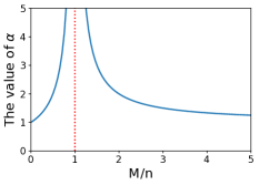
(a) The variance factor $\alpha$ w.r.t. $M/n$

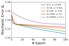
(b) Stochastic error vs. factors $b,\gamma$ and $t$

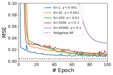
(c) MSE vs. the factors $b,\gamma$ and $t$

Figure 1: (a) The variance factor $\alpha$ w.r.t. ratio $M/n$, which make the variance explores near the transition point $M=n$. (b) Empirical stochastic gradient errors $\Delta_{t}=\frac{1}{n}\sum_{i=1}^{n}|\widehat{f}_{M,b,t}({\boldsymbol{x}}_{i})-\widehat{f}_{M}({\boldsymbol{x}}_{i})|$ of the ridgeless RF-SGD predictors on $n=10000$ synthetic examples. (c) The test MSE of all ridgeless RF-SGD estimators.

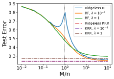
(a) Test errors v.s. regulerizations

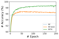
(b) Test accuracies of compared methods

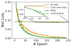
(c) Training loss and the kernel trace

Figure 2: (a) Test errors of the RF predictors (solid lines) and kernel predictors (dashed lines) w.r.t. different regularization. Note that, the ridgeless RF predictors exhibit a double descent curve. (b) Test accuracies of the compared methods on the MNIST dataset. (c) Training loss (solid lines) and the trace of kernel $\text{Tr}(\mathbf{K})$ (dashed lines) of the RF predictors on the MNIST dataset.

	Kernel Ridge	Kernel Ridgeless	RF	RF-SGD	RFTK
dna	52.83$\pm$1.66	49.67$\pm$18.54	52.83$\pm$1.66	51.33$\pm$1.89	92.92$\pm$0.89
letter	96.54$\pm$0.25	96.40$\pm$0.15	95.33$\pm$0.32	91.74$\pm$0.46	96.17$\pm$0.29
pendigits	97.46$\pm$0.42	90.67$\pm$4.75	96.91$\pm$0.43	46.04$\pm$5.62	98.64$\pm$0.43
segment	82.99$\pm$1.85	56.71$\pm$10.71	83.44$\pm$1.69	37.75$\pm$9.11	94.55$\pm$1.52
satimage	90.43$\pm$0.48	88.79$\pm$0.77	87.67$\pm$0.89	90.33$\pm$1.36	90.79$\pm$1.23
usps	92.49$\pm$0.70	87.47$\pm$7.38	94.38$\pm$0.60	49.81$\pm$3.52	97.29$\pm$0.61
svmguide2	81.90$\pm$2.78	70.13$\pm$4.91	66.20$\pm$4.64	81.65$\pm$4.25	82.78$\pm$4.84
vehicle	63.00$\pm$2.80	79.35$\pm$2.89	75.94$\pm$2.88	74.24$\pm$3.92	80.06$\pm$4.49
wine	39.17$\pm$6.27	48.89$\pm$13.68	91.11$\pm$19.40	43.89$\pm$6.19	98.33$\pm$1.36
shuttle	/	/	79.08$\pm$26.76	98.94$\pm$0.48	99.63$\pm$0.19
Sensorless	/	/	32.92$\pm$8.22	17.72$\pm$3.84	86.10$\pm$0.73
MNIST	/	/	95.52$\pm$0.16	96.61$\pm$0.11	98.09$\pm$0.07

Table 1: Classification accuracy (%) for classification datasets. We bold the results with the best method and underline the ones that are not significantly worse than the best one.

Theoretical findings illustrate that smaller trace of kernel matrix $\text{Tr}(\mathbf{K})$ can lead to better performance. We first propose a bi-level optimization learning problem

$$\min_{{\boldsymbol{w}}} \frac{1}{n}\sum_{i=1}^{n}\left({\boldsymbol{w}}^{\top}\phi({\boldsymbol{x}}_{i})-y_{i}\right)^{2}$$ (9)

s.t. $${\boldsymbol{\Omega}}^{*}=\operatornamewithlimits{arg\,min}_{{\boldsymbol{\Omega}}}~{}\|\phi({\boldsymbol{X}})\|_{F}^{2}.$$

The above objective includes two steps: 1) given a certain kernel, i.e. the frequency matrix ${\boldsymbol{\Omega}}=[{\boldsymbol{\omega}}_{1},\cdots,{\boldsymbol{\omega}}_{M}]\sim\pi({\boldsymbol{w}})$, the algorithm train the ridgeless RF model ${\boldsymbol{w}}$; 2) given a trained RF model ${\boldsymbol{w}}$, the algorithm optimize the spectral density (the kernel) by updating the frequency matrix ${\boldsymbol{\Omega}}$.

To accelerate the solve of (9), we optimize ${\boldsymbol{w}}$ and ${\boldsymbol{\Omega}}$ jointly by minimize the the following objective

$$\mathcal{L}({\boldsymbol{w}},{\boldsymbol{\Omega}})=\frac{1}{n}~{}\sum_{i=1}^{n}\left(f({\boldsymbol{x}}_{i})-{\boldsymbol{y}}_{i}\right)^{2}+\beta\|\phi(\boldsymbol{X})\|_{F}^{2},$$ (10)

where $\beta$ is a hyperparameter to balance the effect between empirical loss and the trace of kernel matrix. Here, the update of ${\boldsymbol{w}}$ is still only dependent on the squared loss (thus it is still ridgeless), but the update of ${\boldsymbol{\Omega}}$ is related to both the squared loss and Frobenius norm.

Therefore, the time complexity for update ${\boldsymbol{w}}$ once is $\mathcal{O}(Mb)$. However, since the trace is defined on all data, the update of ${\boldsymbol{\Omega}}$ is relevant to all data and time complexity is $\mathcal{O}(nMd)$, which is infeasible to update in every iterations. Meanwhile, the kernel needn’t to update frequently, and thus we apply an asynchronous strategy for optimizing the spectral density. As shown in Algorithm 1, the frequency matrix ${\boldsymbol{\Omega}}$ is updated after every $s$ iterations for the update of ${\boldsymbol{w}}$. The total complexity for the asynchronous strategy is $\mathcal{O}(nMdT/s)$.

6 Experiments

We use random Fourier feature defined in (8) to approximate the Gaussian kernel $K({\boldsymbol{x}},{\boldsymbol{x}}^{\prime})=\exp(-\sigma^{2}\|{\boldsymbol{x}}-{\boldsymbol{x}}^{\prime}\|^{2}/2)$. Note that, the corresponding random Fourier features (8) is with the frequency matrix ${\boldsymbol{\Omega}}\sim\mathcal{N}(0,\sigma^{2})$. We implement all code on Pytorch and tune hyperparameters over $\sigma^{2}\in\{0.01,\cdots,1000\}$, $\lambda=\{0.1,\cdots,10^{-5}\}$ by grid search.

6.1 Numerical Validations

6.1.1 Factors of Stochastic Gradient Methods

We start with a nonlinear problem $y=\min(-{\boldsymbol{w}}^{\top}{\boldsymbol{x}},{\boldsymbol{w}}^{\top}{\boldsymbol{x}})+\epsilon$, where $\epsilon\sim\mathcal{N}(0,0.2)$ is the label noise, and ${\boldsymbol{x}}\sim\mathcal{N}(0,\mathbf{I})$. Setting $d=10$, we generate $n=10000$ samples for training and $2500$ samples for testing. The optimal kernel hyperparameter is $\sigma^{2}=100$ after grid search.

As stated in Theorem 1, the stochastic gradients error is determined by the batch size $b$, learning rate $\gamma$ and the iterations $t$. To explore effects of these factors, we evaluate the approximation between the ridgeless RF-SGD estimator $\widehat{f}_{M,b,t}$ and the ridgeless RF estimator $\widehat{f}_{M}$ on the simulated data. Given a batch size $b$, we tune the learning rate $\gamma$ w.r.t. the MSE over $\gamma\in\{10^{1},10^{0},\cdots,10^{-4}\}$. As shown in Figure 1 (b), (c), give the $b,\gamma$, we estimate the ideal iterations $t=\text{\# Epoch}*10000/b$ after which the error drops slowly As the step size $b$ increases, the learning rates $\gamma$ become larger while the iterations reduces. This coincides with the tradeoffs among these factors $b/\gamma+1/(\gamma t)$ in Theorem 1, where the balance between $b/\gamma$ and $1/\gamma t$ leads to better performance.

Comparing Figure 1 (b) and (c), we find that: 1) After the same passes over the data (same epoch), the stochastic gradient error and MSE of the algorithms with smaller batch sizes are smaller with faster drop speeds. 2) The stochastic error still decreases after the MSE converges, where the other error terms dominates the excess risk, i.e. bias of predictors.

6.1.2 Double Descent Curve in Random Features

To characterize different behaviors of the random features error w.r.t. $M$, we fixed the number of training examples $n$ and changes the random features dimensional $M$. Figure 2 (a) reports test errors in terms of different ratios $M/n$, illustrating that: 1) Kernel methods with smaller regularization lead to smaller test errors, and the reason may be regularization hurts the performance when the training data is ”clean”. 2) Test errors of RF predictors converges to the corresponding kernel predictors, because a larger $M$ have better approximation to the kernel. This coincides with Theorem 2 and 3 that a larger $M$ reduces the random features error. 3) When the regularization term $\lambda$ is small, the predictors leads to double descent curves and $M=n$ is the transition point dividing the underparamterized and overparameterized regions. The smaller regularity, the more obvious curve the RF predictor exhibits.

In the overparameterized case, the error of RF predictor converges to corresponding kernel predictor as $M$ increases, verifying the results in Theorem 2 that the variance term reduces given more features when $M>n$. In the underparamterized regime, the errors of RF predictors drop first and then increase, and finally explodes at $M=n$. These empirical results validates theoretical findings in Theorem 3 that the variance term dominates the random features near $M=n$ and it is significantly large as shown in Figure 1 (a).

Methods	Time	Density	Regularizer
Kernel Ridge	$\mathcal{O}(n^{3})$	Assigned	Ridge
Kernel Ridgeless	$\mathcal{O}(n^{3})$	Assigned	Ridgeless
RF	$\mathcal{O}(nM^{2}+M^{3})$	Assigned	Ridgeless
RF-SGD	$\mathcal{O}(MbT)$	Assigned	Ridgeless
RFTK	$\mathcal{O}(nMbT/s)$	Learned	$\|\phi({\boldsymbol{X}})\|_{F}^{2}$

Table 2: Compared algorithms.

6.1.3 Benefits from Tunable Kernel

Motivated by the theoretical findings that the trace of kernel matrix $\text{Tr}(\mathbf{K})$ influences the performance, we design a tunable kernel method RFTK that adaptively optimizes the spectral density in the training. To explore the influence of factors upon convergence, we evaluate both test accuracy and training loss on the MNIST dataset. Compared with the exact random features (RF) and random features with stochastic gradients (RF-SGD), we conduct experiments on the entire MNIST datasets. From Figure 2 (b), we find there is a significant accuracy gap between RF-SGD and RFTK. Figure 2 (c) indicates the trace of kernel matrix term takes affects after the current model fully trained near $100$ epochs, and it decrease fast. Specifically, since the kernel is continuously optimized, more iterations can still improve the its generalization performance, while the accuracy of RF-SGD decreases after $100$ epochs because of the overfitting to the given hypothesis.

Figure 2 (b) and (c) explain the benefits from the penalty of $\text{Tr}(\mathbf{K})$ that optimizes the kernel during the training, avoiding kernel selection. Empirical studies shows that smaller $\text{Tr}(\mathbf{K})$ guarantees better performance, coinciding with the theoretical results in Theorem 1 and Theorem 3 that both stochastic gradients error and random features error depends on $\text{Tr}(\mathbf{K})$.

6.2 Empirical Results

Compared with related algorithms listed in Table 2, we evaluate the empirical behavior of our proposed algorithm RFTK on several benchmark datasets. Only the kernel ridge regression makes uses of the ridge penalty $\|{\boldsymbol{w}}\|_{2}^{2}$, while the others are ridgeless. For the sake of presentation, we perform regression algorithms on classification datasets with one-hot encoding and cross-entropy loss. We set $b=32$ and $100$ epochs for the training, and thus the stop iteration is $T=100n/32$. Before the training, we tune the hyperparameters $\sigma^{2},\lambda,\gamma,\beta$ via grid search for algorithms on each dataset. To obtain stable results, we run methods on each dataset 10 times with randomly partition such that 80% data for training and $20\%$ data for testing. Further, those multiple test errors allow the estimation of the statistical significance among methods.

Table 1 reports the test accuracies for compared methods over classification tasks. It demonstrates that: 1) In some cases, the proposed RFTK remarkably outperforms the compared methods, for example dna, segment and Sensorless. That means RFTK can optimize the kernel even with a bad initialization, which makes it more flexible than the schema (kernel selection + learning). 2) For many tasks, the accuracies of RFTK are also significantly higher than kernel predictors, i.e. dna, because the learned kernel is more suitable for these tasks. 3) Compared to kernel predictors, RFTK leads to similar or worse results in some cases. The reason is that kernel hyperparameter $\sigma^{2}$ has been tuned and in these cases they are near the optimal one, and thus the spectral density is changed a little by RFTK.

7 Conclusion

We study the generalization properties for ridgeless regression with random features, and devise a kernel learning algorithm that asynchronously tune spectral kernel density during the training. Our work filled the gap between the generalization theory and practical algorithms for ridgeless regression with random features. The techniques presented here provides theoretical and algorithmic insights for understanding of neural networks and designing new algorithms.

Appendix A Proofs

In this section, we provide brief proofs for Theorem 1 and Theorem 3, respectively.

Proof for Theorem 1.

We introduce gradient descent algorithm for random features $\widehat{f}_{M,t}({\boldsymbol{x}})=\langle{\boldsymbol{v}}_{t},\phi({\boldsymbol{x}})\rangle,~{}\text{with}$ with ${\boldsymbol{v}}_{1}=0$ and

$${\boldsymbol{v}}_{t+1}={\boldsymbol{v}}_{t}-\frac{\gamma_{t}}{n}\sum_{i=1}^{n}\left(\langle{\boldsymbol{v}}_{t},\phi({\boldsymbol{x}}_{i})\rangle-y_{i}\right)\phi({\boldsymbol{x}}_{i}).$$ (11)

By (LABEL:eq.error_decomposition), we consider the decomposition

$$\|\widehat{f}_{M,b,t}-\widehat{f}_{M}\|\leq\|\widehat{f}_{M,b,t}-\widehat{f}_{M,t}\|+\|\widehat{f}_{M,t}-\widehat{f}_{M}\|.$$ (12)

From Lemma 5 in Carratino et al. [2018], under Assumptions 1, 2, let $\delta\in(0,1)$, $\gamma\leq\frac{n}{9T\log\frac{n}{\delta}}\wedge\frac{1}{8(1+\log T)}$ and $n\geq 32\log^{2}\frac{2}{\delta}$, the following bounded holds with the probability $1-2\delta$

$$\|\widehat{f}_{M,b,t}-\widehat{f}_{M,t}\|_{L^{2}(\mu)}^{2}\leq 208Bp\left(\frac{\gamma}{b}\right).$$ (13)

Setting $\gamma_{t}=\gamma$, one can derive the closed-form solution for stochastic gradient

$$\widehat{f}_{M,t}({\boldsymbol{x}})=\phi({\boldsymbol{x}})\sum_{l=0}^{t-1}\left[I-\frac{\gamma}{n}\phi({\boldsymbol{X}})^{\top}\phi({\boldsymbol{X}})\right]^{l}\frac{\gamma}{n}\phi({\boldsymbol{X}})^{\top}{\boldsymbol{y}}$$

By the identity $\sum_{\tau=0}^{t-1}(1-Z)^{\tau}Z=I-(I-Z)^{t}$, we get that

$$\widehat{f}_{M,t}({\boldsymbol{x}}) =\phi({\boldsymbol{x}})\sum_{l=0}^{t-1}\left[I-\frac{\gamma}{n}\phi({\boldsymbol{X}})^{\top}\phi({\boldsymbol{X}})\right]^{l}\left(\frac{\gamma}{n}\phi({\boldsymbol{X}})^{\top}\phi({\boldsymbol{X}})\right)$$

$$\quad\left(\frac{\gamma}{n}\phi({\boldsymbol{X}})^{\top}\phi({\boldsymbol{X}})\right)^{-1}\frac{\gamma}{n}\phi({\boldsymbol{X}})^{\top}{\boldsymbol{y}}$$

$$=\phi({\boldsymbol{x}})\left[I-\left(I-\frac{\gamma}{n}\phi({\boldsymbol{X}})^{\top}\phi({\boldsymbol{X}})\right)^{t}\right]$$

$$\quad\left(\phi({\boldsymbol{X}})^{\top}\phi({\boldsymbol{X}})\right)^{-1}\phi({\boldsymbol{X}})^{\top}{\boldsymbol{y}}.$$

Denote the kernel operator $\mathbf{K}_{M}=\phi({\boldsymbol{X}})\phi({\boldsymbol{X}})^{\top}$. Using the identity $(Z^{\top}Z)^{-1}Z=(Z^{\top}Z)^{-1}Z(ZZ^{\top})(ZZ^{\top})^{-1}=Z^{\top}(ZZ^{\top})^{-1}$ for any matrix $Z$, we have

$$|\widehat{f}_{M,t}({\boldsymbol{x}})-\widehat{f}_{M}({\boldsymbol{x}})|$$ (14)

$$= \Bigg{|}\phi({\boldsymbol{x}})\left(I-\frac{\gamma}{n}\phi({\boldsymbol{X}})^{\top}\phi({\boldsymbol{X}})\right)^{t}\left(\phi({\boldsymbol{X}})^{\top}\phi({\boldsymbol{X}})\right)^{-1}\phi({\boldsymbol{X}})^{\top}{\boldsymbol{y}}\Bigg{|}$$

$$= \Bigg{|}\phi({\boldsymbol{x}})\left(I-\frac{\gamma}{n}\phi({\boldsymbol{X}})^{\top}\phi({\boldsymbol{X}})\right)^{t}\phi({\boldsymbol{X}})^{\top}\left(\phi({\boldsymbol{X}})\phi({\boldsymbol{X}})^{\top}\right)^{-1}{\boldsymbol{y}}\Bigg{|}$$

$$= \Bigg{|}\phi({\boldsymbol{x}})\phi({\boldsymbol{X}})^{\top}\left(I-\frac{\gamma}{n}\mathbf{K}_{M}\right)^{t}\left(\mathbf{K}_{M}\right)^{-1}{\boldsymbol{y}}\Bigg{|}$$

Consider the eigenvalue decomposition for kernel matrix

$$\frac{1}{n}\mathbf{K}_{M}=U\Lambda U^{\top},$$

where $UU^{\top}=U^{\top}U=I$ records the eigenvectors and $\Lambda$ is a $n\times n$ diagonal with eigenvalues. Consequently,

$$\left(I-\frac{\gamma}{n}\mathbf{K}_{M}\right)^{t}=\left[U^{-1}U-\frac{\gamma}{n}U^{-1}\Lambda U\right]^{t}=U^{-1}\left[I-\frac{\gamma}{n}\Lambda\right]^{t}U.$$

Then, it holds

$$\left\|\phi({\boldsymbol{X}})^{\top}\left(I-\gamma\mathbf{K}_{M}\right)^{t}\right\|^{2}_{2}$$ (15)

$$\leq \left\|\phi({\boldsymbol{X}})^{\top}\left(I-\gamma\mathbf{K}_{M}\right)^{t}\right\|^{2}_{2}$$

$$\leq \left\|\phi({\boldsymbol{X}})^{\top}U^{-1}\left[I-\gamma\Lambda\right]^{t}\right\|_{2}^{2}\big{\|}U\big{\|}_{2}^{2}$$

$$\leq \left\|\left[I-\gamma\Lambda\right]^{t}U^{-1}K(U^{-1})\left[I-\gamma\Lambda\right]^{t}\right\|_{2}$$

$$= \left\|\left[I-\gamma\Lambda\right]^{t}U\left[I-\gamma\Lambda\right]^{t}\right\|_{2}$$

$$= \max_{j\in[n]}(1-\gamma\Lambda_{jj})^{2t}\Lambda_{jj}$$

$$\leq \frac{1}{2e\gamma t},$$

where $\Lambda_{jj}$ is the $j$-th eigenvalue in the diagonal of $\Lambda$.

Substituting (LABEL:eq.proof.iteration) to (LABEL:eq.proof.gd_rf), we have

$$\|\widehat{f}_{M,t}-\widehat{f}_{M}\|^{2}_{L^{2}(\mu)}$$ (16)

$$\leq \|\phi({\boldsymbol{x}})\|^{2}\left\|\phi({\boldsymbol{X}})^{\top}\left(I-\frac{\gamma}{n}\mathbf{K}_{M}\right)^{t}\right\|^{2}\|{\boldsymbol{y}}\|_{K^{-1}}$$

$$\leq \frac{\kappa^{2}}{2e\gamma t}\|{\boldsymbol{y}}\|_{K^{-1}}.$$

Here, $\|{\boldsymbol{y}}\|_{K^{-1}}$ denote the inverse kernel norm of the labels defined as $\|{\boldsymbol{y}}\|_{K^{-1}}={\boldsymbol{y}}^{\top}(K({\boldsymbol{X}},{\boldsymbol{X}}))^{-1}{\boldsymbol{y}}$. According to Schölkopf et al. [1998], it holds $\|{\boldsymbol{y}}\|_{K^{-1}}\leq\|f^{*}\|_{K}$ under the assumption that the true regression $f^{*}({\boldsymbol{x}})=\langle f^{*},K_{{\boldsymbol{x}}}\rangle$ lies in the RKSH of the kernel $K$, i.e., $f^{*}\in{\mathcal{H}_{K}}$.

Substituting (13) and (LABEL:eq.rfgd_rf) to (12), we prove the result. ∎

Proof of Theorem 2.

The Ridgeless RF predictor admits the bias-variance decomposition

$$\mathbb{E}\mathcal{E}(\widehat{f}_{M})=\mathcal{E}\left[\mathbb{E}~{}(\widehat{f}_{M})\right]+\mathbb{E}\left[\text{Var}(\widehat{f}_{M})\right].$$

And thus, the random features error have

$$\mathbb{E}\mathcal{E}(\widehat{f}_{M})-\mathcal{E}(\widehat{f})=\left\|\mathbb{E}~{}(\widehat{f}_{M})-\widehat{f}\right\|_{L^{2}(\mu)}^{2}+\mathbb{E}\left[\text{Var}(\widehat{f}_{M})\right].$$ (17)

We estimate these two terms, respectively. From Proposition 3.1, one can obtain

$$\mathbb{E}~{}\big{[}\widehat{f}_{M}({\boldsymbol{x}})\big{]}=K({\boldsymbol{x}},{\boldsymbol{X}})K({\boldsymbol{X}},{\boldsymbol{X}})^{\dagger}{\boldsymbol{y}}=\widehat{f}({\boldsymbol{x}}).$$ (18)

Thus, we only need to bound the variance in the overparameterized case. From Proposition C.15 Jacot et al. [2020], the variance of ridgeless RF predictor can be bounded by

$$\mathbb{E}\left[\text{Var}(\widehat{f}_{M})\right]\leq\frac{(\alpha+c_{1})\kappa\|{\boldsymbol{y}}\|^{2}_{K^{-1}}}{M},$$ (19)

where $\alpha$ is some constant related to $M/n$. From Proposition C.11 and $\tilde{\lambda}=0$, we obtain $\alpha=\frac{M/n}{M/n-1}$ when $M\geq n$.

By substituting (18) and (19) to (17), we prove the result. ∎

Proof of Theorem 3.

Theorem 4.1 in Jacot et al. [2020] provided the approximate between the ridge RF estimator and the ridge regression estimator, we make the RF estimator to the ridgeless case. Theorem 4.1 provided that

$$|\mathbb{E}\widehat{f}_{M,\tilde{\lambda}}({\boldsymbol{x}})-\widehat{f}_{\lambda}({\boldsymbol{x}})|\leq\frac{c\sqrt{K({\boldsymbol{x}},{\boldsymbol{x}})}\|{\boldsymbol{y}}\|_{K^{-1}}}{M}$$ (20)

with the effective ridge $\tilde{\lambda}$ satisfying

$$\lambda=\tilde{\lambda}+\frac{{\lambda}}{M/n}\sum_{i=1}^{n}\frac{d_{i}}{{\lambda}+d_{i}}$$

where $d_{i}$ is the $j$-th element on diagonal form of $\mathbf{K}$. We consider the ridgeless RF case with $\tilde{\lambda}=0$, such that

$$\frac{M}{n}=\frac{1}{n}\sum_{i=1}^{n}\frac{d_{i}}{\lambda+d_{i}}=\frac{1}{n}\text{Tr}\left[\mathbf{K}(\mathbf{K}+\lambda I)^{-1}\right].$$

From the proof of Proposition C.7 in Jacot et al. [2020], the constant is $c=\left(\frac{\text{Tr}(\mathbf{K})}{M}\right)^{2}$. Using Assumption 1, we have $\sqrt{K({\boldsymbol{x}},{\boldsymbol{x}})}\leq\kappa$ Substituting the estimate for $\lambda,c,\sqrt{K({\boldsymbol{x}},{\boldsymbol{x}})}$ to (20), we obtain

$$\left\|\mathbb{E}[\widehat{f}_{M}]-\widehat{f}_{\lambda}\right\|_{L^{2}(\mu)}^{2}\leq\frac{\kappa^{2}\text{Tr}(\mathbf{K})^{4}\|{\boldsymbol{y}}\|_{K^{-1}}^{2}}{M^{6}}.$$ (21)

From Proposition C.15 Jacot et al. [2020], the variance of ridgeless RF predictor can be bounded by

$$\mathbb{E}\left[\text{Var}(\widehat{f}_{M})\right]\leq\frac{(\alpha+c_{1})\kappa\|{\boldsymbol{y}}\|^{2}_{K^{-1}}}{M},$$ (22)

where $\alpha$ is related to $M/n$. From Proposition C.11, setting $\tilde{\lambda}=0$, we obtain $\alpha=\frac{1}{1-M/n}$ when $M<n$.

By substituting (21) and (22) to (17), we prove the result. ∎

References

- Advani et al. [2020] Madhu S Advani, Andrew M Saxe, and Haim Sompolinsky. High-dimensional dynamics of generalization error in neural networks. Neural Networks, 132:428–446, 2020.
- Bartlett et al. [2005] Peter L. Bartlett, Olivier Bousquet, and Shahar Mendelson. Local Rademacher complexities. The Annals of Statistics, 33(4):1497–1537, 2005.
- Bartlett et al. [2020] Peter L Bartlett, Philip M Long, Gábor Lugosi, and Alexander Tsigler. Benign overfitting in linear regression. Proceedings of the National Academy of Sciences, 117(48):30063–30070, 2020.
- Belkin et al. [2018] Mikhail Belkin, Siyuan Ma, and Soumik Mandal. To understand deep learning we need to understand kernel learning. arXiv preprint arXiv:1802.01396, 2018.
- Caponnetto and De Vito [2007] Andrea Caponnetto and Ernesto De Vito. Optimal rates for the regularized least-squares algorithm. Foundations of Computational Mathematics, 7(3):331–368, 2007.
- Carratino et al. [2018] Luigi Carratino, Alessandro Rudi, and Lorenzo Rosasco. Learning with sgd and random features. In Advances in Neural Information Processing Systems 31 (NeurIPS), pages 10192–10203, 2018.
- Geiger et al. [2020] Mario Geiger, Arthur Jacot, Stefano Spigler, Franck Gabriel, Levent Sagun, Stéphane d’Ascoli, Giulio Biroli, Clément Hongler, and Matthieu Wyart. Scaling description of generalization with number of parameters in deep learning. Journal of Statistical Mechanics: Theory and Experiment, 2020(2):023401, 2020.
- Ghorbani et al. [2021] Behrooz Ghorbani, Song Mei, Theodor Misiakiewicz, and Andrea Montanari. Linearized two-layers neural networks in high dimension. The Annals of Statistics, 49(2):1029–1054, 2021.
- Hastie et al. [2019] Trevor Hastie, Andrea Montanari, Saharon Rosset, and Ryan J Tibshirani. Surprises in high-dimensional ridgeless least squares interpolation. arXiv preprint arXiv:1903.08560, 2019.
- Jacot et al. [2020] Arthur Jacot, Berfin Simsek, Francesco Spadaro, Clément Hongler, and Franck Gabriel. Implicit regularization of random feature models. In International Conference on Machine Learning, pages 4631–4640. PMLR, 2020.
- Li and Liu [2022] Jian Li and Yong Liu. Optimal rates for distributed learning with random features. In Proceedings of the 31st International Joint Conference on Artificial Intelligence (IJCAI), 2022.
- Li et al. [2018] Jian Li, Yong Liu, Rong Yin, Hua Zhang, Lizhong Ding, and Weiping Wang. Multi-class learning: From theory to algorithm. In Advances in Neural Information Processing Systems 31, pages 1591–1600, 2018.
- Li et al. [2019] Jian Li, Yong Liu, Rong Yin, and Weiping Wang. Multi-class learning using unlabeled samples : Theory and algorithm. In Proceedings of the 28th International Joint Conference on Artificial Intelligence (IJCAI), 2019.
- Li et al. [2020] Jian Li, Yong Liu, and Weiping Wang. Automated spectral kernel learning. In Thirty-Four AAAI Conference on Artificial Intelligence, 2020.
- Liang and Rakhlin [2020] Tengyuan Liang and Alexander Rakhlin. Just interpolate: Kernel “ridgeless” regression can generalize. The Annals of Statistics, 48(3):1329–1347, 2020.
- Mei and Montanari [2019] Song Mei and Andrea Montanari. The generalization error of random features regression: Precise asymptotics and the double descent curve. Communications on Pure and Applied Mathematics, 2019.
- Nakkiran et al. [2021] Preetum Nakkiran, Gal Kaplun, Yamini Bansal, Tristan Yang, Boaz Barak, and Ilya Sutskever. Deep double descent: Where bigger models and more data hurt. Journal of Statistical Mechanics: Theory and Experiment, 2021(12):124003, 2021.
- Rahimi and Recht [2007] Ali Rahimi and Benjamin Recht. Random features for large-scale kernel machines. In Advances in Neural Information Processing Systems 21 (NIPS), pages 1177–1184, 2007.
- Rahimi and Recht [2008] Ali Rahimi and Benjamin Recht. Weighted sums of random kitchen sinks: Replacing minimization with randomization in learning. In Advances in Neural Information Processing Systems 22 (NIPS), pages 1313–1320, 2008.
- Rudi and Rosasco [2017] Alessandro Rudi and Lorenzo Rosasco. Generalization properties of learning with random features. In Advances in Neural Information Processing Systems 30 (NIPS), pages 3215–3225, 2017.
- Rudi et al. [2018] Alessandro Rudi, Daniele Calandriello, Luigi Carratino, and Lorenzo Rosasco. On fast leverage score sampling and optimal learning. In Advances in Neural Information Processing Systems, pages 5672–5682, 2018.
- Schölkopf et al. [1998] Bernhard Schölkopf, Alexander Smola, and Klaus-Robert Müller. Nonlinear component analysis as a kernel eigenvalue problem. Neural computation, 10(5):1299–1319, 1998.
- Smale and Zhou [2007] Steve Smale and Ding-Xuan Zhou. Learning theory estimates via integral operators and their approximations. Constructive approximation, 26(2):153–172, 2007.
- Zhang et al. [2021] Chiyuan Zhang, Samy Bengio, Moritz Hardt, Benjamin Recht, and Oriol Vinyals. Understanding deep learning (still) requires rethinking generalization. Communications of the ACM, 64(3):107–115, 2021.