Direct closed-loop identification of continuous-time systems
using fixed-pole observer model*

Abstract

This paper provides a method for obtaining a continuous-time model of a target system in a closed-loop environment from input-output data alone. The proposed method is based on a fixed-pole observer model, which is a reasonable continuous-time version of the innovation model in discrete-time and allows the identification of unstable target systems in closed-loop environments with unknown controllers. The method is within the framework of the stabilized output error method and shares usability advantages such as robustness to noise with complex dynamics and applicability to a wide class of models, in addition to advantages derived from continuous-time models such as tolerance to system stiffness and easy access to physical knowledge. The effectiveness of the method is illustrated through numerical examples.

I INTRODUCTION

System modeling is the foundation of control system design, and among them, closed-loop identification is often necessary for practical use. When the target system is open-loop unstable, closed-loop identification must be performed after stabilizing the system with some feedback. Even if the system itself is stable, it is often required to identify it in a closed-loop environment for industrial applications from the viewpoint of economic efficiency and safety. Furthermore, in large-scale networked systems, which have been attracting much attention in recent years, each subsystem must be identified within the network, and closed-loop identification is inevitable because of the presence of feedback from other subsystems. In this case, it is not possible to obtain accurate information on the feedback part. An identification method that does not require any controller information is desirable to deal with such a case. In addition, though most identification methods handle discrete-time time models, it is often desired to obtain continuous-time models because they are intuitive to most control engineers and the system parameters are consistent with physical properties.

In the conventional closed-loop identification method within the framework of the Prediction Error Method, various “direct methods” have been developed that do not require any information on the controller and perform system identification based only on the input and output data of the target system (see surveys [1, 2]). In these methods, accurate modeling of the observed noise characteristics is important in general, but it is difficult to accurately model the noise characteristics in the real world due to its complexity. In addition, although it may not be widely recognized, it is not easy to identify open-loop unstable systems [3]. On the other hand, in the framework of subspace identification methods, SSARX [4] and PBSID [5] are well known that do not require controller information and can handle unstable systems. The effectiveness of these methods has also been pointed out in a survey paper [6]. Though they may not work well in the presence of complex colored noise, a method which can overcome such shortcomings has been recently proposed [7]. What these methods have in common is that they employ an observer (or Kalman filter) form called the innovation form, which makes it easy to deal with unstable systems. However, all of these papers discuss discrete-time systems only. Hence, the data sampling time must be chosen very carefully, and we have to convert the obtained discrete-time model into a continuous-time one. Consequently, it is often not easy to obtain an accurate continuous-time model by these methods.

On the other hand, various methods to obtain a continuous-time model directly from input-output data have been actively developed (see [8, 9]). A few papers (e.g., [10, 11]) discuss closed-loop identification, but they cannot handle unstable systems without controller knowledge. One exception is the stabilized output error (OE) method proposed by the authors [12]. The method of [12] is applicable if one can find a controller that stabilizes the target system, where the controller can be different from the original one in the closed-loop. Also, its effectiveness has been demonstrated through various numerical examples. However, it is not clear how to find an appropriate stabilizing controller for the system to be identified.

This paper aims to give a method to directly identify a continuous-time model using only input/output data of a system in an uncertain closed-loop environment. Specifically, we give a method for handling the case where the controller is completely unknown in the stabilized OE method framework and propose a fixed-pole observer model, which is a reasonable continuous-time version of the innovation model in discrete-time systems. Furthermore, many variants can be created based on the idea of the proposed method, and here we propose a fixed-pole extended observer model. It can handle time-series data with non-stationary trends, similar to the ARIX and ARIMAX models for discrete-time systems.

In this paper, for a vector $x$, $x_{i}$ represents its $i$-th element, and $\mathcal{N}\left(\mu,\sigma^{2}\right)$ denotes the normal distribution with mean $\mu$ and variance $\sigma^{2}$.

II PROBLEM SETTING

We consider a closed-loop system described by the differential equation

$$y(t) =P^{\star}(p)\left(u(t)+w(t)\right)+\eta(t),$$ (1)

$$u(t) =r_{u}(t)+K(p)\left(r_{y}(t)-y(t)\right),$$ (2)

where $p$ denotes the time-domain differential operator and $P^{\star}(p)$ is the rational function of $p$ which represents the plant to be identified, and $K(p)$ represents an unknown controller which stabilizes $P^{\star}(p)$ (see the upper half of Fig. 1). The signals $u(t)$, $y(t)$, $r_{u}(t)$ and $r_{y}(t)$ are the plant input, the plant output measurement, the excitation signal and the reference signal, respectively. $r_{u}(t)$ and $r_{y}(t)$ may be unknown but are supposed to be rich enough for identification purpose. And $w(t)$ and $\eta(t)$ denote the input disturbance and the measurement noise, respectively, which may be colored.

Remark 1

For conciseness of notation, the plant and controller are SISO systems here, but the discussion for the case of MIMO systems is almost the same. $\Box$

The plant is assumed to belong to a known parametrized set

$${\cal P}:=\{P(p,\theta)~{}|~{}\theta\in\mathbb{R}^{n_{\theta}}\},$$

so it is described by $P^{\star}(p)=P(p,\theta^{\star})$ for some parameter $\theta^{\star}\in\mathbb{R}^{n_{\theta}}$. The I/O data are collected with the sampling time $h$ and given by

$${\cal Z}=\left\{u(kh),y(kh)~{}\middle|~{}k=0,1,\cdots,N-1\right\}$$ (3)

where $N$ is the data length. It is assumed that $N$ is long enough and $h$ is short enough to capture the plant dynamics. The problem here is to estimate $\theta^{\star}$ from the I/O data alone.

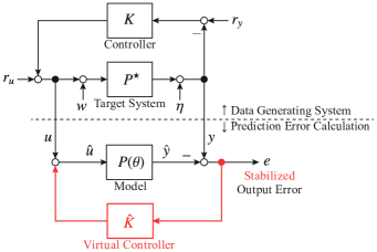
Figure 1: Data generating system and stabilized output error method

III STABILIZED OUTPUT ERROR METHODS

As a preliminary, we briefly outline the stabilized OE method framework.

III-A Output Error (OE) Method

Most natural way to identify $P(p,\theta^{\star})$ based on I/O data would be to employ the plant model described by

$$\hat{y}(t) =P(p,\theta)u(t)$$ (4)

and obtain the parameter estimate $\hat{\theta}$ by minimizing the output error

$$e(t) =y(t)-\hat{y}(t)$$ (5)

as

$$\hat{\theta}=\operatorname*{arg\,min}_{\theta}\sum_{k=0}^{N-1}e^{2}(hk).$$ (6)

Remark 2

The initial state of the model is necessary for calculating $\hat{y}(t)$. Although omitted in this paper for conciseness, these initial states are also explored simultaneously in the minimization of prediction error (6). $\Box$

The lower half of Fig. 1, excluding the virtual controller (in red), corresponds to the calculation of this output error. This is nothing but the output error method. In applications to closed-loop system identification, the estimate is biased by the correlation between $u$ and noise, but is often acceptable if the signal-to-noise ratio is high and the target plant $P^{\star}$ is stable. However, when $P^{\star}$ is unstable, this method does not work well. Because when $\theta$ takes the desired value $\theta^{\star}$, the prediction system becomes unstable and the output error $e(t)$ diverges.

III-B Stabilized OE Method

Hence, [12] has proposed the stabilized OE method, which is to employ the following form;

$$\hat{y}(t) =P(p,\theta)\hat{u}(t), \hat{u}(t) =u(t)+\hat{K}(p)e(t),$$ (7)

and (5), where $\hat{K}(p)$ is called a virtual controller which stabilizes $P(p,\theta^{\star})$. Introduction of the virtual controller with error feedback plays an essential role to handle unstable plants [12]. When $K(p)$ is known, it has been shown that $\hat{K}(p)=K(p)$ produces an unbiased plant model. More importantly, this method turns out to be quite insensitive to the discrepancy between $\hat{K}(p)$ and $K(p)$ as demonstrated in [12]. One open problem here is how to find an appropriate virtual controller when we have no clue about $K(p)$ or $P(p,\theta^{\star})$.

IV PROPOSED METHOD

Now, we give a new scheme within the framework of stabilized OE methods, which can be applied when we have no clue $K(p)$ nor $P^{\star}(p)$.

IV-A Continuous-time Innovation Model

One variant of the stabilized OE method is to set up the virtual controller so that the prediction system becomes an observer for $P(p,\theta)$. Let $A(\theta)\in\mathbb{R}^{n\times n}$, $B(\theta)\in\mathbb{R}^{n\times 1}$ and $C(\theta)\in\mathbb{R}^{1\times n}$ be matrices of a minimal state space representation of $P(p,\theta)$, namely

$$P(p,\theta)=C(\theta)\left(pI-A(\theta)\right)^{-1}B(\theta).$$ (8)

For this system, an observer can be constructed as

$$\dot{\hat{x}}(t) =A(\theta)\hat{x}(t)+B(\theta)u(t)+\hat{K}_{\hat{x}}e(t)$$ (9a)

$$\hat{y}(t) =C(\theta)\hat{x}(t)$$ (9b)

$$e(t) =y(t)-\hat{y}(t)$$ (9c)

where $\hat{K}_{\hat{x}}\in\mathbb{R}^{n\times 1}$ is an observer gain.

A straightforward approach when $K(p)$ is unknown is to search for $\hat{K}_{\hat{x}}$ simultaneously with $\theta$ by solving

$$\operatorname*{minimize}_{\theta,\hat{K}_{\hat{x}}}\sum_{k=0}^{N-1}e^{2}(hk).$$ (10)

In fact, the model corresponding to (9) in discrete-time is called the innovation model, and optimization (10) yields the Kalman filter that embed the plant system $P^{\star}$.

Remark 3

To be precise, (8) need not be a minimal realization but a realization that can accommodate the noise model in the uncontrolled mode, for the Kalman filter to be formed. Since the dynamics of noise in the real world are generally higher-order, prediction error methods (based on innovation models) require higher-order models. This is a factor that makes prediction error methods more prone to failure than output error methods (which do not require a noise model for consistency). $\Box$

However, for the continuous-time model, there is a trivial solution of (10) that takes $\hat{K}_{\hat{x}}$ extremely large and makes $e(t)\to 0$ regardless of $\theta$, and this approach does not work.

IV-B Fixed-pole observer model

To address this problem, we propose an approach that automatically adjusts $\hat{K}_{\hat{x}}$ according to model $P(p,\theta)$. More specifically, the appropriate closed-loop poles of the prediction system, i.e., the observer poles, are set in advance, and $\hat{K}_{\hat{x}}(\theta)$ is determined by the pole placement method for $P(p,\theta)$ throughout the optimization of $\theta$. This keeps the prediction system stable during the optimization process and prevents the optimization from falling into the trivial solution.

To summarize, the proposed method assumes that a set of desired observer poles $\bm{p}_{\mathrm{ob}}$ is given, and the stabilized output error is calculated by

$$\dot{\hat{x}}(t) =A(\theta)\hat{x}(t)+B(\theta)u(t)+\hat{K}_{\hat{x}}(\theta)e(t)$$ (11)

with (9b) and (9c), where the value of $\hat{K}_{\hat{x}}(\theta)$ is calculated from $\theta$ using the pole placement algorithm (e.g., the algorithm in [13]) so that the eigenvalues of $A(\theta)-\hat{K}_{\hat{x}}(\theta)C(\theta)$ are $\bm{p}_{\mathrm{ob}}$. The parameter estimate $\hat{\theta}$ is then obtained by the optimization (6).

IV-C Fixed-pole extended observer model

While there are many possible variations on how to provide stability to the predictive system in the design of virtual controllers, we introduce one noteworthy and useful variant.

Here we configure the virtual controller as follows so that the prediction system is an extended observer

$$\dot{\hat{x}}(t) =A(\theta)\hat{x}(t)+B(\theta)\left(u(t)+d(t)\right)+\hat{K}_{\hat{x}}(\theta)e(t)$$ (12a)

$$\dot{d}(t) =\hat{K}_{d}(\theta)e(t)$$ (12b)

$$\hat{y}(t) =C(\theta)\hat{x}(t)$$ (12c)

$$e(t) =y(t)-\hat{y}(t)$$ (12d)

where $d(t)$ is introduced as an input correction term and $\hat{K}_{d}\in\mathbb{R}$ is the corresponding observer gain, which will compensate the unknown offsets in $u(t)$ and $y(t)$. As in the previous model, the observer gain $\left[\hat{K}_{\hat{x}}(\theta)^{\top},\hat{K}_{d}(\theta)^{\top}\right]^{\top}$ is computed from $\theta$ so that the pole of the extended observer, i.e., the eigenvalue of $\begin{bmatrix}A(\theta)-\hat{K}_{\hat{x}}(\theta)C(\theta)&B(\theta)\\ -\hat{K}_{d}(\theta)C(\theta)&0\end{bmatrix}$ is at the given desired place $\bm{p}_{\mathrm{ob}}$.

The use of this model is illustrated through examples in the next section.

V SIMULATION

In this section, two numerical examples are shown to demonstrate the effectiveness of the proposed method. In the examples, 100 trials based on different random noise realizations are performed to see the statistics of the results. The Levenberg-Marquardt method, implemented in MATLAB as lsqnonlin function, was used in the optimization required by the proposed method.

V-A Identification in closed-loop systems with unknown controller

The first example is the closed-loop identification of an unstable plant and is based on the model of the actual magnetic levitation system in [14]. The data generating system is as shown in Fig. 1, and the systems are as follows:

$$P(p,\theta) =\frac{\theta_{4}}{p^{3}+\theta_{1}p^{2}+\theta_{2}p+\theta_{3}},$$ (13)

$$\theta^{\star} =[13.33,-494.4,-6593,7148]^{\top},$$ (14)

$$K(p) =\frac{$1.197\text{\times}{10}^{5}\text{\,}$(p+9.294)(p+13.99)(p+20.9)}{(p+399.9)(p+0.1)\left((p+121.5)^{2}+141.1^{2}\right)}.$$ (15)

An example of input/output data is shown in Fig. 2 as blue lines. Here, the excitation signal is a square wave with a $0.5\text{\,}\mathrm{s}$ period applied to $r_{y}$. The input/output data in the third period, when the effect of the initial state disappears, is used for system identification, and $5000(=N)$ data are sampled at intervals of $$0.1\text{\,}\mathrm{m}\mathrm{s}$(=h)$.

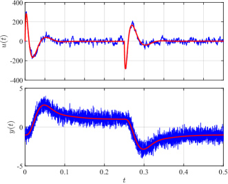
Figure 2: Example of input/output data for identification (Magnetic levitation system)

The disturbance $w(t)$ and the measurement noise $\eta(t)$ are zero-order hold signals of random numbers sampled every $0.1\text{\,}\mathrm{m}\mathrm{s}$ from $\mathcal{N}(0,0.5^{2})$, respectively. To visualize the signal-to-noise ratio, the noise-free signals are shown as red lines in Fig. 2.

Well-established methods for the closed-loop identification problem of such unstable systems include prediction error methods based on discrete-time prediction models such as ARX, ARMAX, and Box-Jenkins models. However, the system identification based on discrete-time models is prone to failure if the sampling interval and the dynamics of the target system do not match [15]. This problem is especially likely to occur in closed-loop system identification, where the sampling interval is often selected based on the requirements of the control system design. For reference, the results based on the ARMAX model, which worked best among ARX, ARMAX, and Box-Jenkins models, are shown in Fig. 3. In the figure, the frequency response of the target system is shown by the red line, and the blue lines show the characteristics of the model obtained over 100 trials based on different realizations of noise, respectively. This result was obtained with the armax function of the MATLAB System Identification Toolbox, and although the choice of model order and other settings were adjusted to obtain the best results, the results are not good. As seen in this example, there are a wide range of situations where system identification based on discrete-time predictive models is difficult.

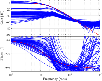
(a) ARMAX

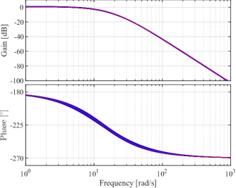
(b) Stabilized OE ($\hat{K}=K$)

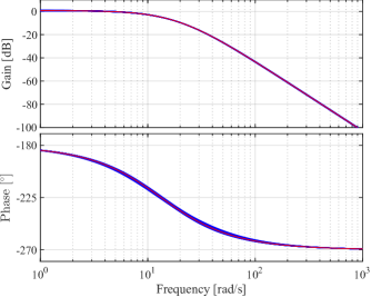
(c) Stabilized OE (fixed-pole observer model)

Figure 3: Frequency response of model

If the controller $K(p)$ is known, good identification results can be obtained by the stabilized OE method with $K(p)$ as the virtual controller $\hat{K}(p)$ as shown in Fig. 3. But this method cannot be applied without at least knowing the virtual controller that stabilizes the target system.

For the case where the controller capable of stabilizing the target system is unknown, the method proposed in this paper can be applied. For example, Fig. 3 shows the results for a virtual controller that constructs fixed-pole observer model with $\bm{p}_{\mathrm{ob}}=\left\{-3,-3\pm i\right\}$, and the results are comparable to those obtained when the controller is known (Fig. 3).

Indeed, the statistics of the parameter estimates over 100 trials are as shown in Fig. 4, and the bias in the estimates is acceptable compared to the case where $K(p)$ is known. Also, in this example, the estimate is not very sensitive to the arrangement of the poles. For example, changing the real part of the poles in $\bm{p}_{\mathrm{ob}}$ that is set to $-3$ from $-0.1$ to $-10$ hardly changes the estimates.

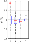
(a) Known $K$

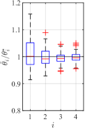
(b) Fixed-pole observer model

Figure 4: Distribution of estimates by virtual controller selection (magnetic levitation system)

This example suggests that the proposed method is effective for the problem of continuous-time system identification in a closed-loop with unknown controllers, for which no promising method is known.

V-B Non-stationary data and fixed-pole extended observer model

Real-world applications often require system identification from time-series data with non-stationary trends. Prediction error methods based on discrete-time models can deal with this type of data by using models with integrators in the noise part (e.g., ARIX and ARIMAX models). For continuous-time system identification, the fixed-pole extended observer model in Section IV-C can accommodate this type of data. And, the validity of the method is confirmed here.

In order to make a comparison with the usual OE based continuous-time system identification method, which is not applicable to closed-loop identification of unstable systems, we consider here a stable plant (Rao–Garnier test system [15, 9]) described by the following transfer function

$$P(p,\theta) =\frac{\theta_{5}p+\theta_{6}}{p^{4}+\theta_{1}p^{3}+\theta_{2}p^{2}+\theta_{3}p+\theta_{4}},$$ (16)

$$\theta^{\star} =[5,408,416,1600,-6400,1600]^{\top},$$ (17)

and data generating system is the one shown in Fig. 1 with $K=0$. To reproduce the problem in data with non-stationary trends, we set the disturbance to $w(t)=10$, and the measurement noise $\eta$ is zero-order hold signal of random numbers sampled every $1\text{\,}\mathrm{m}\mathrm{s}$ from $\mathcal{N}(0,0.4^{2})$. An example of I/O data (blue lines) and its noise-free version (red lines) are shown in Fig. 5. Note that the red and blue lines for the input $u(t)$ coincide because the plant is in an open-loop, and the disturbance $w(t)$ is not visible in $u(t)$. The effect of the constant disturbance appears as an offset in the output $y(t)$. The sampling interval is $$1\text{\,}\mathrm{m}\mathrm{s}$(=h)$, and the number of data is $$20\,000\text{\,}$(=N)$.

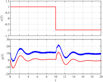
Figure 5: Example of input/output data for identification (Rao–Garnier test system with constant disturbance)

First, continuous-time models obtained with the tfest function in MATLAB System Identification Toolbox is shown in Fig. 6 for comparison. It can be seen that inappropriate models are obtained, although the conditions are sufficient for identification if there are no constant disturbances.

On the other hand, the results obtained by the stabilized OE, where the virtual controller forms the fixed-pole extended observer with $\bm{p}_{\mathrm{ob}}=\left\{-3,-3\pm i,-3\pm\frac{i}{2}\right\}$, are shown in Fig. 6. The figure shows that although some bias can be observed, appropriate models have been obtained.

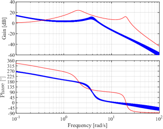
(a) Conventional (tfest)

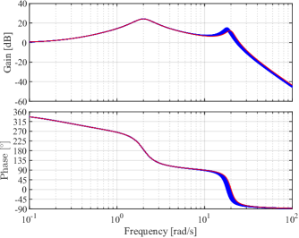
(b) Stabilized OE (fixed-pole extended observer model)

Figure 6: Frequency response of model (Rao–Garnier test system with constant disturbance)

In addition, to confirm that this approach is also valid for closed-loop identification of unstable plants, we show the results for the example in Section V-A when the disturbance is set to $w(t)=1$. Fig. 7 shows the results with the fixed-pole observer model in Section V-A, and Fig. 7 shows the results from the fixed-pole extended observer model with $\bm{p}_{\mathrm{ob}}=\left\{-3\pm i,-3\pm\frac{i}{2}\right\}$. As can be seen in the figure, there is a strong bias in the estimates from the model with no input correction term, while there is no apparent bias in the estimates from the extended observer model, confirming that the proposed method works as intended in this case as well.

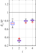
(a) Fixed-pole observer model

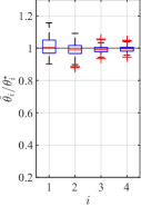
(b) Fixed-pole extended observer model

Figure 7: Distribution of estimates by virtual controller selection (magnetic levitation system with constant disturbance)

VI CONCLUSIONS

This paper has discussed closed-loop identification to obtain a continuous-time model from I/O data alone and proposed a new method. The method uses a new continuous-time prediction model named pole-fixed observer, which is a reasonable continuous-time version of the innovation model in discrete-time systems. The proposed method is also a variant of the stabilized output error method which stabilizes the prediction model by a virtual controller, and has good usability features in common with the popular output error method, such as robustness to noise with complex dynamics and applicability to a wide class of models. An important feature of the proposed method is its applicability to unstable plants in closed-loop without any knowledge of controllers, for which no promising method is yet known. Since the continuous-time model has advantages such as freedom in selecting sampling intervals and easy access to physical knowledge, it is significant that this type of system identification can be performed based on a continuous-time model. While there may be many useful variants of virtual controllers that stabilize the predictive model, we present here a case for constructing a fixed-pole expanded observer that can deal with data with non-stationary trends.

Future work includes pursuing further variations of the virtual controller and validating the idea of the proposed method in nonlinear system identification.

References

- [1] U. Forssell and L. Ljung, “Closed-loop identification revisited,” Automatica, vol. 35, no. 7, pp. 1215–1241, 1999. [Online]. Available: https://www.sciencedirect.com/science/article/pii/S0005109899000229
- [2] P. M. Van Den Hof and R. J. Schrama, “Identification and control — closed-loop issues,” Automatica, vol. 31, no. 12, pp. 1751–1770, 1995, trends in System Identification. [Online]. Available: https://www.sciencedirect.com/science/article/pii/000510989500094X
- [3] U. Forssell and L. Ljung, “Identification of unstable systems using output error and Box-Jenkins model structures,” IEEE Transactions on Automatic Control, vol. 45, no. 1, pp. 137–141, 2000.
- [4] M. Jansson, “Subspace identification and ARX modeling,” IFAC Proceedings Volumes, vol. 36, no. 16, pp. 1585–1590, 2003, 13th IFAC Symposium on System Identification (SYSID 2003), Rotterdam, The Netherlands, 27-29 August, 2003. [Online]. Available: https://www.sciencedirect.com/science/article/pii/S1474667017349868
- [5] A. Chiuso and G. Picci, “Consistency analysis of some closed-loop subspace identification methods,” Automatica, vol. 41, no. 3, pp. 377–391, 2005, data-Based Modelling and System Identification. [Online]. Available: https://www.sciencedirect.com/science/article/pii/S000510980400319X
- [6] G. van der Veen, J.-W. van Wingerden, M. Bergamasco, M. Lovera, and M. Verhaegen, “Closed-loop subspace identification methods: an overview,” IET Control Theory & Applications, vol. 7, no. 10, pp. 1339–1358, 2013. [Online]. Available: https://ietresearch.onlinelibrary.wiley.com/doi/abs/10.1049/iet-cta.2012.0653
- [7] I. Maruta and T. Sugie, “Closed-loop subspace identification for stable/ unstable systems using data compression and nuclear norm minimization,” IEEE Access, vol. 10, pp. 21 412–21 423, 2022.
- [8] H. Garnier and L. Wang, Identification of Continuous-Time Models from Sampled Data, ser. Advances in Industrial Control. Springer London, 2008.
- [9] H. Garnier, “Direct continuous-time approaches to system identification. overview and benefits for practical applications,” European Journal of Control, vol. 24, pp. 50–62, 2015, sI: ECC15. [Online]. Available: https://www.sciencedirect.com/science/article/pii/S0947358015000588
- [10] M. Gilson, H. Garnier, P. C. Young, and P. Van den Hof, Instrumental Variable Methods for Closed-loop Continuous-time Model Identification. London: Springer London, 2008, pp. 133–160. [Online]. Available: https://doi.org/10.1007/978-1-84800-161-9_5
- [11] I. Maruta and T. Sugie, “Projection-based identification algorithm for grey-box continuous-time models,” Systems & Control Letters, vol. 62, no. 11, pp. 1090–1097, 2013. [Online]. Available: https://www.sciencedirect.com/science/article/pii/S0167691113001862
- [12] ——, “A simple framework for identifying dynamical systems in closed-loop,” IEEE Access, vol. 9, pp. 31 441–31 453, 2021.
- [13] J. Kautsky, N. K. Nichols, and P. van Dooren, “Robust pole assignment in linear state feedback,” International Journal of Control, vol. 41, no. 5, pp. 1129–1155, 1985. [Online]. Available: https://doi.org/10.1080/0020718508961188
- [14] T. Sugie, K. Simizu, and J. Imura, “ control with exact linearization and its application to magnetic levitation systems,” IFAC Proceedings Volumes, vol. 26, no. 2, Part 1, pp. 47–50, 1993, 12th Triennal Wold Congress of the International Federation of Automatic control. Volume 1 Theory, Sydney, Australia, 18-23 July. [Online]. Available: https://www.sciencedirect.com/science/article/pii/S1474667017490719
- [15] G. Rao and H. Garnier, “Numerical illustrations of the relevance of direct continuous-time model identification,” IFAC Proceedings Volumes, vol. 35, no. 1, pp. 133–138, 2002, 15th IFAC World Congress. [Online]. Available: https://www.sciencedirect.com/science/article/pii/S1474667015394295