justified \DeclareCaptionFormatcustom
Quantum capacity and codes for the bosonic loss-dephasing channel
Abstract
Bosonic qubits encoded in continuous-variable systems provide a promising alternative to two-level qubits for quantum computation and communication. So far, photon loss has been the dominant source of errors in bosonic qubits, but the significant reduction of photon loss in recent bosonic qubit experiments suggests that dephasing errors should also be considered. However, a detailed understanding of the combined photon loss and dephasing channel is lacking. Here, we show that, unlike its constituent parts, the combined loss-dephasing channel is non-degradable, pointing towards a richer structure of this channel. We provide bounds for the capacity of the loss-dephasing channel and use numerical optimization to find optimal single-mode codes for a wide range of error rates.
1 Introduction
The presence of noise in quantum systems is one of the main challenges towards realizing useful quantum computation and communication. Indeed, qubit errors severely limit the number of gates that a quantum processor can run or the bandwidth at which a quantum communication channel can operate.
The primary method at our disposal for dealing with noise in quantum systems, apart from improving the underlying hardware, is quantum error correction [1]. This requires encoding the logical information redundantly, making it resistant to the noise in the system. As such, the optimal encoding depends heavily on the noise structure, with the minimal overhead of physical modes to reliably encode a single logical qubit (or the maximal rate of communication) being determined by the quantum capacity of the noise channel [2, 3].
Bosonic quantum error correction uses the infinite number of levels in a single harmonic oscillator to encode quantum information redundantly. This provides a hardware-efficient alternative to traditional schemes, which encode logical qubits in arrays of physical qubits. In addition, the use of a single element substantially simplifies the noise model [4, 5, 6]. The most common noise types in bosonic systems are bosonic excitation loss (photon or phonon loss) and bosonic dephasing. Bosonic loss results from energy exchange with a cold environment, whereas bosonic dephasing is often caused by frequency fluctuations due to dispersive interactions with unaccounted for degrees of freedom. Another noise mechanism in bosonic systems is thermal excitation noise [7]. However, this error is less prevalent and will not be considered in this work.
Bosonic loss has often been a dominant source of noise in experimental systems. This noise channel is well understood, both in terms of its quantum capacity and the study of specific codes that protect against loss, such as the Gottesman-Kitaev-Preskill (GKP) code [5, 6, 8, 9]. However, recent experiments with superconducting cavities indicate that photon loss rates can be substantially reduced [10]. Meanwhile, various physical processes (e.g., thermal excitations of coupled superconducting qubits [11, 12] and stray microwave photons [13]) may lead to dephasing of the superconducting cavities. Hence, we expect that both loss and dephasing errors will become practically relevant errors requiring active quantum error correction.
However, since photon number and phase are complementary observables, a tension exists between the ability to correct both error types [14, 15].
This suggests a nontrivial error structure, necessitating a thorough study of the joint loss-dephasing channel.
In this work, we study the bosonic loss-dephasing channel from two complementary perspectives – through the lens of quantum information theory and quantum capacity (section 3) and through the study of numerically optimized single-mode codes (section 4). We show that, unlike pure dephasing or pure loss, the combined loss-dephasing channel is not degradable [2]. This suggests that the combined channel has a more complex structure than its constituent parts, complicating the derivation of its quantum capacity [16]. Nonetheless, we explore the theoretical limits of the loss-dephasing channel by providing upper and lower bounds on its quantum capacity. In the second effort, we use a biconvex optimization scheme [17] to find single-mode encodings that produce an optimal encoding-decoding entanglement fidelity. Earlier work [18] showed that applying this method to pure loss leads to codes similar to the hexagonal GKP code. Our results indicate that some of the optimal codes for the loss-dephasing channel are close to the numerical codes presented in Ref. [19]. We also find that some optimal codes possess rotational symmetry. In the pure-loss and pure-dephasing channels, the energy constraint in the optimization problem is saturated. In contrast, the energy constraint is not typically saturated for the combined channel. Next, we compare the performance of the optimized codes to other known codes, such as GKP codes and cat codes [20, 4]. Finally, we combine the two perspectives by comparing the hashing bound of the numerically optimized codes with the quantum capacity bounds (section 5).
2 Preliminaries
In this section, we provide definitions for quantum channels following the notation of Ref. [7].
Let be the Hilbert space of a system , the space of linear operators over [2], and the space of density matrices. A linear map is called a quantum channel from a sender to a receiver if it is completely positive and trace-preserving (CPTP), or equivalently, if for any system , the map
| (1) |
defined by , maps density matrices to density matrices.
Any quantum channel can be written as a sum of Kraus operators, which are linear maps such that
| (2) |
where is any operator in . Alternatively, every quantum channel can be represented using an isometric extension with denoting the environment. The channel from to is then obtained by tracing out the environment:
| (3) |
This isometric extension is called a Stinespring dilation, and it is unique up to an isometry on the environment.
The channel obtained by tracing over is called the complementary channel of and is denoted by .
Finally, a channel is said to be degradable (anti-degradable) if the receiver (environment) can simulate the information obtained by the environment (the receiver). Formally, the channel is degradable (anti-degradable) if there exists a degradation (anti-degradation) channel ( ) such that (), where denotes channel composition. The property of degradability (anti-degradability) is invariant to the specific choice of Stinespring dilation.
2.1 Bosonic dephasing channel
We define the bosonic pure-dephasing channel as:
| (4) |
where characterizes the dephasing strength and is the Fock state with excitations.
There are multiple other ways to represent the dephasing channel. It can be described by the Lindblad master equation
| (5) |
where is the dephasing rate (), is the state evolution, is the Lindbladian with jump operator , and is the number operator of the bosonic mode with annihilation operator .
The dephasing channel can also be represented as an integral over continuously many Kraus operators, each representing a random phase rotation:
| (6) |
or as a sum over a discrete set of Kraus operators:
| (7) |
These two Kraus representations correspond to different Stinespring dilations. In particular, the discrete representation is due to a conditional displacement evolution [21]:
| (8) |
where is the annihilation operator of the environment mode. In this representation, the complementary channel can be written as:
| (9) |
with a coherent state with amplitude . The dephasing channel is degradable, since
| (10) |
The channel is diagonal in the operator basis . This implies the following covariance property of with respect to any operator that is diagonal in the Fock basis:
| (11) |
In particular, this identity is satisfied for phase-space rotations .
2.2 Bosonic loss channel
The bosonic loss or photon loss channel can be defined using the master equation
| (12) |
where . Alternatively, we can use the Kraus representation:
| (13) |
The Stinespring dilation of takes the form of a beam-splitter interaction:
| (14) |
Since for all coherent states
| (15) |
the complementary channel takes on a simple form
| (16) |
Because , it follows that is degradable (anti-degradable) for ().
Finally, using Eq. 15, it can be shown that the bosonic loss channel is also covariant with respect to rotations .
2.3 Joint loss and dephasing channel
The bosonic loss-dephasing channel arises from combining the previous two noise mechanisms. It can be defined using the following master equation:
| (17) |
This expression can be greatly simplified by noting that the two Lindbladians commute – , yielding
| (18) |
We can use this identity to form a Stinespring dilation for the combined channel using two environments and the dilations of the pure-loss and pure-dephasing channels. To do so, let be the annihilation operators corresponding to modes of the system , a first environment of the loss channel and a second environment of the dephasing channel. The isometric extension is
| (19) |
Finally, the loss-dephasing channel inherits covariance with respect to rotations from its constituent channels.
3 Quantum capacity
The quantum capacity of a channel is the highest rate at which one can reliably transmit quantum information over many uses of the channel [2]. The quantum capacity is an important metric for evaluating the usability of the channel for quantum communication and storage. It can be shown [2] that is identical to the regularized maximal coherent information, which is a regularized limit over the coherent information that one can transmit using asymptotically many copies of :
| (20) |
where denotes the coherent information and is the von Neumann entropy.
Since Eq. 20 contains an optimization over all possible input states for asymptotically many blocks, it is generally difficult to calculate the quantum capacity. However, this calculation is greatly simplified for degradable and anti-degradable channels. The capacity of anti-degradable channels is zero, which can be intuitively understood from the no-cloning theorem. For degradable channels, the regularized maximal coherent information equals the single-shot coherent information maximized over all possible input states [2]:
| (21) |
Moreover, is concave in , allowing its calculation using convex optimization methods. In particular, if is a rotationally covariant degradable channel on a single bosonic mode (such as pure dephasing or pure loss), we have
| (22) |
where the inequality follows from the concavity of for degradable channels. Therefore, to calculate , it suffices to optimize only over diagonal states (a similar observation was made in Ref. [21]).
When the bosonic mode has finite energy, which is of practical interest, we can define the energy-constrained channel capacity [22]:
| (23) |
where is the maximum allowed mean occupation number per channel use.
3.1 Previous results
As mentioned earlier, pure-loss and pure-dephasing channels are degradable, making their quantum capacities relatively easy to evaluate.
Indeed, photon loss – a prominent form of Gaussian noise – is well understood from a quantum information theoretic viewpoint [18, 23]. Its quantum capacity is given by [24]
| (24) |
and in the energy-constrained case [18, 25],
| (25) |
where is the entropy of the thermal state with mean occupation number , namely . This implies that thermal states, which are diagonal in the Fock basis and have a geometric photon number distribution, achieve the upper bound on coherent information. It was also shown in Ref. [18] that a multi-mode encoding using GKP states [8] on a -dimensional lattice achieves the quantum capacity up to a constant offset of for all in the limit .
Recently, the quantum capacity of the pure-dephasing channel was shown by Lami et al. [26] to be equal to
| (26) |
where is the relative entropy between the wrapped normal distribution and the uniform distribution , and is the Euler function.
3.2 Quantum capacity of the loss-dephasing channel
The quantum capacity of the loss-dephasing channel is difficult to evaluate for . Indeed, unlike its constituent parts, the combined channel is not degradable. Similar behavior also appears in concatenated qubit channels [16, 27]. We can nonetheless provide insight into the quantum capacity by providing upper and lower bounds.
3.2.1 Non-degradability of the loss-dephasing channel
One of the main results of this work is a proof that the loss-dephasing channel is non-degradable.
Theorem.
For and , the loss-dephasing channel is not degradable. For , the channel is anti-degradable.
Proof.
We briefly outline the proof of the theorem. A complete proof based on four lemmas is provided in appendix B.
According to Lemma 1 and Lemma 2, for , there is a Stinespring dilation of with a unique degradation map given by Eq. 42. For , no such map exists. Since all dilations differ by an isometry on the environment, the existence of a degradation channel for one dilation implies its existence for all dilations. We prove in Lemma 4 that the map is not a quantum channel for , . This implies that is not degradable for .
To prove the second part of the theorem, we rely on the fact that for , the loss-dephasing channel is a concatenation of an anti-degradable channel with another channel. Therefore, the information lost to the first environment () is sufficient to simulate the entire channel, proving its anti-degradability. In more detail, since is anti-degradable for , there exists an anti-degradation channel such that . Concatenating both sides with yields
Using the Stinespring dilation for from Eq. 19, we can write the complementary channel as
with . Note that is the product of two unitaries , where acts only on and and acts only on and , so that . Therefore,
since is a Stinespring dilation of . Combining the expressions above, we obtain
proving anti-degradability for . ∎
3.2.2 Data processing upper bound
Since the loss-dephasing channel can be written as the composition of a loss channel and a dephasing channel, a data processing argument [2] implies that its capacity is smaller than that of each of its two constituent channels. This inequality allows the derivation of an upper bound:
| (27) |
3.2.3 Single-mode lower bound
The coherent information of any single-mode input state provides a lower bound on the capacity. A good choice for a representative state is a thermal state that saturates the energy bound, since the coherent information of this state equals the capacity in the pure loss case and approximates the capacity in the pure-dephasing case (see appendix A). More generally, we can optimize the coherent information over all diagonal states:
| (28) |
where and are lower bounds obtained by calculating the one-shot coherent information using the optimal diagonal state and the thermal state , respectively.
Since the loss-dephasing channel is not degradable, the one-shot coherent information is no longer concave, and we are not guaranteed to obtain a single maximum. As a result, a numerical optimization over diagonal states might not converge to a global maximum. Furthermore, while the channel is covariant to rotations, we cannot use a concavity argument to show that a diagonal state achieves the optimal single-mode coherent information. However, as we will show later, and are tight lower bounds on the capacity for or .
3.2.4 Comparison of bounds
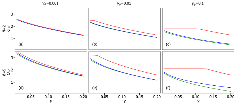
Here, we compare the previously derived bounds on the quantum capacity of the loss-dephasing channel for several dephasing rates , mean energies , and various loss rates . The results of this comparison are shown in Fig. 1. The lower bound is almost as tight as the lower bound obtained by optimizing over diagonal states, except for large and , i.e. . Both the lower bounds and the upper bounds are tight when the joint channel is dominated by either loss or dephasing, i.e., or . However, the bounds become looser when both and are large, as the joint channel deviates further from a degradable channel. Overall, both the lower and upper bounds increase as more energy is allowed for the bosonic mode. Another feature of the data processing upper bound is that, given , first increases as decreases and then saturates when . This feature appears because is, by definition, the minimum of the separate pure-loss and pure-dephasing channel capacities (see Eq. 27), which equals the latter (as a constant) when dephasing is dominant.
4 Numerically optimized error correction codes
Tailored encoding and decoding operations are required to faithfully transmit quantum information over a noisy channel . We use the entanglement fidelity [2] of the composite encoding-noise-decoding channel ( are identical message spaces available to and , respectively) as the figure of merit characterizing how well the information is preserved through . The optimal encoding and decoding strategy is thus given by
| (29) |
where is the entanglement fidelity of the composite channel, defined as the overlap between a maximally entangled state , and the state obtained after one part of is transmitted through :
| (30) |
where is a basis of and is the trace of a matrix representation of .
If is a bosonic system, we can modify this definition to handle energy-constrained encodings by defining
| (31) |
where is a maximally mixed state in .
Optimizing over either of the channels or while keeping the other fixed is a convex optimization problem. As such, this problem has a unique solution that is efficient to compute using semidefinite programming [17]. This insight leads to an intuitive biconvex optimization algorithm in which we iteratively find the optimal decoding given an updated encoding, and vice versa. However, the biconvex problem itself is not guaranteed to be convex. As a result, there might be cases where the algorithm does not converge or where the converged encoding depends on the chosen initial encoding.
Our numerical procedure optimizes the entanglement fidelity, but does not consider other important figures of merit. These include the performance of the encoding and decoding procedures themselves, or the difficulty in their experimental realization. In addition, the constraint on the average photon number fails to take into account the spread of the codes in Fock space. For example, the geometric distribution of GKP codes occupies a much larger number of energy levels than Poissonian-distributed cat codes with the same . Finally, increasing the entanglement fidelity of a code might not always increase its capacity to transmit information, as we will show in section 5.2.
For further details and results on the pure-loss channel, we refer to section 5 in Ref. [18]. In the next section, we expand on these results by adding dephasing noise. We find that the optimization algorithm consistently converges to unique encodings for various loss and dephasing rates.
4.1 Discussion of optimization results
To gain insight into the structure of numerically optimized qubit codes, we perform the optimization for various loss and dephasing rates. Since the loss-dephasing channel is covariant under rotations, rotating a code does not alter its performance. For the pure-dephasing channel, the optimized codes are also covariant under diagonal unitaries. Therefore, we regularize the codes accordingly after the optimization process (see Appendix C.1).
As long as the error rates are sufficiently high and the energy constraint sufficiently low, we consistently converge to the same optimal codes for a given triplet . The optimization results are shown in Fig. 2. Each plot represents an optimization result for a specific pair of loss and dephasing rates – that is, a local maximum of the entanglement fidelity. These local maxima are most likely also global maxima, since we observe that optimization runs with different randomly chosen initial codes converge to the same optimal code.
As we allow for higher or lower , the optimal value of the entanglement fidelity approaches one and the landscape becomes shallower, allowing for more local maxima with similar entanglement fidelities to appear. This causes the optimization result to depend on the initial state. Such parameter ranges are not considered and are represented in Fig. 2 by a shaded region.
A key takeaway from these results is that while numerically optimized codes for pure-loss or pure-dephasing channels saturate the mean energy constraint, this is not generally the case. Indeed, for the combined loss-dephasing channel with , the numerically optimized codes have a particular mean energy that does not vary when allowing higher energies.
5 Comparison with known codes
Various quantum error-correcting codes have been previously developed to protect against bosonic noise. For a short overview of GKP codes (which protect well against loss) [8], rotation codes [14] and numerical codes [19], see appendix D. Here, we show how these codes compare to the numerically optimized codes from this work.
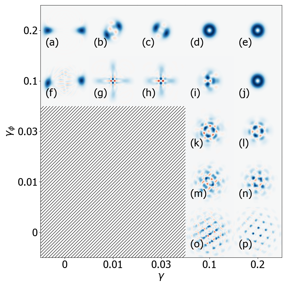
The optimization results depicted in Fig. 2 demonstrate the interplay between loss and dephasing and indicate the ranges of in which each of the GKP, cat and numerical codes excel [28]. The optimal codes for pure-loss noise (Figs. 2(o) and 2(p)) closely resemble hexagonal GKP codes, as previously observed by Noh et al. [6]. The optimal codes saturate the energy constraint, suggesting that GKP codes with more photons are better suited for dealing with loss.
In the case of pure-dephasing noise (Figs. 2(a) and 2(f)), we observe that two-legged cat codes and squeezed two-legged cat codes [29] provide optimal protection. Similarly to the GKP codes in the pure loss case, these codes saturate the energy constraint. This agrees with the known fact that the performance of two-legged cat codes improves as their mean energy increases [30, 31, 20, 32]. Squeezed two-legged cat codes have also been found to provide limited protection against photon loss in addition to dephasing [29].
Figs. 2(g) and 2(h) correspond to an encoding in which the code words are two-legged cats with opposite parities and orthogonal orientations in phase space. This encoding differs from the regular two-legged cat code, in which the orientation of the code words is identical. The separation of the code words in phase space offers protection against single-photon loss, besides the code’s suppression of dephasing errors (a similar observation was made in Ref. [33]). The modified two-legged cat code is also superior to the four-legged cat code [4] in that it also makes use of odd Fock states.
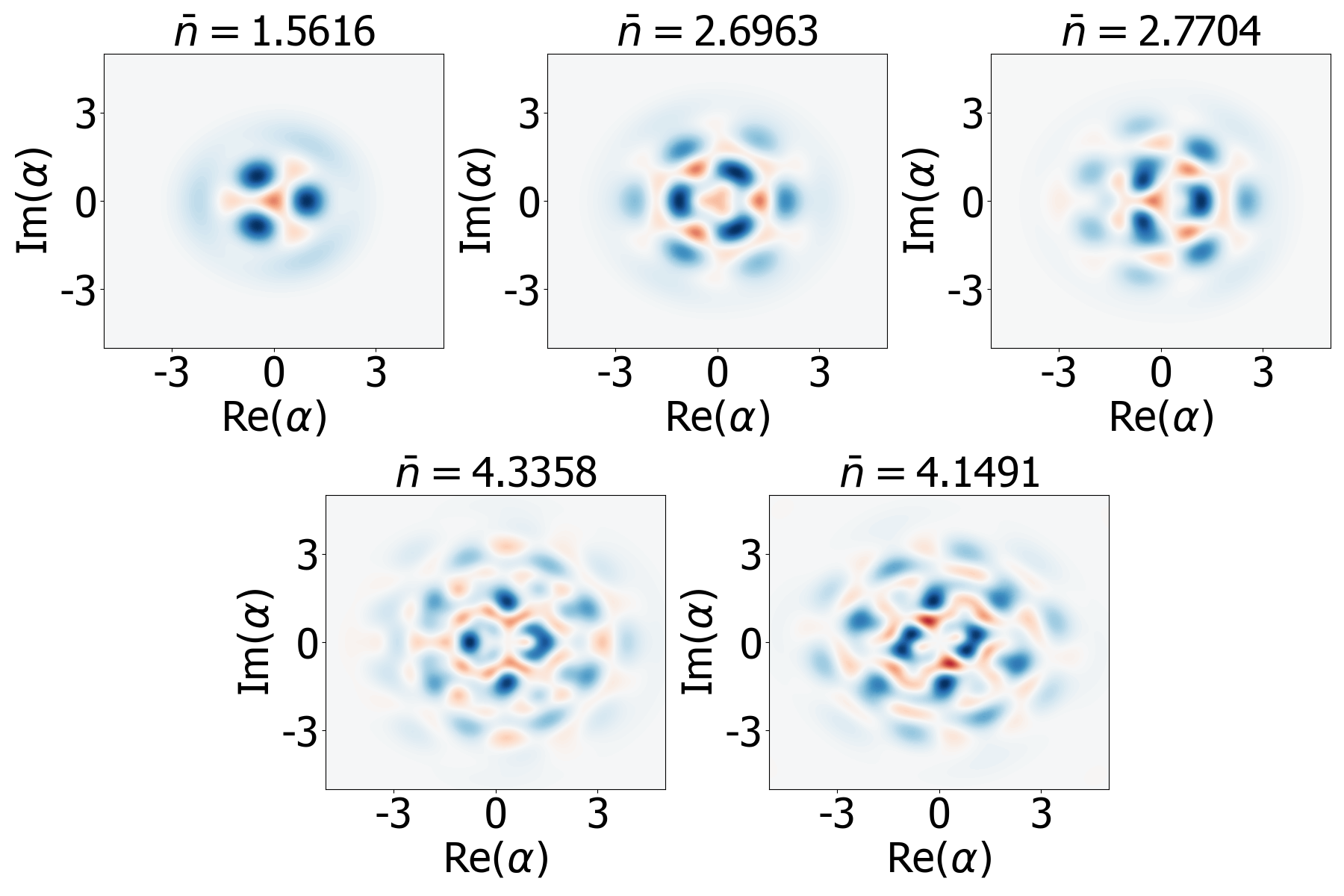
For all codes with nonzero dephasing and loss (i.e., or ), we observe that the energy constraint is not saturated (see Table 1 in Appendix C). Instead, these codes are characterized by varying optimal mean energies for different error rates. This situation is similar to the family of numerical codes [19], which consists of five different codes categorized by mean occupation number. However, unlike the numerical codes, our optimization process considers the error rates, resulting in different optimal codes for different . Out of those, (i),(k),(l) and (n) appear to be similar to some of the numerical codes (see Fig. 10 in the Appendix).
We also observe that certain codes have explicit rotational symmetry. For example, Figs. 2(k) and 2(l) are symmetric with respect to rotations by . However, these codes are not rotation codes [14]. Indeed, whereas the Fock-state distribution of the code words obeys -modularity, the remainders are not restricted to and as is the case for rotation codes (see Appendix D.2).
5.1 Entanglement fidelity
To evaluate the performance of the numerically optimized qubit codes, we compare their entanglement fidelities to those of the other major code families. Specifically, we use the following codes: hexagonal GKP codes as representatives of GKP codes, four-legged cat codes as representatives of rotation codes and finally, the five numerical codes presented in Ref. [5].
Within each of the code families, we choose the particular instance of the family that maximizes the entanglement fidelity, i.e.,
| (32) |
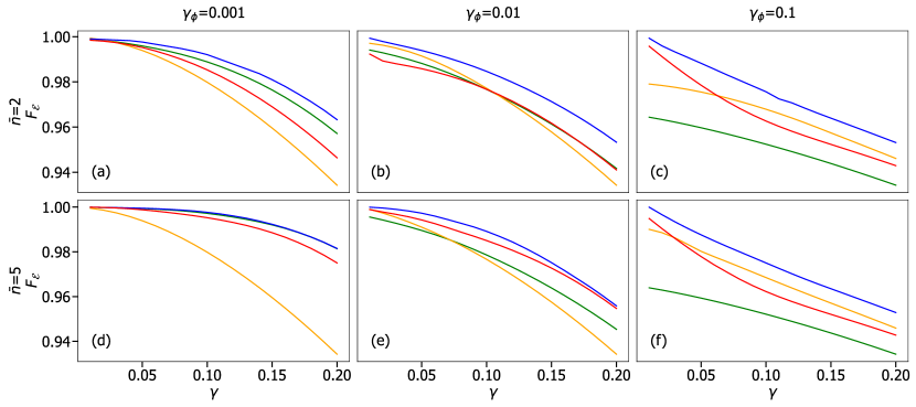
where is a four-legged cat, hexagonal GKP or numerical code qubit encoding with , and is an optimal decoding channel. The results of this comparison are shown in Fig. 3. In all cases, we find that the numerically optimized codes have the highest entanglement fidelity, as expected. For low dephasing rates (), hexagonal GKP codes offer the highest fidelity among the considered code families, while for high dephasing rates () cat codes perform better. The numerical codes offer good results for intermediate dephasing and sufficiently large .
5.2 Hashing bound
The bosonic codes derived in the previous section can be used to reliably communicate information over the loss-dephasing channel. In this section, we study how close the communication rate of each code comes to the quantum capacity of the channel . While the achievable communication rate of an encoding-noise-decoding channel is difficult to determine, it is bounded from below by the information-theoretic quantity known as the hashing bound , which we define below (see also corollary 21.2.1 and theorem 24.9.1 in [2] and theorem 3.1 in [34]).
Let (with and isomorphic) be an encoding-decoding pair for the channel , and let be a shared system isomorphic to . If is a maximally entangled state and , then the hashing bound of the combined channel is defined as
| (33) |
From the definition, we see that . Therefore, to meaningfully compare the communication rates of the codes to the theoretical limit , we generalize the qubit codes used earlier to qudit codes with dimension . Specifically, we use qudit codes obtained through biconvex optimization of the entanglement fidelity and known qudit code families, such as hexagonal GKP qudits (Eq. 48 in the Appendix) and 2-legged cat qudits (Eq. 50).
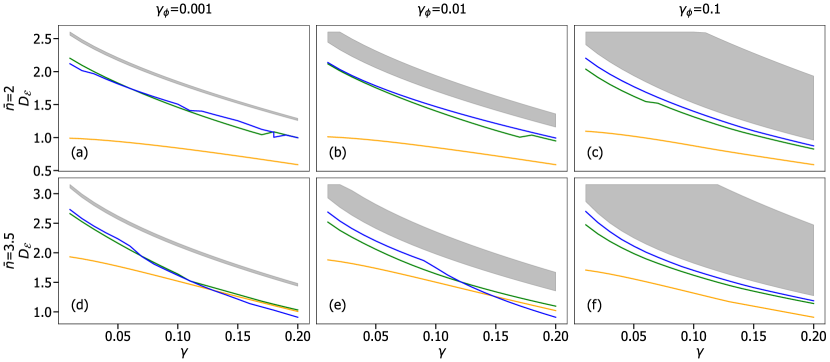
In Fig. 4, we plot the optimal hashing bounds
| (34) |
where are the qudit encodings for the respective code families with and mean energy , and are the optimal decodings.
The results indicate that the biconvex optimized codes and the GKP codes have very similar hashing bounds for all the considered parameter regimes. In addition, the hashing bounds are close to the previously derived lower bounds on the capacity of the loss-dephasing channel (Fig. 1). In some cases, we observe that the hashing bound of the hexagonal GKP code surpasses that of the biconvex optimized code. As previously observed in Ref. [5], optimizing the code for entanglement fidelity, as in our biconvex optimization scheme, does not necessarily imply an optimal hashing bound [35]. For example, introducing noise structure (e.g., biased noise) to at the cost of slightly reduced entanglement fidelity after decoding the inner bosonic code may result in a more efficient outer code using multiple copies of . This procedure might lead to a better hashing bound than the one associated with the bosonic code achieving maximal entanglement fidelity.
Finally, the relatively low hashing bound of the cat qudit code is due to the fact that for the code word has support on Fock states modulo (see section D.2 in the Appendix). Therefore, the mean energy of the code is greater than , limiting the hashing bound to . This implies that rotation codes are less compressed than other codes and require higher mean energy to provide the same capacity.
6 Conclusion
We presented a study of the bosonic loss-dephasing channel from multiple perspectives. We showed that, unlike the pure-loss (for ) and pure-dephasing channels, the loss-dephasing channel is not degradable, complicating the calculation of its capacity. To that end, we provided upper and lower bounds that prove to be tight for realistic values of . Next, we used a biconvex optimization scheme with an energy constraint to find numerically optimized codes for various loss and dephasing rates. We observed that two-legged cat codes are well suited for dephasing errors, while hexagonal GKP codes handle loss errors well. These two edge cases saturate the energy constraint. In contrast, when both loss and dephasing are present, the energy constraint is not saturated, and codes resembling numerical codes emerge. The optimization procedure reveals a phase space of codes that vary non-smoothly from GKP codes to cat codes. Finally, we connected the two perspectives using the hashing bound and showed that the single-mode biconvex optimized codes give rise to a satisfactory lower bound on the capacity. This implies that the optimized codes can be used for quantum communication schemes over the loss-dephasing channel with a relatively high communication rate.
The remaining open questions include a study of whether or not the channel is anti-degradable in a nontrivial error range (not just for ). We conjecture that the channel is not anti-degradable for and suggest that this may be proven using similar methods to the ones used here. Furthermore, good analytical bounds on the capacity remain to be found. One may also attempt to prove or contradict that for any , there exists a code with finite energy that maximizes the entanglement fidelity of and, if so, estimate its energy. Finally, this work does not consider the implementation of encoding, error correction, and decoding procedures. However, our results may be a good starting point for finding codes that are both experimentally feasible and perform well under realistic loss-dephasing noise.
Appendix A Quantum capacity of the pure-dephasing channel
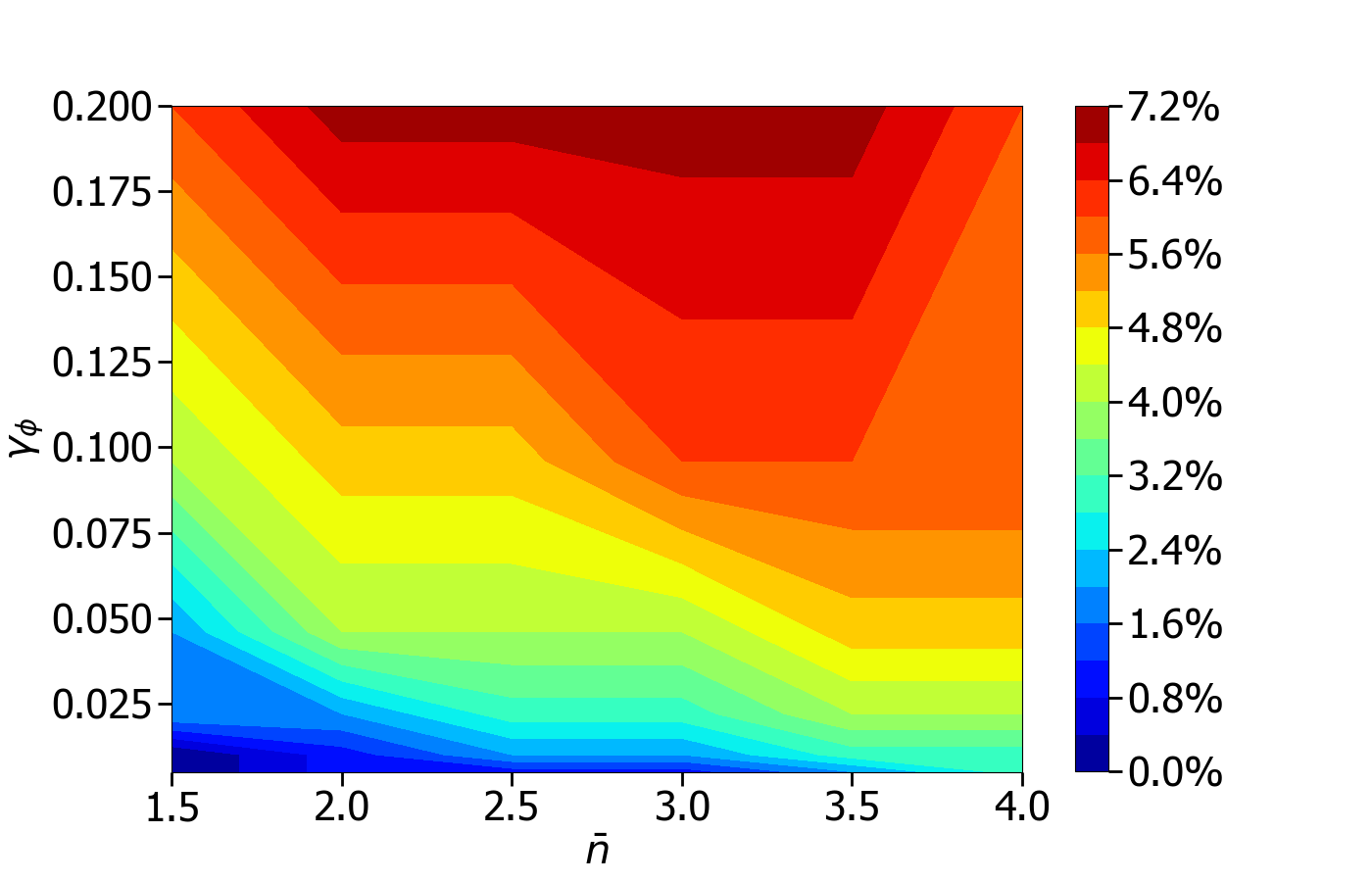
The energy-constrained quantum capacity of the dephasing channel can be evaluated using a numerical convex optimization procedure. The optimization can be limited to diagonal states due to the covariance of this channel with respect to phase-space rotations. We observe that the photon number distribution of the optimal input state resembles the Poissonian distribution of coherent states in shape, although it may have a different variance (see Fig. 5). Interestingly, for a large range of parameters, the coherent information of thermal states yields an excellent approximation to the quantum capacity (see Fig. 6).
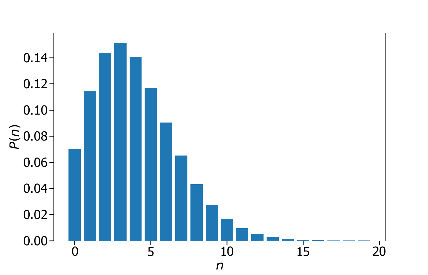
diagonal state for pure-dephasing noise with
and energy constraint .
Appendix B Non-degradability of the joint bosonic loss and dephasing channel
The aim of this appendix is to give a rigorous proof of the non-degradability of the loss-dephasing channel (Theorem Theorem) through a number of lemmas.
Lemma 1.
Let be the Stinespring dilation of a loss-dephasing channel . The channel is then given by
| (35) |
and the complementary channel is given by
| (36) |
Proof.
We start by calculating the state for any . We can combine the two identities
| (37) |
| (38) |
to determine that ,
| (39) |
We can now calculate the isometry on an arbitrary operator basis element :
| (40) |
Finally, tracing over the system forces , which yields the desired result for the complementary channel:
| (41) |
Similarly, tracing over the systems forces . Using the overlap between the coherent states , we obtain the expression for . ∎
Next, if we assume by contradiction that the loss-dephasing channel is degradable, then the degrading channel must assume the form presented in the following lemma.
Lemma 2.
If and is a degrading super-operator s.t. then must be the super-operator defined by
| (42) |
If , no such super-operator exists.
Proof.
We start by considering maximum photon loss, i.e., . In this case, the channel maps all states to the vacuum state. Since the complementary channel is not a constant channel, the degrading map does not exist.
Now, assume that . Then, for all integer ,
| (43) |
Using the previous lemma, we obtain
Using the abbreviated notation
the previous equation simplifies to . This allows one to invert the expression and obtain by induction on . Using the definition of we can rewrite as
| (44) |
Taking the adjoint of both sides of the equation gives us an expression for , so that Eq. 42 holds, as required. ∎
To prove that the channel is not degradable, we will evaluate the degradation super-operator on coherent states and show that it can map them to non-positive operators. We start with the following lemma:
Lemma 3.
For and , the map satisfies
| (45) |
where is a density matrix and is a dephasing super-operator with negative dephasing rate, i.e., it is not a channel.
Proof.
Plugging in the expression for from the previous lemma and using , we obtain
Taking we obtain,
Finally, note that , yielding the required result. ∎
The last lemma, which concludes the proof, shows that can be chosen s.t. is not a state. Hence is not a quantum channel.
Lemma 4.
If and then is not a quantum channel.
Proof.
It is sufficient to show that is not a positive map. Let s.t. , then for we have
| (46) |
since . This shows that . Therefore, is not a positive map and in particular, not a quantum channel. ∎
Appendix C Biconvex optimization of QEC codes for the loss-dephasing channel
We use biconvex optimization to find a local maximum in a complicated landscape defined by the entanglement fidelity. For the process to converge, it must run for many iterations. Moreover, the point to which it converges depends on the starting point.
For Fig. 2, we ran the optimization process for around 3000 iterations per plot. This process was repeated ten times with different randomized starting codes in each repetition. We then selected the optimal results for each pair of , while ensuring that the results from other repetitions yield similar codes. This consistency criterion indicates that the local optimum might also be a global optimum. This procedure works well when either or are large. However, when both parameters are small, the landscape becomes shallow. This makes it hard to converge to a single global maximum, leading to different optimization results for different starting codes. For this reason, we chose not to include the cases where both and are below .
As presented in the main text, the optimal codes do not always saturate the energy constraint (see Table 1).
| Mean energies | |||
|---|---|---|---|
| Index | |||
| a | 0.0 | 0.2 | 9.00 |
| b | 0.01 | 0.2 | 1.70 |
| c | 0.03 | 0.2 | 1.13 |
| d | 0.1 | 0.2 | 0.50 |
| e | 0.2 | 0.2 | 0.50 |
| f | 0.0 | 0.1 | 8.81 |
| g | 0.01 | 0.1 | 5.33 |
| h | 0.03 | 0.1 | 3.52 |
| i | 0.1 | 0.1 | 1.38 |
| j | 0.2 | 0.1 | 0.50 |
| k | 0.1 | 0.03 | 3.17 |
| l | 0.2 | 0.03 | 2.30 |
| m | 0.1 | 0.01 | 4.28 |
| n | 0.2 | 0.01 | 3.34 |
| o | 0.1 | 0.0 | 8.38 |
| p | 0.2 | 0.0 | 9.00 |
In some of the cases where either or , the mean energy comes close to the constraint but does not saturate it. This is most likely due to numerical limitations of the optimization and the fact that we used a limited number of energy levels ().
C.1 Regularization process for comparison of numerically optimal codes
The loss-dephasing channel is invariant under phase-space rotations, which causes optimization results with different starting points to be similar up to rotations. To tackle this, we regularize the codes by concatenating them with and imposing a condition that a particular off-diagonal element in the density matrix of the maximally mixed state of the resulting code is positive. Similarly, the pure-loss channel is invariant under rotations, and the same regularization is applied there. The pure-dephasing channel, however, is also invariant under diagonal unitaries. Therefore, in that case we regularize the code by concatenating it with , where is a diagonal matrix with real entries. These entries are chosen such that a single off-diagonal element in each row of the density matrix of the maximally mixed state becomes positive. This results in codes with plots such as (a) and (f) in Fig. 2.
C.2 Optimization results for the pure-loss channel with low energy constraints.
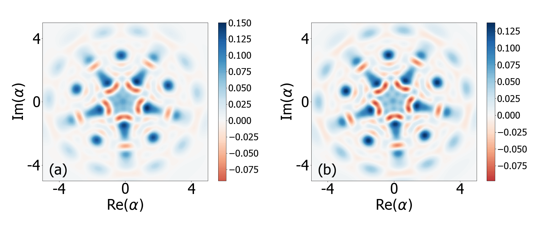
Hexagonal GKP codes emerge as optimal codes for the pure-loss channel if the energy constraint is chosen to be sufficiently high. However, if the energy constraint is low (e.g., or ), and if the loss rate is sufficiently high (e.g., ), the optimization result is a code with five-fold rotation symmetry (see Fig. 7). A potential insight as to why this might be the case is that, like the GKP code, we can use a tiling to protect against random shifts. However, due to the energy constraint, the tiling is not shift-invariant and distorts as we move away from the origin. A hyperbolic plane may be a good model for this phenomenon, and this plane can be tiled by pentagrams, as we observe here.
Appendix D Overview of bosonic error correction codes
D.1 GKP codes
GKP codes [8] are lattice codes that are particularly well suited for handling phase-space displacements and bosonic loss noise [5]. GKP codes can be either single-mode (as used in this work) or defined using modes. If they are -dimensional, the code words can be seen as superpositions of infinitely many -mode coherent states centered around points of a non-degenerate -dimensional lattice in phase space. As such, they have infinite energy. A common way to modify the code to have finite energy, is to multiply the coherent states by weights from a Gaussian envelope, with narrower envelopes corresponding to lower mean energy of the code.
For example, if is a matrix with columns that span a lattice in a -dimensional phase space with coordinates (), we can define the code words of a finite-energy GKP qudit based on as [5]
| (47) |
where are -mode displacements.
In particular, for the hexagonal GKP qudits () referred to in the main text, the lattice is given by
| (48) |
GKP codes can be seen as stabilizer codes over commuting displacements . Therefore, not any lattice can be used to define a valid GKP code. In the single-mode case, for example, this requirement translates to , so that a GKP code with square lattice will have and . The condition on for is more involved and is discussed, for example, in section 2.4.3 of Ref. [7].
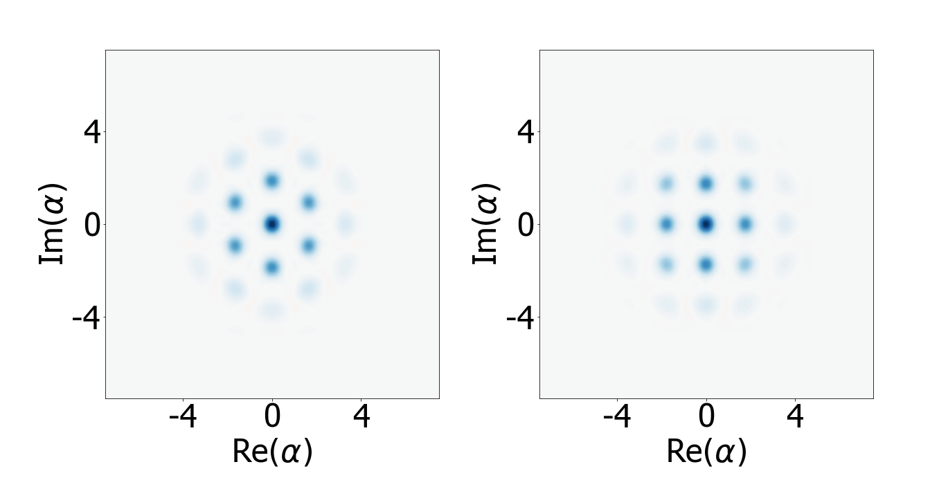
The performance of a GKP code depends on the lattice that defines it, with lattices that have a higher ratio of sphere packing (ratio between the volume of the largest -sphere that can inhabit the Voronoi cell and the volume of the cell itself) performing better. This means, for example, that a single-mode GKP code defined by a hexagonal lattice will perform better than a code defined by a square lattice (see section 4 in Ref. [18]). Both codes are presented in Fig. 8.
Ref. [18] also shows that GKP codes perform well for bosonic loss in two crucial ways. The first is that infinite-energy multi-mode GKP codes achieve a quantum communication rate that is offset by up to from the capacity of the channel in the limit where the number of modes goes to infinity. This feature holds for any loss rate between and . The second advantage of GKP codes is that the biconvex optimization process described earlier usually converges to a state resembling a hexagonal GKP state with finite energy if only loss is present. However, as discussed in appendix C, for certain energy constraints it can also converge consistently to other codes. For example, a code with five-fold symmetry can emerge, probably due to a requirement to tile a bounded section of phase space.
D.2 Rotation codes
A single-mode bosonic qudit encoding with code words is a called a rotation code [14] with symmetry if the code words are invariant under the rotation and if the rotation acts as a logical on the qudit:
| (49) |
Cat codes and binomial codes are examples of rotation codes (Fig. 9). Ref. [14] provides a scheme for performing encoding, decoding and gates on such codes based on controlled rotation gates and phase measurements.
The logical code words of a -legged cat qudit, as referred to in the main text, are defined by
| (50) |
where is a coherent state with .
Since the code word of a rotation code is supported by Fock states that are modulo , rotation codes provide protection (or at least detection) against up to photon loss events. If the code is also a number-phase code, that is, the phases of the code words in the conjugate basis are well localized (modulo a rotation), then the phases of the code words are also well separated. This property protects the code against dephasing errors. Number-phase codes are similar to GKP codes in that, whereas the former use photon number-phase duality to define the code, the latter rely on position-momentum duality.
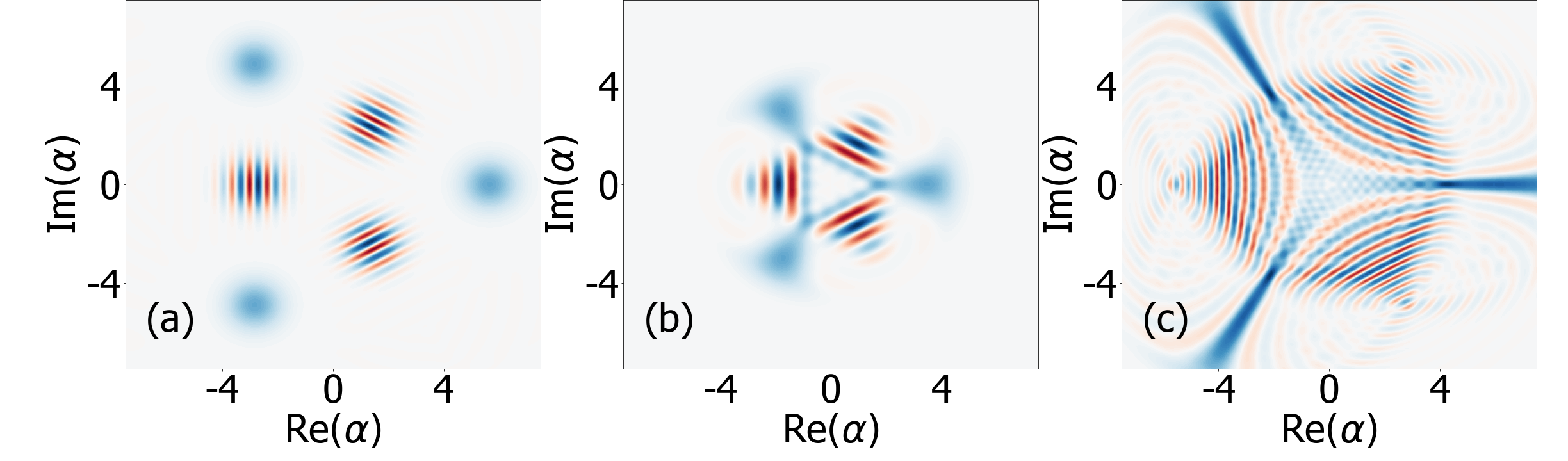
In our numerical optimizations, we found that for pure dephasing (), we converge to rotation codes with code words that resemble squeezed coherent states. However, when adding loss, we sometimes converge to codes that are invariant under rotations but are not rotation codes. Indeed, the condition for the logical operator to be a rotation may be too restrictive. Examples of such codes include GKP codes and the numerically optimized codes plotted in Fig. 7 and in Figs. 2(k) and 2(l). More precisely, a qudit code has rotation symmetry (as opposed to being a rotation code) if its maximally mixed state commutes with the rotation .
Alternatively, the code words can be chosen to have a defined modularity mod :
Claim 1.
If a qudit code has rotation symmetry and there exist integers that are all different modulo s.t. for all , then we can choose different code words s.t. is supported on .
Proof.
The operators and commute, and both are diagonalizable. Therefore, they are simultaneously diagonalizable and we can find eigenstates of that are also eigenstates of . Since the eigenvalues of are , we obtain eigenstates of with eigenvalue . Because the states are also eigenstates of , they each lie in for some integer . However, since overlaps with for all and they are all different modulo , the ’s must be different. Therefore, can be chosen to lie in . ∎
D.3 Numerical codes
Numerical codes, first introduced in Ref. [19], emerge from a different numerical optimization scheme than the one used here. For example, these codes include the code
The cost function of the optimization process is a function of coefficients of the quantum error correction matrix, which is constructed from a finite set of noise operators. In the original article [19] and in Ref. [5], the noise operators were taken to be . The codes are obtained from local minima of the cost function with a penalty on average energy. Five codes were identified in this manner. We plot the Wigner distributions of their maximally mixed states in Fig. 10. Note that a different set of noise operators would result in different numerically optimal codes. In particular, the errors are given the same weights, which is not necessarily desired when considering specific error rates. For example, if the loss rate is low, we should assign a larger weight to . If the loss rate is high, we should assign a larger weight to , and perhaps even consider higher powers of .
Since the quantum error correction matrix consists of elements of the form with in our case, numerical codes are expected to perform well under loss (of up to two photons) and dephasing (with its first Kraus operator ). Indeed, there is a large parameter range for which our biconvex optimization scheme outputs codes similar to numerical codes (e.g., Fig. 2(f)).
References
- [1] Peter W. Shor “Scheme for reducing decoherence in quantum computer memory” In Physical Review A 52.4 American Physical Society, 1995, pp. R2493 DOI: 10.1103/PhysRevA.52.R2493
- [2] Mark M. Wilde “Quantum information theory” In Quantum Information Theory Cambridge University Press, 2013 DOI: 10.1017/CBO9781139525343
- [3] Seth Lloyd “Capacity of the noisy quantum channel” In Physical Review A 55.3 American Physical Society, 1997, pp. 1613 DOI: 10.1103/PhysRevA.55.1613
- [4] Nissim Ofek et al. “Extending the lifetime of a quantum bit with error correction in superconducting circuits” In Nature 536.7617 Nature Publishing Group, 2016, pp. 441–445 DOI: 10.1038/nature18949
- [5] Victor V. Albert et al. “Performance and structure of single-mode bosonic codes” In Physical Review A 97.3 American Physical Society, 2018, pp. 032346 DOI: 10.1103/PhysRevA.97.032346
- [6] Kyungjoo Noh and Christopher Chamberland “Fault-tolerant bosonic quantum error correction with the surface-Gottesman-Kitaev-Preskill code” In Physical Review A 101.1 American Physical Society, 2020, pp. 012316 DOI: 10.1103/PhysRevA.101.012316
- [7] Kyungjoo Noh “Quantum Computation and Communication in Bosonic Systems”, 2020
- [8] Daniel Gottesman, Alexei Kitaev and John Preskill “Encoding a qubit in an oscillator” In Physical Review A 64.1 American Physical Society, 2001, pp. 012310 DOI: 10.1103/PhysRevA.64.012310
- [9] P. Campagne-Ibarcq et al. “Quantum error correction of a qubit encoded in grid states of an oscillator” In Nature 584.7821 Nature Research, 2020, pp. 368–372 DOI: 10.1038/s41586-020-2603-3
- [10] A. Romanenko et al. “Three-Dimensional Superconducting Resonators at T <20mK with Photon Lifetimes up to =2 s” In Physical Review Applied 13.3 American Physical Society, 2020, pp. 34032 DOI: 10.1103/PhysRevApplied.13.034032
- [11] Matthew Reagor et al. “Quantum memory with millisecond coherence in circuit QED” In Physical Review B 94.1 American Physical Society, 2016, pp. 014506 DOI: 10.1103/PhysRevB.94.014506
- [12] S. Rosenblum et al. “Fault-tolerant detection of a quantum error” In Science 361.6399 American Association for the Advancement of Science, 2018, pp. 266–270 DOI: 10.1126/science.aat3996
- [13] A.. Sears et al. “Photon shot noise dephasing in the strong-dispersive limit of circuit QED” In Physical Review B 86.18 American Physical Society, 2012, pp. 180504 DOI: 10.1103/PhysRevB.86.180504
- [14] Arne L. Grimsmo, Joshua Combes and Ben Q. Baragiola “Quantum Computing with Rotation-Symmetric Bosonic Codes” In Physical Review X 10.1 American Physical Society, 2020, pp. 011058 DOI: 10.1103/PhysRevX.10.011058
- [15] Yingkai Ouyang and Earl T. Campbell “Trade-Offs on Number and Phase Shift Resilience in Bosonic Quantum Codes” In IEEE Transactions on Information Theory 67.10 Institute of ElectricalElectronics Engineers Inc., 2021, pp. 6644–6652 DOI: 10.1109/TIT.2021.3102873
- [16] Felix Leditzky, Debbie Leung and Graeme Smith “Dephrasure Channel and Superadditivity of Coherent Information” In Physical Review Letters 121.16 American Physical Society, 2018, pp. 160501 DOI: 10.1103/PHYSREVLETT.121.160501
- [17] Robert L. Kosut and Daniel A. Lidar “Quantum error correction via convex optimization” In Quantum Information Processing 8.5 Springer, 2009, pp. 443–459 DOI: 10.1007/S11128-009-0120-2
- [18] Kyungjoo Noh, Victor V. Albert and Liang Jiang “Quantum Capacity Bounds of Gaussian Thermal Loss Channels and Achievable Rates with Gottesman-Kitaev-Preskill Codes” In IEEE Transactions on Information Theory 65.4 Institute of ElectricalElectronics Engineers Inc., 2019, pp. 2563–2582 DOI: 10.1109/TIT.2018.2873764
- [19] Marios H. Michael et al. “New class of quantum error-correcting codes for a bosonic mode” In Physical Review X 6.3 American Physical Society, 2016, pp. 031006 DOI: 10.1103/PhysRevX.6.031006
- [20] Mazyar Mirrahimi et al. “Dynamically protected cat-qubits: A new paradigm for universal quantum computation” In New Journal of Physics 16.4 Institute of Physics Publishing, 2014, pp. 045014 DOI: 10.1088/1367-2630/16/4/045014
- [21] Amir Arqand, Laleh Memarzadeh and Stefano Mancini “Quantum capacity of a bosonic dephasing channel” In Physical Review A 102.4, 2020, pp. 42413 DOI: 10.1103/PhysRevA.102.042413
- [22] Andreas Winter “Energy-constrained diamond norm with applications to the uniform continuity of continuous variable channel capacities” In arXiv:1712.10267 [quant-ph], 2017 DOI: 10.48550/arXiv.1712.10267
- [23] Michael M. Wolf, David Pérez-García and Geza Giedke “Quantum capacities of bosonic channels” In Physical Review Letters 98.13 American Physical Society, 2007, pp. 130501 DOI: 10.1103/PHYSREVLETT.98.130501
- [24] Christian Weedbrook et al. “Gaussian quantum information” In Reviews of Modern Physics 84.2 American Physical Society, 2012, pp. 621–669 DOI: 10.1103/RevModPhys.84.621
- [25] Mark M. Wilde and Haoyu Qi “Energy-constrained private and quantum capacities of quantum channels” In IEEE Transactions on Information Theory 64.12 Institute of ElectricalElectronics Engineers Inc., 2018, pp. 7802–7827 DOI: 10.1109/TIT.2018.2854766
- [26] Ludovico Lami and Mark M. Wilde “Exact solution for the quantum and private capacities of bosonic dephasing channels” In arXiv:2205.05736 [quant-ph], 2022 DOI: 10.48550/arxiv.2205.05736
- [27] Vikesh Siddhu and Robert B. Griffiths “Positivity and nonadditivity of quantum capacities using generalized erasure channels” In IEEE Transactions on Information Theory 67.7 Institute of ElectricalElectronics Engineers Inc., 2021, pp. 4533–4545 DOI: 10.1109/TIT.2021.3080819
- [28] Atharv Joshi, Kyungjoo Noh and Yvonne Y Gao “Quantum information processing with bosonic qubits in circuit QED” In Quantum Science and Technology 6.3 IOP Publishing, 2021, pp. 033001 DOI: 10.1088/2058-9565/ABE989
- [29] David S. Schlegel, Fabrizio Minganti and Vincenzo Savona “Quantum error correction using squeezed Schrödinger cat states” In arXiv:2201.02570 [quant-ph], 2022 DOI: 10.48550/arXiv.2201.02570
- [30] A. Grimm et al. “Stabilization and operation of a Kerr-cat qubit” In Nature 584.7820 Nature Publishing Group, 2020, pp. 205–209 DOI: 10.1038/s41586-020-2587-z
- [31] C. Berdou et al. “One hundred second bit-flip time in a two-photon dissipative oscillator” In arXiv:2204.09128 [quant-ph], 2022 DOI: 10.48550/arxiv.2204.09128
- [32] Raphaël Lescanne et al. “Exponential suppression of bit-flips in a qubit encoded in an oscillator” In Nature Physics 16.5 Nature Research, 2020, pp. 509–513 DOI: 10.1038/s41567-020-0824-x
- [33] Linshu Li et al. “Phase-engineered bosonic quantum codes” In Physical Review A 103.6 American Physical Society, 2021, pp. 062427 DOI: 10.1103/PhysRevA.103.062427
- [34] Igor Devetak and Andreas Winter “Distillation of secret key and entanglement from quantum states” In Proceedings of the Royal Society A: Mathematical, Physical and Engineering Sciences 461.2053 Royal Society, 2003, pp. 207–235 DOI: 10.1098/rspa.2004.1372
- [35] Johannes Bausch and Felix Leditzky “Quantum Codes from Neural Networks” In New Journal of Physics 22.2 IOP Publishing, 2018, pp. 023005 DOI: 10.1088/1367-2630/ab6cdd
