A nonparametric regression alternative to empirical Bayes approaches to simultaneous estimation

Abstract

The simultaneous estimation of multiple unknown parameters lies at heart of a broad class of important problems across science and technology. Currently, the state-of-the-art performance in the such problems is achieved by nonparametric empirical Bayes methods. However, these approaches still suffer from two major issues. First, they solve a frequentist problem but do so by following Bayesian reasoning, posing a philosophical dilemma that has contributed to somewhat uneasy attitudes toward empirical Bayes methodology. Second, their computation relies on certain density estimates that become extremely unreliable in some complex simultaneous estimation problems. In this paper, we study these issues in the context of the canonical Gaussian sequence problem. We propose an entirely frequentist alternative to nonparametric empirical Bayes methods by establishing a connection between simultaneous estimation and penalized nonparametric regression. We use flexible regularization strategies, such as shape constraints, to derive accurate estimators without appealing to Bayesian arguments. We prove that our estimators achieve asymptotically optimal regret and show that they are competitive with or can outperform nonparametric empirical Bayes methods in simulations and an analysis of spatially resolved gene expression data.

1 Introduction

We consider the problem of simultaneously estimating multiple unknown parameters of interest. A canonical problem is to estimate a vector $(\theta_{1},\dots,\theta_{n})^{\top}$ given independent observations $X_{i}\sim N(\theta_{i},\sigma^{2})$ for $i=1,\ldots,n$, where $\sigma>0$ is known. This Gaussian sequence problem (Johnstone, 2019) is a foundational model in theoretical statistics because it captures the core issues at the heart of a broad class of important problems across science and technology. For example, in large-scale A/B testing, a large number of randomized experiments are conducted to evaluate the effects of multiple types of treatments on multiple types of metrics, and a common goal is to simultaneously estimate every treatment effect (Guo et al., 2020; Ignatiadis et al., 2021; Muralidharan, 2010). In genomics it is common to profile tens of thousands of genomic features, and a frequent goal is to simultaneously estimate the association between each feature and some phenotype (Love et al., 2014; Robinson et al., 2010; Smyth, 2004). Other domains where similar issues arise include small area estimation (Rao and Molina, 2015), econometrics (Koenker and Gu, 2023), and large-scale inference (Efron, 2012). As the scale, complexity, and number of unknown parameters in moden experiments has exploded, understanding simultaneous estimation has become increasingly important.

The key statistical feature of simultaneous estimation problems is that the most natural approach, where each parameter is estimated separately, can be suboptimal. In the Gaussian sequence problem, this corresponds to estimating each $\theta_{i}$ using $X_{i}$, and early results (Robbins, 1951; Stein, 1956) found that this estimator is inadmissible under squared error loss when $n\geq 3$. The overall lesson of this and subsequent work is that estimating $\theta_{i}$ by including information from the other indices $j\neq i$, even though they may seem unrelated, can improve overall accuracy (Fourdrinier et al., 2018; Johnstone, 2019). These estimators are often called shrinkage estimators, because early estimators such as one by James and Stein (1961) dominated the naive estimators $X_{i}$ by shrinking them toward zero. These discoveries came as a major surprise and set off a long and rich line of research to better understand shrinkage and to develop more accurate estimators. Our goal in this paper is to further enrich our understanding of this phenomenon.

The modern approach to simultaneous estimation is to use empirical Bayes methods (Efron, 2014, 2019; Zhang, 2003). These methods are Bayesian in the sense that they pretend that the unknown parameters are random samples from some prior distribution, then estimate the parameters using posterior means or medians. They are “empirical” Bayesian because the prior is estimated using the observed data, since it is generally unknown. In the Gaussian sequence problem, the empirical Bayes approach pretends that the true means $\theta_{i}$ are random with some prior distribution $G$ and estimates $\theta_{i}$ using its posterior mean

$$E(\theta\mid X=X_{i})=\frac{\int_{-\infty}^{\infty}t\phi_{\sigma}(t-X_{i})dG(t)}{\int_{-\infty}^{\infty}\phi_{\sigma}(t-X_{i})dG(t)}=X_{i}+\sigma^{2}\frac{f_{G}^{\prime}(X_{i})}{f_{G}(X_{i})},$$ (1)

where $\phi_{\sigma}(\cdot)$ denotes the density function of a $N(0,\sigma^{2})$ random variable and $f_{G}(x)$ denotes what the marginal density of the $X_{i}$ would be if the $\theta_{i}$ indeed were random. The second equality is often called Tweedie’s formula (Efron, 2011). Since $G$ is unknown, (1) cannot be calculated, so the observed data are used to construct plug-in estimates of $E(\theta\mid X=x)$. Efron (2014) divides empirical Bayes methods into two classes: $f$-modeling and $g$-modeling, depending on whether the marginal $f_{G}$ or prior $G$ is substituted into (1), respectively. For example, Efron and Morris (1973) showed that the shrinkage estimator of James and Stein (1961) can be recovered as a $g$-modeling procedure under a normal assumption on the prior.

Currently, the state-of-the-art performance in the Gaussian sequence problem is achieved by nonparametric empirical Bayes methods. Brown and Greenshtein (2009) proposed an $f$-modeling procedure that estimates $f_{G}$ using a kernel density estimator and Jiang and Zhang (2009) proposed a $g$-modeling procedure that estimates $G$ using nonparametric maximum likelihood (Kiefer and Wolfowitz, 1956),which Koenker and Mizera (2014) showed can be efficiently calculated using modern convex optimization techniques. These methods are asymptotically optimal under squared-error risk, in the following sense. Robbins (1951) formulated the Gaussian sequence problem as finding a decision rule $\delta(X_{1},\ldots,X_{n})$ that has a small mean squared error $E\sum_{i}\{\theta_{i}-\delta_{i}(X_{1},\ldots,X_{n})\}^{2}$. He referred to this as an example of a compound decision problem, as multiple decisions need to be made to estimate multiple $\theta_{i}$. He focused on the class of so-called separable estimators, where $\delta_{i}(X_{1},\ldots,X_{n})=d(X_{i})$ for some fixed function $d$, and showed that

$$d^{*}(x)=\frac{\sum_{i=1}^{n}\theta_{i}\phi_{\sigma}(\theta_{i}-x)}{\sum_{i=1}^{n}\phi_{\sigma}(\theta_{i}-x)}.$$ (2)

minimizes mean squared error over all separable estimators. The estimator $\hat{d}_{JZ}(x)$ of Jiang and Zhang (2009) is asymptotically optimal in that

$$\limsup_{n\rightarrow\infty}\frac{E\sum_{i}[\{\theta_{i}-\hat{d}_{JZ}(X_{i})\}^{2}]}{E\sum_{i}[\{\theta_{i}-d^{*}(X_{i})\}^{2}]}=1$$ (3)

for any $(\theta_{1},\ldots,\theta_{n})^{\top}$ under mild conditions, and the estimator $\hat{d}_{BG}(x)$ of Brown and Greenshtein (2009) enjoys a similar property.

However, despite their excellent performance, nonparametric empirical Bayes approaches still suffer from two major issues. The first is philosophical: these methods solve a frequentist problem, but they do so by following Bayesian reasoning. They have good frequentist properties, but this “philosophical identity problem” has nevertheless contributed to somewhat uneasy attitudes toward empirical Bayesian methods that may limit their uptake (Efron, 2019). The second issue is practical and emerges in recent work that has started to consider how nonparametric empirical Bayes approaches can be applied to more complex problems. These include estimating multidimensional $\theta_{i}$ (Saha and Guntuboyina, 2020; Soloff et al., 2021), covariance matrix estimation (Xin and Zhao, 2022), and regression (Kim et al., 2022; Wang and Zhao, 2021). For example, Wang and Zhao (2021) studied the multivariate regression setting $Y_{ik}=X_{i}^{\top}\beta_{k}^{\star}+\epsilon_{ik}\sim N(0,\tau_{k}^{2})$ for outcomes $k=1,\ldots,K$. Their nonparametric empirical Bayes method pretends that $\beta_{k}^{\star}\sim G(b)$ and estimates $G(b)$ by maximizing the marginal likelihood:

$$\hat{G}(b)=\arg\max_{G}\prod_{k=1}^{K}\int\frac{1}{\{2\pi(\tau^{2}/n)\}^{1/2}}\exp\left\{-\frac{n}{2\tau^{2}}(\bar{Y}_{k}-\bar{X}^{\top}b)^{2}\right\}dG(b),$$

where $n$ is the sample size, $\bar{Y}_{k}$ and $\bar{X}$ are the sample means of the $Y_{ik}$ and $X_{i}$. Koenker and Mizera (2014) noted that an approximation to $\hat{G}(b)$ can be conveniently obtained by maximizing over all discrete distributions supported on a pre-specified grid of points, which is a convex optimization problem. However, when $n$ is large, the density in the integrand can be extremely small at most of the grid points, which caused problems even when using modern optimization software such as MOSEK.

In this paper we study these issues using the canonical Gaussian sequence problem. In this setting we model the low density issue described above by generating $X_{i}\sim N(\theta_{i},\sigma^{2})$ with low noise. When $\sigma^{2}$ is small, the densities that arise in these problems can suffer from the same numerical issues as those encountered in the more complex simultaneous estimation problems. This is further discussed in Section 5.3 and may account for the poor performance of $\hat{d}_{JZ}(x)$ and $\hat{d}_{BG}(x)$ in simulations.

To avoid these issues, we propose a new, alternative approach to the Gaussian sequence problem. First, our approach is purely frequentist and is based on the compound decision theoretic formulation of Robbins (1951). We establish a connection between simultaneous estimation and nonparametric regression and adopt an empirical risk minimization strategy that converts the problem into a penalized least-squares problem. We use flexible regularization strategies, such as shape constraints, to derive accurate estimators without appealing to Bayesian arguments. Second, our new approach can still achieve a similar accuracy as nonparametric empirical Bayes methods. We prove that our estimators achieve asymptotically optimal regret. Finally, our approach is robust to small $\sigma^{2}$. We show in simulations that the performances of our estimators are comparable to those of $\hat{d}_{BG}(x)$ and $\hat{d}_{JZ}(x)$ in high-noise settings and superior in low-noise settings. We also apply these methods to denoise spatially resolved gene expression data and show that our proposed procedures achieve the best results. In the future, we hope that generalizations of our approach can lead to novel estimators with distinct advantages in more complex simultaneous estimation problems.

2 A Penalized Regression Framework

Our framework is motivated by the observation by Stigler (1990) that finding a good estimator of the oracle separable estimator $d^{*}(x)$ (2) closely resembles least-squares regression. Specifically, if we had the oracle coordinate pairs $(X_{i},\theta_{i})$, we could model and estimate $d^{*}(x)$ by minimizing the oracle loss

$$R_{n}(d)=n^{-1}\sum_{i=1}^{n}\{\theta_{i}-d(X_{i})\}^{2}$$ (4)

using ordinary least squares. Minimizing $R_{n}(d)$ is not possible because $\theta_{i}$ are unknown. Stigler (1990) solved this problem for the class of linear models $d_{a,b}(x)=a+bx$. He first found the oracle linear model assuming $\theta_{i}$ were known and then developed method-of-moments-type estimates of those coefficients. Interesting, this essentially gave Stein-type shrinkage estimators and provided a new interpretation of shrinkage. However, his method-of-moments approach is restricted to the linear class $d_{a,b}(x)$, so this strategy cannot give estimators as accurate as the nonlinear ones produced by nonparametric empirical Bayes methods.

Our main insight is to combine Stigler’s regression perspective with empirical risk minimization ideas. Instead of deriving the oracle minimizer of $R_{n}(d)$ and then estimating it, as in Stigler (1990), our approach is to estimate $R_{n}(d)$ and then minimize the empirical loss. This strategy allows us to take advantage of many useful tools developed in the nonparametric regression and empirical risk minimization literatures, such as the easy implementation of shape constraints and a well-established set of techniques for theoretical analysis (van der Vaart and Wellner, 1996; Wainwright, 2019).

Our main task is therefore to develop a computable estimate of $R_{n}(d)$ that can be directly minimized. A natural approach is to plug in $X_{i}$ for each $\theta_{i}$ to produce the loss estimate $\hat{R}_{\text{naive}}(d)=n^{-1}\sum_{i=1}^{n}\{X_{i}-d(X_{i})\}^{2}$, but without further regularization $\hat{R}_{\text{naive}}(d)$ can be exactly minimized by the identity function $d(x)=x$. This is a problem because the identity function corresponds to the naive estimator, so we know that the minimizer of $\hat{R}_{\text{naive}}(d)$ will never produce asymptotically optimal estimators.

Instead, we use Stein’s lemma (Stein, 1981) to develop an unbiased estimate of $R_{n}(d)$ for a large class of $d(x)$. If $d(x)$ is an absolutely continuous function, then

$$R(d;\theta) =\frac{1}{n}\sum_{i=1}^{n}E\{\theta_{i}-d(X_{i})\}^{2}$$

$$=\frac{1}{n}\sum_{i=1}^{n}E\{X_{i}-d(X_{i})\}^{2}+\frac{2}{n}\sum_{i=1}^{n}E\{(X_{i}-\theta_{i})d(X_{i})\}-\sigma^{2}$$

$$=\frac{1}{n}\sum_{i=1}^{n}E\{X_{i}-d(X_{i})\}^{2}+\frac{2\sigma^{2}}{n}\sum_{i=1}^{n}E\{d^{\prime}(X_{i})\}-\sigma^{2}.$$ (5)

We note that it is actually sufficient for $d(x)$ to be weakly differentiable; however, we will stick to absolute continuity for consistency with our later discussion. With this risk decomposition, an unbiased estimate of $R_{n}(d)$ is:

$$\hat{R}_{1}(d)=\frac{1}{n}\sum_{i=1}^{n}\{X_{i}-d(X_{i})\}^{2}+\frac{2\sigma^{2}}{n}\sum_{i=1}^{n}d^{\prime}(X_{i})-\sigma^{2}.$$ (6)

In our regresson framework, the risk estimate (6), often called Stein’s unbiased risk estimate (SURE), is readily interpreted as a penalized least-squares loss. We note that in contrast to most penalized least-squares regression problems, $\hat{R}_{1}(d)$ does not have a tuning parameter that governs the trade-off between the goodness-of-fit and parsimony of the fitted function.

The penalized loss (6) has interesting connections to existing methodology. First, since Stein’s lemma is used to compute the covariance between $X_{i}$ and $d(X_{i})$, the penalty term can be thought of as a covariance penalty similar to Akaike’s information criterion and Mallow’s $C_{p}$ criterion (Efron, 2004; Akaike, 1973; Mallows, 1973). In contrast to most uses of these information criteria, here we use the covariance penalty in the fitting procedure rather than for model evaluation after fitting. Second, if we restrict $d(x)$ to be monotone non-decreasing, the penalty term can be seen as an $\ell_{1}$-type penalty; this suggests many connections to existing $\ell_{1}$-penalized least-squared regression problems. For example, if we parameterize $d(x)$ to be a continuous, piecewise linear function with knots at each $X_{i}$, then (6) becomes an irregularly spaced, degree-one trend-filter (Tibshirani, 2014b). Third, for any monotone non-decreasing $d(x)$, the penalty can be interpreted as a weighted total variation penalty. To see this, let $F_{n}(t)$ denote the empirical distribution of $X_{i}$. Then $n^{-1}\sum_{i=1}^{n}d^{\prime}(X_{i})=\int_{-\infty}^{\infty}|d^{\prime}(t)|dF_{n}(t)$, which is the total variation with respect to the empirical measure instead of the Lebesgue measure. The usual total variation is used as a penalty for adaptive regression splines (Mammen and van de Geer, 1997) and a constraint for saturating splines (Boyd et al., 2018). Based on this interpretation, our approach can be interpreted as estimating the optimal $d^{*}(x)$ (2) using a self-supervised, isotonic, $\ell_{1}$-penalized least-squares regression problem.

To illustrate the simplest nontrivial application of the penalized regression framework, we return to the class of simple linear estimators used by Stigler (1990): $d_{a,b}(x)=a+bx$. Since estimators in this class have a constant slope, our estimator is given by:

$$\hat{d}_{a,b}(x)=\arg\min_{a,b\in\mathbb{R}}\frac{1}{n}\sum_{i=1}^{n}(X_{i}-a-bX_{i})^{2}+2\sigma^{2}b-\sigma^{2}.$$ (7)

Our resulting estimates are $\hat{a}=(1-\hat{b})\bar{X}_{n}$ and $\hat{b}=1-n\sigma^{2}S^{-2}$, where $S^{2}=\sum_{i=1}^{n}(X_{i}-\bar{X}_{n})^{2}$ and $\bar{X}_{n}$ is the sample mean. These estimates are very close to the Efron-Morris estimator (Efron and Morris, 1973) and Stigler’s method-of-moments type estimator (Stigler, 1990), which use $n-3$ and $n-1$ rather than $n$ in $\hat{b}$, respectively.

Related approaches have been considered for this problem before. Many empirical Bayes methods (Banerjee et al., 2021; Xie et al., 2012, 2016; Zhao, 2021; Zhao and Biscarri, 2021) use empirical risk estimation to fit various parametric classes of $d(x)$. These methods use Bayesian ideas to motivate the parametric class. In contrast our approach directly targets the risk of interest and can thus produce estimators that have no natural Bayesian interpretation. By analogy to Efron’s classification of empirical Bayes methods into $f$- and $g$-modeling estimators (Efron, 2014), we can consider our procedure as “$e$-modeling”, as we directly model the Bayesian conditional expectation $E(\theta\mid X)$.

3 Regression via Constrained SURE Minimization

A natural approach to developing an asymptotically optimal estimator based on the discussion above is to minimize $\hat{R}_{1}(d)$ (6) over a suitable function class. However, it turns out that the penalty in $\hat{R}_{1}(d)$ is not sufficient to prevent overfitting. In other words, there exist absolutely continuous functions such that $d(X_{i})=X_{i}$ but $d^{\prime}(X_{i})\leq 0$ for each $i=1,\dots,n$; these can simultaneously minimize the squared error while having an arbitrarily small penalty. Figure 1A illustrates two examples, denoted $d_{\text{sawtooth},a}(x)$. These are continuous, piecewise linear functions with two knots evenly spaced between each consecutive pair of observations so that $d_{\text{sawtooth},a}(X_{i})=X_{i}$ and $d_{\text{sawtooth},a}^{\prime}(X_{i})=a$ for every $i=1,\ldots,n$ and some $a\in\mathbb{R}$. Because $\hat{R}_{1}(d_{\text{sawtooth},a})=2\sigma^{2}a-\sigma^{2}$, we can make $\hat{R}_{1}(d_{\text{sawtooth},a})$ arbitrarily small by decreasing $a$, yet $d_{\text{sawtooth},a}(X_{i})$ would estimate $\theta_{i}$ to be $X_{i}$. Furthermore, notice that $d_{\text{sawtooth},0}(x)$ is monotone non-decreasing, so the addition of a monotonicity constraint will still not prevent overfitting.

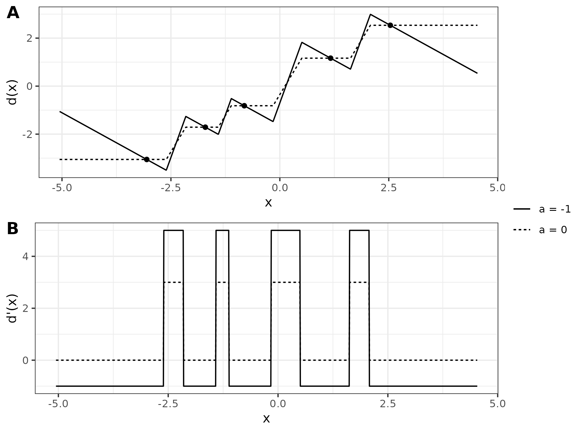
Figure 1: Two examples of absolutely continuous functions that satisfy $d_{\text{sawtooth},a}(X_{i})=X_{i}$ and $d_{\text{sawtooth},a}^{\prime}(X_{i})=a$ for every $i=1,\ldots,n$ and some $a\in\mathbb{R}$. Panel A plots $d_{\text{sawtooth},a}(x)$ functions and panel B shows their derivatives. The lines are labeled with their slopes, $a$, at each $X_{i}$. The dashed line is monotone non-decreasing.

Figure 1B suggests a way to resolve this problem. It shows that the derivatives $d_{\text{sawtooth},a}^{\prime}(x)$ are highly nonsmooth. Since it is the derivative that determines the penalty in $\hat{R}_{1}(d)$, this suggests that controlling the smoothness of $d^{\prime}(x)$ can control overfitting. A natural choice is a total variation-based shape constraint on $d^{\prime}(x)$. Indeed, Proposition 1 shows that as long as the total variation of $d^{\prime}(x)$ is not too large, functions like $d_{\text{sawtooth},a}(x)$ cannot exist.

Proposition 1.

Let $x_{1}<\dots<x_{n}$ and $d:\mathbb{R}\to\mathbb{R}$ be an absolutely continuous function. If $TV(d^{\prime})<2(n-1)$, then there exists an $i\in\{1,\dots,n\}$ such that either $d(x_{i})\neq x_{i}$ or $d^{\prime}(x_{i})\geq 0$.

Conveniently, the oracle minimizer $d^{*}(x)$ (2) has a derivative with manageable total variation. Proposition 2 characterizes this quantity, along with other properties of $d^{*}(x)$ that we will use to design a function class over which we will minimize $\hat{R}_{1}(d)$. In particular, Proposition 2 implies that $d^{*}(x)$ is always bound, absolutely continuous, and monotone non-decreasing.

Proposition 2.

The optimal separable estimator (2), $d^{*}(x)$, is bounded, monotone non-decreasing, and Lipschitz continuous; its derivative has bound total variation and is also Lipschitz continuous. Let $r(\theta)=\max_{i=1}^{n}\theta_{i}-\min_{i=1}^{n}\theta_{i}$ denote the range of $\theta_{1},\dots,\theta_{n}$. These bounds are summarized as:

1. $\min_{i=1}^{n}\theta_{i}\leq d^{*}(x)\leq\max_{i=1}^{n}\theta_{i}$

2. $0\leq d^{*\prime}(x)\leq\sigma^{-2}r(\theta)^{2}$

3. $TV(d^{*\prime})\leq\sigma^{-2}r(\theta)^{2}$

4. $\left\lvert d^{*\prime\prime}(x)\right\rvert\leq\sigma^{-4}r(\theta)^{3}$ .

Using Propositions 1 and 2, we can now choose a suitable function class for estimating $d^{*}(x)$. Observe that if $TV(d^{*\prime})<2(n-1)$, then we can find an upper bound on $TV(d^{\prime})$ that simultaneously prevents over-fitting of $\hat{R}_{1}(d)$ and ensures that $d^{*}(x)$ is in our function class. Since neither $TV(d^{*\prime})$ nor $r(\theta)=\max_{i=1}^{n}\theta_{i}-\min_{i=1}^{n}\theta_{i}$ are known when defining our function class, we specify data-dependent estimates for these quantities so that both of our desired properties hold simultaneously with high probability. We find a high probability upper bound on the range of $\theta_{1},\dots,\theta_{n}$ by expanding the range of $X_{1},\dots,X_{n}$ by a non-random quantity, $b_{n}>0$. We propose the following data-dependent function class:

$$\mathcal{D}_{1,n}=\left\{d:\mathbb{R}\to[\min_{i}X_{i}-b_{n},\max_{i}X_{i}+b_{n}]\mid d~{}\text{monotone non-decreasing},TV(d^{\prime})\leq\tau_{n}\right\},$$ (8)

where $b_{n}$ and $\tau_{n}=\sigma^{-2}(\max_{i=1}^{n}X_{i}-\min_{i=1}^{n}X_{i}+2b_{n})^{2}$ are constants that can depend on $X_{i}$, $\sigma$, and $n$. The inclusion of the monotonicity constraint is advantageous because from Proposition 2, $d^{*}(x)$ is always monotone non-decreasing. Note that the constraint $TV(d^{\prime})\leq\tau_{n}<\infty$ ensures that all of the functions in $\mathcal{D}_{1,n}$ are absolutely continuous.

We now need to ensure that $\mathcal{D}_{1,n}$ contains the oracle estimator $d^{*}(x)$. Lemma 1 implies that this will be true with high probability if $b_{n}$ is of the order $\{\sigma^{2}\log(n)\}^{1/2}$.

Lemma 1.

Let $b_{n}\geq 0$ be a non-random value that may depend on $\sigma$ and $n$, $\mathcal{D}_{1,n}$ be defined as in (8), and $d^{*}(x)$ be the optimal separable estimator (2). Then

$$P\left(d^{*}\not\in\mathcal{D}_{1,n}\right)\leq 6n\exp\left(\frac{-b_{n}^{2}}{2\sigma^{2}}\right).$$

In particular, when $b_{n}=(K\sigma^{2}\log n)^{1/2}$ for some $K\in\mathbb{R}$, the bound becomes $6n^{1-\frac{K}{2}}$, which can be made to converges to zero at an arbitrarily quick polynomial rate by selecting the correct $K>2$. We therefore define the following estimate of $d^{*}(x)$ using the function class using our data-dependent function class $\mathcal{D}_{1,n}$:

$$\hat{d}=\arg\min_{d\in\mathcal{D}_{1,n}}\hat{R}_{1}(d).$$ (9)

Theorem 1 shows that $\hat{d}(x)$ can be characterized as a piecewise linear function. The proof of Theorem 1 uses Carathéodory’s theorem for convex hulls (Carathéodory, 1911) to reduce the infinite dimensional optimization problem over $\mathcal{D}_{1,n}$ to a finite dimensional one, similar to the proof of Theorem 1 in Boyd et al. (2018). Notice that the range of $\hat{d}(x)$ always lies within $\left[\min_{i=1}^{n}X_{i},\max_{i=1}^{n}X_{i}\right]$, so in practice the role of $b_{n}$ is only needed for defining the high probability bound $TV(d^{*\prime})\leq\tau_{n}$.

Theorem 1.

For every $g\in\mathcal{D}_{1,n}$ (8), there exists a continuous, piecewise linear function, $\tilde{g}\in\mathcal{D}_{1,n}$ with at most $n+3$ knots, such that $\tilde{g}(X_{i})=g(X_{i})$ for $i=1,\dots,n$, $\sum_{i=1}^{n}\tilde{g}^{\prime}(X_{i})=\sum_{i=1}^{n}g^{\prime}(X_{i})$, and $\tilde{g}^{\prime}(x)=0$ for $x<\min_{i=1}^{n}X_{i}$ and $x>\max_{i=1}^{n}X_{i}$.

Based on Theorem 1 we implement $\hat{d}(x)$ as a piecewise linear function: $\hat{d}(x)=\beta_{0}+\sum_{j=1}^{M}\beta_{j}(x-x_{j})_{+}$, where $(y)_{+}=\max\{y,0\}$ and $x_{1}<x_{2}<\dots<x_{M}$ are a finite collection of fixed knots. The minimization of $\hat{R}_{1}(d)$ over $\beta_{i}$ and $x_{j}$ is non-convex, so in practice we approximate $\hat{d}(x)$ by fixing a regular grid of knots and only optimizing over $\beta_{i}$. We note that for fixed knots $x_{1}<x_{2}<\dots<x_{M}$, minimizing $\hat{R}_{1}(d)$ over $\beta_{i}$ is a convex problem that can be readily solved by many off-the-shelf convex optimizers. Other potentially viable strategies for rapidly finding a good set of knots include placing knots at each of the observations or their quantiles and iterative approaches that slowly accumulate knots, similar to Boyd et al. (2018, 2017). The performance of various knot placement strategies are compare in Appendix A of the Supplementary Material.

Once the knots are fixed, we approximate $\hat{d}(x)$ as:

$$\hat{d}(x) \approx\arg\min_{\beta_{0},\beta_{1},\dots,\beta_{M}\in\mathbb{R}}\sum_{i=1}^{n}\left\{X_{i}-\beta_{0}-\sum_{j=1}^{M}\beta_{j}(X_{i}-x_{j})_{+}\right\}^{2}+2\sigma^{2}\sum_{i=1}^{n}\sum_{j=1}^{M}\beta_{j}1(X_{i}\geq x_{j})$$

$$\text{subject to:}\quad\sum_{j=1}^{M}\beta_{j}=0,\quad\sum_{j=1}^{k}\beta_{j}\geq 0~{}\text{for}~{}k=1,\dots,M-1,\quad\sum_{j=1}^{M}|\beta_{j}|\leq\tau_{n},$$

where the constraints correspond to our bounded, monotone non-decreasing, and total variation constraints, respectively. We note that there are two interesting interpretations of this parameterization. First, when we place the knots at each of the observations, this estimator is a constrained, irregularly-spaced, degree-one trend-filter (Tibshirani, 2014b); the function constraints can be easily translated into the trend-filter parameterization. Second, this parameterization resembles a degree-one locally adaptive regression spines (Mammen and van de Geer, 1997) and one-dimensional MARS (Friedman, 1991); however, our minimization problem includes constraints and a slightly different penalty. We stick to the more general model described above for flexibility and ease of implementation.

Theorem 2 below shows that the conservative, high probability upper bounds on $TV(d^{*\prime})$ and $r(\theta)$ that we pursued in (8) produce an asymptotically optimal estimator. In practice, the choice of $\tau_{n}$ in the statement of Theorem 2 is usually too large and a smaller value may be more efficient; we describe some alternatives in Section 5.

Theorem 2.

Let $X_{i}\sim N(\theta_{i},\sigma^{2})$ for $i=1,\dots,n$ be independent such that $\sigma^{2}>0$ is known and assume $\max_{i=1}^{n}|\theta_{i}|<C_{n}$. Further, let $b_{n}=(3\sigma^{2}\log n)^{1/2}$ and $\tau_{n}=\sigma^{-2}(\max_{i=1}^{n}X_{i}-\min_{i=1}^{n}X_{i}+2b_{n})^{2}$. Define $\hat{d}(x)$ as in (9) and let $d^{*}(x)$ be the optimal separable estimator (2), then

$$R(\hat{d};\theta)-R(d^{*};\theta)=\mathcal{O}\left\{n^{-1/2}\left(C_{n}+\log^{1/2}n\right)^{2}\right\}.$$

The excess risk bounded in Theorem 2 is sometimes referred to as the compound regret (Efron, 2019; Polyanskiy and Wu, 2021). Our result implies that our constrained and penalized regression estimator can achieve asymptotically zero regret whenever $C_{n}=o(n^{1/4})$. When $C_{n}=o\left(n^{\epsilon}\right)$ for every $\epsilon>0$, the regret of our estimator is essentially of order $n^{-1/2}$. This matches the best known rate for this simultaneous estimation problem over an $\ell_{\infty}$ ball, achieved by the nonparametric $g$-modeling estimator $\hat{d}_{JZ}$ of Jiang and Zhang (2009), whose asymptotic ratio optimality result (3) can be translated to a regret that also scales like $n^{-1/2}$ (Polyanskiy and Wu, 2021).

Our proof of Theorem 2 leverages standard techniques for studying M-estimators. This leads naturally to bounds on the regret. An alternative quantity of interest would be the ratio of the two risks, as in (3). Bounding the ratio is more meaningful in settings where the optimal separable estimator may perform very well, such as when $\theta$ is sparse and the oracle risk $R(d^{*};\theta)$ already tends quickly toward zero. Studying the ratio optimality of our $\hat{d}$ would be an interesting direction for future work, and simulations in Section 5 already show that our estimator is comparable to the nonparametric empirical Bayes methods when estimating sparse $\theta$.

In our proof we use symmetrization and metric entropy bounds based on the size of $\mathcal{D}_{1,n}$ and the function class of its derivatives. Our total variation bound, based on Proposition 1, provides the needed control over the function class of derivatives, while the bounded and monotone non-decreasing constraints are used to control the size of $\mathcal{D}_{1,n}$. We note that the monotonicity constraint is not necessary for the proof and other function classes such as bound total variation or Lipschitz over a finite domain, may be used instead. However, these alternative function classes may increase the size of the function class, introduce additional tuning parameters, or slow the rate of excess risk convergence.

4 Removing Constraints with Biased Risk Minimization

Our estimator $\hat{d}(x)$ (9) above has both a monotonicity as well as a total variation constraint, and the latter is crucial to avoid overfitting. In contrast, in standard isotonic least-squares regression, a monotonicity constraint alone already offers sufficient regularization (van de Geer, 2000). A natural question is whether monotonicity alone might be sufficient for developing an asymptotically optimal estimator in the simultaneous estimation problem.

Investigating this question reveals an interesting connection between the constraints on $d(x)$ and the estimate of the oracle loss $R(d;\theta)$ (4). A closer inspection of the decomposition of this loss in (5) gives

$$R(d;\theta) =\frac{1}{n}\sum_{i=1}^{n}E\{X_{i}-d(X_{i})\}^{2}+2\sigma^{2}\int_{-\infty}^{\infty}d^{\prime}(x)f_{\theta}(x)dx-\sigma^{2},$$ (10)

where $f_{\theta}(x)=n^{-1}\sum_{i=1}^{n}\phi_{\sigma}(x-\theta_{i})$. Previously, we replaced the integral above with an empirical expectation to give $\hat{R}_{1}(d)$ (6), and we found that monotone functions could still overfit. The core problem was that the empirical expectation penalty could not control the shape of $d(x)$ for $x\neq X_{i}$ because the values of $d^{\prime}(x)$ for these $x$ do not affect the risk estimate; recall Figure 1. In contrast, the integral in (10) controls the shape of $d(x)$ for all $x$ in the support of $f_{\theta}(x)$, because all values of $d^{\prime}(x)$ would affect the risk.

This suggests that a monotonicity constraint would be sufficient to achieve asymptotical optimality given only a monotonicity constraint if we could find a continuous estimate $f_{\theta}(x)$ so that $d^{\prime}(x)$ is penalized over the whole domain of the estimator. Drawing on the kernel density estimator literature (Tsybakov, 2009), we use

$$\hat{f}_{h}(x)=\frac{1}{n}\sum_{i=1}^{n}\phi_{h}(x-X_{i})$$ (11)

for some bandwidth $h>0$. In the Bayesian setting, $\hat{f}_{h}(x)$ is equivalent to a Gaussian kernel estimate of the density $X_{i}$ marginalizing over the random $\theta_{i}$; however, we stress that our approach does not depend on this interpretation.

We propose the following function class for fitting estimators:

$$\mathcal{D}_{0,n}=\left\{d:\mathbb{R}\to[\min_{i}X_{i}-b_{n},\max_{i}X_{i}+b_{n}]\mid d~{}\text{monotone non-decreasing}\right\},$$ (12)

where $b_{n}$ is a constant depending on $\sigma$ and $n$. As in Lemma 1, $b_{n}$ is used to ensure that $\mathcal{D}_{0,n}$ contains the optimal separable estimator with high probability. This result can be established by noting that $\mathcal{D}_{1,n}\subset\mathcal{D}_{0,n}$ when the range of $\mathcal{D}_{0,n}$ is at least as large as range of $\mathcal{D}_{1,n}$. We would like to use plug our $\hat{f}_{h}(x)$ (11) into the loss decomposition (10) and minimize the result over functions in $\mathcal{D}_{0,n}$. Unfortunately, this is not well-justified because not all monotone functions are weakly differentiable, so Stein’s lemma cannot be directly applied. In order to justify a risk estimate for all functions in $\mathcal{D}_{0,n}$, Proposition 3 extends Stein’s lemma to apply to every bounded, monotone non-decreasing function. The proof of Proposition 3 draws heavily on a Corollary 1 in Tibshirani (2014a). Rather than extend Stein’s lemma to apply to all of $\mathcal{D}_{0,n}$, we could instead study a smoother function class that is a subset of $\mathcal{D}_{0,n}\cap\{d\mid d~{}\text{weakly differentiable}\}$; however, this may introduce additional tuning parameters or make it difficult to establish a parameterization for the optimal estimator.

Proposition 3.

Let $Z\sim N(\mu,\sigma^{2})$. Let $g:\mathbb{R}\to\mathbb{R}$ have finite total variation and let $\mathcal{J}(g)=\{t_{1},t_{2},\dots\}$ be the countable set of locations where $g$ has a discontinuity. Let $g^{\prime}$ be the derivative of $g$ almost everywhere and assume that $E|g^{\prime}(Z)|<\infty$. Then

$$\frac{1}{\sigma^{2}}E[(Z-\mu)g(Z-\mu)]=E[g^{\prime}(Z-\mu)]+\sum_{t_{k}\in\mathcal{J}(g)}\phi_{\sigma}(t_{k}-\mu)\left\{\lim_{x\downarrow t_{k}}g(x)-\lim_{x\uparrow t_{k}}g(x)\right\}.$$

Since every bounded, monotone non-decreasing function has finite total variation, we can combine Proposition 3 with (10) and (11) to find an estimate of the oracle loss $R(d;\theta)$ (4) that holds for every $d\in\mathcal{D}_{0,n}$:

$$\hat{R}_{0}(d;h)=\frac{1}{n}\sum_{i=1}^{n}\{X_{i} -d(X_{i})\}^{2}+2\sigma^{2}\int_{-\infty}^{\infty}d^{\prime}(x)\hat{f}_{h}(x)dt$$ (13)

$$+2\sigma^{2}\sum_{x_{k}\in\mathcal{J}(d)}\hat{f}_{h}(x_{k})\left\{\lim_{x\downarrow x_{k}}d(x)-\lim_{x\uparrow x_{k}}d(x)\right\}-\sigma^{2}.$$

This risk estimate is biased for fixed $h$, but minimizing it gives a useful estimate of $d^{\star}(x)$ when $h\downarrow 0$ at an appropriate rate with $n$. Because $\hat{f}_{h}(x)$ is positive for all of $\mathbb{R}$ and because only constant functions minimize both the penalty terms, $\hat{R}_{0}(d;h)$ almost surely cannot be over-fit by functions in $\mathcal{D}_{0,n}$.

We propose the following estimator using this new risk estimate:

$$\tilde{d}_{h}=\arg\min_{d\in\mathcal{D}_{0,n}}\hat{R}_{0}(d;h).$$ (14)

Theorem 3 below exactly characterizes $\tilde{d}_{h}(x)$ for any fixed value of $h>0$. This theorem is similar to Proposition 1 in Mammen and van de Geer (1997) except they study the standard total variation penalty and place knots at the data, while we study a weighted total variation penalty and place knots according to the weight function. In practice, the penalized least-squares regression formulation ensures that we can ignore $b_{n}$ because $\tilde{d}_{h}(x)$ always has a range within $[\min_{i=1}^{n}X_{i},\max_{i=1}^{n}X_{i}]$, so $\mathcal{D}_{0,n}$ is free of tuning parameters.

Theorem 3.

Let $h>0$. For every $g\in\mathcal{D}_{0,n}$ (12) that is right-continuous at $X_{1},\dots,X_{n}$, there exists a piecewise constant function, $\tilde{g}\in\mathcal{D}_{0,n}$, that has at most $n-1$ knots and satisfies $\tilde{g}(X_{i})=g(X_{i})$ from the right and $\hat{R}_{0}(\tilde{g};h)\leq\hat{R}_{0}(g;h)$. The knots of $\tilde{g}(x)$ lie at the minimum of $\hat{f}_{h}(x)$ between each consecutive order statistics of $X_{1},\dots,X_{n}$.

Theorem 3 provides both the existence and the finite parameterization of $\tilde{d}_{h}(x)$. This makes exactly finding $\tilde{d}_{h}(x)$ a convex optimization problem for any fixed $h>0$, unlike $\hat{d}(x)$ in the previous section. For a fixed $h>0$, finding the true knots can still be a somewhat time-intensive procedure and in practice placing the knots at the average of each consecutive pair of $X_{i}$ provides a good approximation and alleviates much of the computational burden. We further note that the true knots may not be worth finding because they minimize $\hat{R}_{0}(d;h)$, so they are random and may not be the best knots for minimizing the out-of-sample risk. Simulations comparing knot placement strategies are in Appendix A of the Supplementary Material. Once the knots are fixed, computing $\tilde{d}_{h}(x)$ can be performed using off-the-shelf convex optimization software.

We efficiently compute $\tilde{d}_{h}(x)$ using a tailored algorithm that builds on Theorem 3 and leverages the pool adjacent violators algorithm (Robertson et al., 1988; Best and Chakravarti, 1990). The goal is to transform (14) into an unpenalized isotonic regression problem. We assume that $X_{1}<\dots<X_{n}$ without loss of generality. We first note that $\tilde{d}_{h}(x)$ is a piecewise constant function, by Theorem 3, so the integral term in $\hat{R}_{0}(\tilde{d}_{h};h)$ (13) is zero and our penalty is linear. We adopt a degree-zero trend-filter parameterization (Tibshirani, 2014b) for $\tilde{d}_{h}(x)$, which letting $\tilde{d}_{h}(x)=\beta_{0}+\sum_{i=1}^{n-1}\beta_{i}1(x\geq x_{i})$ and setting $\beta_{0}=d(X_{1})$ and $\beta_{i}=d(X_{i+1})-d(X_{i})$. Now, for a fixed $h>0$ and knots $x_{1}<\dots<x_{n-1}$ from Theorem 3, we define

$$\mathbf{x} =\begin{bmatrix}X_{1}\\ \vdots\\ X_{n}\end{bmatrix}, \mathbf{d} =\begin{bmatrix}d(X_{1})\\ \vdots\\ d(X_{n})\end{bmatrix}, \mathbf{f}_{h} =\begin{bmatrix}\hat{f}_{h}(x_{1})\\ \vdots\\ \hat{f}_{h}(x_{n-1})\end{bmatrix}, \mathbf{D} =\begin{bmatrix}1&-1&0&\dots&0&0\\ 0&1&-1&\dots&0&0\\ \vdots&\vdots&\vdots&\ddots&\vdots&\vdots\\ 0&0&0&\dots&1&-1\end{bmatrix},$$

and express (14) as

$$\mathbf{\tilde{d}_{h}}=\arg\min_{d\in\mathcal{D}_{0,n}}\|\mathbf{x}-\mathbf{d}\|_{2}^{2}+2n\sigma^{2}\mathbf{w}_{h}^{\prime}\mathbf{d}-n\sigma^{2}=\arg\min_{d\in\mathcal{D}_{0,n}}\left\|\left(\mathbf{x}-n\sigma^{2}\mathbf{w}_{h}\right)-\mathbf{d}\right\|_{2}^{2},$$ (15)

where $\mathbf{w}_{h}=\mathbf{D}^{\prime}\mathbf{f}_{h}$ and the last equality absorbs the linear penalty into the least-squares loss, motivated by the work of Wu et al. (2015) on penalized isotonic regression. Since our minimization is now a monotone least-squares regression problem, the pooled adjacent violators algorithm can be used to efficiently compute $\tilde{d}_{h}(X_{i})$ for each $i=1,\dots,n$. Interestingly, (15) can be interpreted as an unpenalized isotonic regression of sorted and suitably modified $X_{i}$.

Theorem 4 shows that when $h>0$ is properly chosen, our $\tilde{d}_{h}(x)$ has asymptotically optimal regret. This result identifies a rate for $h\to 0$ that optimally trades-off the bias and variance of the risk estimate. In simulations, this asymptotic rate seems works well as a default value for $h$, and other standard kernel density bandwidth selection methods, such as Silverman’s rule-of-thumb and cross-validation of the mean integral squared error (Silverman, 1986; Tsybakov, 2009) can be used as well.

Theorem 4.

Let $X_{i}\sim N(\theta_{i},\sigma^{2})$ be independent such that $\sigma^{2}$ is known and $\max_{i}|\theta_{i}|<C_{n}$. Further, let $b_{n}=\{(8/3)\sigma^{2}\log(n)\}^{1/2}$ and $h_{n}>0$ such that $h_{n}\asymp\sigma n^{-1/6}$. Define $\tilde{d}_{h_{n}}(x)$ as in (14) and let $d^{*}(x)$ be the optimal separable estimator (2), then

$$R(\tilde{d}_{h_{n}};\theta)-R(d^{*};\theta)=\mathcal{O}\left\{n^{-1/3}\left(C_{n}+\log^{1/2}n\right)^{2}\right\}.$$

This result demonstrates that monotonicity alone can produce an asymptotically optimal estimator; however, the use of a larger function class results in a slower convergence of excess risk, likely due to the bias in the risk estimate (13). On the other hand, $\tilde{d}_{h}(x)$ can be approximately computed in $\mathcal{O}(n\log n)$ time by placing knots at the average of consecutive order statistics and using the fast Fourier transformation to approximate $\hat{f}_{h}(x)$. This suggests that $\tilde{d}_{h}(x)$ can be useful for large simultaneous estimation problems.

It is also possible to achieve asymptotic regret after removing the monotonicity shape constraint. Corollary 1 below demonstrates that the class of bounded functions with bounded total variation is sufficient. The tradeoff is that this introduces an additional tuning parameter, though this can be estimated using a conservative high probability upper bound as we did in Section 3. Removing the monotonicity constraint means that more general convex optimization software is required to fit the estimator; however, Theorem 3 still applies to this larger function class. The proof of Corollary 1 follows almost immediately from the proof of Theorem 4.

Corollary 1.

Let $X_{i}\sim N(\theta_{i},\sigma^{2})$ be independent such that $\sigma^{2}$ is known and $\max_{i=1}^{n}|\theta_{i}|<C_{n}$. Further, let $b_{n}=\{(8/3)\sigma^{2}\log(n)\}^{1/2}$, $\lambda_{n}=\max_{i=1}^{n}X_{i}-\min_{i=1}^{n}X_{i}+2b_{n}$, and $h_{n}>0$ such that $h_{n}\asymp\sigma n^{-1/6}$. Define the new function class:

$$\mathcal{C}_{0,n}=\left\{d:\mathbb{R}\to[\min_{i}X_{i}-b_{n},\max_{i}X_{i}+b_{n}]\mid TV(d)\leq\lambda_{n}\right\},$$

and the corresponding estimator $\bar{d}_{h_{n}}=\arg\min_{d\in\mathcal{C}_{0,n}}\hat{R}_{0}(d;h_{n})$. Let $d^{*}(x)$ be the optimal separable estimator (2), then

$$R(\bar{d}_{h_{n}};\theta)-R(d^{*};\theta)=\mathcal{O}\left\{n^{-1/3}\left(C_{n}+\log^{1/2}n\right)^{2}\right\}.$$

The estimators $\bar{d}(x)$ and $\tilde{d}_{h}(x)$ exhibit two interesting connections with empirical Bayes $f$-estimators. Firstly, as noted by Koenker and Mizera (2014), the monotonicity constraint is not necessary but it can improve the efficiency of nonparametric empirical Bayes estimators and removes a tuning parameter. Secondly, the monotone $f$-estimator proposed by Koenker and Mizera (2014) is a piecewise constant estimator, just like $\tilde{d}_{h}(x)$; however, because our $\hat{f}_{h}(x)$ is not necessarily a log-concave density, there is no guarantee that the two estimators are equal for any value of $h>0$.

5 Simulations

5.1 Methods

We compared the performances of our constrained SURE estimator (9), $\hat{d}(x)$, and monotone-only estimator (14), $\tilde{d}_{h}(x)$, to those of state-of-the-art nonparametric empirical Bayes estimators for the canonical Gaussian sequence problem. Specifically, we compared to the $g$-modeling $\hat{d}_{JZ}(x)$ of Jiang and Zhang (2009), using 300 regularly spaced knots along $[\min_{i=1}^{n}X_{i},\max_{i=1}^{n}X_{i}]$, and the $f$-modeling $\hat{d}_{BG}(x)$ of Brown and Greenshtein (2009), using their recommended bandwidth $h=\sigma(\log n)^{-1/2}$.

When fitting our $\tilde{d}_{h}(x)$, we made no attempt to tune the bandwidth and instead set it to its theoretically optimal rate from Theorem 4. Alternative bandwidth choices are explored in Appendix A of the Supplementary Material. When fitting our $\hat{d}(x)$, we pursued three distinct methods for selecting the total-variation constraint $TV(d^{\prime})\leq\tau_{n}$. The first method was to set $\tau_{n}$ equal to the high-probability upper bound $\sigma^{-2}\{\max_{i=1}^{n}X_{i}-\min_{i=1}^{n}X_{i}+(3\sigma^{2}\log n)^{1/2}\}^{2}$ studied in Theorem 2. The second method was to develop a plug-in estimate of $TV(d^{*\prime})$. We first estimated

$$d^{*\prime\prime}(x)=\sigma^{2}\frac{f_{\theta}^{(3)}(x)}{f_{\theta}(x)}-3\sigma^{2}\frac{f^{\prime\prime}(x)f^{\prime}(x)}{f_{\theta}(x)^{2}}+2\sigma^{2}\left\{\frac{f^{\prime}(x)}{f_{\theta}(x)}\right\}^{3}$$

by plugging-in $X_{i}$ for $\theta_{i}$ to estimate each of the $f^{(k)}_{\theta}(t)$ for each $k\in\{0,1,2,3\}$, then we used numerical integration to approximate $TV(d^{*\prime})=\int_{-\infty}^{\infty}|d^{*\prime\prime}(x)|dx$. In practice this often out-performed the conservative high-probability bound. The final method was to choose $\tau_{n}$ using $k$-fold cross-validation, where we estimated out-of-sample risk using $\hat{R}_{1}(d)$ (6) applied to the $\hat{d}(x)$ fitted on the training folds. In the results below we used $k=5$.

We fit $\tilde{d}_{h}(x)$ using knots at the average of each consecutive order statistic of $X_{1},\dots,X_{n}$, and we fit $\hat{d}(x)$ using 30 regularly spaced knots along $(\min_{i=1}^{n}X_{i},\max_{i=1}^{n}X_{i})$. Alternative knot placement strategies are explored in Appendix A. We provide R implementations of our methods in the cole package (https://github.com/sdzhao/cole). Figure 2 visualizes each of these estimators applied to the same data, along with the optimal estimator $d^{\star}(x)$ (2) as a reference.

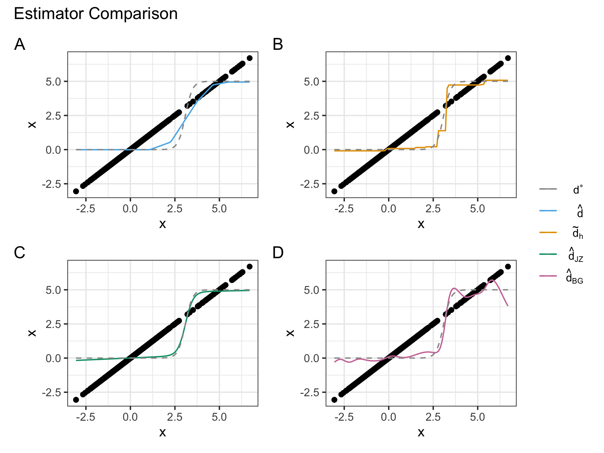
Figure 2: Visual comparison of different estimators on a sample of $n=1000$ data points. Solid points correspond to observed $X_{i}$. $d^{\star}$: oracle estimator (2); $\hat{d}$: proposed constrained SURE minimizer (9) using a plug-in estimate for $\tau_{n}$; $\tilde{d}_{h}$: proposed monotone-only estimator (14) using its theoretically optimal bandwidth; $\hat{d}_{JZ}$: estimator of Jiang and Zhang (2009); $\hat{d}_{BG}$: estimator of Brown and Greenshtein (2009).

5.2 High-Noise Setting

We first compared these methods under a standard high-noise setting where $X_{i}\sim N(\theta_{i},\sigma^{2})$ and $\sigma^{2}=1$. We fixed $n=1000$ and considered sparse configurations, where many of the $\theta_{i}$ were zero, and dense configurations, where all of the $\theta_{i}$ were nonzero. Estimation of sparse mean vectors has been thoroughly studied in the literature, for example by Johnstone and Silverman (2004), but there are many problems of interest, such as denoising gene expression levels from single-cell RNA-sequencing data (Huang et al., 2018; Li and Li, 2018), that are not well captured by the sparse model. Throughout, we evaluated the performance of each estimator using the sum of squared errors $\sum_{i=1}^{n}(\theta_{i}-\hat{\theta}_{i})^{2}$, where $\hat{\theta}_{i}$ is the corresponding estimate of $\theta_{i}$, averaged over 50 replications.

nonzero	5				50				500
$\mu$	3	4	5	7	3	4	5	7	3	4	5	7
$\hat{d}_{UB}$	84	66	58	38	214	154	88	50	528	357	176	57
$\hat{d}_{PI}$	41	39	33	24	169	128	69	29	500	345	166	38
$\hat{d}_{CV}$	47	43	36	21	171	123	65	31	479	311	145	41
$\tilde{d}_{h}$	42	37	31	17	179	126	65	25	485	316	150	33
$\hat{d}_{JZ}$	39	34	23	11	157	105	58	14	459	285	139	18
$\hat{d}_{BG}$	53	49	42	27	179	136	81	40	484	302	158	48

Table 1: Sums of squared errors for sparse normal mean vectors under high noise. $\hat{d}_{UB}$, $\hat{d}_{PI}$, and $\hat{d}_{CV}$: proposed constrained SURE estimator (9) with high-probability upper bound on $TV(d^{*\prime})$, plug-in estimate of $TV(d^{*\prime})$, and cross-validated $\tau_{n}$, respectively; $\tilde{d}_{h}$: proposed monotone-only estimator (14) using its theoretically optimal bandwidth; $\hat{d}_{JZ}$: estimator of Jiang and Zhang (2009); $\hat{d}_{BG}$: estimator of Brown and Greenshtein (2009).

In the sparse configuration, we followed Johnstone and Silverman (2004) and set $k\in\{5,50,500\}$ of the $\theta_{i}=\mu$ for $\mu\in\{3,4,5,7\}$, letting the remaining $\theta_{i}$ to zero. Table 1 reports the results, where the errors for the estimators of Jiang and Zhang (2009) and Brown and Greenshtein (2009) were copied from the corresponding papers. For $\hat{d}_{JZ}(x)$ we estimated the prior using convex optimization, as described by Koenker and Mizera (2014) and implemented in the REBayes R package of Koenker and Gu (2017). Our nonparametric regression estimators performed comparably to the nonparametric empirical Bayes estimators over a range of sparse settings. In most settings, $\hat{d}_{JZ}(x)$ had the best performance, followed closely by our $\tilde{d}_{h}(x)$, then our $\hat{d}(x)$, and finally by $\hat{d}_{BG}(x)$.

	Uniform(0, 5)	N(0,1)	Laplace(0,1)	0.5 N(-3,1) + 0.5 N(3,2)
$\hat{d}_{UB}$	709	566	546	853
$\hat{d}_{PI}$	647	514	501	794
$\hat{d}_{CV}$	653	520	507	800
$\tilde{d}_{h}$	670	532	523	834
$\hat{d}_{JZ}$	646	511	497	795
$\hat{d}_{BG}$	674	535	526	838

Table 2: Sums of squared errors for dense normal mean vectors under high noise. Estimators are the same as those in Table 1.

In the dense configuration, we generated $\theta_{i}$ by sampling them from an absolutely continuous prior distribution $G$ and then fixed them across replications. We considered a diverse collection of $G$: 1) the uniform distribution on $[0,5]$; 2) the Normal distribution with mean zero and variance of one; 3) the Laplace distribution with mean zero and variance of one; and 4) an asymmetric two-component Gaussian mixture with means at -3 and 3 and and variances of 1 and 2. These represent various tail bounds and problem complexities. In this scheme, the tail bound $E\max_{i=1}^{n}|\theta_{i}|$ plays the role similar to $C_{n}$ in our excess risk rate theorems. Table 2 reports the results and demonstrates a similar ranking of estimator performance as Table 1, though our $\hat{d}(x)$ with the plug-in estimate of $\tau_{n}$ works better than our $\tilde{d}_{h}(x)$ here. Our proposed estimators were more competitive with $\hat{d}_{JZ}(x)$ in dense configurations compared to the sparse configurations.

5.3 Low-Noise Setting

We also compared estimators under a low noise setting where we repeated the simulations in Tables 1 and 2 but set $\sigma^{2}=10^{-8}$. As mentioned in Section 1, this setting mimics more complex simultaneous estimation problems where observations have densities that can take extremely small values on most of the support of the unknown parameters. The introduction gave an example arising from multivariate linear regression. As another illustration, Saha and Guntuboyina (2020) and Soloff et al. (2021) studied nonparametric empirical Bayes estimation of $d$-dimensional $\theta_{i}$. In particular, if the observations $X_{i}\sim N(\theta_{i},I)$, where $I$ is the $d\times d$ identity matrix, they assume $\theta_{i}\sim G(t)$ and estimate $G(t)$ by maximizing

$$\prod_{i=1}^{n}\int\frac{1}{(2\pi)^{1/2}}\exp\left\{-\frac{1}{2}\sum_{j=1}^{d}(X_{ij}-t_{j})^{2}\right\}dG(t)$$

over discrete distributions supported on a pre-specified grid, where $X_{ij}$ is the $j$th coordinate of $X_{i}$. However, when $d$ is large, the density in the integrand can be extremely small at most of the grid points, which can cause difficulties for convex optimization software.

We encountered this exact difficulty in our low-noise univariate Gaussian sequence problem. The nonparametric empirical Bayes methods became less reliable. For example, in our simulations we tried to implement $\hat{d}_{JZ}(x)$ using convex optimization, but the underlying MOSEK optimizer frequently failed. We resorted to the EM approach of Jiang and Zhang (2009), and even there we needed to artificially left-censor low density values to equal the smallest positive floating-point number supported by our machine. In our results we report only the results of our EM-based implementation. Our plug-in estimate of $TV(d^{*\prime})$ suffered from numerical stability issues in this regime as well, so we do not report its performance.

nonzero	5				50				500
$\mu$	3	4	5	7	3	4	5	7	3	4	5	7
$\hat{d}_{UB}$	3.42	4.74	4.79	5.45	2.75	5.07	5.15	5.22	2.09	5.07	5.99	5.57
$\hat{d}_{CV}$	-17.76	-17.43	-17.58	-17.51	-17.41	-17.82	-17.79	-17.68	-17.69	-17.68	-17.85	-17.88
$\tilde{d}_{h}$	-17.78	-17.53	-17.70	-17.70	-17.95	-17.82	-17.78	-17.69	-17.70	-17.72	-17.84	-17.88
$\hat{d}_{BG}$	-11.52	-11.52	-11.52	-11.51	-11.50	-11.51	-11.50	-11.50	-11.51	-11.52	-11.51	-11.52
$\hat{d}_{JZ}$	-9.10	-9.21	-9.14	-9.12	-9.19	-9.17	-9.15	-9.15	-9.25	-9.29	-9.27	-9.28

Table 3: Natural logs of sums of squared errors for sparse normal mean vectors under low noise. The estimators used in this table are the same as those used in Table 1.

method	Uniform(0, 5)	N(0,1)	Laplace(0,1)	0.5 N(-3,1) + 0.5 N(3,2)
$\hat{d}_{UB}$	3.24	7.83	7.50	8.76
$\hat{d}_{CV}$	-1.40	-4.11	-2.42	-1.46
$\tilde{d}_{h}$	-10.93	-11.12	-11.16	-11.05
$\hat{d}_{BG}$	-11.52	-11.50	-11.51	-11.53
$\hat{d}_{JZ}$	6.97	6.38	6.44	9.19

Table 4: Natural logs of sums of squared errors for dense normal mean vectors under low noise. The estimators used in this table are the same as those used in Table 2.

Tables 3 and 4 report the performances of each estimator for sparse and dense configurations, respectively. Here we quantify performance using $\log\sum_{i=1}^{n}(\theta_{i}-\hat{\theta}_{i})^{2}$ averaged over 50 replications, where we take natural log because the sum of squared errors is otherwise already very low with such small noise. The results demonstrate that some of our proposed methods, with appropriate tuning, can match or outperform the state-of-the-art nonparametric empirical Bayes methods when $\sigma$ is small. Specifically, our monotone-only $\tilde{d}_{h}(x)$ (14) was the top performer in the sparse configurations and nearly matched the estimator of Brown and Greenshtein (2009) in the dense configurations. The $g$-modeling approach of Jiang and Zhang (2009), which was the top performer in the high-noise settings, had difficulty with such small $\sigma^{2}$.

6 Data analysis

We applied our proposed approaches to denoise spatial transcriptomic data. Spatial transcriptomics is a recently developed set of experimental techniques that can profile gene expression from regions of intact tissue sections at very high spatial resolution (Moffitt et al., 2022). This additional spatial information has the potential to revolutionize our understanding of biological processes and is one reason why these technologies were named “Method of the Year” in 2021 by the journal Nature Methods (Marx, 2021). Here we study data from a segment of the mouse small intestine, collected by Petukhov et al. (2022) using a spatial transcriptomic technique called MERFISH (Chen et al., 2015).

Despite its additional spatial context, these technologies still suffer from issues of detection efficiency and other experimental errors. The resulting measurements can thus be viewed as noisy observations of true expression levels. It has been demonstrated that denoising raw gene expression values can be a useful preprocessing step in non-spatial single-cell RNA-sequencing (Eraslan et al., 2019; Huang et al., 2018; Li and Li, 2018) and very recently in spatial transcriptomics (Wang et al., 2022).

In this section we apply our proposed simultaneous estimation methods to denoise MERFISH gene expression data from the mouse ileum. To formulate the problem, for a given cell let $Y_{i}$ denote the observed expression of gene $i$, for each of the $i=1,\ldots,241$ genes measured by Petukhov et al. (2022). We modeled the $Y_{i}$ as Poisson-distributed random variables and applied the Anscombe transform $X_{i}=2(Y_{i}+3/8)^{1/2}$ to obtain roughly normally-distributed $X_{i}$ with unit variance. Our goal was to denoise the $X_{i}$ by simultaneously estimating the $\theta_{i}=E(X_{i})$. Ideally we would measure the performance of estimates $\hat{\theta}_{i}$ using the mean squared error $\sum_{i}(\theta_{i}-\hat{\theta}_{i})^{2}/241$, but the true $\theta_{i}$ are unknown. We therefore approximated $\theta_{i}$ using the average expression of gene $i$ over the three cells closest to the cell being denoised. We denoised 1,000 randomly selected cells, shown in Figure 3.

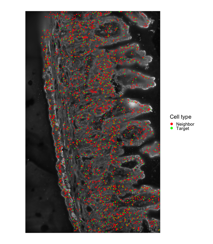
Figure 3: Spatial transcriptomic data from the mouse ileum (Petukhov et al., 2022). One thousand target cells (green) were randomly selected to be denoised, and the three nearest neighbors of each cell (red) were used to assess denoising accuracy.

We applied the following estimators: the observed $X_{i}$, our proposed regression-based estimators $\hat{d}_{CV}(x)$ (9) and $\tilde{d}_{h}(x)$ (14), and the state-of-the-art nonparametric empirical Bayes methods $\hat{d}_{BG}(x)$ (Brown and Greenshtein, 2009) and $\hat{d}_{JZ}(x)$ (Jiang and Zhang, 2009). The average mean squared errors across all 1,000 cells was 0.3845, 0.3599, 0.3794, 0.5881, and 0.4011, respectively. By this measure, our proposed methods were the best performers. For a more detailed comparison of the estimators, for each cell we subtracted the mean squared error of $\hat{d}_{JZ}(x)$ from the mean squared errors of the other estimators. Figure 4 plots the histograms of these differences and shows that our $\hat{d}_{CV}(x)$ and $\tilde{d}_{h}(x)$ outperformed $\hat{d}_{JZ}(x)$ on most of the cells.

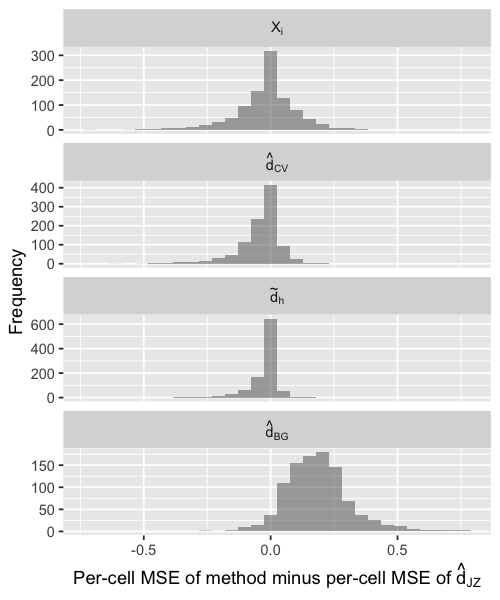
Figure 4: Histograms of the mean squared errors of different estimators minus the mean squared error of $\hat{d}_{JZ}(x)$ (Jiang and Zhang, 2009), for denoising the expressions of 241 genes in each of 1,000 randomly selected cells from the mouse ileum (Petukhov et al., 2022).

7 Discussion

Nonparametric empirical Bayes approaches to simultaneous estimation are the current standard, but are philosophically challenging to describe and also face performance issues when the measurement error noise is low. We have attempted to address these issues by showing that the problem can be formulated as penalized, self-supervised, nonparametric least-squares regression. This enabled us to apply empirical risk minimization ideas to construct estimators motivated entirely by frequentist ideas that can still achieve similar levels of accuracy, in theory and in simulations, as the state-of-the-art methods. Furthermore, our estimators can outperform existing methods in low-noise settings that model more complex simultaneous estimation problems.

One potential additional benefit of our regression perspective is that it can naturally accommodate complicated decision rules, for example those that leverage covariate or structural information to estimate each $\theta_{i}$. This information often arises in settings where there are replications (Ignatiadis et al., 2021), results from auxiliary experiments (Banerjee et al., 2020; Zhao, 2021), regular dependence structures (Greenshtein et al., 2019; Lehtinen et al., 2018), and known heteroskedastic variances (Weinstein et al., 2018; Xie et al., 2012, 2016; Tan, 2015; Zhao and Biscarri, 2021). Regression modeling offers a natural way to specific, either parametrically or nonparametrically, how the additional information is believed to be related to the $\theta_{i}$. A multi-dimensional version of Stein’s lemma can then be used derive corresponding risk estimates to be minimized. For example, given covariates $C_{i1},\ldots,C_{ip}$ in addition to each observation $X_{i}$, we could posit a generalized additive model $g(X_{i})+f(C_{i1},\dots,C_{ip})$ to estimate $\theta_{i}$ (Hastie and Tibshirani, 1986; Hastie et al., 2001). This decomposition is closely related to the hierarchical Bayesian model proposed by Ignatiadis and Wager (2019) under an empirical Bayes framework. For more complicated problems, modern deep learning architectures can be easily incorporated into our regression approach.

Finally, we conjecture that the performance of our estimators could be improved by incorporating additional shape constraints. For example, the nonparametric $g$-modeling estimator $\hat{d}_{JZ}(x)$ of Jiang and Zhang (2009) is, by construction, a Gaussian posterior mean, and therefore inherits a great deal of smoothness properties such as infinite, continuous, bounded derivatives. In contrast, this is not true of all functions in the two function classes we studied. It is possible that applying our framework to smaller classes of smoother functions would result in improved estimators. Related work by Zhao (2021), who applied empirical risk minimization over a function class motivated by the form of the oracle $d^{\star}(x)$ estimator, offers some evidence that this might be the case.

Supplementary Materials

The supplementary material contains additional simulations and the proofs of our main and supporting results.

References

- Akaike (1973) H. Akaike. Information theory and an extension of the maximum likelihood principle. 1973.
- Banerjee et al. (2020) T. Banerjee, G. Mukherjee, and W. Sun. Adaptive sparse estimation with side information. Journal of the American Statistical Association, 115(532):2053–2067, 2020. doi: 10.1080/01621459.2019.1679639. URL https://doi.org/10.1080/01621459.2019.1679639.
- Banerjee et al. (2021) T. Banerjee, Q. Liu, G. Mukherjee, and W. Sun. A general framework for empirical bayes estimation in discrete linear exponential family. Journal of Machine Learning Research, 22(67):1–46, 2021. URL http://jmlr.org/papers/v22/19-873.html.
- Best and Chakravarti (1990) M. J. Best and N. Chakravarti. Active set algorithms for isotonic regression; a unifying framework. Mathematical Programming, 47(1):425–439, 1990. doi: 10.1007/BF01580873. URL https://doi.org/10.1007/BF01580873.
- Boyd et al. (2017) N. Boyd, G. Schiebinger, and B. Recht. The alternating descent conditional gradient method for sparse inverse problems. SIAM Journal on Optimization, 27(2):616–639, 2017. doi: 10.1137/15M1035793. URL https://doi.org/10.1137/15M1035793.
- Boyd et al. (2018) N. Boyd, T. Hastie, S. Boyd, B. Recht, and M. I. Jordan. Saturating splines and feature selection. Journal of Machine Learning Research, 18(197):1–32, 2018. URL http://jmlr.org/papers/v18/17-178.html.
- Brown and Greenshtein (2009) L. D. Brown and E. Greenshtein. Nonparametric empirical Bayes and compound decision approaches to estimation of a high-dimensional vector of normal means. The Annals of Statistics, 37(4):1685 – 1704, 2009. doi: 10.1214/08-AOS630. URL https://doi.org/10.1214/08-AOS630.
- Carathéodory (1911) C. Carathéodory. Über den variabilitätsbereich der fourier’schen konstanten von positiven harmonischen funktionen. Rendiconti Del Circolo Matematico di Palermo (1884-1940), 32(1):193–217, 1911.
- Chen et al. (2015) K. H. Chen, A. N. Boettiger, J. R. Moffitt, S. Wang, and X. Zhuang. Spatially resolved, highly multiplexed rna profiling in single cells. Science, 348(6233):aaa6090, 2015.
- Efron (2004) B. Efron. The estimation of prediction error. Journal of the American Statistical Association, 99(467):619–632, 2004. doi: 10.1198/016214504000000692. URL https://doi.org/10.1198/016214504000000692.
- Efron (2011) B. Efron. Tweedie’s formula and selection bias. Journal of the American Statistical Association, 106(496):1602–1614, 2011. doi: 10.1198/jasa.2011.tm11181. URL https://doi.org/10.1198/jasa.2011.tm11181.
- Efron (2012) B. Efron. Large-scale inference: empirical Bayes methods for estimation, testing, and prediction, volume 1. Cambridge University Press, 2012.
- Efron (2014) B. Efron. Two Modeling Strategies for Empirical Bayes Estimation. Statistical Science, 29(2):285 – 301, 2014. doi: 10.1214/13-STS455. URL https://doi.org/10.1214/13-STS455.
- Efron (2019) B. Efron. Bayes, Oracle Bayes and Empirical Bayes. Statistical Science, 34(2):177 – 201, 2019. doi: 10.1214/18-STS674. URL https://doi.org/10.1214/18-STS674.
- Efron and Morris (1973) B. Efron and C. Morris. Stein’s estimation rule and its competitors–an empirical bayes approach. Journal of the American Statistical Association, 68(341):117–130, 1973. ISSN 01621459. URL http://www.jstor.org/stable/2284155.
- Eraslan et al. (2019) G. Eraslan, L. M. Simon, M. Mircea, N. S. Mueller, and F. J. Theis. Single-cell RNA-seq denoising using a deep count autoencoder. Nature Communications, 10(1):390, 2019.
- Fourdrinier et al. (2018) D. Fourdrinier, W. Strawderman, and M. Wells. Shrinkage Estimation. Springer Series in Statistics. Springer International Publishing, 2018. ISBN 9783030021856. URL https://link.springer.com/book/10.1007/978-3-030-02185-6.
- Friedman (1991) J. H. Friedman. Multivariate Adaptive Regression Splines. The Annals of Statistics, 19(1):1 – 67, 1991. doi: 10.1214/aos/1176347963. URL https://doi.org/10.1214/aos/1176347963.
- Greenshtein et al. (2019) E. Greenshtein, A. Mantzura, and Y. Ritov. Nonparametric empirical Bayes improvement of shrinkage estimators with applications to time series. Bernoulli, 25(4B):3459 – 3478, 2019. doi: 10.3150/18-BEJ1096. URL https://doi.org/10.3150/18-BEJ1096.
- Guo et al. (2020) F. R. Guo, J. McQueen, and T. S. Richardson. Empirical Bayes for large-scale randomized experiments: a spectral approach. arXiv preprint arXiv:2002.02564, 2020.
- Hastie and Tibshirani (1986) T. Hastie and R. Tibshirani. Generalized additive models. Statistical Science, 1(3):297–310, 1986. ISSN 08834237. URL http://www.jstor.org/stable/2245459.
- Hastie et al. (2001) T. J. Hastie, J. H. Friedman, and R. Tibshirani. The Elements of Statistical Learning: Data Mining, Inference, and Prediction. 2001.
- Huang et al. (2018) M. Huang, J. Wang, E. Torre, H. Dueck, S. Shaffer, R. Bonasio, J. I. Murray, A. Raj, M. Li, and N. R. Zhang. SAVER: gene expression recovery for single-cell RNA sequencing. Nature Methods, 15(7):539–542, 2018.
- Ignatiadis and Wager (2019) N. Ignatiadis and S. Wager. Covariate-powered empirical Bayes estimation. Advances in Neural Information Processing Systems, 32, 2019.
- Ignatiadis et al. (2021) N. Ignatiadis, S. Saha, D. L. Sun, and O. Muralidharan. Empirical bayes mean estimation with nonparametric errors via order statistic regression on replicated data. Journal of the American Statistical Association, 0(0):1–13, 2021. doi: 10.1080/01621459.2021.1967164. URL https://doi.org/10.1080/01621459.2021.1967164.
- James and Stein (1961) W. James and C. Stein. Estimation with quadratic loss. In Proceedings of the Fourth Berkeley Symposium on Mathematical Statistics and Probability, volume 1, pages 361–379, 1961.
- Jiang and Zhang (2009) W. Jiang and C.-H. Zhang. General maximum likelihood empirical bayes estimation of normal means. The Annals of Statistics, 37(4):1647–1684, 2009. ISSN 00905364, 21688966. URL http://www.jstor.org/stable/30243683.
- Johnstone (2019) I. M. Johnstone. Gaussian estimation: Sequence and wavelet models. Technical report, Department of Statistics at Stanford University, 2019. URL https://imjohnstone.su.domains/GE_09_16_19.pdf.
- Johnstone and Silverman (2004) I. M. Johnstone and B. W. Silverman. Needles and straw in haystacks: Empirical Bayes estimates of possibly sparse sequences. The Annals of Statistics, 32(4):1594 – 1649, 2004. doi: 10.1214/009053604000000030. URL https://doi.org/10.1214/009053604000000030.
- Kiefer and Wolfowitz (1956) J. Kiefer and J. Wolfowitz. Consistency of the maximum likelihood estimator in the presence of infinitely many incidental parameters. The Annals of Mathematical Statistics, pages 887–906, 1956.
- Kim et al. (2022) Y. Kim, W. Wang, P. Carbonetto, and M. Stephens. A flexible empirical Bayes approach to multiple linear regression and connections with penalized regression. arXiv preprint arXiv:2208.10910, 2022.
- Koenker and Gu (2017) R. Koenker and J. Gu. REBayes: an R package for empirical Bayes mixture methods. Journal of Statistical Software, 82:1–26, 2017.
- Koenker and Gu (2023) R. Koenker and J. Gu. Empirical bayes: Tools, rules, and duals. 2023.
- Koenker and Mizera (2014) R. Koenker and I. Mizera. Convex optimization, shape constraints, compound decisions, and empirical bayes rules. Journal of the American Statistical Association, 109(506):674–685, 2014. ISSN 01621459. URL http://www.jstor.org/stable/24247195.
- Lehtinen et al. (2018) J. Lehtinen, J. Munkberg, J. Hasselgren, S. Laine, T. Karras, M. Aittala, and T. Aila. Noise2Noise: Learning image restoration without clean data. In J. Dy and A. Krause, editors, Proceedings of the 35th International Conference on Machine Learning, volume 80 of Proceedings of Machine Learning Research, pages 2965–2974. PMLR, 10–15 Jul 2018. URL https://proceedings.mlr.press/v80/lehtinen18a.html.
- Li and Li (2018) W. V. Li and J. J. Li. An accurate and robust imputation method scImpute for single-cell RNA-seq data. Nature Communications, 9(1):997, 2018.
- Love et al. (2014) M. I. Love, W. Huber, and S. Anders. Moderated estimation of fold change and dispersion for RNA-seq data with DESeq2. Genome Biology, 15(12):1–21, 2014.
- Mallows (1973) C. L. Mallows. Some comments on cp. Technometrics, 15(4):661–675, 1973. ISSN 00401706. URL http://www.jstor.org/stable/1267380.
- Mammen and van de Geer (1997) E. Mammen and S. van de Geer. Locally adaptive regression splines. The Annals of Statistics, 25(1):387 – 413, 1997. doi: 10.1214/aos/1034276635. URL https://doi.org/10.1214/aos/1034276635.
- Marx (2021) V. Marx. Method of the Year: spatially resolved transcriptomics. Nature Methods, 18(1):9–14, 2021.
- Moffitt et al. (2022) J. R. Moffitt, E. Lundberg, and H. Heyn. The emerging landscape of spatial profiling technologies. Nature Reviews Genetics, 23(12):741–759, 2022.
- Muralidharan (2010) O. Muralidharan. An empirical Bayes mixture method for effect size and false discovery rate estimation. The Annals of Applied Statistics, pages 422–438, 2010.
- Petukhov et al. (2022) V. Petukhov, R. J. Xu, R. A. Soldatov, P. Cadinu, K. Khodosevich, J. R. Moffitt, and P. V. Kharchenko. Cell segmentation in imaging-based spatial transcriptomics. Nature Biotechnology, 40(3):345–354, 2022.
- Polyanskiy and Wu (2021) Y. Polyanskiy and Y. Wu. Sharp regret bounds for empirical bayes and compound decision problems, 2021. URL https://arxiv.org/abs/2109.03943.
- Rao and Molina (2015) J. N. Rao and I. Molina. Small area estimation. John Wiley & Sons, 2015.
- Robbins (1951) H. Robbins. Asymptotically subminimax solutions of compound statistical decision problems. In Proceedings of the second Berkeley symposium on mathematical statistics and probability, volume 2, pages 131–149. University of California Press, 1951.
- Robertson et al. (1988) T. Robertson, F. Wright, and R. Dykstra. Order Restricted Statistical Inference. Probability and Statistics Series. Wiley, 1988. ISBN 9780471917878.
- Robinson et al. (2010) M. D. Robinson, D. J. McCarthy, and G. K. Smyth. edgeR: a Bioconductor package for differential expression analysis of digital gene expression data. Bioinformatics, 26(1):139–140, 2010.
- Saha and Guntuboyina (2020) S. Saha and A. Guntuboyina. On the nonparametric maximum likelihood estimator for Gaussian location mixture densities with application to Gaussian denoising. The Annals of Statistics, 48(2):738 – 762, 2020. doi: 10.1214/19-AOS1817. URL https://doi.org/10.1214/19-AOS1817.
- Silverman (1986) B. W. Silverman. Density estimation for statistics and data analysis. 1986.
- Smyth (2004) G. K. Smyth. Linear models and empirical Bayes methods for assessing differential expression in microarray experiments. Statistical applications in genetics and molecular biology, 3(1), 2004.
- Soloff et al. (2021) J. A. Soloff, A. Guntuboyina, and B. Sen. Multivariate, heteroscedastic empirical Bayes via nonparametric maximum likelihood. arXiv preprint arXiv:2109.03466, 2021.
- Stein (1956) C. Stein. Inadmissibility of the usual estimator for the mean of a multivariate normal distribution. In Proceedings of the Third Berkeley symposium on mathematical statistics and probability, volume 1, pages 197–206, 1956.
- Stein (1981) C. M. Stein. Estimation of the mean of a multivariate normal distribution. The Annals of Statistics, 9(6):1135–1151, 1981. ISSN 00905364. URL http://www.jstor.org/stable/2240405.
- Stigler (1990) S. M. Stigler. The 1988 Neyman Memorial Lecture: A Galtonian Perspective on Shrinkage Estimators. Statistical Science, 5(1):147–155, 1990. ISSN 08834237. URL http://www.jstor.org/stable/2245901.
- Tan (2015) Z. Tan. Improved minimax estimation of a multivariate normal mean under heteroscedasticity. Bernoulli, 21(1):574–603, 2015. ISSN 13507265, 15739759. URL http://www.jstor.org/stable/43590231.
- Tibshirani (2014a) R. J. Tibshirani. Degrees of freedom and model search. Statistica Sinica, 2014a.
- Tibshirani (2014b) R. J. Tibshirani. Adaptive piecewise polynomial estimation via trend filtering. Annals of Statistics, 42:285–323, 2014b.
- Tsybakov (2009) A. B. Tsybakov. Introduction to Nonparametric Estimation. 2009.
- van de Geer (2000) S. A. van de Geer. Empirical Processes in M-Estimation. 2000.
- van der Vaart and Wellner (1996) A. van der Vaart and J. A. Wellner. Weak Convergence and Empirical Processes: With Applications to Statistics. Springer Series in Statistics. Springer, 1996. ISBN 9780387946405.
- Wainwright (2019) M. J. Wainwright. High-Dimensional Statistics: A Non-Asymptotic Viewpoint. Cambridge Series in Statistical and Probabilistic Mathematics. Cambridge University Press, 2019. doi: 10.1017/9781108627771.
- Wang et al. (2022) L. Wang, M. Maletic-Savatic, and Z. Liu. Region-specific denoising identifies spatial co-expression patterns and intra-tissue heterogeneity in spatially resolved transcriptomics data. Nature Communications, 13(1):6912, 2022.
- Wang and Zhao (2021) Y. Wang and S. D. Zhao. A nonparametric empirical Bayes approach to large-scale multivariate regression. Computational Statistics & Data Analysis, 156:107130, 2021.
- Weinstein et al. (2018) A. Weinstein, Z. Ma, L. D. Brown, and C.-H. Zhang. Group-linear empirical Bayes estimates for a heteroscedastic normal mean. Journal of the American Statistical Association, 113(522):698–710, 2018.
- Wu et al. (2015) J. Wu, M. C. Meyer, and J. D. Opsomer. Penalized isotonic regression. Journal of Statistical Planning and Inference, 161:12–24, 2015. ISSN 0378-3758. doi: https://doi.org/10.1016/j.jspi.2014.12.008. URL https://www.sciencedirect.com/science/article/pii/S0378375814002055.
- Xie et al. (2012) X. Xie, S. C. Kou, and L. D. Brown. Sure estimates for a heteroscedastic hierarchical model. Journal of the American Statistical Association, 107(500):1465–1479, 2012. doi: 10.1080/01621459.2012.728154. URL https://doi.org/10.1080/01621459.2012.728154. PMID: 25301976.
- Xie et al. (2016) X. Xie, S. C. Kou, and L. Brown. Optimal shrinkage estimation of mean parameters in family of distributions with quadratic variance. The Annals of Statistics, 44(2):564 – 597, 2016. doi: 10.1214/15-AOS1377. URL https://doi.org/10.1214/15-AOS1377.
- Xin and Zhao (2022) H. Xin and S. D. Zhao. A compound decision approach to covariance matrix estimation. Biometrics, 2022.
- Zhang (2003) C.-H. Zhang. Compound decision theory and empirical Bayes methods. Annals of Statistics, pages 379–390, 2003.
- Zhao (2021) S. D. Zhao. Simultaneous estimation of normal means with side information. Statistica Sinica, 2021.
- Zhao and Biscarri (2021) S. D. Zhao and W. Biscarri. A regression modeling approach to structured shrinkage estimation. Journal of the American Statistical Association, 0(0):1–11, 2021. doi: 10.1080/01621459.2021.1875838. URL https://doi.org/10.1080/01621459.2021.1875838.