Continual Learning with Foundation Models: An Empirical Study of Latent Replay

Abstract

Rapid development of large-scale pre-training has resulted in foundation models that can act as effective feature extractors on a variety of downstream tasks and domains. Motivated by this, we study the efficacy of pre-trained vision models as a foundation for downstream continual learning (CL) scenarios. Our goal is twofold. First, we want to understand the compute-accuracy trade-off between CL in the raw-data space and in the latent space of pre-trained encoders. Second, we investigate how the characteristics of the encoder, the pre-training algorithm and data, as well as of the resulting latent space affect CL performance. For this, we compare the efficacy of various pre-trained models in large-scale benchmarking scenarios with a vanilla replay setting applied in the latent and in the raw-data space. Notably, this study shows how transfer, forgetting, task similarity and learning are dependent on the input data characteristics and not necessarily on the CL algorithms. First, we show that under some circumstances reasonable CL performance can readily be achieved with a non-parametric classifier at negligible compute. We then show how models pre-trained on broader data result in better performance for various replay sizes. We explain this with representational similarity and transfer properties of these representations. Finally, we show the effectiveness of self-supervised (SSL) pre-training for downstream domains that are out-of-distribution as compared to the pre-training domain. We point out and validate several research directions that can further increase the efficacy of latent CL including representation ensembling. The diverse set of datasets used in this study can serve as a compute-efficient playground for further CL research. Codebase is available under https://github.com/oleksost/latent_CL.

1 Introduction

The goal of continual learning (CL) is to design machine learning (ML) algorithms that can learn tasks presented in the form of a non-stationary stream. The relevance of CL for practical ML applications is usually justified with a reduced computational cost as compared to offline retraining on all data seen so far. While in a hypothetical infinite compute regime CL can be trivially solved through offline retraining, in practice buffers of small numbers of samples per task are used – a strategy known as experience replay (ER). This strategy is known to be very versatile and applicable in large set of scenarios (Kalifou et al., 2019; Diethe et al., 2018; Lesort et al., 2019; Prabhu et al., 2020; Traoré et al., 2019; Belouadah and Popescu, 2018; Wu et al., 2019; Hou et al., 2019; Lesort, 2020; Douillard et al., 2020a) in comparison with other families of CL methods (Lopez-Paz and Ranzato, 2017; Mendez and EATON, 2021). In this work we largely focus on the setting of class incremental learning and ER as the strategy of choice.

Recent years have witnessed development of large scale models pre-trained on broad data – the so called foundation models. These models are intended to be universal feature extractors that can produce useful features for a large number of downstream tasks  (Bommasani et al., 2021). With the increasing popularity of such models as a foundation for downstream tasks, several recent works have explored their continual fine-tuning (Mehta et al., 2022; Wu et al., 2022; Ramasesh et al., 2022). At the same time, an emerging trend in computer vision (CV) and natural language processing (NLP) shows that such models can be used even without expensive fine-tuning of the feature encoder (Devlin et al., 2018; Brown et al., 2020) or in zero-shot manner (Sanh et al., 2021; Radford et al., 2021; Zhai et al., 2022).

In this work, motivated by this trend, we explore how frozen foundation models can be effective for CL. This strategy is justified by its increased compute efficiency, potential to mitigate data privacy concerns (Desai et al., 2021), better sample efficiency, as well as potential reduction of CL to training a non-parametric models that do not forget by design.

For this, we conduct an extensive analysis of CL using the ER strategy applied in the latent space of pretrained models (latent ER) using 26 different large-scale models pre-trained on a variety of datasets, architectures and with different pre-training algorithms. We use 5 different raw data streams with varying degree of relatedness to the pre-training domain. Encoding these streams with the pre-trained encoders resulted in a set of 130 encoded CL streams, each being effectively a distinct task sequence with distinct intrinsic properties such as task complexity, similarity, relatedness, etc.. This allows us to study CL as a function of data and not, as traditionally done, as a function of CL algorithm.

Our main contributions can be summarized as following. (1) We contrast latent ER with the traditional strategy of fine-tuning the whole model and replaying raw data (end2end ER). The comparison is done in terms of the compute-accuracy trade-off and we find that, while being almost two orders of magnitude more computationally expensive, end2end ER leads to substantial accuracy improvement only on streams that are outside of the pre-training domain (OOD streams). At the same time, on all tested streams we have found an encoder that lead to final CL accuracy better or comparable to the best fine-tuned model. (2) We present a data driven empirical investigation of latent CL with various datasets and describe how characteristics, such as transfer and interference, usually associated to CL algorithms’ performance, can be heavily dependent on the properties of the data. (3) The analysis and the conclusions that we draw from the experiments help us to better understand the link between the characteristics of the encoded data distribution, properties of the pre-training procedure and the behaviour of downstream CL algorithms trained on it. We further detail the importance of these contributions in Appendix  A.

2 Related Works

Pretrained models. Transfer learning is one of the most successful paradigms in deep learning (Yosinski et al., 2014). Most computer vision systems start from ImageNet pre-trained weights (Ren et al., 2015; Chen et al., 2017; Carion et al., 2020). A recent papers on natural language processing (NLP) indicate that SSL of large transformer models (Devlin et al., 2018; Reddy et al., 2021; Douillard et al., 2021) on vast amounts of pre-training data results in models that, without further training, generalize well to new tasks from few examples (Brown et al., 2020) and perform well in zero-shot learning tasks (Sanh et al., 2021). In the field of computer vision, CNN and transformer-based models are starting to match the performance of supervised models on ImageNet (Caron et al., 2021; Tomasev et al., 2022). In this work, we investigate whether such pre-trained representations can be leveraged to achieve CL from frozen features.

Pre-training in CL can be either considered (a) as a post-deployment learning of the first task of the CL stream (internal pre-training) or (b) as a prior to deployment training on another dataset for which forgetting is not considered (external pre-training). In (a),  Castro et al. (2018) discarded the first task performance considered as “pre-training.”  Gallardo et al. (2021) remarked that the larger (w.r.t. number of classes) the initial task was, the more class-agnostic the feature extractor became, further exacerbated with SSL pre-training, and consequently leading to less forgetting. In (b), pre-training in the classical sense on a large external dataset (e.g. ImageNet (Deng et al., 2009)), except specific applications (e.g. segmentation (Cermelli et al., 2020), meta CL (Caccia and Pineau, 2021; Caccia et al., 2020; Javed and White, 2019)), is rarely used in CL. Hayes et al. (2018); Lesort et al. (2021b); Chrysakis and Moens (2020); Banayeeanzade et al. (2021) used a ResNet pretrained on ImageNet and then transferred a sequence of tasks. The two formers kept the pretrained feature extractor frozen during the continual training. More recently, Mehta et al. (2022) remarked that pre-training, for both NLP and CV, done on a diverse dataset significantly reduced forgetting in downstream CL tasks. Wu et al. (2022) investigated large NLP models (both encoders-decoders and decoders based) and concluded on the existence of robust early layers thanks to the SSL pre-training but remarked that middle and late layers still heavily suffered from forgetting. Finally, echoing Gallardo et al. (2021), Hu et al. (2022) showed that SSL was also important for external pre-training.

Latent replay methods propose to store or generate activations from intermediate layer(s) of a neural network, which are then replayed at the same intermediate layers to prevent forgetting when new tasks are learned during the CL process. While originally motivated through the lance of biological plausibility, this approach have shown some success. This method has also a lot of potential for various applications that we detail in appendix section A. Intuitively, latent replay methods assume that low level representations can be better shared across tasks and hence require less adaptation. To this end low layers are either regularized (Liu et al., 2020), trained at a slower pace (Pellegrini et al., 2020), or, as. in (van de Ven et al., 2020; Hayes et al., 2020), frozen. Freezing the low layers significantly reduces the computational cost of CL through reducing the amount of trainable parameters. These methods rely on the assumption that feature extractor can produce meaningful features and should be preferred in applications with limited compute.

Other existing CL approaches can be roughly clustered into regularization based (Kirkpatrick et al., 2017; Aljundi et al., 2017), dynamic architectures based methods (Yoon et al., 2017; Schwarz et al., 2018), which include modular methods (Mendez and EATON, 2021; Veniat et al., 2021; Ostapenko et al., 2021), and constrained optimization based methods (Lopez-Paz and Ranzato, 2017; Chaudhry et al., 2018).

3 Methodology

We first introduce the different pre-training models and datasets and discuss the latent replay strategy. We then introduce the class and task similarity measures used as well as a distinction we make between in- and out-of-distribution streams.

3.1 Setting and problem statement

Encoders. We consider a total of up to 32 encoders (most experiments used 26) with either ResNet (He et al., 2020) or Vision Transformer (ViT) (Dosovitskiy et al., 2020) architectures. These are pre-trained using different objectives, and amount of data, in order to assess how these properties affect CL performance. See model details in App. E.2.

Classifiers. We use a simple multi-layer perceptron (MLP) and non-parametric models as classifiers. The MLP classifier is endowed with 1 hidden layer of 1024 units. The 2 non-parametric metric-based classifiers are the nearest mean classifier (NMC) and streaming linear discriminant Analysis (SLDA) (Shaoning Pang et al., 2005), both do not require replay. NMC makes predictions by selecting the class corresponding to the nearest class prototype, where prototypes are the means of all samples in the class. SLDA represents each learned class using running means by class and features covariance matrix. It makes predictions by pondering distance with running means and covariance values (details in App. C).

Datasets. We consider six different datasets for downstream tasks. CUB-200 (Welinder et al., 2010) which contains 6K images of birds distributed in 200 different categories. Cars196 (Krause et al., 2013), which is formed 16,185 images of 196 classes of cars. CIFAR-100 (Krizhevsky et al., 2009) contains 60K images distributed in 100 categories. DTD (Cimpoi et al., 2014), a texture dataset, consisting of 5640 images, organized in 47 categories. The Oxford Pet dataset (Parkhi et al., 2012), which is a 37 category pet image dataset with roughly 200 images per class. FGCVCAircraft (Maji et al., 2013), which contains 10,200 images of aircrafts, with 100 images for each of the 102 classes.

Dataset Encoding and Scenarios. For each dataset, we encode all its examples using each of the pre-trained models. We do this once, as a pre-processing step before applying CL algorithms. For ResNet-based models, we extract the embeddings of the last layer, after global average pooling. For transformer-based models we extract the [CLS] or [EOS] token, as it is common procedure (Dosovitskiy et al., 2020; Radford et al., 2021). For models that use batchnorm (Ioffe and Szegedy, 2015), we use the pre-trained statistics and we do not update them during feature extraction. Models from timm include their own data-preprocessing functions. For other models, such as dino (Caron et al., 2021), we resize images to 224$\times$224 and standardize them with ImageNet statistics (except for the CIFAR100 dataset, which is resized to 100x100).

The encoding pipeline is provided by continuum (Douillard and Lesort, 2021), including the formation of CL streams. We used those datasets to create class-incremental scenarios, i.e. a new task brings new classes (van de Ven and Tolias, 2019; Lesort et al., 2021a). For most experiments, we evaluate models on a single dataset, which results from splitting a dataset into five different class groups (tasks) and learning each task in a sequence. We also consider a CL multi-dataset stream, which introduces each of the six different datasets in a sequential manner, resulting in six different tasks.

Metrics and variables of interest. In Tab. 1, we report the various metrics and their description. We also explore some variables of interest to better understand downstream performance: pre-training data, models architecture, number of parameters, pre-training FLOPS, and latent dimension size.

3.2 Approach: Latent Replay

To fairly compare models with different replay buffer sizes we use a replay buffer sampling strategy that ensures that each class (new and replayed) is sampled with the same probability during learning, guaranteeing a learning setting close to iid at each task. This amounts to oversampling/under-sampling the replay buffer samples if the number of samples per-class in the new task is larger/smaller than the per-class replay buffer. Even if not very sample efficient, this strategy avoids imbalanced datasets problems and enables a normalized comparison. It is important to note that in this replay strategy the more past classes were learned, the higher the per-epoch computation cost of the current task will be.

Table 1: A summary of CL metrics of interest.

Name	Description	Comments
$A_{\scaleto{CL}{3pt}}^{\scaleto{MLP}{4pt}}$	CL Accuracy	Accuracy on all tasks seen so far. Unless stated otherwise, measured at the end of the stream.
$A_{\scaleto{CL-reinit}{4pt}}^{\scaleto{MLP}{4pt}}$	$A_{CL}^{MLP}$ with re-initialization	Accuracy on tasks seen so far when weights are reinitialized at the beginning of each new task.
$A_{\scaleto{CL}{3pt}}^{\scaleto{NMC}{4pt}}$	Nearest Mean Classifier Accuracy	This accuracy is computed by a nearest mean classifier with Euclidean distance.
$A_{\scaleto{CL}{3pt}}^{\scaleto{SLDA}{4pt}}$	Streaming LDA Accuracy	CL accuracy of the SLDA classifier (Shaoning Pang et al., 2005).
$A_{i,t}$	Single task accuracy (acc. task)	Accuracy of task $i$ measured at time $t$.
$A_{task-cl}$	Mean task accuracy (acc. task cl)	Average of single task accs.: $A_{task-cl}=\frac{1}{T}\sum_{i=0}^{T-1}A_{i,i}$. Measured for different ER buffer sizes.
$A_{task-FS}$	Mean task Accuracy Few-Shot (FSH)	Like $A_{task-cl}$, but trained with 2 data points per class, no ER buffer and re-initialization.
$A_{iid}$	IID Accuracy (upper bound)	Accuracy realized on a dataset in an IID setting (no CL).
$A_{task-iid}$	Mean task acc. IID (acc task iid)	Similar to $A_{task-cl}$, but without replay, i.e. avv. acc. when each task is learned separately.
Interference total	$A_{task-iid}-A_{iid}$	Estimates the adverse effect of learning tasks together versus one.
Interference	$A_{task-iid}-A_{task-cl}$	Estimates the adverse effect of learning tasks with a given ER buffer versus one by one.
Transfer	$A_{CL}^{MLP}-A_{cl-reinit}^{MLP}$	Estimates the amount of knowledge transferred through time/tasks in the weights.
$F_{CL}^{MLP}$	Forgetting / Relative Forgetting	Forgetting is $A_{task-cl}-A_{cl}^{mlp}$. Relative forgetting is $F_{R_{T-1}}=\frac{1}{T}\sum_{t=0}^{T-1}\frac{A_{task_{t:t}}-A_{task_{t:T-1}}}{A_{task_{t:t}}}$.

3.3 Task and Classes Similarity

Several recent works have investigated the role of task similarity for catastrophic forgetting (Nguyen et al., 2019; Ramasesh et al., 2021; Lee et al., 2021). In this work we use task similarity measured in the latent space of large pretrained models as a tool to better understand the CL performance of latent ER models. Moreover, it provides a supplementary justification to the ID / OOD distinction that we introduce in the next section. We use two different similarity measures. (1) We extend the idea of subspace overlap, recently introduced by Ramasesh et al. (2021) to longer task sequences (details in appendix D). Importantly, similarity measures can not be used for algorithmic decision making at CL time when they assume access to future tasks’ data (as is the case for subspace overlap). (2) We measure inter-class similarity, which can be computed prior to learning a new task, hence this is an actionable measurement that can be used by a CL algorithm. We detail how both similarity metrics are calculated in Appendix D.

3.4 In-Distribution (ID) vs Out-of-Distribution (OOD)

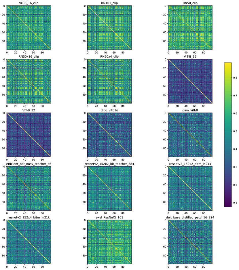
(a) Classes Similarity CIFAR100

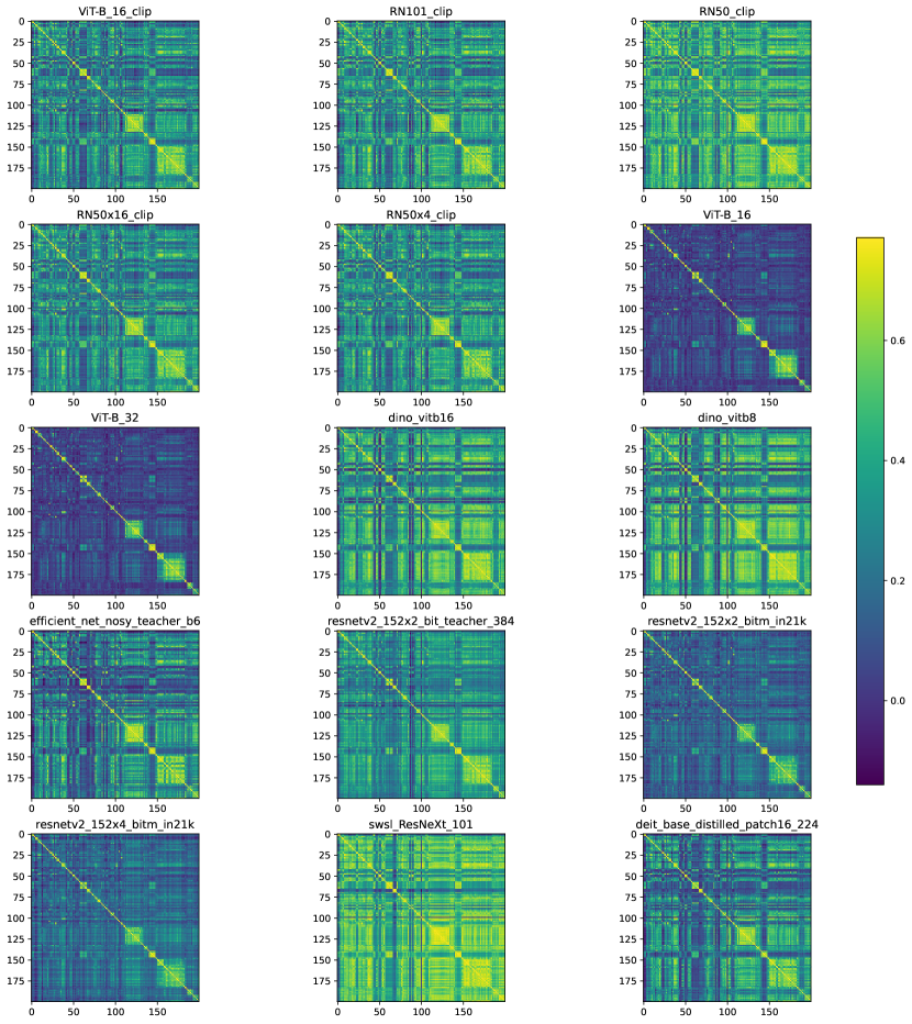
(b) Classes Similarity CUB200

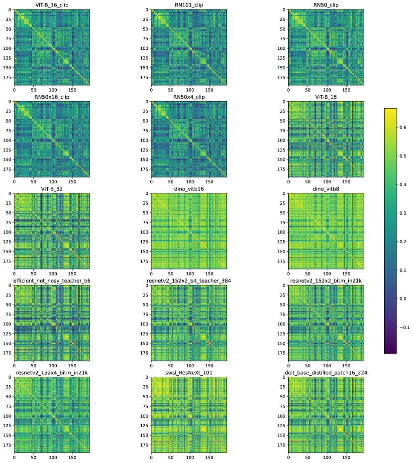
(c) Classes Similarity Cars196

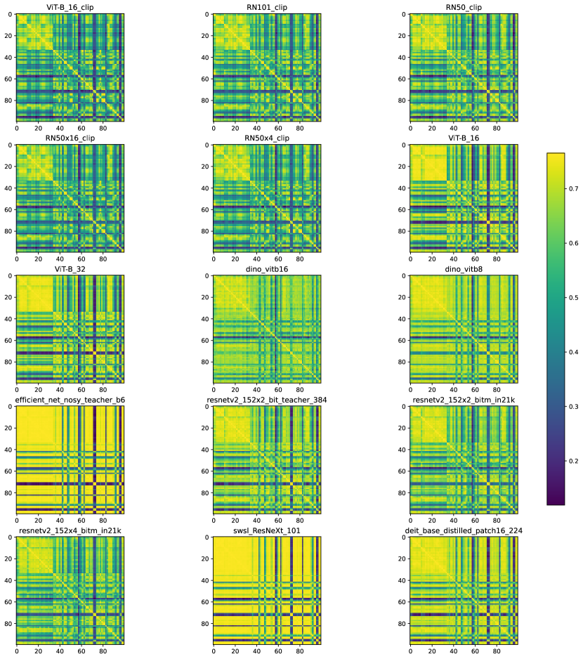
(d) Classes Similarity FGVCAircraft

Figure 14: Classes similarities with various encoders and datasets. Matrices represent cosine similarities between classes. The cosine similarity is computed by computing the mean of features (the prototype) for a given model and computing the cosine similarity between prototypes. By comparing all prototypes we get the matrices here. Blue color represents low cosine similarity, i.e. vectors are more orthogonal, yellow color represents high cosine similarity, i.e. vectors are less orthogonal. In our experiments, the brighter the matrices is the more OOD the dataset is from the pretraining data. NB: the more orthogonal the vector the easier the classification task is.

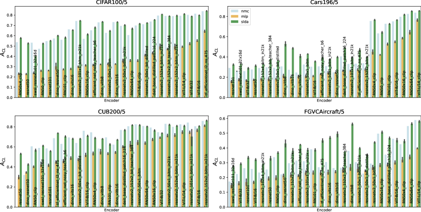
(a) ER buffer 2

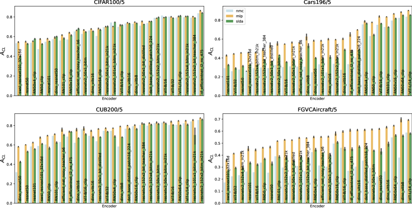
(b) ER buffer 50

Figure 25: MLP classifier vs. metric based classifiers performance on 4 streams.

We study the CL in two regimes. Each regime is characterized by the relationship between the source domain, i.e. pre-training data, and the target downstream tasks’ domain: (1) the in-distribution (ID) and (2) out-of-distribution (OOD) regimes. In our setting, the ID datasets are CIFAR100 and CUB200. ID dataset contain classes from the pre-training data (e.g. CIFAR100 and 52 classes of birds are in the ImageNet Wen et al. (2022)), while OOD dataset have different classes. The datasets that we consider OOD are FGCVAicraft and Cars196. These datasets contain samples of cars and airplanes, respectively. Notably, while the super-classes “car” and “airplane” are present in the pre-training datasets such as ImageNet1K and ImageNet21k, the level of supervision provided by these pre-training datasets (e.g. cars vs. everything else) is not sufficient to result in the ability to distinguish fine-grained classes of cars (e.g. “Acura TL Sedan 2012” vs. “Acura TSX Sedan 2012”) or airplanes (we confirm this in Section 4). Note, that we do not know exactly what data CLIP models are trained with. Hence, we do not include CLIP models in the ID versus OOD analysis. The exceptionally high performance of CLIP models on Cars196 dataset (see Fig. 25) and low inter-class similarity (see Fig. 14) indicate that classes from this dataset are likely to be part of the CLIP’s data.

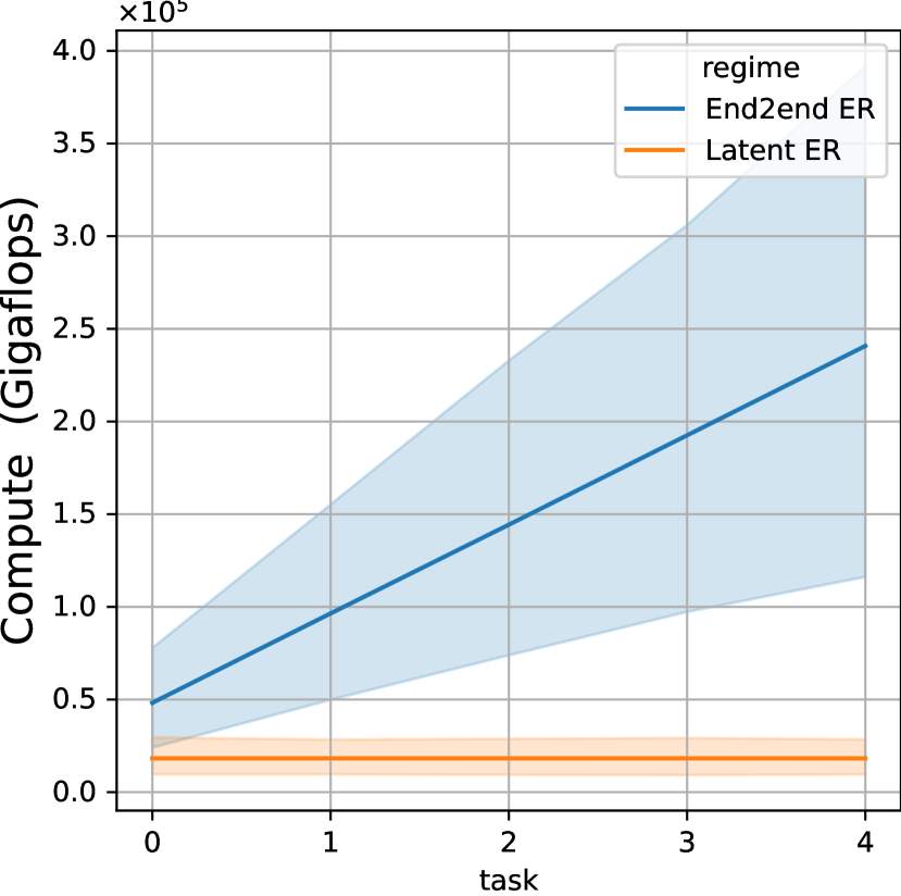
(a) Stream level growth

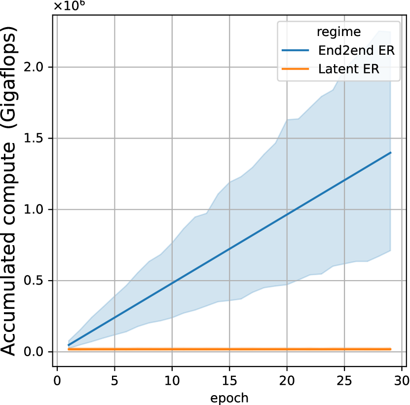
(b) Task level growth

Figure 1: Compute growth estimation (a) compute per epoch for each new task (not accumulated) throughout the tasks of CIFAR100/5 for latent ER (including the encoding compute) and end2end ER. (b) Compute growth within the first task of CIFAR100/5 for latent ER and end2end ER regimes (accumulated). In both plots we average over encoders and task orderings (5). In the compute estimation we approximate the cost of a backward pass as twice the cost of the forward pass. Latent ER compute growth (orange line) is dominated by end2end ER’s compute to an extend that it does not appear to grow at all.

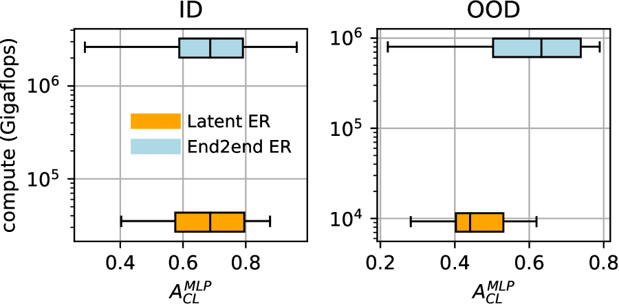
Figure 2: Compute-accuracy trade-off of end2end ER vs. latent ER strategies. We perform end2end fine-tuning with end2end ER for 7 different feature encoders on 4 streams with 3 different ER buffer sizes (10,30,50) and with a fixed task order. Here we compare resulting accuracy (x-axis) and average compute (per category, y-axis) on both ID (left) and OOD (right) streams. A detailed per model view is in Fig. 11. On average, end2end ER strategy results in a substantial performance improvement on OOD streams at the expense of almost 2 orders of magnitude more compute. As expected, no improvement is observed for ID streams.

An interesting insight from in-distribution (ID) and out-of-distribution (OOD) is in the Appendix, Fig. 14. We observe that ID classes have lower inter-class similarity than OOD classes. We hypothesize that this is due to the fact that OOD datasets are fine-grained and the pre-trained encoders are mapping all samples around the same class prototype.

4 Experimental Results

In this section we discuss our main findings. We first compare latent experience replay (ER) and end2end ER by reporting how they trade-off computational cost and accuracy. We then analyse latent ER strategies in terms of the relationship between pre-training and downstream-task data. We finalize with an encoder-level analysis.

4.1 Computational cost comparison: latent ER vs. End2end ER

Latent ER scales better in terms of compute.

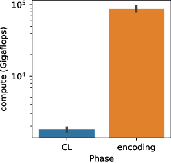
Figure 20: Average computational cost per phase. Encoding requires almost 2 orders of magnitude more compute.

The most obvious advantage of latent ER is the reduced compute and memory cost as compared to the conventional end2end ER. In Fig. 2 we compare the computational cost of latent ER with the end2end ER strategies. More specifically, we look at the growth pattern of the computational cost at a stream level (as new tasks are introduced) and at a task level (over epochs). In both cases computational cost of the end2end ER grows at a much larger rate making latent ER compute appear constant. Importantly, latent ER only needs to perform one forward path per sample through the (large) encoder in order to produce the latent representation of tasks, i.e. encode the data. This process constitutes a much larger portion of the overall computation cost than the subsequent CL phase on the encoded data (see Fig. 20 for comparison). Once encoded, the model can perform several epochs on the same encoded data. On the other hand, the end2end ER strategy has to complete a forward and a backward pass through the entire model for each sample. This leads to a much larger per epoch computational cost of end2end ER strategy as compared to latent ER, resulting in a steep increase of accumulated compute over the course of learning of a task as shown in Fig. 2b. As for the stream-level growth pattern shown in Fig. 2a, when encountered with a new task, the learner has to learn from the new examples and the examples from the replay buffer. This results in a increasing per epoch cost as new tasks are introduced. As discussed in Section 3.2, we use the oversampling and under-sampling strategies to avoid the class imbalance problems cause by new tasks having much mode samples per class than tasks in the replay buffer. It is important to mention that more elaborate replay strategies (Aljundi et al., 2019a; b; Bagus and Gepperth, 2021) can be used. These are likely to have equal effect on the scaling properties for both latent and end2end ER. While exploring such strategies is out of this study’s scope, we believe that the extent to which latent ER is more compute efficient than end2end ER should be similar for other ER strategies.

Compute-accuracy trade-off.

The computational advantage of latent ER can be only realized if the resulting accuracy is comparable to the accuracy of end2end ER. Here we investigate this compute-accuracy trade-off. For this we fine-tuned 7 encoders (both ViT and ResNet architectures, supervised and self-supervised pre-training, details in Appendix B) on 4 streams. As we show in App. Fig. 11, for each stream we find an encoder for latent ER that results in a better or comparable performance to the performance of the best end2end ER model tested. Thereby latent ER has a substantially smaller computational cost. In Figure 2 we give a consolidated view of the compute-accuracy trade-off for both ID and OOD streams. In the ID streams end2end ER even leads to a slight decrease in the CL performance on average as compared to latent ER. We observe that end2end ER results in a considerable performance improvement on the OOD streams on average, at the expense of almost two orders of magnitude more compute.

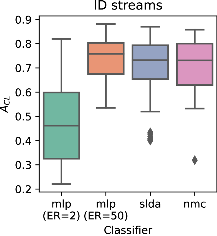
(a) ID streams

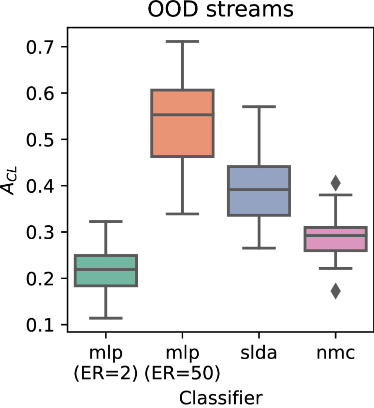
(b) OOD streams

Figure 3: ID vs. OOD comparison of the metric based classifiers NMC and SLDA, and replay based MLP in high and low ER buffer size regimes. For ID streams the CL accuracy of metric based classifiers is close to the accuracy of replay based MLP in the large ER buffer regime.

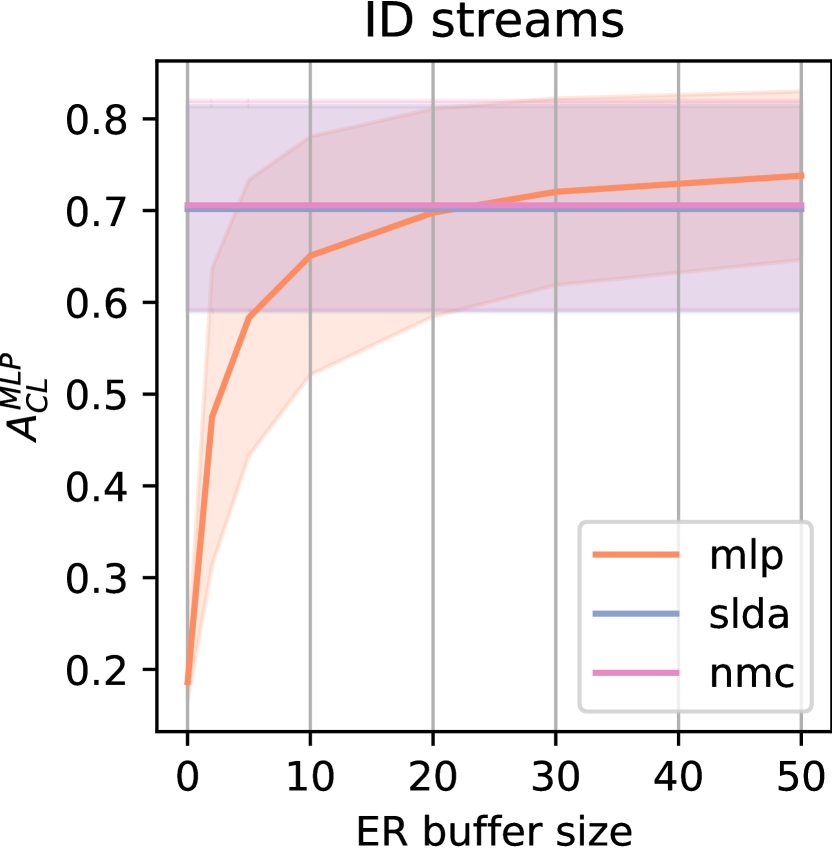
(c) ID streams

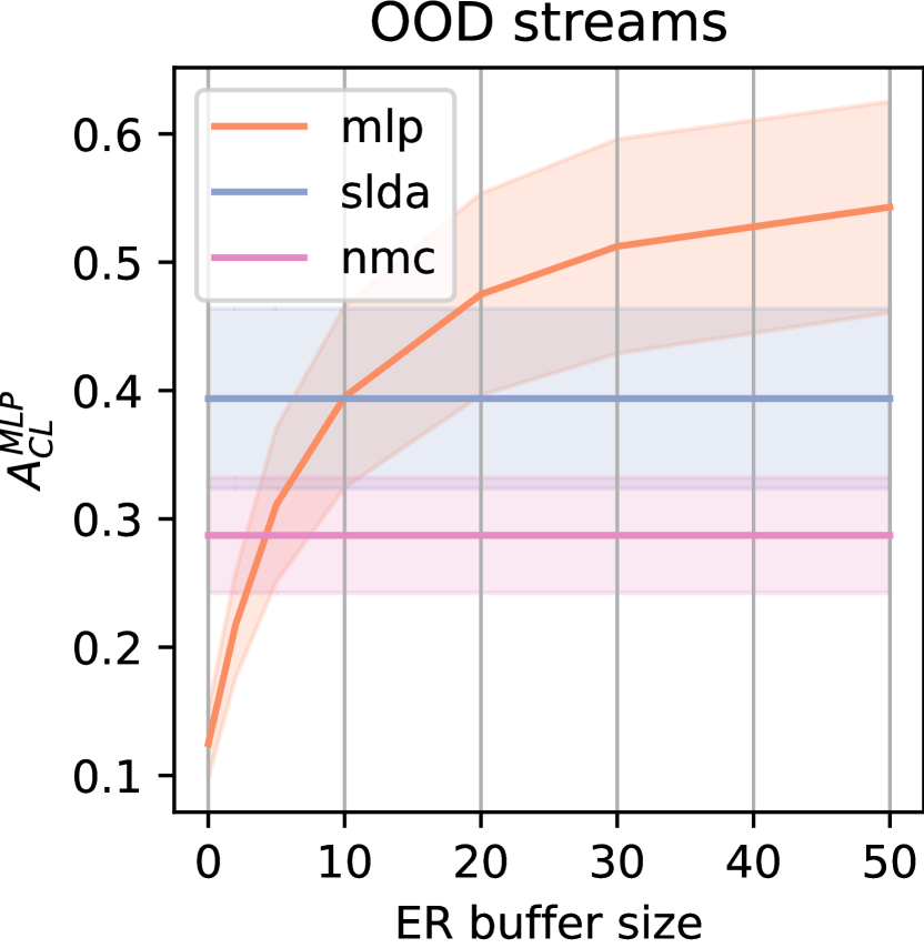
(d) OOD streams

Figure 4: Comparison of metric based accuracy (NMC/SLDA) with the latent ER based solution. This Fig. enables the estimation of the effective replay buffer size of metric-based methods in ID and OOD datasets. Effective buffer size corresponds to the point at which latent ER methods reach the accuracy of SLDA and NMC. It also shows that increasing the buffer size saturates faster the accuracy in ID datasets than on OOD datasets.

Metric based classifiers are compute-efficient and accurate on the ID streams.

In Fig. 4 we compare the performance of the metric based NMC and SLDA classifiers and latent ER based classifiers on both ID and OOD streams. We observe that on the ID streams metric based classifiers achieve superior performance than latent ER ones with small ER size (2 samples per class) and are close to the performance of MLP with large ER buffer (50 samples per class). We can quantify the efficacy of metric based classifiers in terms of effective replay buffer size. As visualized in Fig. 4, effective replay size is the buffer size required by latent ER based methods to reach the accuracy of SLDA and NMC. For latent ER based MLP performance gains beyond this point seem to be very marginal on the ID streams. This highlights the efficacy of the metric based classifiers on the ID streams. This can be attributed to the phenomenon discussed by Papyan et al. (2020) and Galanti et al. (2021), who point out that supervised pre-training can lead to features collapsing to the mean feature vector of the same classes facilitating the applicability of linear and metric based classifiers.

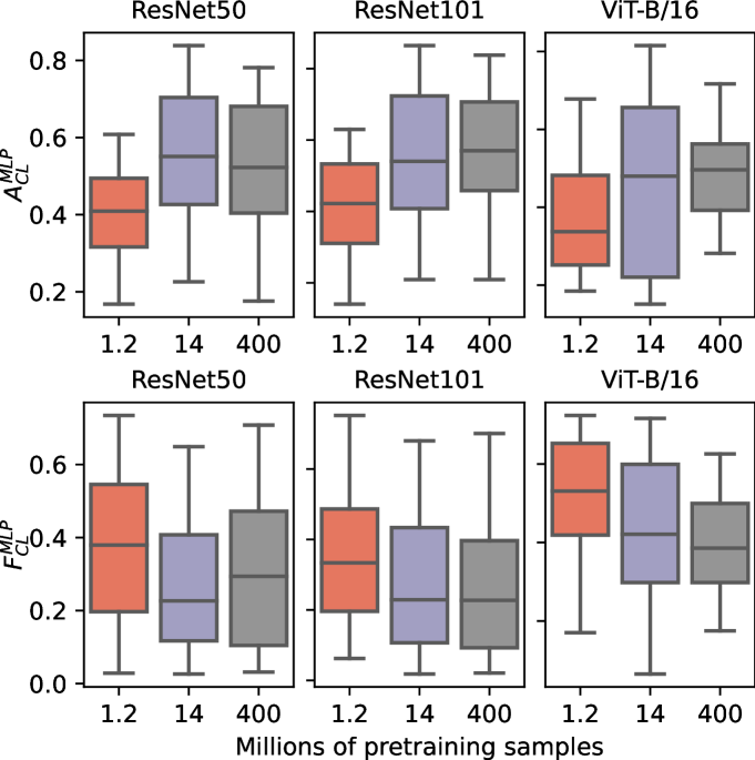
Figure 5: Accuracy ($\uparrow$) and forgetting ($\downarrow$) for three different architecture families (resnet50, resnet101 and ViT) pretrained on different datasets (6 replay buffer sizes, 4 streams and 5 task orders). Here, ResNetV2 (Szegedy et al., 2017) architecture is used for ImageNet21K (14M) dataset, which is slightly different from the standard ResNet architecture. More pre-training data increases CL performance.

All in all, it can be concluded that given a pre-trained encoder that produces “good” representations, CL can be tackled with a non-parametric classifier. Such models are very cheap computationally (see discussion in Appendix C) as they only require single path through the data and no replay. Currently available foundation models provide good representations for some data streams (ID streams) resulting in performance comparable to the more powerful MLP. Additionally, the efficacy of such strategy was demonstrated recently by Banayeeanzade et al. (2021), who first meta-pretrained an encoder and subsequently used a non-parametric classifier to continually learn unseen classes sampled from the same underlying data distribution as the pre-training tasks. While meta-pretraining can be prohibitively expensive on large-scale (Ji et al., 2020), we believe that development of more universal feature encoders, i.e. foundation models pre-trained on broader data distributions, as well as domain-specific pre-training in cases where CL domain is know a priori, will grow the chances of downstream data to be in-distribution easing the CL application.

4.2 Data analysis: pre-training and downstream

Broader pre-training improves latent CL.

Intuitively, pre-training on a broader and more diverse set of examples should improve the universality of the representations produced by a feature extractor (Kaplan et al., 2020; Yuan et al., 2021). We confirm this intuition in Fig. 5, where we depict forgetting and CL accuracy of different architectural families after pre-training on datasets of different sizes. As discussed by  Ridnik et al. (2021) and  Radford et al. (2021) for the datasets used in this study the number of samples can be used as an approximation for the diversity of the pre-training data. As shown in Fig. 5, pre-training on the CLIP dataset (400M examples) tends to produce better results on both large architectural families (ResNet101 and ViT). Interestingly, CLIP models are slightly outperformed by ImageNet21K (14M) pre-trained models in case of ResNet50 architecture. We hypothesize that this is due to limited capacity of the ResNet50 models that is unable to accommodate the diversity of 400M samples.

Similar tasks are harder to learn continually.

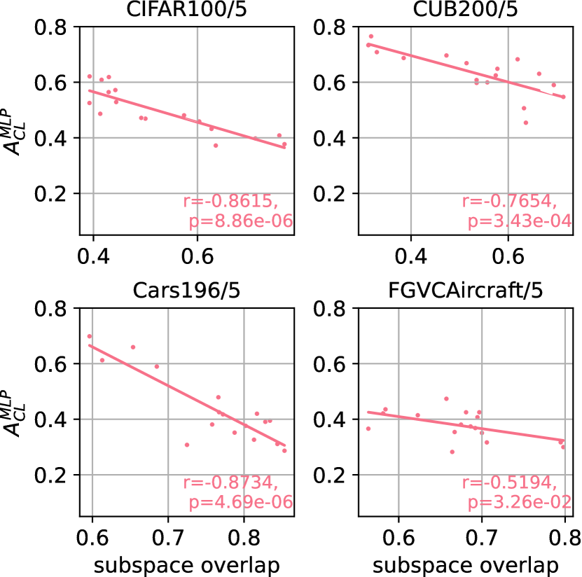
Figure 19: Average Subspace Overlap (Similarity) vs CL Forgetting for multiple datasets where each point represents a pre-trained model averaged over replay sizes and task orders. Overlap correlates negatively with the CL accuracy.

In Fig. 7, we show that class representations in the ID data streams tend to be less similar to each other than class representations from the fine-grained OOD streams (for both similarity metrics). In the cosine similarity measurement, lower similarity is equivalent to more orthogonal class-representations. First, this indicates that ID streams are easier to solve since orthogonal representations are easier to discriminate. This is reflected in the overall higher classification accuracy achieved on the ID streams as shown in Fig. 4. Second, as discussed by Ramasesh et al. (2020), orthogonal representations lead to less forgetting due to less interference. We demonstrate this in Fig. 7, where we plot the subset overlap similarity against $A_{MLP}^{CL}$ (see Sec. 3.3 for details). We can observe a clear negative correlation between CL accuracy and subspace overlap (see Fig. 19 for similar plot but with forgetting and Fig. 19 with interference), i.e. higher subspace overlap correlates with lower CL performance.

Simpler tasks are easier to retain.

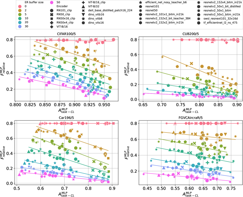
Figure 28: Mean task accuracy (x-axis) vs. relative forgetting (y-axis). Two measurements are well correlated, yet more especially for small replay buffer sizes similar mean task accuracy does not seem to explain forgetting.

In order to better understand the forgetting dynamics, we fit a linear regression to predict forgetting using different variables of interest as predictors, namely the per task accuracy of an MLP, $A_{tasks-iid}^{MLP}$, per task accuracy of SLDA, $A_{tasks-iid}^{SLDA}$, as well as the per task few-shot accuracy $A_{tasks-FS}^{MLP}$. Both $A_{tasks-iid}^{SLDA}$ and $A_{tasks-FS}^{MLP}$ describe the notion of tasks simplicity from two different perspectives: a simple task in the few-shot sense is one for which few examples provide enough information to a non-linear classifier for solving it (few examples + complex model); on the other hand, a task can be simple if a simpler model (SLDA) can fit it well with many samples (many examples + simple model). We plot the $R^{2}$ coefficient of the resulting regressions for different replay buffer sizes in Fig. 5. We observe that few-shot and SLDA accuracy can explain forgetting better (higher $R^{2}$) than $A_{tasks-iid}^{MLP}$ in the low replay buffer regime – i.e. in this regime two models can have a similar ability to learn the downstream tasks ($A_{tasks-iid}^{MLP}$), but very different forgetting behaviour. For example, in Fig. 28 we observe that ViT-B/32 and dino_vitb8 on CIFAR100/5 (ER=2) differ by over 20% points in forgetting but achieve a comparable accuracy on each of the downstream tasks, i.e. have similar $A_{tasks-iid}^{MLP}$. Somewhat unsurprisingly, we conclude that tasks that are simple in the few-shot sense are easier to retain, i.e. need less replay samples. As expected, for larger replay buffers mean task accuracy becomes better at explaining forgetting than the few-shot accuracy.

Adding representations from deeper layers can slightly improve performance.

In their recent work, Evci et al. (2022) (Head2Toe) showed that ensembling representations from the intermediate and the output layers of a feature extractor tends to improve performance of a linear probe on the OOD data. Inspired by their results, we are interested whether such strategy can lead to better CL results. In Fig. 9 we show the improvement achieved through ensembling the final output with each of the intermediate layers over using the final layer only (with the ViT-B/16 encoder). Similar to Evci et al. (2022), we show that there always exists a hidden layer ensembling which always leads to a slight improvement of the CL accuracy (e.g. 2.5%-points on FGVCAircraft). Additionally, we observe a higher variance in the result on OOD streams (Cars196, FGVCAircraft). The result presented here is intended to serve as a proof-of-concept and we did not implement exactly the Head2Toe solution, which also uses L2 lasso regularization for feature selection.

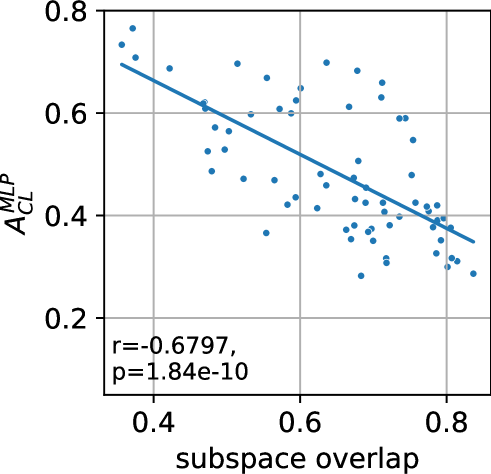
Figure 6: Average Subspace Overlap vs Acc. CL, each point represents a pre-trained model (per stream view in Fig. 19). We also print the Pearson correlation $r$ and $p$-values for completeness. Lower overlap leads to better CL final accuracy.

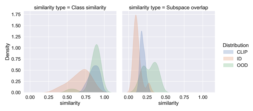
Figure 7: Average similarity density for all our models. (left) with prototypes class cosine similarity. (right) with subspace overlap similarity. We plot separately CLIP’s class similarities since they are not used in the ID vs OOD axis of study. OOD tasks exhibit larger class cos-similarity and more subspace-overlap.

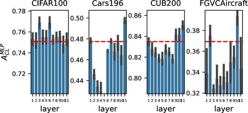
Figure 8: Performance improvement achieved through ensembling deeper and final representations vs. only using final representations (red dotted line). We use ViT-B/16 encoder and ER size of 20 and 5 task orderings. A slight improvement in CL performance can be achieved by adding deeper representations to the input.

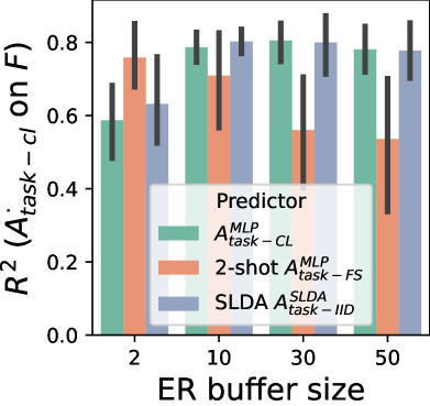
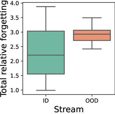
Figure 9: Forgetting analysis.(Left) Coefficient of determination $R^{2}$ ($\uparrow$) of regression fitted to predict forgetting from $A_{tasks-IID}^{MLP}$, $A_{tasks-FS}^{MLP}$ and $A_{tasks-IID}^{SLDA}$. Few-shot performance can better explain forgetting in low replay buffer regime. (Right) Total relative forgetting for ID and OOD streams. There is more forgetting in OOD regime.

Less transfer in OOD streams.

In this section we analyze forward transfer as a function of the input data distribution. We define transfer as the difference of final accuracy between a model trained with and without re-initialization before learning each new task (see Tab. 1). In the presence of replay, positive transfer indicates that some information that was present in the weights of the network was not present in the replay buffer. In Fig. 7b we observe that transfer in OOD streams is significantly higher fthan in ID on average. A possible explanation is that ID data leads to more orthogonality between class prototypes. In this case, few samples from the ER buffer can be more representative of the data distribution of past tasks and no additional information must be stored in the weights of the classifier. In the OOD regime, the replay buffer is less representative of the downstream data due to higher class and task similarity. Weights contain useful information leading to positive transfer. Counter-intuitively, we can conclude that better representation leads to less transfer.

The type of transfer we study here is between the downstream CL tasks. Thereby the tasks are produced through encoding of only four underlying raw data streams with a variety of encoders. Resulting downstream data distributions have substantially different transfer properties as evidenced by the high amount of variance in the transfer result in Fig. 7b. This highlights the strong impact of data distribution properties on the downstream transfer. Studying downstream transfer at this scale in end2end ER regime can have prohibitive computational cost.

More transfer in small replay buffer regime.

In Fig. 7c and 12 we observe that forward transfer is larger in small ER buffer regimes than in the large ER buffer regime. Intuitively, larger buffer size makes CL closer to offline training reducing the importance of weight initialization for forgetting. It is likely that similar result can be observed in the end2end ER setting, validating it would be compute intensive and we decided not to do it.

Bigger upstream / downstream distribution shift leads to more interference.

Intuitively, joint learning of multiple tasks can hinder performance on each individual task due to conflicting learning signals. This effect is known as interference (Kanakis et al., 2020; Kokkinos, 2017). We define total interference as the difference between the mean task accuracy when each task is learned separately ($A_{task-iid}$) and an offline setting, in which all tasks are learned together ($A_{iid}$) (cf. Tab. 1). Our results show that total interference is lower in the ID datasets than in the OOD datasets (Fig. 7a). From our earlier conclusion, we can deduce that the influence factor here is the orthogonality of encoded representations: as visualized in Fig. 19 the more orthogonal the representations are (as measured by subspace overlap), the lower is the total interference. In CL, interference is another factor along forgetting that can lead to performance decrease. It gives us insight into how much the accuracy on each of the downstream tasks is sacrificed in order to remember previous tasks through replay. In Fig. 7d we visualize this relationship by plotting the interference per replay buffer size. i.e. $A_{task-iid}-A_{task-cl}$. We observe that interference is significantly larger when more samples are replayed. Intuitively, more replay makes learning new tasks harder.

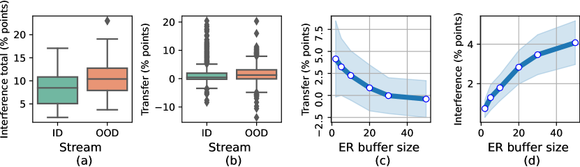
Figure 10: Interference and transfer. (a) Interference total ($\downarrow$) in ID and OOD streams. (b) Forward transfer ($\uparrow$) in ID and OOD streams.(c) Forward transfer ($\uparrow$) per ER size. (d) Interference ($\downarrow$) per replay buffer size. Transfer is larger for small ER sizes and in OOD regime. Interference is bigger in OOD regime and larger ER buffer sizes.

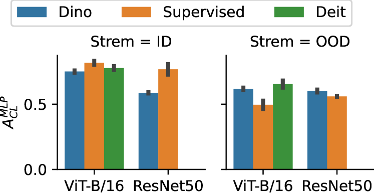
Figure 11: Final CL accuracy of supervised (ImageNet21k), semi-supervised Dino (Caron et al., 2021), and sup.+distillation DeiT (Touvron et al., 2021) pre-training (ImageNet1k). ER buffer size is 50. Per model view in Fig. 25.

4.3 Model level analysis

On encoder universality.

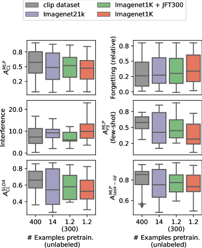
Figure 16: Show the influence of pre-training data regime on the different variables studied. Acc. CL ($\uparrow$), relative forgetting ($\uparrow$), Interference ($\downarrow$), Acc. few-shot, Acc. SLDA and mean task Acc. ($\uparrow$) of models pretrained on different datasets (each boxplot is over 6 replay buffer sizes, 4 streams and 5 task order permutations).

As shown in the appendix Fig. 16, the best performing class of models on average are the CLIP models. This is manifested in the lower forgetting, smaller interference, and, as a result, higher overall $A_{CL}^{MLP}$. While, no encoder dominated the others across all streams, the best performing model is the CLIP ViT-L/14 (2nd largest overall), which is amongst the top-4 best models on all streams as seen in Fig. 25.

Pre-trained encoders encode complementary information.

Given varying efficacy of different model families on different streams, an appealing solution could be to use representation ensembling across models. This is motivated by the success of representation ensembling across layers for better OOD generalization(see Sec. 4.2), and across different views of the same image (Ashukha et al., 2021) to improve ImageNet performance. Here, we concatenate the representations of several encoders and perform CL with latent ER on top. We validate the efficacy of such solution on the multi-dataset stream in Fig. 12. This scenario is especially suitable for evaluating representation ensembling as it contains each of the datasets used to create single-dataset streams, hence the best performing model on this stream should perform reasonably well on the single-dataset streams as well. As shown in Fig. 12, the best performing ensembling model outperforms the best single encoder model by 10% points for the replay buffer size of 2, yet only by approximately 0.8% points for replay buffer size of 30.

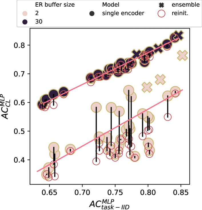
Figure 12: $A_{task-IID}^{MLP}$ vs. $A_{CL}^{MLP}$ on multi-dataset stream. Hollow red points – MLP classifier with ER re-initialized before each new task. Vertical lines show forward transfer. Crosses – ensembled representations. We consider 2 and 30 ER samples per-class on a single task ordering. Detailed view in Fig. 24.

It is worth mentioning that we did not investigate in detail which encoders are most suitable for ensembling of representations (see details in Fig 23) and leave this exploration for future work.

The role of pre-training regime.

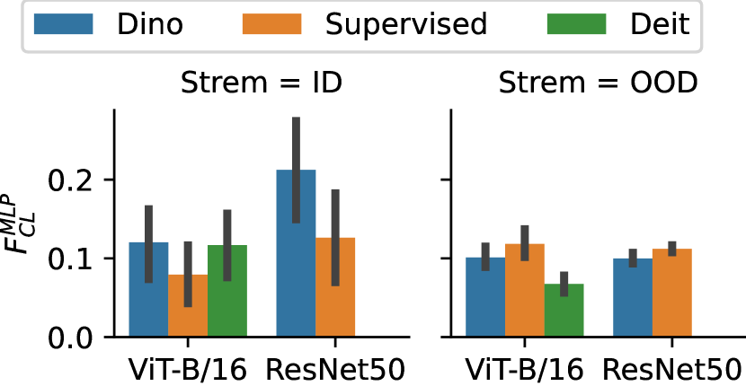
(a) Forgetting

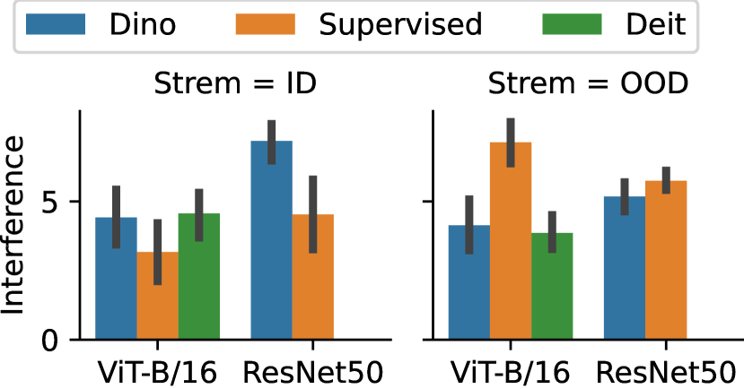
(b) Interference

Figure 29: Forgetting (a) and interference (b) after supervised (ImageNet21K) vs. SSL (dino by Caron et al. [2021], ImageNet1K) and upervised+ditillation (deit by Touvron et al. [2021] based pre-training. Here we compare dino_vitb16, ViT-B/16 and deit_base_distilled_patch16_224, as well as dino_resnet50 and resnetv2_50x1_bitm_in21k models with ER buffer 50.

Encoders used in this paper were pre-trained in supervised, self-supervised (SSL), the mixture of both, supervised with distillation and multimodal (CLIP) regimes (see Tab 2). First, as shown in Fig. 11, we observe that semi-supervised dino (Caron et al., 2021) encoders outperformed ImageNet21K pretrained supervised counterparts on the fine-grained OOD tasks despite having been pretrained on a much smaller ImageNet1K dataset (same holds for interference and forgetting, see Fig 29). This can be attributed to the intuition that supervised pre-training learns features needed to discriminate classes in the pre-training dataset (e.g. higher level classes cars vs. planes) which leads to the phenomenon of neural collapse (Galanti et al., 2021; Papyan et al., 2020) – i.e. features of same classes center around its mean feature vector. This leads to the inability of supervised models to generalize to fine-grained OOD streams. SSL regime does not suffer from model collapse and is able to learn richer features resulting in better OOD performance. Interestingly, similar observation is made for the deit encoder (Touvron et al., 2021), which was pretrained on Imagenet1K dataset using student-teacher distillation. This result extends the observation made by Gallardo et al. (2021) that SSL pre-training is beneficial for CL especially when number of pre-training samples is small, in that we show that it also depends on relation between the pre-training and the downstream tasks.

Some additional indicators

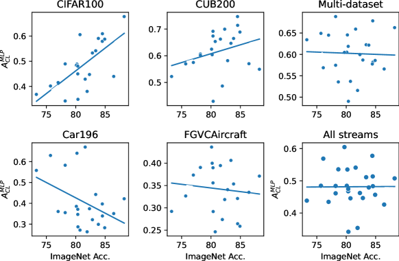
Figure 15: ImageNet accuracy of the encoder (x-axis) and downstream accuracy CL (y-axis). We find positive correlation of the ImageNet accuracy with the downstream CL accuracy for the both in-distribution datasets and slightly negative correlation for the OOD datasets. Overall, however, there is no clear correlation between the two variables. Each point corresponds to a particular, with its CL accuracy averaged over replay buffer sizes (5) and task order permutations(5).

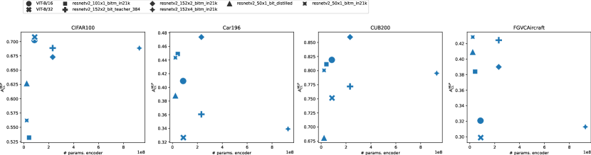
(a) ImageNet21k pretrained models

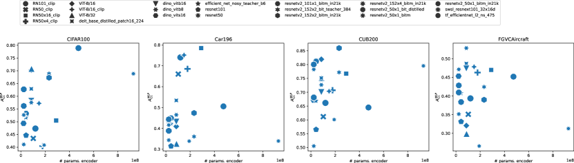
(b) All models

Figure 21: Number of parameters in the encoder (x-axis) vs. CL accuracy (y-axis). No clear correlation can be observed.

that we explored did not show clear correlation with CL performance. These include the size of latent dimension (see Fig.23), the number of parameters in the encoder (see Fig. 21). As for the the accuracy of the encoder on the ImageNet1K dataset it positively correlates with CL performance on the ID datasets and rather negatively on the OOD data streams (see Fig.15).

5 Discussion

Actionability of variables.

In this work, we study a number of characteristics of pretrained models in CL. Notably, we analyze various variables (e.g. Tab 1) that could explain the final CL performance for a given scenario and pretrained model. Those variables have different levels of actionability in practice, i.e. not all of them can help to make informed decisions to maximize future performance in the same way. For instance, some variables are known before accessing the downstream data, e.g. model size, latent dimension size, pre-training FLOPS and pre-training data. This a priori knowledge is highly actionable as it allows selecting models in advance. In our study we found that the influence of the pre-training data overshadows the other variables. In particular, the closeness of pre-training data with downstream data.

On the other hand, in line with Douillard et al. (2020b), we found that getting access to some information about the downstream tasks a priori can help to improve our predictions about downstream performance. We found that the data distribution shift between pre-training and downstream tasks is the most critical factor. For example, with some meta-knowledge about the downstream task such as its domain, we could select a pretrained model trained on a similar domain to minimize the distribution shift. If in-distribution, we found that a few-shot model is a good predictor of downstream performance. Interestingly, we found that it is possible to find if downstream data is in- or out- of distribution without any access to pre-training data using class similarity of downstream embeddings(see Fig. 7). Without access to information before training, we can still use low compute classifiers such as NMC or SLDA on the first batches of data, to have a fast insight of the most suited encoder for a given scenario.

Continual Learning as a function of data.

Instead of studying how various algorithms work on a given dataset, we fix the algorithm and changed the data distribution by changing the encoder. This approach allows to analyze CL while varying the input streams (data perspective ), while in the literature, CL is mostly analyzed from the algorithmic perspective (Lange et al., 2019; Belouadah et al., 2021). In other words, instead of studying various algorithms on a normalized benchmark, we use a normalized algorithm that we study on various benchmarks. Our findings on transfer and interference show that data characteristics can be determinant for CL (cf Section 4.2). We believe that understanding the data characteristics better could significantly improve CL performance and help develop ad-hoc approaches.

A new playground for CL.

By using the pretrained encoders along with existing datasets we were able to generate easy-to-use datasets to prototype and analyze CL algorithms. The encoded datasets are of high diversity, in part because they are created with encoders pretrained in diverse ways and on diverse datasets. Moreover, the inter-class and inter-task similarity of representation in the generated datasets varies significantly as shown in Fig. 7, Fig. 14. The variability of the CL results across encoders and classifiers (MLP, NMC, SLDA) is also a good indicator of encoded dataset diversity. This diverse set of datasets can be used for further research in CL at a significantly lower cost than end-to-end training on raw data. It does not mean that experimentation should not be done in an end-to-end setting. However, using encoded data is a good intermediate state between training a toy datasets such as MNIST and training on dataset that needs a huge amount of compute such as the ones we used as raw data. It is probable that most conclusions in computationally-demanding scenarios can also be made with a lower amount of compute with a diversified set of scenarios, as it was shown to be for reinforcement learning (Ceron and Castro, 2021).

Besides class-incremental learning, the CL stream creation strategy used in this study can also be used for domain-incremental experimentation, for example, by creating a sequence of tasks with the same raw-dataset encoded with various encoders to simulate a representation drift (Caccia and Pineau, 2021; Lesort et al., 2021b).

6 Conclusion

This paper conducts an extensive empirical evaluation of CL on top of foundation models. We show how latent ER is more compute-efficient than end2end ER and when this compute efficiency can be achieved. Additionally, we show that pre-training on broader data results in a representation space with properties favorable for downstream CL. In the extreme case this can allow reduction of CL to training a non-parameteric model on top of encoded features which can have a negligible computational cost and does not require replay by design. This is important because it has the potential to side-step the problem of continual representation learning in some applications. We shed some light on the question of how far are we from this extreme case. It can be concluded that whether we can side-step CL of representations mainly depends on the relation between downstream and upstream data: trivially, if the downstream data distribution was covered in the pre-training, the model is more likely to produce useful features for the downstream tasks, and a non-parameteric model can perform well in the CL phase. Development of foundation models with always better generalization abilities brings us ever closer to such an extreme scenario. However, taking a more nuanced perspective, there is a risk that scaling model pre-training can become computationally unsustainable, and, as discussed by Jang et al. (2021), foundation models can suffer from their knowledge base becoming outdated. Therefore, an interesting future direction could be the development of algorithms for continual refinement of foundation models. Last but not least, this study points out several promising research directions to further improve the efficacy of latent ER in the short term. This includes ensembling of representations coming from different encoders and from the same encoder but different depth.

Appendix

Appendix A Detailed Motivation for Latent ER

Potential of latent ER

With the fast development of foundation models and their effectiveness across tasks and domains, latent CL becomes a more and more appealing alternative to the end2end fine-tuning. This is due to (a) CL time compute advantage enabling per-task hyperparameter search and fast on-device training, (b) potential to improve privacy since storing latent representations of a privacy-preserving model [Xu et al., 2021] for replay may be more secure than storing raw data, as well as (c) better data efficiency since latent representations contain less task-irrelevant information such as pixel noise [Saxe et al., 2019]. (d) As we discuss in the main paper, latent CL can be reduced to training a non-parametric model on top of encoded data, which would solve several long standing problems of CL such as task inference [van de Ven and Tolias, 2019], and could relegate replay as a method of choice for CL, as non-parametric models do not require replay by design [Banayeeanzade et al., 2021]. In this paper we shed some light on the question of how far are we from the extreme case described above. All in all, given the high potential impact of foundation models on the field of CL we believe that the insights provided in this paper are of high relevance for the CL community.

Applicability of latent ER

Continual learning in the latent space is akin to using the encoding procedure as a data pre-processing step. In Section 4.1, we have seen that this methodology can produce representations that outperform raw data in terms of CL performance and computation. To succeed, latent ER should encode class discriminative information as good as it is encoded in the the raw data (i.e. no task-relevant information is destroyed). This can be true in at least two cases: either the pre-training domain is similar to the downstream CL domain (Figure 2), or the pre-training domain is extremely broad (Figure 5), such that the produced representations are likely to work with any domain encountered in the CL phase. An example of the first case is a situation in which the CL domain is known a priori, such as pre-training a feature encoder for self-driving applications. The latter case is addressed through the development of foundation models [Radford et al., 2021, Bommasani et al., 2021]. It is important to highlight that the goal of foundation models is specifically the creation of models effective across wide range of tasks and domains, i.e. models for which all downstream tasks will be ID. This makes latent ER an increasingly promising strategy for CL.

Appendix B Latent ER vs. end2end ER

We calculate number of flops required by the models using the fvcore library. Thereby the computational cost of a backward path is roughly twice as large as the computation cost of the forward path. . Unless otherwise stated, when estimating the computational cost of latent ER models, we take into account the encoding cost, that is the cost of forward passing each sample through the encoder one time.

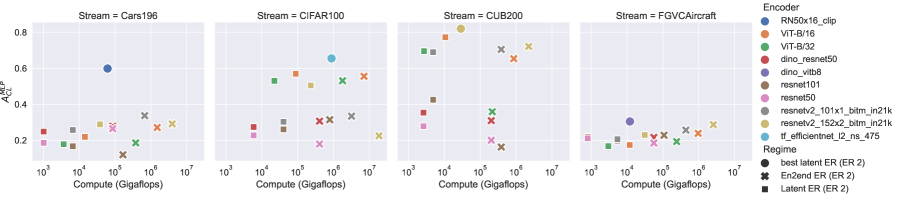
(a) ER buffer size 2

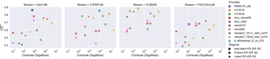
(b) ER buffer size 30

Figure 13: Compute-accuracy trade-off of raw data ER (end2end) vs. latent ER models. We plot 7 different models in both end2end ER and latent ER regime on 4 streams and using 2 ER buffer sizes (2 and 30 samples per class). Additionally, we plot the best latent ER model for each stream (e.g. dino_vitb8 model in the FGVCAircraft stream) End2end ER leads to performance improvement on the OOD streams (Cars196 and FGVCAircraft) at the expense of more compute. The best performing latent ER model outperforms or reaches comparable accuracy of the best end2end ER model on all streams.

Appendix C Computational cost of metric based models

Metric-based models used in this paper use statistics of data to classify them. Hence, the nearest mean classifier computes the mean of features of each class and looks for the closest ( $L_{2}$ norm ) mean to classify a new data point. When the feature encoder is frozen the full compute cost of NMC is then: $C_{enc}*Card(\mathbb{D})+Card(\mathbb{D})*N_{z}+N_{z}*N_{c}$ With $C_{enc}$ the number of flops to encode one image, $Card(\mathbb{D})$ the number of sample in the dataset/task $\mathbb{D}$, $N_{z}$ the latent dimension size and $N_{c}$. $Card(\mathbb{D})*N_{z}$ correspond in summing all latent vectors and $N_{z}*N_{c}$ to normalize vectors for each class.

The SLDA approach is more compute consuming since it needs to compute means and covariance matrice but also because it needs to invert the covariance matrix for inference. The covariance matrix is a $N_{z}\times N_{z}$ matrix computed such as:

$$cov(z_{i},z_{j})=\mathbb{E}[(z_{i}-\mathbb{E}[z_{i}])(z_{j}-\mathbb{E}[z_{j}])]$$ (1)

With $z_{i}$ the dimension $i\in[0,N_{z}-1]$ of the latent representation. Assuming $\mathbb{E}[z_{i}]$ and $\mathbb{E}[z_{i}]$ already computed while estimating the mean of classes. The compute cost for the full matrix $\Sigma$ is: $(3*N_{z}\times\mathbb{D})^{2}$. The inversion of a matrice has a complexity of $O(n^{3})$, so we can roughly estimate the compute to be similar to ${N_{z}}^{3}$ flops to invert the covariance matrice. The total compute of SLDA is then roughly: $C_{enc}*Card(\mathbb{D})+Card(\mathbb{D})*N_{z}+N_{z}*N_{c}+(3*N_{z}\times\mathbb{D})^{2}+{N_{z}}^{3}$. With a large latent dimension, the biggest cost of SLDA is the covariance matrix inversion. Hence depending on the representation size SLDA might be more or less computed efficiently. For example, with our biggest representation size (8192 resnetv2-152x4-bitm), the matrix inversion is around $5.5\times 10^{2}$ gigaflops which is still lower than latent replay compute (cf Figure 11) but several order of magnitude bigger than NMC.

Appendix D Task and class similarity

Subspace overlap measures the average task similarity of a sequence by comparing the orthogonal sub spaces of each task with each other task. If $n$ distinct tasks are represented by their centered latent representations $(t_{1},t_{2},...,t_{n})$ in a sequence and $t_{i}\in R^{p\times q}$, $p$ is the number of samples and $q$ is the latent dimension:

$$Overlap_{avg}=\frac{1}{T}\sum_{i=1}^{n}\sum_{j=i+1}^{n}Overlap_{subs}(t_{i},t_{j}),$$ (2)

Here, $T$ is the number of pairs, where each task representations are compared with the upcoming ones.

$$Overlap_{subs}(t_{i},t_{j})=\frac{1}{k}\|U_{k}^{T}V_{k}\|^{2}_{F}.$$ (3)

Here, $U_{k}$ be the matrix formed by eigenvectors of $t_{i}^{T}t_{i}$ for top $k$ principal directions and $V_{k}$ be the matrix formed by eigenvectors of $t_{j}^{T}t_{j}$ for top $k$ principal directions. For the subspace similarity analysis, we fix $k=20$, which captures around $56$% of average variance of the latent representations for all the datasets and models.

To measure the class similarities in a sequence, we represent each class by a prototype which is computed by the mean of latent representations of the samples of that class and measure the pairwise cosine similarities. Given $c$ classes, each class is represented by prototypes $(p_{1},p_{2},...,p_{c})$, where each $p_{i}$ is a vector in $R^{q}$. Class similarity is defined as:

$$ClassSim_{avg}=\frac{1}{T}\sum_{i=1}^{c}\sum_{j=i+1}^{c}CosSim(p_{i},p_{j}),$$ (4)

Here, $T$ is the number of possible pairs of prototypes and $CosSim$ is the cosine similarity function.

Appendix E Training details

E.1 Hyperparameters

We perform hyperparameter selection (learning rate, weight decay, and whether to anneal the learning rate) using the validation accuracy. On single dataset splits (e.g. CIFAR100/5) we run hyperparameter selection only on the first task and keep the hyperparameters for the rest of the stream. Unless stated otherwise, we use 5 different randomly selected but fixed task orderings for all experiments. On the multi-dataset stream we perform per-task hyperparameter search. Unless otherwise stated, we average all results over 5 different task orders to factor out results from a particular task order.

E.2 Models

Among the models used 11 are based on transformers [Dosovitskiy et al., 2020, Touvron et al., 2021] and 19 on ResNets [He et al., 2020, Zagoruyko and Komodakis, 2016, Kolesnikov et al., 2020, Tan and Le, 2019]. We use 13 models pre-trained on ImageNet 1k [Deng et al., 2009], 9 on ImageNet 21k [Kolesnikov et al., 2020], 6 on CLIP [Radford et al., 2021], 1 on JFT [Sun et al., 2017] + Imagenet 1k [Tan and Le, 2019], and 1 with 940M of unlabeled images [Yalniz et al., 2019]. From these models, 7 are trained with self-supervision [Caron et al., 2021], 7 are big-transfer models [Kolesnikov et al., 2020], and 1 is trained via semi-weakly supervised learning [Yalniz et al., 2019]. Table 2 contains the specifications of the models used for the empirical study.

Table 2: Pre-trained model details. Encoder indicates the architecture in timm format, Linear indicates whether results were obtained by fine-tuning the model (NO) or by training a linear layer on top of frozen features (YES). Pretraining data contains the dataset used for pre-training. #Examples shows the size of the pre-training datasets. Supervision indicates the type of supervision to train the encoder. Dim is the output latent dimensionality. #Params is the number of parameters of the pre-trained model. Acc is the ImageNet top-1 accuracy of the pre-trained model.

Encoder	Linear	Pretraining data	#Examples	Supervision	Dim	#Params	Acc
RN101_clip	YES	clip dataset	400.0M	text	512	119.7M	75.70
RN50_clip	YES	clip dataset	400.0M	text	1024	102.0M	73.30
RN50x16_clip	YES	clip dataset	400.0M	text	768	291.0M	81.60
RN50x4_clip	YES	clip dataset	400.0M	text	640	178.3M	78.20
ViT-L/14_clip	YES	clip dataset	400.0M	text	768	427M	83.90
RN50x64_clip	YES	clip dataset	400.0M	text	623	623M	83.60
ViT-B/16_clip	YES	clip dataset	400.0M	text	512	149.6M	80.20
ViT-B/32_clip	YES	clip dataset	400.0M	text	512	151.3M	76.10
dino_resnet50	YES	Imagenet1K	1.3M	dino	2048	23.5M	75.30
dino_vitb16	YES	Imagenet1K	1.3M	dino	768	85.8M	78.20
dino_vitb16	NO	Imagenet1K	1.3M	dino	768	85.8M	81.50
dino_vitb8	NO	Imagenet1K	1.3M	dino	768	85.8M	82.80
dino_vitb8	YES	Imagenet1K	1.3M	dino	768	85.8M	80.10
dino_vits16	YES	Imagenet1K	1.3M	dino	384	21.7M	77.00
dino_vits8	YES	Imagenet1K	1.3M	dino	384	21.7M	79.70
ViT-B/16	NO	Imagenet21k	14.2M	labels	768	85.8M	84.53
ViT-B/32	NO	Imagenet21k	14.2M	labels	768	87.5M	80.72
resnet101	NO	Imagenet1K	1.3M	labels	2048	42.5M	81.93
resnet152	NO	Imagenet1K	1.3M	labels	2048	58.1M	78.66
resnet50	NO	Imagenet1K	1.3M	labels	2048	23.5M	80.37
resnetv2_50x1_bitm_in21k	NO	Imagenet21k	14.2M	labels	2048	23.5M	80.34
resnetv2_101x1_bitm_in21k	NO	Imagenet21k	14.2M	labels	2048	42.5M	82.33
resnetv2_101x3_bitm_in21k	NO	Imagenet21k	14.2M	labels	6144	381.8M	84.44
resnetv2_152x2_bit_teacher_384	NO	Imagenet21k	14.2M	labels	4096	232.2M	83.84
resnetv2_152x2_bitm_in21k	NO	Imagenet21k	14.2M	labels	4096	232.2M	84.51
resnetv2_152x4_bitm_in21k	NO	Imagenet21k	14.2M	labels	8192	928.3M	84.92
resnetv2_50x1_bit_distilled	NO	Imagenet21k	14.2M	labels	2048	23.5M	82.83
resnetv2_50x1_bitm	NO	Imagenet1K	1.3M	labels	2048	23.5M	80.34
swsl_resnext101_32x16d	NO	Imagenet1K + Unlabeled	1.3M	labels + semi-supervised	2048	192.0M	83.36
tf_efficientnet_l2_ns_475	NO	Imagenet1K + JFT300	1.3M	labels + semi-supervised	5504	474.8M	88.23
deit_base_distilled_patch16_224	NO	Imagenet1K	1.3M	labels + distillation	768	85.8M	83.39
efficient_net_nosy_teacher_b6	NO	Imagenet1K + JFT300	1.3M	labels + distillation	2304	40.7M	86.45

Appendix F Additional Figures

In this section we include additional figures that are referenced in the main text.

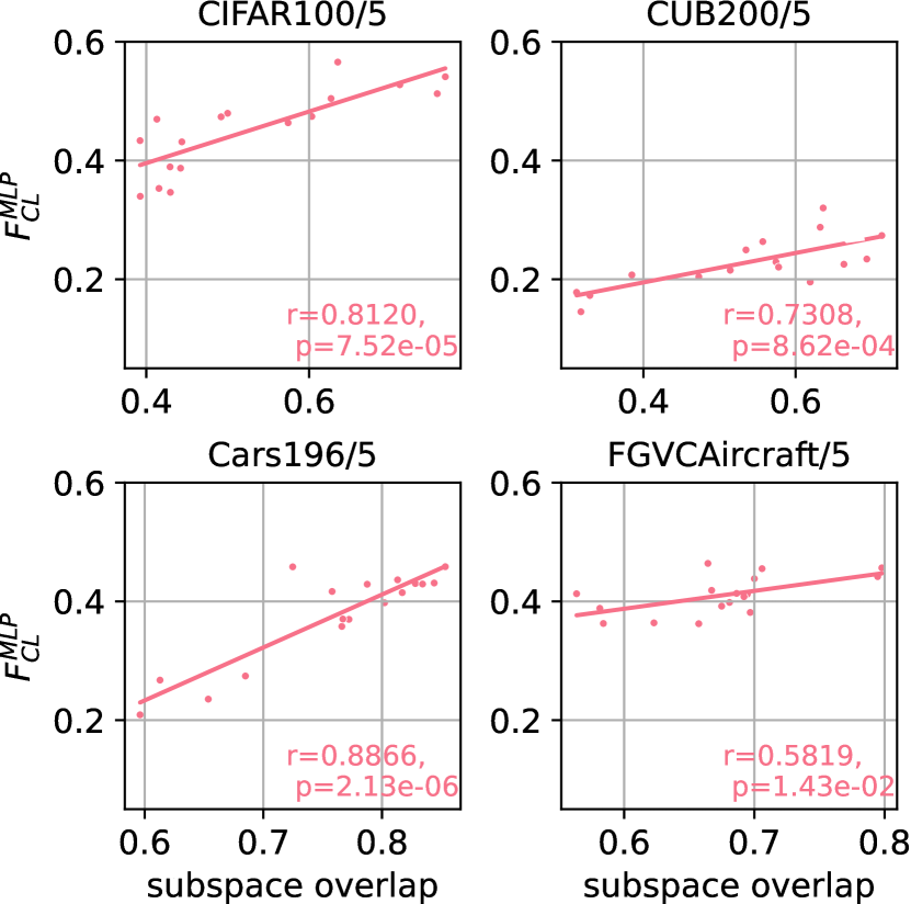
Figure 17: Average Subspace Overlap (Similarity) vs CL Forgetting for multiple datasets where each point represents a pre-trained model averaged over replay sizes and task orders. Overlap correlates negatively with the CL accuracy.

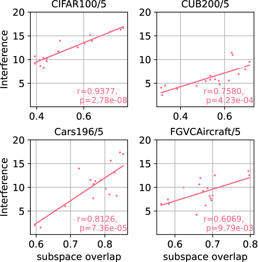
Figure 18: Average Subspace Overlap (Similarity) vs CL interference for multiple data-sets where each point represents a pre-trained model averaged over replay sizes and task orders. Overlap correlates positively with the CL accuracy.

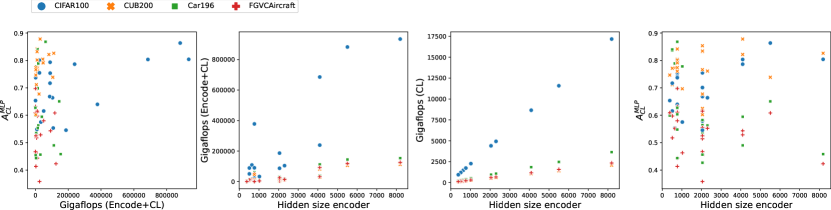
Figure 22: How compute, hidden size and latent dimension of the encoder relate to each other (ER buffer size = 50).

Figure 23: Correlation coefficient between latent size and forgetting (calculated separately for each replay buffer size and averaged). Refer to Fig. 22 for details. Latent dimension does not influence final performance or relative forgetting in our datasets.

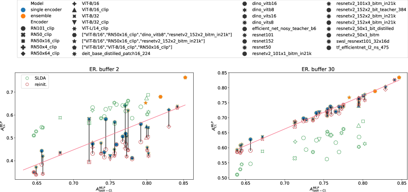
Figure 24: Detailed performance of each mopdel on the multi-dataset stream. Green hollow points correspond to the performance of the SLDA classifier $A_{CL}^{SLDA}$, hollow red – performance of MLP trained with replay but reinitialized before each task, $A_{CL-reinit}^{MLP}$. Green points correspond to the MLP trained with ER, $A_{CL}^{MLP}$. We also include models with ensembled representations (see legend). Remarkably, the best ensembled model with replay buffer size of 2 (76.4%) almost reaches the performance of the third best single model with the replay buffer size of 30 (“dino_vitb8” with 77.7%), with the other two best ones being the largest CLIP models (’RN50x64_clip’ – 80.3% and “ViT-L/14_clip” with 82.6%). Due to long run-time of this experiment we only considered a single task ordering here.

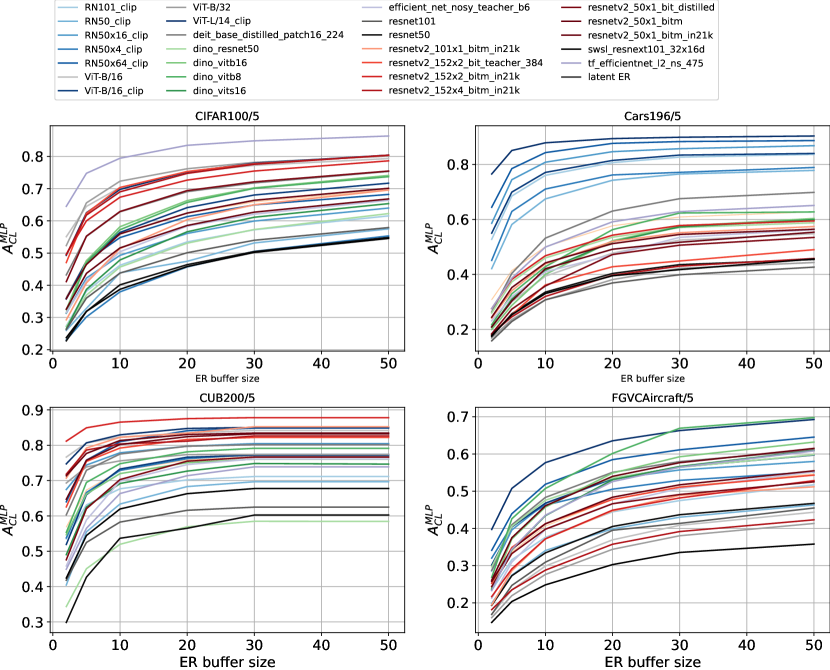
Figure 26: CL performance of various encoders (colors correspond to different encoder families, e.g. blue - CLIP, red – BiT [Kolesnikov et al., 2020] models) for different replay buffer sizes. While all encoders’ performance improves as more samples are added to the replay buffer, there is no model universal that dominates all streams.

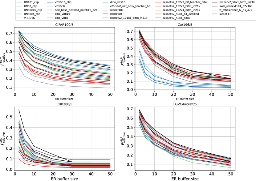
Figure 27: ER buffer efficiency per encoder. Different encoders have different amount of relative forgetting (average amount of accuracy lost after learning the whoel task sequence in %) across the replay buffer sizes.

Appendix G Limitations

In the following we list the limitations of this study.

First, this study only considers one domain, namely the vision domain. We believe similar results are likely to apply in other domains such as Natural Language Processing (NLP). Due to the specifics of the NLP domain, a rigorous evaluation of modern Language Models (LM) would deserve a separate paper on its own and would exceed the scope of this study. For example, one interesting, and NLP-specific question, could be whether and when fine-tuning of LMs is necessary at all, and if simple prompting could lead to good performance on downstream tasks in certain contexts. Additionally, language offers some interesting types of distribution shifts, such as e.g. outdated factual knowledge  [Jang et al., 2021], which deserve a separate discussion. Finally, in the context of NLP, a similar study has been conducted recently by  Wu et al. [2022], however this study does not consider baselines with completely fixed encoders.

Another limitation is that we solely focus on replay strategy and class-incremental scenario. This choice is motivated by the generality of the replay strategy as it can be applicable in most CL scenarios [Kalifou et al., 2019, Diethe et al., 2018, Lesort et al., 2019, Prabhu et al., 2020, Traoré et al., 2019, Belouadah and Popescu, 2018, Wu et al., 2019, Hou et al., 2019, Lesort, 2020, Douillard et al., 2020a].

Finally, the variance (for a single experimental setup) in our study comes from different task orderings and not from varying the seed of the classifier. initialization. Varying the seed would not affect the encoding procedure while it would significantly increase the number of experiments. Additionally, the classifier is usually not reinitialised before each task, hence changing the seed would effect only the classifier initialisation before learning the whole stream. At the same time changing the task ordering actually effects the state of the classifier throughout the stream.

Appendix H Detailed list of results

Tab. H and Tab. H contains a detailed list of results for multiple models and datasets with replay size of 2 and 50, averaged over 5 different task orders.

Table 3: Baseline results on replay size of 2 averaged over 5 tasks order.

Dataset	Encoder	MLP	reinit	NMC	SLDA	upperbound	FSH	transfer	interference
CIFAR100	RN101-clip	$27.36$$\pm 0.62$	$25.38$$\pm 0.55$	$56.04$$\pm 0.00$	$58.20$$\pm 0.71$	$72.98$$\pm 0.87$	$58.26$$\pm 0.20$	$1.98$$\pm 0.83$	$15.15$$\pm 0.98$
-	RN50-clip	$25.99$$\pm 0.74$	$25.24$$\pm 1.17$	$47.30$$\pm 0.00$	$52.54$$\pm 0.38$	$70.13$$\pm 0.19$	$49.06$$\pm 0.72$	$0.75$$\pm 1.46$	$15.85$$\pm 0.44$
-	RN50x16-clip	$31.30$$\pm 0.76$	$30.54$$\pm 0.89$	$57.00$$\pm 0.00$	$61.33$$\pm 0.61$	$75.31$$\pm 0.14$	$54.12$$\pm 0.29$	$0.76$$\pm 0.70$	$13.40$$\pm 0.21$
-	RN50x4-clip	$23.01$$\pm 0.91$	$22.44$$\pm 0.70$	$53.75$$\pm 0.00$	$57.76$$\pm 0.44$	$73.45$$\pm 0.12$	$53.17$$\pm 0.82$	$0.57$$\pm 0.88$	$13.90$$\pm 0.12$
-	RN50x64-clip	$35.97$$\pm 1.14$	$29.04$$\pm 1.45$	$60.68$$\pm 0.00$	$66.97$$\pm 0.51$	$78.58$$\pm 0.09$	$53.75$$\pm 0.60$	$6.93$$\pm 0.64$	$12.34$$\pm 0.17$
-	ViT-B/16	$55.09$$\pm 1.10$	$46.82$$\pm 1.27$	$81.39$$\pm 0.00$	$79.89$$\pm 0.25$	$85.59$$\pm 0.16$	$84.86$$\pm 0.07$	$8.26$$\pm 1.31$	$8.24$$\pm 0.12$
-	ViT-B/16-clip	$35.74$$\pm 1.09$	$32.45$$\pm 2.13$	$69.91$$\pm 0.00$	$71.70$$\pm 0.24$	$82.27$$\pm 0.09$	$68.76$$\pm 0.17$	$3.29$$\pm 2.47$	$10.21$$\pm 0.16$
-	ViT-B/32	$52.32$$\pm 1.38$	$52.38$$\pm 1.51$	$80.29$$\pm 0.00$	$78.79$$\pm 0.25$	$84.98$$\pm 0.42$	$83.25$$\pm 0.13$	$-0.05$$\pm 0.17$	$8.69$$\pm 0.39$
-	ViT-L/14-clip	$49.31$$\pm 0.78$	$39.36$$\pm 1.07$	$79.38$$\pm 0.00$	$81.12$$\pm 0.39$	$87.19$$\pm 0.08$	$73.50$$\pm 0.28$	$9.95$$\pm 1.20$	$7.73$$\pm 0.06$
-	deit-base-distilled-patch16-224	$43.21$$\pm 1.03$	$33.05$$\pm 0.42$	$73.75$$\pm 0.00$	$75.52$$\pm 0.17$	$84.42$$\pm 0.13$	$69.00$$\pm 0.52$	$10.16$$\pm 0.66$	$9.69$$\pm 0.16$
-	dino-resnet50	$30.26$$\pm 3.93$	$21.55$$\pm 0.94$	$57.30$$\pm 0.00$	$60.08$$\pm 0.34$	$74.60$$\pm 0.24$	$55.40$$\pm 0.21$	$8.71$$\pm 3.48$	$14.16$$\pm 0.29$
-	dino-vitb16	$32.45$$\pm 0.38$	$32.42$$\pm 0.46$	$73.22$$\pm 0.00$	$73.30$$\pm 0.26$	$82.98$$\pm 0.17$	$65.83$$\pm 1.93$	$0.03$$\pm 0.17$	$10.67$$\pm 0.12$
-	dino-vitb8	$32.19$$\pm 0.41$	$31.97$$\pm 0.51$	$73.00$$\pm 0.00$	$73.57$$\pm 0.24$	$83.46$$\pm 0.19$	$67.75$$\pm 0.98$	$0.22$$\pm 0.39$	$10.22$$\pm 0.24$
-	dino-vits16	$27.79$$\pm 0.81$	$27.50$$\pm 0.70$	$66.19$$\pm 0.00$	$65.48$$\pm 0.29$	$77.44$$\pm 0.31$	$51.05$$\pm 2.09$	$0.29$$\pm 0.26$	$13.97$$\pm 0.42$
-	efficient-net-nosy-teacher-b6	$31.54$$\pm 0.89$	$28.21$$\pm 0.78$	$65.28$$\pm 0.00$	$68.02$$\pm 0.61$	$78.58$$\pm 0.23$	$65.56$$\pm 0.24$	$3.33$$\pm 0.24$	$11.75$$\pm 0.30$
-	resnet101	$26.27$$\pm 0.44$	$25.36$$\pm 0.45$	$54.74$$\pm 0.00$	$55.19$$\pm 0.30$	$68.80$$\pm 0.20$	$57.23$$\pm 0.25$	$0.90$$\pm 0.13$	$16.29$$\pm 0.24$
-	resnet50	$22.75$$\pm 0.69$	$22.88$$\pm 0.46$	$51.43$$\pm 0.00$	$52.66$$\pm 0.52$	$66.98$$\pm 0.27$	$48.19$$\pm 0.69$	$-0.13$$\pm 0.80$	$16.66$$\pm 0.31$
-	resnetv2-101x1-bitm-in21k	$30.09$$\pm 0.66$	$27.64$$\pm 0.32$	$74.32$$\pm 0.00$	$74.61$$\pm 0.20$	$82.86$$\pm 0.16$	$70.94$$\pm 0.33$	$2.45$$\pm 0.64$	$9.95$$\pm 0.13$
-	resnetv2-152x2-bit-teacher-384	$47.06$$\pm 0.89$	$45.61$$\pm 1.12$	$79.22$$\pm 0.00$	$79.08$$\pm 0.16$	$85.60$$\pm 0.10$	$78.59$$\pm 0.31$	$1.45$$\pm 0.27$	$9.15$$\pm 0.06$
-	resnetv2-152x2-bitm-in21k	$49.60$$\pm 3.01$	$36.31$$\pm 2.53$	$79.00$$\pm 0.00$	$79.56$$\pm 0.33$	$86.12$$\pm 0.17$	$74.93$$\pm 0.46$	$13.30$$\pm 1.77$	$8.61$$\pm 0.14$
-	resnetv2-152x4-bitm-in21k	$49.54$$\pm 2.94$	$35.70$$\pm 1.27$	$79.58$$\pm 0.00$	$80.86$$\pm 0.14$	$86.86$$\pm 0.22$	$70.77$$\pm 0.38$	$13.85$$\pm 2.10$	$8.26$$\pm 0.20$
-	resnetv2-50x1-bit-distilled	$41.14$$\pm 1.05$	$41.20$$\pm 0.99$	$71.11$$\pm 0.00$	$72.49$$\pm 0.14$	$83.22$$\pm 0.21$	$73.93$$\pm 0.25$	$-0.06$$\pm 0.14$	$10.34$$\pm 0.17$
-	resnetv2-50x1-bitm	$32.58$$\pm 0.93$	$28.12$$\pm 0.70$	$62.77$$\pm 0.00$	$64.72$$\pm 0.43$	$77.98$$\pm 0.08$	$63.87$$\pm 0.32$	$4.46$$\pm 0.76$	$12.57$$\pm 0.19$
-	resnetv2-50x1-bitm-in21k	$35.85$$\pm 1.55$	$29.16$$\pm 0.92$	$69.56$$\pm 0.00$	$70.33$$\pm 0.52$	$80.40$$\pm 0.17$	$66.84$$\pm 0.54$	$6.69$$\pm 1.08$	$11.45$$\pm 0.23$
-	swsl-resnext101-32x16d	$23.73$$\pm 0.78$	$23.26$$\pm 0.66$	$53.23$$\pm 0.00$	$40.43$$\pm 0.33$	$69.22$$\pm 0.08$	$53.96$$\pm 0.70$	$0.47$$\pm 0.94$	$14.96$$\pm 0.26$
-	tf-efficientnet-l2-ns-475	$64.52$$\pm 1.33$	$63.44$$\pm 2.58$	$83.76$$\pm 0.00$	$84.09$$\pm 0.42$	$90.45$$\pm 0.06$	$88.46$$\pm 0.12$	$1.08$$\pm 2.35$	$6.11$$\pm 0.14$
CUB200	RN101-clip	$53.53$$\pm 1.25$	$44.75$$\pm 1.67$	$69.44$$\pm 0.00$	$62.55$$\pm 0.84$	$72.53$$\pm 0.97$	$56.87$$\pm 0.45$	$8.77$$\pm 0.54$	$7.95$$\pm 0.92$
-	RN50-clip	$40.44$$\pm 1.06$	$38.83$$\pm 0.98$	$60.55$$\pm 0.00$	$56.73$$\pm 1.28$	$69.89$$\pm 0.99$	$50.95$$\pm 0.73$	$1.62$$\pm 0.63$	$9.54$$\pm 1.01$
-	RN50x16-clip	$67.47$$\pm 1.38$	$57.55$$\pm 1.53$	$79.31$$\pm 0.00$	$76.42$$\pm 0.77$	$81.25$$\pm 0.47$	$65.99$$\pm 0.47$	$9.92$$\pm 0.54$	$5.57$$\pm 0.60$
-	RN50x4-clip	$53.79$$\pm 1.94$	$51.99$$\pm 1.90$	$74.52$$\pm 0.00$	$68.87$$\pm 0.76$	$76.99$$\pm 0.23$	$61.86$$\pm 0.54$	$1.80$$\pm 0.64$	$6.93$$\pm 0.44$
-	RN50x64-clip	$63.98$$\pm 1.53$	$62.26$$\pm 1.49$	$80.81$$\pm 0.00$	$80.37$$\pm 0.35$	$85.38$$\pm 0.33$	$70.11$$\pm 0.30$	$1.73$$\pm 0.54$	$3.38$$\pm 0.60$
-	ViT-B/16	$76.64$$\pm 1.60$	$70.66$$\pm 1.42$	$80.57$$\pm 0.00$	$80.69$$\pm 0.36$	$84.04$$\pm 0.73$	$74.28$$\pm 1.48$	$5.99$$\pm 0.27$	$3.15$$\pm 0.60$
-	ViT-B/16-clip	$51.92$$\pm 2.09$	$51.80$$\pm 1.97$	$76.09$$\pm 0.00$	$71.03$$\pm 0.73$	$79.83$$\pm 0.22$	$64.49$$\pm 0.55$	$0.11$$\pm 1.23$	$6.18$$\pm 0.28$
-	ViT-B/32	$69.31$$\pm 0.86$	$62.86$$\pm 1.59$	$74.60$$\pm 0.00$	$73.69$$\pm 0.34$	$78.58$$\pm 0.08$	$71.21$$\pm 0.25$	$6.45$$\pm 0.99$	$4.86$$\pm 0.15$
-	ViT-L/14-clip	$74.73$$\pm 1.68$	$64.98$$\pm 1.63$	$82.47$$\pm 0.00$	$80.94$$\pm 0.73$	$85.32$$\pm 0.26$	$71.69$$\pm 0.32$	$9.76$$\pm 0.90$	$4.27$$\pm 0.40$
-	deit-base-distilled-patch16-224	$60.31$$\pm 1.36$	$52.69$$\pm 1.87$	$76.82$$\pm 0.00$	$76.71$$\pm 0.64$	$81.15$$\pm 0.58$	$63.24$$\pm 0.55$	$7.62$$\pm 1.00$	$5.46$$\pm 0.46$
-	dino-resnet50	$34.52$$\pm 0.84$	$22.77$$\pm 0.77$	$31.94$$\pm 0.00$	$42.51$$\pm 0.82$	$60.33$$\pm 0.45$	$27.98$$\pm 0.61$	$11.74$$\pm 0.51$	$9.46$$\pm 0.69$
-	dino-vitb16	$54.67$$\pm 1.19$	$37.89$$\pm 1.26$	$62.25$$\pm 0.00$	$67.06$$\pm 0.44$	$76.82$$\pm 0.55$	$46.49$$\pm 0.69$	$16.78$$\pm 0.88$	$5.51$$\pm 0.71$
-	dino-vitb8	$55.34$$\pm 3.04$	$37.90$$\pm 1.38$	$58.41$$\pm 0.00$	$68.09$$\pm 0.24$	$79.23$$\pm 0.72$	$44.57$$\pm 1.37$	$17.43$$\pm 3.76$	$4.75$$\pm 0.75$
-	dino-vits16	$49.02$$\pm 1.76$	$42.38$$\pm 1.38$	$69.43$$\pm 0.00$	$68.16$$\pm 0.71$	$77.57$$\pm 0.84$	$53.48$$\pm 2.09$	$6.64$$\pm 1.02$	$5.83$$\pm 1.11$
-	efficient-net-nosy-teacher-b6	$45.82$$\pm 2.07$	$44.18$$\pm 1.22$	$63.02$$\pm 0.00$	$70.33$$\pm 0.77$	$77.84$$\pm 0.20$	$52.13$$\pm 0.49$	$1.64$$\pm 2.30$	$5.75$$\pm 0.18$
-	resnet101	$41.78$$\pm 1.48$	$33.32$$\pm 1.38$	$58.48$$\pm 0.00$	$55.76$$\pm 0.49$	$63.88$$\pm 1.40$	$48.67$$\pm 0.50$	$8.47$$\pm 0.33$	$11.45$$\pm 1.30$
-	resnet50	$29.85$$\pm 2.22$	$29.43$$\pm 2.39$	$56.00$$\pm 0.00$	$53.16$$\pm 0.59$	$62.12$$\pm 0.55$	$44.68$$\pm 0.49$	$0.42$$\pm 1.93$	$10.97$$\pm 0.76$
-	resnetv2-101x1-bitm-in21k	$74.49$$\pm 1.50$	$70.23$$\pm 1.08$	$84.23$$\pm 0.00$	$84.21$$\pm 0.37$	$86.18$$\pm 0.72$	$76.07$$\pm 1.07$	$4.27$$\pm 1.43$	$4.07$$\pm 0.76$
-	resnetv2-152x2-bit-teacher-384	$62.54$$\pm 3.47$	$61.98$$\pm 2.16$	$80.54$$\pm 0.00$	$81.74$$\pm 0.41$	$84.59$$\pm 0.33$	$70.95$$\pm 0.58$	$0.56$$\pm 2.77$	$3.79$$\pm 0.46$
-	resnetv2-152x2-bitm-in21k	$81.15$$\pm 0.93$	$69.50$$\pm 1.15$	$85.80$$\pm 0.00$	$86.27$$\pm 0.50$	$87.71$$\pm 0.31$	$75.37$$\pm 0.27$	$11.65$$\pm 0.96$	$2.50$$\pm 0.40$
-	resnetv2-152x4-bitm-in21k	$71.81$$\pm 1.73$	$59.21$$\pm 1.38$	$79.95$$\pm 0.00$	$81.01$$\pm 0.46$	$82.18$$\pm 2.08$	$64.67$$\pm 0.39$	$12.59$$\pm 0.85$	$4.54$$\pm 2.01$
-	resnetv2-50x1-bit-distilled	$47.58$$\pm 1.23$	$45.17$$\pm 1.02$	$63.87$$\pm 0.00$	$68.14$$\pm 0.34$	$77.06$$\pm 0.25$	$53.88$$\pm 0.33$	$2.41$$\pm 0.62$	$6.61$$\pm 0.37$
-	resnetv2-50x1-bitm	$64.70$$\pm 2.66$	$60.21$$\pm 1.57$	$82.52$$\pm 0.00$	$81.70$$\pm 0.69$	$84.77$$\pm 0.68$	$71.66$$\pm 0.41$	$4.48$$\pm 3.63$	$4.47$$\pm 0.74$
-	resnetv2-50x1-bitm-in21k	$71.35$$\pm 1.65$	$64.89$$\pm 1.80$	$83.01$$\pm 0.00$	$82.10$$\pm 0.52$	$84.28$$\pm 0.18$	$72.76$$\pm 0.68$	$6.46$$\pm 2.56$	$4.84$$\pm 0.24$
-	swsl-resnext101-32x16d	$42.42$$\pm 2.71$	$38.07$$\pm 2.94$	$58.96$$\pm 0.00$	$61.20$$\pm 0.46$	$68.49$$\pm 0.26$	$51.73$$\pm 0.55$	$4.35$$\pm 1.07$	$8.83$$\pm 0.39$
-	tf-efficientnet-l2-ns-475	$44.90$$\pm 1.53$	$43.10$$\pm 2.48$	$68.67$$\pm 0.00$	$73.66$$\pm 0.26$	$79.39$$\pm 0.23$	$59.66$$\pm 1.93$	$1.80$$\pm 1.91$	$2.42$$\pm 0.28$
Cars196	RN101-clip	$52.76$$\pm 1.26$	$52.13$$\pm 1.25$	$72.80$$\pm 0.00$	$72.70$$\pm 0.36$	$82.85$$\pm 0.90$	$60.69$$\pm 0.66$	$0.63$$\pm 0.15$	$5.02$$\pm 0.99$
-	RN50-clip	$42.11$$\pm 0.39$	$41.93$$\pm 0.46$	$63.25$$\pm 0.00$	$64.32$$\pm 0.96$	$77.96$$\pm 0.59$	$53.53$$\pm 0.57$	$0.18$$\pm 0.32$	$6.03$$\pm 0.78$
-	RN50x16-clip	$58.60$$\pm 0.92$	$59.50$$\pm 1.57$	$79.62$$\pm 0.00$	$81.81$$\pm 0.45$	$88.56$$\pm 0.49$	$68.50$$\pm 0.69$	$-0.90$$\pm 1.00$	$2.01$$\pm 0.50$
-	RN50x4-clip	$45.10$$\pm 2.42$	$43.05$$\pm 1.55$	$75.54$$\pm 0.00$	$76.61$$\pm 0.59$	$85.58$$\pm 0.11$	$63.39$$\pm 0.26$	$2.06$$\pm 2.76$	$1.51$$\pm 0.73$
-	RN50x64-clip	$64.45$$\pm 2.24$	$63.91$$\pm 2.10$	$82.52$$\pm 0.00$	$85.25$$\pm 0.37$	$90.41$$\pm 0.72$	$71.30$$\pm 0.25$	$0.53$$\pm 1.36$	$1.60$$\pm 0.77$
-	ViT-B/16	$21.12$$\pm 0.82$	$20.53$$\pm 0.78$	$30.37$$\pm 0.00$	$35.67$$\pm 0.52$	$52.85$$\pm 1.48$	$30.69$$\pm 0.59$	$0.59$$\pm 0.21$	$13.85$$\pm 1.60$
-	ViT-B/16-clip	$55.02$$\pm 0.98$	$53.99$$\pm 1.30$	$75.16$$\pm 0.00$	$76.51$$\pm 0.38$	$86.02$$\pm 0.26$	$62.74$$\pm 2.03$	$1.03$$\pm 1.76$	$2.93$$\pm 0.43$
-	ViT-B/32	$16.86$$\pm 0.79$	$16.69$$\pm 1.02$	$25.95$$\pm 0.00$	$29.06$$\pm 1.08$	$45.83$$\pm 0.13$	$24.35$$\pm 1.58$	$0.17$$\pm 0.32$	$13.99$$\pm 0.24$
-	ViT-L/14-clip	$76.54$$\pm 1.43$	$69.86$$\pm 1.23$	$83.77$$\pm 0.00$	$85.61$$\pm 0.38$	$90.86$$\pm 0.19$	$71.73$$\pm 0.12$	$6.67$$\pm 0.61$	$1.37$$\pm 0.31$
-	deit-base-distilled-patch16-224	$26.36$$\pm 0.77$	$24.82$$\pm 0.66$	$40.56$$\pm 0.00$	$49.10$$\pm 0.51$	$69.42$$\pm 0.19$	$33.71$$\pm 0.15$	$1.55$$\pm 0.23$	$7.70$$\pm 0.31$
-	dino-resnet50	$24.62$$\pm 0.63$	$16.86$$\pm 1.45$	$24.77$$\pm 0.00$	$39.92$$\pm 0.78$	$59.76$$\pm 0.29$	$11.24$$\pm 0.26$	$7.76$$\pm 1.27$	$10.94$$\pm 0.24$
-	dino-vitb16	$19.99$$\pm 0.94$	$19.67$$\pm 0.96$	$27.42$$\pm 0.00$	$48.66$$\pm 0.81$	$62.83$$\pm 3.80$	$20.85$$\pm 3.00$	$0.31$$\pm 1.07$	$13.10$$\pm 3.25$
-	dino-vitb8	$21.72$$\pm 1.99$	$20.57$$\pm 1.04$	$30.72$$\pm 0.00$	$52.88$$\pm 2.56$	$63.60$$\pm 5.00$	$21.14$$\pm 2.25$	$1.15$$\pm 1.22$	$15.63$$\pm 4.86$
-	dino-vits16	$20.79$$\pm 1.32$	$19.08$$\pm 1.30$	$24.66$$\pm 0.00$	$40.84$$\pm 1.92$	$64.71$$\pm 0.30$	$19.38$$\pm 1.88$	$1.71$$\pm 0.40$	$8.23$$\pm 0.24$
-	efficient-net-nosy-teacher-b6	$23.15$$\pm 0.74$	$21.39$$\pm 1.26$	$30.78$$\pm 0.00$	$39.66$$\pm 0.29$	$60.46$$\pm 0.30$	$35.88$$\pm 0.19$	$1.77$$\pm 1.18$	$11.54$$\pm 0.27$
-	resnet101	$15.85$$\pm 1.08$	$15.14$$\pm 1.58$	$29.18$$\pm 0.00$	$32.52$$\pm 0.80$	$44.76$$\pm 1.67$	$27.19$$\pm 0.36$	$0.72$$\pm 1.46$	$17.03$$\pm 1.85$
-	resnet50	$17.42$$\pm 0.83$	$15.73$$\pm 1.02$	$27.70$$\pm 0.00$	$31.37$$\pm 0.90$	$43.33$$\pm 0.39$	$24.12$$\pm 0.23$	$1.68$$\pm 0.46$	$17.35$$\pm 0.53$
-	resnetv2-101x1-bitm-in21k	$26.53$$\pm 0.65$	$20.78$$\pm 0.93$	$33.22$$\pm 0.00$	$39.59$$\pm 0.71$	$58.86$$\pm 0.42$	$29.59$$\pm 0.31$	$5.75$$\pm 0.88$	$11.27$$\pm 0.42$
-	resnetv2-152x2-bit-teacher-384	$18.10$$\pm 1.34$	$16.37$$\pm 0.91$	$29.85$$\pm 0.00$	$37.94$$\pm 0.43$	$57.44$$\pm 1.09$	$30.68$$\pm 0.21$	$1.74$$\pm 1.32$	$8.48$$\pm 2.14$
-	resnetv2-152x2-bitm-in21k	$27.60$$\pm 0.80$	$20.20$$\pm 0.81$	$33.82$$\pm 0.00$	$40.12$$\pm 0.77$	$59.70$$\pm 0.83$	$29.81$$\pm 0.65$	$7.39$$\pm 0.52$	$10.69$$\pm 0.77$
-	resnetv2-152x4-bitm-in21k	$18.34$$\pm 0.94$	$16.74$$\pm 0.92$	$29.14$$\pm 0.00$	$33.03$$\pm 0.65$	$48.40$$\pm 0.15$	$24.54$$\pm 1.28$	$1.60$$\pm 0.39$	$13.96$$\pm 0.25$
-	resnetv2-50x1-bit-distilled	$18.40$$\pm 0.73$	$18.73$$\pm 0.92$	$29.29$$\pm 0.00$	$36.68$$\pm 0.22$	$57.93$$\pm 0.75$	$27.53$$\pm 0.97$	$-0.33$$\pm 0.77$	$11.52$$\pm 1.12$
-	resnetv2-50x1-bitm	$20.92$$\pm 1.51$	$18.45$$\pm 1.02$	$32.56$$\pm 0.00$	$42.98$$\pm 0.27$	$61.69$$\pm 1.14$	$29.31$$\pm 0.35$	$2.47$$\pm 1.33$	$9.71$$\pm 1.43$
-	resnetv2-50x1-bitm-in21k	$24.43$$\pm 1.45$	$18.08$$\pm 1.62$	$31.06$$\pm 0.00$	$37.91$$\pm 0.44$	$58.30$$\pm 0.17$	$26.33$$\pm 0.34$	$6.35$$\pm 0.49$	$10.45$$\pm 0.39$
-	swsl-resnext101-32x16d	$17.79$$\pm 1.35$	$17.58$$\pm 0.92$	$25.94$$\pm 0.01$	$33.30$$\pm 0.91$	$47.49$$\pm 1.11$	$30.49$$\pm 0.26$	$0.21$$\pm 1.44$	$16.45$$\pm 1.31$
-	tf-efficientnet-l2-ns-475	$27.59$$\pm 1.06$	$25.03$$\pm 0.55$	$33.40$$\pm 0.00$	$47.20$$\pm 1.57$	$70.10$$\pm 0.57$	$38.32$$\pm 0.17$	$2.56$$\pm 0.92$	$7.57$$\pm 0.81$
FGVCAircraft	RN101-clip	$23.35$$\pm 1.50$	$23.21$$\pm 1.24$	$39.06$$\pm 0.00$	$38.64$$\pm 1.07$	$52.91$$\pm 0.77$	$35.39$$\pm 0.39$	$0.13$$\pm 0.33$	$11.97$$\pm 0.81$
-	RN50-clip	$19.88$$\pm 1.68$	$19.83$$\pm 1.53$	$33.73$$\pm 0.00$	$36.77$$\pm 0.72$	$49.89$$\pm 0.54$	$31.58$$\pm 0.44$	$0.05$$\pm 0.67$	$12.53$$\pm 0.66$
-	RN50x16-clip	$28.60$$\pm 1.36$	$27.20$$\pm 1.67$	$49.66$$\pm 0.00$	$50.69$$\pm 0.95$	$64.43$$\pm 0.17$	$44.11$$\pm 0.49$	$1.40$$\pm 1.10$	$7.44$$\pm 0.57$
-	RN50x4-clip	$32.02$$\pm 2.05$	$26.00$$\pm 1.48$	$42.54$$\pm 0.00$	$44.54$$\pm 1.38$	$57.77$$\pm 0.34$	$40.27$$\pm 0.35$	$6.02$$\pm 2.30$	$9.98$$\pm 0.61$
-	RN50x64-clip	$34.11$$\pm 1.62$	$33.22$$\pm 1.79$	$54.80$$\pm 0.00$	$56.43$$\pm 0.78$	$68.58$$\pm 1.21$	$47.81$$\pm 0.17$	$0.89$$\pm 2.33$	$6.42$$\pm 1.04$
-	ViT-B/16	$16.96$$\pm 1.05$	$16.65$$\pm 0.93$	$25.77$$\pm 0.00$	$32.13$$\pm 0.83$	$47.55$$\pm 0.85$	$24.34$$\pm 1.28$	$0.31$$\pm 0.69$	$11.31$$\pm 1.15$
-	ViT-B/16-clip	$30.16$$\pm 1.29$	$29.15$$\pm 1.08$	$46.20$$\pm 0.00$	$45.20$$\pm 1.58$	$59.89$$\pm 1.12$	$40.56$$\pm 0.21$	$1.01$$\pm 0.56$	$10.15$$\pm 1.15$
-	ViT-B/32	$16.03$$\pm 1.31$	$15.42$$\pm 1.55$	$22.32$$\pm 0.00$	$29.25$$\pm 0.71$	$43.33$$\pm 0.67$	$22.76$$\pm 0.51$	$0.60$$\pm 0.33$	$11.61$$\pm 0.79$
-	ViT-L/14-clip	$39.72$$\pm 0.40$	$37.80$$\pm 0.80$	$58.83$$\pm 0.00$	$58.08$$\pm 0.80$	$70.64$$\pm 0.10$	$43.95$$\pm 1.26$	$1.92$$\pm 0.61$	$6.27$$\pm 0.25$
-	deit-base-distilled-patch16-224	$28.73$$\pm 1.38$	$20.86$$\pm 1.55$	$35.45$$\pm 0.00$	$46.65$$\pm 0.92$	$63.90$$\pm 0.51$	$25.46$$\pm 0.14$	$7.87$$\pm 1.47$	$6.51$$\pm 0.44$
-	dino-resnet50	$21.29$$\pm 1.26$	$19.75$$\pm 1.14$	$22.12$$\pm 0.00$	$43.04$$\pm 2.96$	$62.43$$\pm 0.42$	$18.96$$\pm 1.47$	$1.55$$\pm 0.26$	$8.90$$\pm 0.30$
-	dino-vitb16	$23.96$$\pm 0.92$	$21.11$$\pm 2.23$	$26.37$$\pm 0.00$	$49.51$$\pm 2.31$	$66.60$$\pm 0.41$	$19.75$$\pm 0.96$	$2.85$$\pm 1.99$	$6.20$$\pm 0.46$
-	dino-vitb8	$26.85$$\pm 2.67$	$24.75$$\pm 1.26$	$37.99$$\pm 0.00$	$56.13$$\pm 0.91$	$73.16$$\pm 0.26$	$29.42$$\pm 0.44$	$2.10$$\pm 3.64$	$4.23$$\pm 0.41$
-	dino-vits16	$23.62$$\pm 1.76$	$21.05$$\pm 1.67$	$30.46$$\pm 0.00$	$46.97$$\pm 0.91$	$63.86$$\pm 2.15$	$25.60$$\pm 1.47$	$2.57$$\pm 0.85$	$7.70$$\pm 2.36$
-	efficient-net-nosy-teacher-b6	$21.24$$\pm 0.73$	$18.88$$\pm 1.34$	$31.40$$\pm 0.00$	$42.18$$\pm 0.26$	$59.80$$\pm 1.24$	$26.87$$\pm 1.15$	$2.36$$\pm 1.36$	$6.49$$\pm 1.03$
-	resnet101	$16.89$$\pm 2.74$	$15.77$$\pm 2.86$	$26.30$$\pm 0.00$	$33.48$$\pm 1.02$	$47.47$$\pm 1.03$	$23.89$$\pm 0.15$	$1.11$$\pm 1.25$	$12.54$$\pm 1.21$
-	resnet50	$19.33$$\pm 1.48$	$16.31$$\pm 1.48$	$25.40$$\pm 0.00$	$32.98$$\pm 1.66$	$47.58$$\pm 0.63$	$21.78$$\pm 1.97$	$3.02$$\pm 1.11$	$13.38$$\pm 0.95$
-	resnetv2-101x1-bitm-in21k	$23.33$$\pm 1.56$	$20.08$$\pm 0.86$	$30.99$$\pm 0.00$	$38.67$$\pm 1.22$	$57.19$$\pm 0.48$	$24.34$$\pm 0.77$	$3.25$$\pm 1.58$	$9.82$$\pm 0.33$
-	resnetv2-152x2-bit-teacher-384	$25.23$$\pm 2.18$	$18.78$$\pm 0.42$	$26.56$$\pm 0.00$	$37.64$$\pm 0.45$	$55.33$$\pm 2.03$	$25.88$$\pm 0.43$	$6.45$$\pm 2.18$	$9.23$$\pm 2.03$
-	resnetv2-152x2-bitm-in21k	$21.68$$\pm 1.75$	$18.18$$\pm 1.14$	$29.66$$\pm 0.00$	$38.09$$\pm 1.96$	$56.90$$\pm 0.46$	$25.08$$\pm 0.46$	$3.50$$\pm 1.83$	$8.31$$\pm 0.36$
-	resnetv2-152x4-bitm-in21k	$18.17$$\pm 1.29$	$15.09$$\pm 1.80$	$23.34$$\pm 0.00$	$29.56$$\pm 1.36$	$44.39$$\pm 0.92$	$18.63$$\pm 1.53$	$3.08$$\pm 1.14$	$10.61$$\pm 1.08$
-	resnetv2-50x1-bit-distilled	$24.56$$\pm 0.71$	$17.64$$\pm 1.89$	$22.67$$\pm 0.00$	$35.20$$\pm 1.06$	$56.34$$\pm 0.42$	$23.83$$\pm 0.26$	$6.92$$\pm 1.50$	$8.18$$\pm 0.45$
-	resnetv2-50x1-bitm	$26.83$$\pm 1.87$	$22.16$$\pm 0.82$	$29.43$$\pm 0.00$	$43.80$$\pm 0.60$	$63.27$$\pm 0.43$	$26.13$$\pm 2.94$	$4.67$$\pm 1.35$	$7.28$$\pm 0.28$
-	resnetv2-50x1-bitm-in21k	$25.74$$\pm 3.68$	$20.06$$\pm 1.23$	$30.35$$\pm 0.00$	$39.69$$\pm 0.64$	$56.82$$\pm 0.42$	$24.18$$\pm 0.57$	$5.68$$\pm 3.14$	$9.92$$\pm 0.54$
-	swsl-resnext101-32x16d	$14.74$$\pm 1.98$	$13.36$$\pm 1.32$	$17.26$$\pm 0.00$	$27.70$$\pm 0.77$	$37.56$$\pm 0.95$	$20.68$$\pm 1.12$	$1.38$$\pm 1.10$	$14.32$$\pm 0.93$
-	tf-efficientnet-l2-ns-475	$23.31$$\pm 1.63$	$19.75$$\pm 0.64$	$26.93$$\pm 0.00$	$45.05$$\pm 1.55$	$64.43$$\pm 0.49$	$25.93$$\pm 0.35$	$3.56$$\pm 1.22$	$5.22$$\pm 0.25$

Table 4: Baseline results on replay size of 50 averaged over 5 tasks order.

Dataset	Encoder	MLP	reinit	NMC	SLDA	upperbound	FSH	transfer	interference
CIFAR100	RN101-clip	$61.54$$\pm 0.42$	$60.88$$\pm 0.55$	$56.04$$\pm 0.00$	$58.20$$\pm 0.71$	$72.98$$\pm 0.87$	$58.26$$\pm 0.20$	$0.66$$\pm 0.33$	$15.15$$\pm 0.98$
-	RN50-clip	$57.51$$\pm 0.56$	$56.21$$\pm 2.73$	$47.30$$\pm 0.00$	$52.54$$\pm 0.38$	$70.13$$\pm 0.19$	$49.06$$\pm 0.72$	$1.30$$\pm 2.69$	$15.85$$\pm 0.44$
-	RN50x16-clip	$63.97$$\pm 0.40$	$66.62$$\pm 0.26$	$57.00$$\pm 0.00$	$61.33$$\pm 0.61$	$75.31$$\pm 0.14$	$54.12$$\pm 0.29$	$-2.64$$\pm 0.19$	$13.40$$\pm 0.21$
-	RN50x4-clip	$55.33$$\pm 0.37$	$56.67$$\pm 0.45$	$53.75$$\pm 0.00$	$57.76$$\pm 0.44$	$73.45$$\pm 0.12$	$53.17$$\pm 0.82$	$-1.34$$\pm 0.59$	$13.90$$\pm 0.12$
-	RN50x64-clip	$68.22$$\pm 0.52$	$69.00$$\pm 0.23$	$60.68$$\pm 0.00$	$66.97$$\pm 0.51$	$78.58$$\pm 0.09$	$53.75$$\pm 0.60$	$-0.78$$\pm 0.51$	$12.34$$\pm 0.17$
-	ViT-B/16	$79.35$$\pm 0.32$	$80.13$$\pm 0.24$	$81.39$$\pm 0.00$	$79.89$$\pm 0.25$	$85.59$$\pm 0.16$	$84.86$$\pm 0.07$	$-0.78$$\pm 0.25$	$8.24$$\pm 0.12$
-	ViT-B/16-clip	$71.70$$\pm 0.81$	$72.18$$\pm 0.66$	$69.91$$\pm 0.00$	$71.70$$\pm 0.24$	$82.27$$\pm 0.09$	$68.76$$\pm 0.17$	$-0.48$$\pm 1.07$	$10.21$$\pm 0.16$
-	ViT-B/32	$80.11$$\pm 0.31$	$80.02$$\pm 0.21$	$80.29$$\pm 0.00$	$78.79$$\pm 0.25$	$84.98$$\pm 0.42$	$83.25$$\pm 0.13$	$0.09$$\pm 0.12$	$8.69$$\pm 0.39$
-	ViT-L/14-clip	$80.42$$\pm 0.54$	$80.85$$\pm 0.27$	$79.38$$\pm 0.00$	$81.12$$\pm 0.39$	$87.19$$\pm 0.08$	$73.50$$\pm 0.28$	$-0.43$$\pm 0.42$	$7.73$$\pm 0.06$
-	deit-base-distilled-patch16-224	$75.36$$\pm 0.32$	$75.26$$\pm 0.24$	$73.75$$\pm 0.00$	$75.52$$\pm 0.17$	$84.42$$\pm 0.13$	$69.00$$\pm 0.52$	$0.10$$\pm 0.31$	$9.69$$\pm 0.16$
-	dino-resnet50	$59.16$$\pm 0.91$	$57.49$$\pm 1.05$	$57.30$$\pm 0.00$	$60.08$$\pm 0.34$	$74.60$$\pm 0.24$	$55.40$$\pm 0.21$	$1.67$$\pm 1.72$	$14.16$$\pm 0.29$
-	dino-vitb16	$74.10$$\pm 0.23$	$74.07$$\pm 0.22$	$73.22$$\pm 0.00$	$73.30$$\pm 0.26$	$82.98$$\pm 0.17$	$65.83$$\pm 1.93$	$0.04$$\pm 0.21$	$10.67$$\pm 0.12$
-	dino-vitb8	$74.77$$\pm 0.17$	$74.68$$\pm 0.30$	$73.00$$\pm 0.00$	$73.57$$\pm 0.24$	$83.46$$\pm 0.19$	$67.75$$\pm 0.98$	$0.09$$\pm 0.32$	$10.22$$\pm 0.24$
-	dino-vits16	$67.85$$\pm 0.36$	$67.58$$\pm 0.25$	$66.19$$\pm 0.00$	$65.48$$\pm 0.29$	$77.44$$\pm 0.31$	$51.05$$\pm 2.09$	$0.27$$\pm 0.22$	$13.97$$\pm 0.42$
-	efficient-net-nosy-teacher-b6	$66.38$$\pm 0.35$	$67.68$$\pm 0.29$	$65.28$$\pm 0.00$	$68.02$$\pm 0.61$	$78.58$$\pm 0.23$	$65.56$$\pm 0.24$	$-1.30$$\pm 0.48$	$11.75$$\pm 0.30$
-	resnet101	$57.91$$\pm 0.34$	$56.66$$\pm 0.41$	$54.74$$\pm 0.00$	$55.19$$\pm 0.30$	$68.80$$\pm 0.20$	$57.23$$\pm 0.25$	$1.25$$\pm 0.18$	$16.29$$\pm 0.24$
-	resnet50	$54.85$$\pm 0.46$	$53.81$$\pm 0.39$	$51.43$$\pm 0.00$	$52.66$$\pm 0.52$	$66.98$$\pm 0.27$	$48.19$$\pm 0.69$	$1.04$$\pm 0.78$	$16.66$$\pm 0.31$
-	resnetv2-101x1-bitm-in21k	$70.26$$\pm 0.30$	$71.37$$\pm 0.25$	$74.32$$\pm 0.00$	$74.61$$\pm 0.20$	$82.86$$\pm 0.16$	$70.94$$\pm 0.33$	$-1.11$$\pm 0.23$	$9.95$$\pm 0.13$
-	resnetv2-152x2-bit-teacher-384	$80.36$$\pm 0.30$	$79.98$$\pm 0.24$	$79.22$$\pm 0.00$	$79.08$$\pm 0.16$	$85.60$$\pm 0.10$	$78.59$$\pm 0.31$	$0.37$$\pm 0.23$	$9.15$$\pm 0.06$
-	resnetv2-152x2-bitm-in21k	$78.64$$\pm 0.16$	$78.67$$\pm 0.86$	$79.00$$\pm 0.00$	$79.56$$\pm 0.33$	$86.12$$\pm 0.17$	$74.93$$\pm 0.46$	$-0.03$$\pm 0.74$	$8.61$$\pm 0.14$
-	resnetv2-152x4-bitm-in21k	$80.41$$\pm 0.38$	$80.13$$\pm 0.12$	$79.58$$\pm 0.00$	$80.86$$\pm 0.14$	$86.86$$\pm 0.22$	$70.77$$\pm 0.38$	$0.28$$\pm 0.44$	$8.26$$\pm 0.20$
-	resnetv2-50x1-bit-distilled	$75.47$$\pm 0.51$	$75.36$$\pm 0.50$	$71.11$$\pm 0.00$	$72.49$$\pm 0.14$	$83.22$$\pm 0.21$	$73.93$$\pm 0.25$	$0.11$$\pm 0.13$	$10.34$$\pm 0.17$
-	resnetv2-50x1-bitm	$66.81$$\pm 0.35$	$66.92$$\pm 0.28$	$62.77$$\pm 0.00$	$64.72$$\pm 0.43$	$77.98$$\pm 0.08$	$63.87$$\pm 0.32$	$-0.11$$\pm 0.27$	$12.57$$\pm 0.19$
-	resnetv2-50x1-bitm-in21k	$70.11$$\pm 0.35$	$69.92$$\pm 0.31$	$69.56$$\pm 0.00$	$70.33$$\pm 0.52$	$80.40$$\pm 0.17$	$66.84$$\pm 0.54$	$0.20$$\pm 0.44$	$11.45$$\pm 0.23$
-	swsl-resnext101-32x16d	$54.55$$\pm 0.57$	$56.15$$\pm 0.32$	$53.23$$\pm 0.00$	$40.43$$\pm 0.33$	$69.22$$\pm 0.08$	$53.96$$\pm 0.70$	$-1.61$$\pm 0.84$	$14.96$$\pm 0.26$
-	tf-efficientnet-l2-ns-475	$86.36$$\pm 0.30$	$86.27$$\pm 0.47$	$83.76$$\pm 0.00$	$84.09$$\pm 0.42$	$90.45$$\pm 0.06$	$88.46$$\pm 0.12$	$0.09$$\pm 0.21$	$6.11$$\pm 0.14$
CUB200	RN101-clip	$71.14$$\pm 0.43$	$71.79$$\pm 0.30$	$69.44$$\pm 0.00$	$62.55$$\pm 0.84$	$72.53$$\pm 0.97$	$56.87$$\pm 0.45$	$-0.65$$\pm 0.62$	$7.95$$\pm 0.92$
-	RN50-clip	$69.66$$\pm 0.26$	$70.52$$\pm 0.17$	$60.55$$\pm 0.00$	$56.73$$\pm 1.28$	$69.89$$\pm 0.99$	$50.95$$\pm 0.73$	$-0.86$$\pm 0.39$	$9.54$$\pm 1.01$
-	RN50x16-clip	$80.46$$\pm 0.47$	$81.68$$\pm 0.31$	$79.31$$\pm 0.00$	$76.42$$\pm 0.77$	$81.25$$\pm 0.47$	$65.99$$\pm 0.47$	$-1.21$$\pm 0.34$	$5.57$$\pm 0.60$
-	RN50x4-clip	$77.38$$\pm 0.17$	$77.15$$\pm 0.11$	$74.52$$\pm 0.00$	$68.87$$\pm 0.76$	$76.99$$\pm 0.23$	$61.86$$\pm 0.54$	$0.23$$\pm 0.16$	$6.93$$\pm 0.44$
-	RN50x64-clip	$84.84$$\pm 0.34$	$85.28$$\pm 0.18$	$80.81$$\pm 0.00$	$80.37$$\pm 0.35$	$85.38$$\pm 0.33$	$70.11$$\pm 0.30$	$-0.44$$\pm 0.41$	$3.38$$\pm 0.60$
-	ViT-B/16	$84.18$$\pm 0.71$	$84.02$$\pm 0.48$	$80.57$$\pm 0.00$	$80.69$$\pm 0.36$	$84.04$$\pm 0.73$	$74.28$$\pm 1.48$	$0.16$$\pm 0.45$	$3.15$$\pm 0.60$
-	ViT-B/16-clip	$77.14$$\pm 2.16$	$77.86$$\pm 1.68$	$76.09$$\pm 0.00$	$71.03$$\pm 0.73$	$79.83$$\pm 0.22$	$64.49$$\pm 0.55$	$-0.72$$\pm 3.17$	$6.18$$\pm 0.28$
-	ViT-B/32	$77.38$$\pm 0.28$	$78.30$$\pm 0.25$	$74.60$$\pm 0.00$	$73.69$$\pm 0.34$	$78.58$$\pm 0.08$	$71.21$$\pm 0.25$	$-0.93$$\pm 0.16$	$4.86$$\pm 0.15$
-	ViT-L/14-clip	$85.04$$\pm 0.43$	$85.96$$\pm 0.15$	$82.47$$\pm 0.00$	$80.94$$\pm 0.73$	$85.32$$\pm 0.26$	$71.69$$\pm 0.32$	$-0.92$$\pm 0.40$	$4.27$$\pm 0.40$
-	deit-base-distilled-patch16-224	$80.15$$\pm 0.15$	$81.41$$\pm 0.54$	$76.82$$\pm 0.00$	$76.71$$\pm 0.64$	$81.15$$\pm 0.58$	$63.24$$\pm 0.55$	$-1.26$$\pm 0.57$	$5.46$$\pm 0.46$
-	dino-resnet50	$58.21$$\pm 0.24$	$60.08$$\pm 0.18$	$31.94$$\pm 0.00$	$42.51$$\pm 0.82$	$60.33$$\pm 0.45$	$27.98$$\pm 0.61$	$-1.88$$\pm 0.29$	$9.46$$\pm 0.69$
-	dino-vitb16	$76.05$$\pm 1.66$	$76.90$$\pm 0.32$	$62.25$$\pm 0.00$	$67.06$$\pm 0.44$	$76.82$$\pm 0.55$	$46.49$$\pm 0.69$	$-0.85$$\pm 1.53$	$5.51$$\pm 0.71$
-	dino-vitb8	$79.13$$\pm 0.30$	$79.36$$\pm 0.19$	$58.41$$\pm 0.00$	$68.09$$\pm 0.24$	$79.23$$\pm 0.72$	$44.57$$\pm 1.37$	$-0.23$$\pm 0.33$	$4.75$$\pm 0.75$
-	dino-vits16	$74.66$$\pm 0.76$	$77.74$$\pm 0.23$	$69.43$$\pm 0.00$	$68.16$$\pm 0.71$	$77.57$$\pm 0.84$	$53.48$$\pm 2.09$	$-3.08$$\pm 0.66$	$5.83$$\pm 1.11$
-	efficient-net-nosy-teacher-b6	$76.12$$\pm 2.20$	$76.13$$\pm 1.52$	$63.02$$\pm 0.00$	$70.33$$\pm 0.77$	$77.84$$\pm 0.20$	$52.13$$\pm 0.49$	$-0.01$$\pm 3.41$	$5.75$$\pm 0.18$
-	resnet101	$62.48$$\pm 0.35$	$64.61$$\pm 0.24$	$58.48$$\pm 0.00$	$55.76$$\pm 0.49$	$63.88$$\pm 1.40$	$48.67$$\pm 0.50$	$-2.14$$\pm 0.32$	$11.45$$\pm 1.30$
-	resnet50	$60.23$$\pm 0.15$	$60.39$$\pm 0.44$	$56.00$$\pm 0.00$	$53.16$$\pm 0.59$	$62.12$$\pm 0.55$	$44.68$$\pm 0.49$	$-0.16$$\pm 0.49$	$10.97$$\pm 0.76$
-	resnetv2-101x1-bitm-in21k	$85.73$$\pm 0.58$	$87.04$$\pm 0.14$	$84.23$$\pm 0.00$	$84.21$$\pm 0.37$	$86.18$$\pm 0.72$	$76.07$$\pm 1.07$	$-1.32$$\pm 0.62$	$4.07$$\pm 0.76$
-	resnetv2-152x2-bit-teacher-384	$82.18$$\pm 0.85$	$84.17$$\pm 0.58$	$80.54$$\pm 0.00$	$81.74$$\pm 0.41$	$84.59$$\pm 0.33$	$70.95$$\pm 0.58$	$-1.99$$\pm 1.03$	$3.79$$\pm 0.46$
-	resnetv2-152x2-bitm-in21k	$87.81$$\pm 0.22$	$87.95$$\pm 0.08$	$85.80$$\pm 0.00$	$86.27$$\pm 0.50$	$87.71$$\pm 0.31$	$75.37$$\pm 0.27$	$-0.14$$\pm 0.25$	$2.50$$\pm 0.40$
-	resnetv2-152x4-bitm-in21k	$82.63$$\pm 0.32$	$83.49$$\pm 0.30$	$79.95$$\pm 0.00$	$81.01$$\pm 0.46$	$82.18$$\pm 2.08$	$64.67$$\pm 0.39$	$-0.86$$\pm 0.46$	$4.54$$\pm 2.01$
-	resnetv2-50x1-bit-distilled	$76.63$$\pm 0.34$	$76.79$$\pm 0.17$	$63.87$$\pm 0.00$	$68.14$$\pm 0.34$	$77.06$$\pm 0.25$	$53.88$$\pm 0.33$	$-0.15$$\pm 0.25$	$6.61$$\pm 0.37$
-	resnetv2-50x1-bitm	$83.21$$\pm 0.71$	$82.20$$\pm 2.38$	$82.52$$\pm 0.00$	$81.70$$\pm 0.69$	$84.77$$\pm 0.68$	$71.66$$\pm 0.41$	$1.01$$\pm 2.57$	$4.47$$\pm 0.74$
-	resnetv2-50x1-bitm-in21k	$83.43$$\pm 0.50$	$84.27$$\pm 0.17$	$83.01$$\pm 0.00$	$82.10$$\pm 0.52$	$84.28$$\pm 0.18$	$72.76$$\pm 0.68$	$-0.84$$\pm 0.52$	$4.84$$\pm 0.24$
-	swsl-resnext101-32x16d	$67.74$$\pm 0.65$	$67.57$$\pm 1.36$	$58.96$$\pm 0.00$	$61.20$$\pm 0.46$	$68.49$$\pm 0.26$	$51.73$$\pm 0.55$	$0.17$$\pm 1.05$	$8.83$$\pm 0.39$
-	tf-efficientnet-l2-ns-475	$73.87$$\pm 0.64$	$76.72$$\pm 0.42$	$68.67$$\pm 0.00$	$73.66$$\pm 0.26$	$79.39$$\pm 0.23$	$59.66$$\pm 1.93$	$-2.85$$\pm 0.82$	$2.42$$\pm 0.28$
Cars196	RN101-clip	$83.66$$\pm 0.10$	$83.73$$\pm 0.17$	$72.80$$\pm 0.00$	$72.70$$\pm 0.36$	$82.85$$\pm 0.90$	$60.69$$\pm 0.66$	$-0.08$$\pm 0.25$	$5.02$$\pm 0.99$
-	RN50-clip	$77.84$$\pm 0.27$	$78.06$$\pm 0.18$	$63.25$$\pm 0.00$	$64.32$$\pm 0.96$	$77.96$$\pm 0.59$	$53.53$$\pm 0.57$	$-0.22$$\pm 0.17$	$6.03$$\pm 0.78$
-	RN50x16-clip	$86.83$$\pm 0.24$	$86.92$$\pm 0.60$	$79.62$$\pm 0.00$	$81.81$$\pm 0.45$	$88.56$$\pm 0.49$	$68.50$$\pm 0.69$	$-0.08$$\pm 0.69$	$2.01$$\pm 0.50$
-	RN50x4-clip	$78.90$$\pm 0.94$	$79.14$$\pm 1.62$	$75.54$$\pm 0.00$	$76.61$$\pm 0.59$	$85.58$$\pm 0.11$	$63.39$$\pm 0.26$	$-0.23$$\pm 1.86$	$1.51$$\pm 0.73$
-	RN50x64-clip	$88.69$$\pm 0.32$	$89.10$$\pm 0.43$	$82.52$$\pm 0.00$	$85.25$$\pm 0.37$	$90.41$$\pm 0.72$	$71.30$$\pm 0.25$	$-0.41$$\pm 0.32$	$1.60$$\pm 0.77$
-	ViT-B/16	$54.79$$\pm 0.19$	$54.03$$\pm 0.14$	$30.37$$\pm 0.00$	$35.67$$\pm 0.52$	$52.85$$\pm 1.48$	$30.69$$\pm 0.59$	$0.76$$\pm 0.28$	$13.85$$\pm 1.60$
-	ViT-B/16-clip	$84.00$$\pm 0.75$	$83.52$$\pm 0.44$	$75.16$$\pm 0.00$	$76.51$$\pm 0.38$	$86.02$$\pm 0.26$	$62.74$$\pm 2.03$	$0.48$$\pm 1.02$	$2.93$$\pm 0.43$
-	ViT-B/32	$44.34$$\pm 0.38$	$41.96$$\pm 0.40$	$25.95$$\pm 0.00$	$29.06$$\pm 1.08$	$45.83$$\pm 0.13$	$24.35$$\pm 1.58$	$2.38$$\pm 0.42$	$13.99$$\pm 0.24$
-	ViT-L/14-clip	$90.35$$\pm 0.13$	$90.54$$\pm 0.17$	$83.77$$\pm 0.00$	$85.61$$\pm 0.38$	$90.86$$\pm 0.19$	$71.73$$\pm 0.12$	$-0.18$$\pm 0.26$	$1.37$$\pm 0.31$
-	deit-base-distilled-patch16-224	$69.85$$\pm 0.16$	$69.49$$\pm 0.32$	$40.56$$\pm 0.00$	$49.10$$\pm 0.51$	$69.42$$\pm 0.19$	$33.71$$\pm 0.15$	$0.36$$\pm 0.27$	$7.70$$\pm 0.31$
-	dino-resnet50	$58.36$$\pm 0.62$	$59.33$$\pm 0.79$	$24.77$$\pm 0.00$	$39.92$$\pm 0.78$	$59.76$$\pm 0.29$	$11.24$$\pm 0.26$	$-0.97$$\pm 1.25$	$10.94$$\pm 0.24$
-	dino-vitb16	$60.35$$\pm 0.81$	$59.43$$\pm 4.16$	$27.42$$\pm 0.00$	$48.66$$\pm 0.81$	$62.83$$\pm 3.80$	$20.85$$\pm 3.00$	$0.92$$\pm 3.94$	$13.10$$\pm 3.25$
-	dino-vitb8	$62.74$$\pm 3.94$	$65.89$$\pm 5.98$	$30.72$$\pm 0.00$	$52.88$$\pm 2.56$	$63.60$$\pm 5.00$	$21.14$$\pm 2.25$	$-3.16$$\pm 8.64$	$15.63$$\pm 4.86$
-	dino-vits16	$59.92$$\pm 0.80$	$64.64$$\pm 0.14$	$24.66$$\pm 0.00$	$40.84$$\pm 1.92$	$64.71$$\pm 0.30$	$19.38$$\pm 1.88$	$-4.72$$\pm 0.79$	$8.23$$\pm 0.24$
-	efficient-net-nosy-teacher-b6	$56.28$$\pm 0.27$	$58.00$$\pm 1.25$	$30.78$$\pm 0.00$	$39.66$$\pm 0.29$	$60.46$$\pm 0.30$	$35.88$$\pm 0.19$	$-1.72$$\pm 1.32$	$11.54$$\pm 0.27$
-	resnet101	$42.65$$\pm 0.69$	$43.28$$\pm 0.35$	$29.18$$\pm 0.00$	$32.52$$\pm 0.80$	$44.76$$\pm 1.67$	$27.19$$\pm 0.36$	$-0.62$$\pm 0.91$	$17.03$$\pm 1.85$
-	resnet50	$45.43$$\pm 0.41$	$43.10$$\pm 0.38$	$27.70$$\pm 0.00$	$31.37$$\pm 0.90$	$43.33$$\pm 0.39$	$24.12$$\pm 0.23$	$2.33$$\pm 0.63$	$17.35$$\pm 0.53$
-	resnetv2-101x1-bitm-in21k	$58.30$$\pm 0.50$	$59.19$$\pm 0.23$	$33.22$$\pm 0.00$	$39.59$$\pm 0.71$	$58.86$$\pm 0.42$	$29.59$$\pm 0.31$	$-0.89$$\pm 0.63$	$11.27$$\pm 0.42$
-	resnetv2-152x2-bit-teacher-384	$49.00$$\pm 1.46$	$51.19$$\pm 3.38$	$29.85$$\pm 0.00$	$37.94$$\pm 0.43$	$57.44$$\pm 1.09$	$30.68$$\pm 0.21$	$-2.19$$\pm 3.39$	$8.48$$\pm 2.14$
-	resnetv2-152x2-bitm-in21k	$59.46$$\pm 0.24$	$60.34$$\pm 0.13$	$33.82$$\pm 0.00$	$40.12$$\pm 0.77$	$59.70$$\pm 0.83$	$29.81$$\pm 0.65$	$-0.89$$\pm 0.12$	$10.69$$\pm 0.77$
-	resnetv2-152x4-bitm-in21k	$45.81$$\pm 0.62$	$46.87$$\pm 0.42$	$29.14$$\pm 0.00$	$33.03$$\pm 0.65$	$48.40$$\pm 0.15$	$24.54$$\pm 1.28$	$-1.06$$\pm 0.78$	$13.96$$\pm 0.25$
-	resnetv2-50x1-bit-distilled	$53.46$$\pm 3.20$	$54.90$$\pm 0.94$	$29.29$$\pm 0.00$	$36.68$$\pm 0.22$	$57.93$$\pm 0.75$	$27.53$$\pm 0.97$	$-1.44$$\pm 3.42$	$11.52$$\pm 1.12$
-	resnetv2-50x1-bitm	$55.36$$\pm 2.34$	$55.62$$\pm 2.71$	$32.56$$\pm 0.00$	$42.98$$\pm 0.27$	$61.69$$\pm 1.14$	$29.31$$\pm 0.35$	$-0.26$$\pm 3.46$	$9.71$$\pm 1.43$
-	resnetv2-50x1-bitm-in21k	$56.43$$\pm 0.68$	$57.81$$\pm 0.23$	$31.06$$\pm 0.00$	$37.91$$\pm 0.44$	$58.30$$\pm 0.17$	$26.33$$\pm 0.34$	$-1.38$$\pm 0.71$	$10.45$$\pm 0.39$
-	swsl-resnext101-32x16d	$45.63$$\pm 0.41$	$46.31$$\pm 0.24$	$25.94$$\pm 0.01$	$33.30$$\pm 0.91$	$47.49$$\pm 1.11$	$30.49$$\pm 0.26$	$-0.68$$\pm 0.60$	$16.45$$\pm 1.31$
-	tf-efficientnet-l2-ns-475	$65.09$$\pm 2.50$	$66.72$$\pm 1.61$	$33.40$$\pm 0.00$	$47.20$$\pm 1.57$	$70.10$$\pm 0.57$	$38.32$$\pm 0.17$	$-1.64$$\pm 2.65$	$7.57$$\pm 0.81$
FGVCAircraft	RN101-clip	$51.72$$\pm 0.22$	$50.96$$\pm 0.45$	$39.06$$\pm 0.00$	$38.64$$\pm 1.07$	$52.91$$\pm 0.77$	$35.39$$\pm 0.39$	$0.76$$\pm 0.33$	$11.97$$\pm 0.81$
-	RN50-clip	$46.29$$\pm 0.31$	$47.62$$\pm 0.68$	$33.73$$\pm 0.00$	$36.77$$\pm 0.72$	$49.89$$\pm 0.54$	$31.58$$\pm 0.44$	$-1.33$$\pm 0.81$	$12.53$$\pm 0.66$
-	RN50x16-clip	$57.99$$\pm 1.84$	$60.08$$\pm 1.89$	$49.66$$\pm 0.00$	$50.69$$\pm 0.95$	$64.43$$\pm 0.17$	$44.11$$\pm 0.49$	$-2.09$$\pm 1.74$	$7.44$$\pm 0.57$
-	RN50x4-clip	$55.17$$\pm 0.73$	$56.00$$\pm 0.36$	$42.54$$\pm 0.00$	$44.54$$\pm 1.38$	$57.77$$\pm 0.34$	$40.27$$\pm 0.35$	$-0.83$$\pm 0.58$	$9.98$$\pm 0.61$
-	RN50x64-clip	$64.52$$\pm 0.39$	$66.37$$\pm 0.55$	$54.80$$\pm 0.00$	$56.43$$\pm 0.78$	$68.58$$\pm 1.21$	$47.81$$\pm 0.17$	$-1.84$$\pm 0.66$	$6.42$$\pm 1.04$
-	ViT-B/16	$44.35$$\pm 0.86$	$45.28$$\pm 0.15$	$25.77$$\pm 0.00$	$32.13$$\pm 0.83$	$47.55$$\pm 0.85$	$24.34$$\pm 1.28$	$-0.92$$\pm 0.91$	$11.31$$\pm 1.15$
-	ViT-B/16-clip	$59.72$$\pm 0.72$	$59.49$$\pm 0.26$	$46.20$$\pm 0.00$	$45.20$$\pm 1.58$	$59.89$$\pm 1.12$	$40.56$$\pm 0.21$	$0.22$$\pm 0.56$	$10.15$$\pm 1.15$
-	ViT-B/32	$41.33$$\pm 0.29$	$39.78$$\pm 0.36$	$22.32$$\pm 0.00$	$29.25$$\pm 0.71$	$43.33$$\pm 0.67$	$22.76$$\pm 0.51$	$1.55$$\pm 0.34$	$11.61$$\pm 0.79$
-	ViT-L/14-clip	$69.26$$\pm 0.47$	$69.50$$\pm 0.37$	$58.83$$\pm 0.00$	$58.08$$\pm 0.80$	$70.64$$\pm 0.10$	$43.95$$\pm 1.26$	$-0.24$$\pm 0.40$	$6.27$$\pm 0.25$
-	deit-base-distilled-patch16-224	$61.08$$\pm 0.63$	$61.26$$\pm 0.61$	$35.45$$\pm 0.00$	$46.65$$\pm 0.92$	$63.90$$\pm 0.51$	$25.46$$\pm 0.14$	$-0.18$$\pm 0.55$	$6.51$$\pm 0.44$
-	dino-resnet50	$61.90$$\pm 0.46$	$60.99$$\pm 0.45$	$22.12$$\pm 0.00$	$43.04$$\pm 2.96$	$62.43$$\pm 0.42$	$18.96$$\pm 1.47$	$0.91$$\pm 0.56$	$8.90$$\pm 0.30$
-	dino-vitb16	$63.19$$\pm 0.77$	$64.94$$\pm 0.37$	$26.37$$\pm 0.00$	$49.51$$\pm 2.31$	$66.60$$\pm 0.41$	$19.75$$\pm 0.96$	$-1.75$$\pm 0.93$	$6.20$$\pm 0.46$
-	dino-vitb8	$69.76$$\pm 2.35$	$71.44$$\pm 0.51$	$37.99$$\pm 0.00$	$56.13$$\pm 0.91$	$73.16$$\pm 0.26$	$29.42$$\pm 0.44$	$-1.67$$\pm 2.49$	$4.23$$\pm 0.41$
-	dino-vits16	$60.93$$\pm 0.61$	$63.06$$\pm 0.60$	$30.46$$\pm 0.00$	$46.97$$\pm 0.91$	$63.86$$\pm 2.15$	$25.60$$\pm 1.47$	$-2.12$$\pm 0.98$	$7.70$$\pm 2.36$
-	efficient-net-nosy-teacher-b6	$55.23$$\pm 0.40$	$50.79$$\pm 1.83$	$31.40$$\pm 0.00$	$42.18$$\pm 0.26$	$59.80$$\pm 1.24$	$26.87$$\pm 1.15$	$4.43$$\pm 1.81$	$6.49$$\pm 1.03$
-	resnet101	$45.48$$\pm 2.26$	$45.45$$\pm 0.17$	$26.30$$\pm 0.00$	$33.48$$\pm 1.02$	$47.47$$\pm 1.03$	$23.89$$\pm 0.15$	$0.03$$\pm 2.38$	$12.54$$\pm 1.21$
-	resnet50	$46.73$$\pm 0.78$	$46.54$$\pm 0.85$	$25.40$$\pm 0.00$	$32.98$$\pm 1.66$	$47.58$$\pm 0.63$	$21.78$$\pm 1.97$	$0.18$$\pm 0.65$	$13.38$$\pm 0.95$
-	resnetv2-101x1-bitm-in21k	$54.45$$\pm 0.46$	$55.65$$\pm 0.57$	$30.99$$\pm 0.00$	$38.67$$\pm 1.22$	$57.19$$\pm 0.48$	$24.34$$\pm 0.77$	$-1.20$$\pm 0.58$	$9.82$$\pm 0.33$
-	resnetv2-152x2-bit-teacher-384	$54.32$$\pm 0.18$	$54.13$$\pm 0.36$	$26.56$$\pm 0.00$	$37.64$$\pm 0.45$	$55.33$$\pm 2.03$	$25.88$$\pm 0.43$	$0.19$$\pm 0.45$	$9.23$$\pm 2.03$
-	resnetv2-152x2-bitm-in21k	$52.85$$\pm 0.35$	$55.21$$\pm 0.34$	$29.66$$\pm 0.00$	$38.09$$\pm 1.96$	$56.90$$\pm 0.46$	$25.08$$\pm 0.46$	$-2.37$$\pm 0.36$	$8.31$$\pm 0.36$
-	resnetv2-152x4-bitm-in21k	$42.31$$\pm 0.64$	$42.93$$\pm 0.36$	$23.34$$\pm 0.00$	$29.56$$\pm 1.36$	$44.39$$\pm 0.92$	$18.63$$\pm 1.53$	$-0.63$$\pm 0.78$	$10.61$$\pm 1.08$
-	resnetv2-50x1-bit-distilled	$52.51$$\pm 0.24$	$54.69$$\pm 0.29$	$22.67$$\pm 0.00$	$35.20$$\pm 1.06$	$56.34$$\pm 0.42$	$23.83$$\pm 0.26$	$-2.17$$\pm 0.29$	$8.18$$\pm 0.45$
-	resnetv2-50x1-bitm	$61.50$$\pm 0.51$	$61.13$$\pm 0.46$	$29.43$$\pm 0.00$	$43.80$$\pm 0.60$	$63.27$$\pm 0.43$	$26.13$$\pm 2.94$	$0.37$$\pm 0.54$	$7.28$$\pm 0.28$
-	resnetv2-50x1-bitm-in21k	$55.48$$\pm 0.46$	$55.10$$\pm 0.76$	$30.35$$\pm 0.00$	$39.69$$\pm 0.64$	$56.82$$\pm 0.42$	$24.18$$\pm 0.57$	$0.38$$\pm 1.05$	$9.92$$\pm 0.54$
-	swsl-resnext101-32x16d	$35.79$$\pm 1.19$	$35.18$$\pm 0.88$	$17.26$$\pm 0.00$	$27.70$$\pm 0.77$	$37.56$$\pm 0.95$	$20.68$$\pm 1.12$	$0.60$$\pm 1.01$	$14.32$$\pm 0.93$
-	tf-efficientnet-l2-ns-475	$60.83$$\pm 1.13$	$55.93$$\pm 1.32$	$26.93$$\pm 0.00$	$45.05$$\pm 1.55$	$64.43$$\pm 0.49$	$25.93$$\pm 0.35$	$4.90$$\pm 2.42$	$5.22$$\pm 0.25$

References

- Aljundi et al. (2017) R. Aljundi, F. Babiloni, M. Elhoseiny, M. Rohrbach, and T. Tuytelaars. Memory aware synapses: Learning what (not) to forget. CoRR, abs/1711.09601, 2017. URL http://arxiv.org/abs/1711.09601.
- Aljundi et al. (2019a) R. Aljundi, L. , E. Belilovsky, M. Caccia, M. Lin, L. Charlin, and T. Tuytelaars. Online continual learning with maximal interfered retrieval. In H. Wallach, H. Larochelle, A. Beygelzimer, F. d'Alché-Buc, E. Fox, and R. Garnett, editors, Advances in Neural Information Processing Systems 32, pages 11849–11860. Curran Associates, Inc., 2019a. URL http://papers.nips.cc/paper/9357-online-continual-learning-with-maximal-interfered-retrieval.pdf.
- Aljundi et al. (2019b) R. Aljundi, M. Lin, B. Goujaud, and Y. Bengio. Gradient based sample selection for online continual learning. In H. Wallach, H. Larochelle, A. Beygelzimer, F. d'Alché-Buc, E. Fox, and R. Garnett, editors, Advances in Neural Information Processing Systems 32, pages 11816–11825. Curran Associates, Inc., 2019b. URL http://papers.nips.cc/paper/9354-gradient-based-sample-selection-for-online-continual-learning.pdf.
- Ashukha et al. (2021) A. Ashukha, A. Atanov, and D. Vetrov. Mean embeddings with test-time data augmentation for ensembling of representations. arXiv preprint arXiv:2106.08038, 2021.
- Bagus and Gepperth (2021) B. Bagus and A. Gepperth. An investigation of replay-based approaches for continual learning. In 2021 International Joint Conference on Neural Networks (IJCNN), pages 1–9. IEEE, 2021. URL https://arxiv.org/abs/2108.06758.
- Banayeeanzade et al. (2021) M. Banayeeanzade, R. Mirzaiezadeh, H. Hasani, and M. Soleymani. Generative vs. discriminative: Rethinking the meta-continual learning. Advances in Neural Information Processing Systems, 34, 2021. URL https://proceedings.neurips.cc/paper/2021/hash/b4e267d84075f66ebd967d95331fcc03-Abstract.html.
- Belouadah and Popescu (2018) E. Belouadah and A. Popescu. Deesil: Deep-shallow incremental learning. In Proceedings of the European Conference on Computer Vision (ECCV), pages 0–0, 2018.
- Belouadah et al. (2021) E. Belouadah, A. Popescu, and I. Kanellos. A comprehensive study of class incremental learning algorithms for visual tasks. Neural Networks, 135:38–54, 2021. ISSN 0893-6080. doi: https://doi.org/10.1016/j.neunet.2020.12.003. URL https://www.sciencedirect.com/science/article/pii/S0893608020304202.
- Bommasani et al. (2021) R. Bommasani, D. A. Hudson, E. Adeli, R. Altman, S. Arora, S. von Arx, M. S. Bernstein, J. Bohg, A. Bosselut, E. Brunskill, et al. On the opportunities and risks of foundation models. arXiv preprint arXiv:2108.07258, 2021.
- Brown et al. (2020) T. B. Brown, B. Mann, N. Ryder, M. Subbiah, J. Kaplan, P. Dhariwal, A. Neelakantan, P. Shyam, G. Sastry, A. Askell, et al. Language models are few-shot learners. arXiv preprint arXiv:2005.14165, 2020.
- Caccia and Pineau (2021) L. Caccia and J. Pineau. Special: Self-supervised pretraining for continual learning. In IJCAI, Workshop on Continual Semi-Supervised Learning, 2021.
- Caccia et al. (2020) M. Caccia, P. Rodriguez, O. Ostapenko, F. Normandin, M. Lin, L. Caccia, I. Laradji, I. Rish, A. Lacoste, D. Vazquez, and L. Charlin. Online fast adaptation and knowledge accumulation: a new approach to continual learning. NeurIPS, 2020. URL https://arxiv.org/abs/2003.05856.
- Carion et al. (2020) N. Carion, F. Massa, G. Synnaeve, N. Usunier, A. Kirillov, and S. Zagoruyko. End-to-end object detection with transformers. In European Conference on Computer Vision, pages 213–229. Springer, 2020.
- Caron et al. (2021) M. Caron, H. Touvron, I. Misra, H. Jégou, J. Mairal, P. Bojanowski, and A. Joulin. Emerging properties in self-supervised vision transformers. arXiv preprint arXiv:2104.14294, 2021.
- Castro et al. (2018) F. M. Castro, M. J. Marin-Jimenez, N. Guil, C. Schmid, and K. Alahari. End-to-end incremental learning. In Proceedings of the European Conference on Computer Vision (ECCV), pages 233–248, 2018. URL https://arxiv.org/abs/1807.09536.
- Cermelli et al. (2020) F. Cermelli, M. Mancini, S. R. Bulò, E. Ricci, and B. Caputo. Modeling the background for incremental learning in semantic segmentation, 2020.
- Ceron and Castro (2021) J. S. O. Ceron and P. S. Castro. Revisiting rainbow: Promoting more insightful and inclusive deep reinforcement learning research. In M. Meila and T. Zhang, editors, Proceedings of the 38th International Conference on Machine Learning, volume 139 of Proceedings of Machine Learning Research, pages 1373–1383. PMLR, 18–24 Jul 2021. URL https://proceedings.mlr.press/v139/ceron21a.html.
- Chaudhry et al. (2018) A. Chaudhry, M. Ranzato, M. Rohrbach, and M. Elhoseiny. Efficient lifelong learning with a-gem. arXiv preprint arXiv:1812.00420, 2018.
- Chen et al. (2017) L.-C. Chen, G. Papandreou, I. Kokkinos, K. Murphy, and A. L. Yuille. Deeplab: Semantic image segmentation with deep convolutional nets, atrous convolution, and fully connected crfs. IEEE transactions on pattern analysis and machine intelligence, 40(4):834–848, 2017.
- Chrysakis and Moens (2020) A. Chrysakis and M.-F. Moens. Online continual learning from imbalanced data. In International Conference on Machine Learning, pages 1952–1961. PMLR, 2020.
- Cimpoi et al. (2014) M. Cimpoi, S. Maji, I. Kokkinos, S. Mohamed, , and A. Vedaldi. Describing textures in the wild. In Proceedings of the IEEE Conf. on Computer Vision and Pattern Recognition (CVPR), 2014.
- Deng et al. (2009) J. Deng, W. Dong, R. Socher, L.-J. Li, K. Li, and L. Fei-Fei. Imagenet: A large-scale hierarchical image database. In 2009 IEEE conference on computer vision and pattern recognition, pages 248–255. Ieee, 2009.
- Desai et al. (2021) P. Desai, P. Lai, N. Phan, and M. T. Thai. Continual learning with differential privacy. In International Conference on Neural Information Processing, pages 334–343. Springer, 2021.
- Devlin et al. (2018) J. Devlin, M.-W. Chang, K. Lee, and K. Toutanova. Bert: Pre-training of deep bidirectional transformers for language understanding. arXiv preprint arXiv:1810.04805, 2018.
- Diethe et al. (2018) T. Diethe, T. Borchert, E. Thereska, B. d. B. Pigem, and N. Lawrence. Continual learning in practice. In NeurIPS Continual Learning Workshop, 2018. URL https://arxiv.org/abs/1903.05202.
- Dosovitskiy et al. (2020) A. Dosovitskiy, L. Beyer, A. Kolesnikov, D. Weissenborn, X. Zhai, T. Unterthiner, M. Dehghani, M. Minderer, G. Heigold, S. Gelly, et al. An image is worth 16x16 words: Transformers for image recognition at scale. In International Conference on Learning Representations, 2020.
- Douillard and Lesort (2021) A. Douillard and T. Lesort. Continuum: Simple management of complex continual learning scenarios, 2021. URL https://arxiv.org/abs/2102.06253.
- Douillard et al. (2020a) A. Douillard, M. Cord, C. Ollion, T. Robert, and E. Valle. Podnet: Pooled outputs distillation for small-tasks incremental learning. In Proceedings of the IEEE European Conference on Computer Vision (ECCV), 2020a. URL https://www.ecva.net/papers/eccv_2020/papers_ECCV/papers/123650086.pdf.
- Douillard et al. (2020b) A. Douillard, E. Valle, C. Ollion, T. Robert, and M. Cord. Insights from the Future for Continual Learning. arXiv e-prints, art. arXiv:2006.13748, June 2020b.
- Douillard et al. (2021) A. Douillard, A. Ramé, G. Couairon, and M. Cord. Dytox: Transformers for continual learning with dynamic token expansion. arXiv preprint arXiv:2111.11326, 2021. URL https://arxiv.org/abs/2111.11326.
- Evci et al. (2022) U. Evci, V. Dumoulin, H. Larochelle, and M. C. Mozer. Head2toe: Utilizing intermediate representations for better transfer learning. arXiv preprint arXiv:2201.03529, 2022.
- Galanti et al. (2021) T. Galanti, A. György, and M. Hutter. On the role of neural collapse in transfer learning. arXiv preprint arXiv:2112.15121, 2021.
- Gallardo et al. (2021) J. Gallardo, T. L. Hayes, and C. Kanan. Self-supervised training enhances online continual learning. BMVC, 2021.
- Hayes et al. (2018) T. L. Hayes, N. D. Cahill, and C. Kanan. Memory efficient experience replay for streaming learning. CoRR, abs/1809.05922, 2018. URL http://arxiv.org/abs/1809.05922.
- Hayes et al. (2020) T. L. Hayes, K. Kafle, R. Shrestha, M. Acharya, and C. Kanan. Remind your neural network to prevent catastrophic forgetting. In European Conference on Computer Vision, pages 466–483. Springer, 2020.
- He et al. (2020) J. He, R. Mao, Z. Shao, and F. Zhu. Incremental learning in online scenario. In Proceedings of the IEEE/CVF Conference on Computer Vision and Pattern Recognition (CVPR), June 2020.
- Hou et al. (2019) S. Hou, X. Pan, C. C. Loy, Z. Wang, and D. Lin. Learning a unified classifier incrementally via rebalancing. In The IEEE Conference on Computer Vision and Pattern Recognition (CVPR), June 2019.
- Hu et al. (2022) D. Hu, S. Yan, Q. Lu, L. HONG, H. Hu, Y. Zhang, Z. Li, X. Wang, and J. Feng. How well does self-supervised pre-training perform with streaming data? In International Conference on Learning Representations, 2022. URL https://openreview.net/forum?id=EwqEx5ipbOu.
- Ioffe and Szegedy (2015) S. Ioffe and C. Szegedy. Batch normalization: Accelerating deep network training by reducing internal covariate shift. In International conference on machine learning, pages 448–456. PMLR, 2015.
- Jang et al. (2021) J. Jang, S. Ye, S. Yang, J. Shin, J. Han, G. Kim, S. J. Choi, and M. Seo. Towards continual knowledge learning of language models. arXiv preprint arXiv:2110.03215, 2021. URL https://arxiv.org/abs/2110.03215.
- Javed and White (2019) K. Javed and M. White. Meta-learning representations for continual learning. In H. Wallach, H. Larochelle, A. Beygelzimer, F. d'Alché-Buc, E. Fox, and R. Garnett, editors, Advances in Neural Information Processing Systems 32, pages 1818–1828. Curran Associates, Inc., 2019. URL http://papers.nips.cc/paper/8458-meta-learning-representations-for-continual-learning.pdf.
- Ji et al. (2020) K. Ji, J. D. Lee, Y. Liang, and H. V. Poor. Convergence of meta-learning with task-specific adaptation over partial parameters. Advances in Neural Information Processing Systems, 33:11490–11500, 2020.
- Kalifou et al. (2019) R. T. Kalifou, H. Caselles-Dupré, T. Lesort, T. Sun, N. Diaz-Rodriguez, and D. Filliat. Continual reinforcement learning deployed in real-life using policydistillation and sim2real transfer. In ICML Workshop on Multi-Task and Lifelong Learning, 2019.
- Kanakis et al. (2020) M. Kanakis, D. Bruggemann, S. Saha, S. Georgoulis, A. Obukhov, and L. Van Gool. Reparameterizing convolutions for incremental multi-task learning without task interference. 2020. URL https://www.ecva.net/papers/eccv_2020/papers_ECCV/papers/123650681.pdf.
- Kaplan et al. (2020) J. Kaplan, S. McCandlish, T. Henighan, T. B. Brown, B. Chess, R. Child, S. Gray, A. Radford, J. Wu, and D. Amodei. Scaling laws for neural language models. arXiv preprint arXiv:2001.08361, 2020.
- Kirkpatrick et al. (2017) J. Kirkpatrick, R. Pascanu, N. Rabinowitz, J. Veness, G. Desjardins, A. A. Rusu, K. Milan, J. Quan, T. Ramalho, A. Grabska-Barwinska, et al. Overcoming catastrophic forgetting in neural networks. Proc. of the national academy of sciences, 2017. URL https://www.pnas.org/content/pnas/114/13/3521.full.pdf.
- Kokkinos (2017) I. Kokkinos. Ubernet: Training a universal convolutional neural network for low-, mid-, and high-level vision using diverse datasets and limited memory. In Proceedings of the IEEE conference on computer vision and pattern recognition, pages 6129–6138, 2017.
- Kolesnikov et al. (2020) A. Kolesnikov, L. Beyer, X. Zhai, J. Puigcerver, J. Yung, S. Gelly, and N. Houlsby. Big transfer (bit): General visual representation learning. In Computer Vision–ECCV 2020: 16th European Conference, Glasgow, UK, August 23–28, 2020, Proceedings, Part V 16, pages 491–507. Springer, 2020.
- Krause et al. (2013) J. Krause, M. Stark, J. Deng, and L. Fei-Fei. 3d object representations for fine-grained categorization. In 4th International IEEE Workshop on 3D Representation and Recognition (3dRR-13), Sydney, Australia, 2013.
- Krizhevsky et al. (2009) A. Krizhevsky, G. Hinton, et al. Learning multiple layers of features from tiny images. 2009.
- Lange et al. (2019) M. D. Lange, R. Aljundi, M. Masana, S. Parisot, X. Jia, A. Leonardis, G. Slabaugh, and T. Tuytelaars. Continual learning: A comparative study on how to defy forgetting in classification tasks, 2019. URL https://arxiv.org/abs/1909.08383.
- Lee et al. (2021) S. Lee, S. Goldt, and A. Saxe. Continual learning in the teacher-student setup: Impact of task similarity. In International Conference on Machine Learning, pages 6109–6119. PMLR, 2021.
- Lesort (2020) T. Lesort. Continual learning: Tackling catastrophic forgetting in deep neural networks with replay processes, 2020. URL https://arxiv.org/abs/2007.00487.
- Lesort et al. (2019) T. Lesort, A. Stoian, and D. Filliat. Regularization shortcomings for continual learning. arXiv preprint arXiv:1912.03049, 2019.
- Lesort et al. (2021a) T. Lesort, M. Caccia, and I. Rish. Understanding continual learning settings with data distribution drift analysis. arXiv preprint arXiv:2104.01678, 2021a.
- Lesort et al. (2021b) T. Lesort, T. George, and I. Rish. Continual learning in deep networks: an analysis of the last layer. arXiv preprint arXiv:2106.01834, 2021b. URL https://arxiv.org/abs/2106.01834.
- Liu et al. (2020) X. Liu, C. Wu, M. Menta, L. Herranz, B. Raducanu, A. D. Bagdanov, S. Jui, and J. v. de Weijer. Generative feature replay for class-incremental learning. In Proceedings of the IEEE/CVF Conference on Computer Vision and Pattern Recognition Workshops, pages 226–227, 2020.
- Lopez-Paz and Ranzato (2017) D. Lopez-Paz and M.-A. Ranzato. Gradient episodic memory for continual learning. In I. Guyon, U. V. Luxburg, S. Bengio, H. Wallach, R. Fergus, S. Vishwanathan, and R. Garnett, editors, Advances in Neural Information Processing Systems 30, pages 6467–6476. Curran Associates, Inc., 2017. URL http://papers.nips.cc/paper/7225-gradient-episodic-memory-for-continual-learning.pdf.
- Maji et al. (2013) S. Maji, J. Kannala, E. Rahtu, M. Blaschko, and A. Vedaldi. Fine-grained visual classification of aircraft. Technical report, 2013.
- Mehta et al. (2022) S. V. Mehta, D. Patil, S. Chandar, and E. Strubell. An empirical investigation of the role of pre-training in lifelong learning, 2022. URL https://openreview.net/forum?id=D9E8MKsfhw.
- Mendez and EATON (2021) J. A. Mendez and E. EATON. Lifelong learning of compositional structures. In International Conference on Learning Representations, 2021. URL https://openreview.net/forum?id=ADWd4TJO13G.
- Nguyen et al. (2019) C. V. Nguyen, A. Achille, M. Lam, T. Hassner, V. Mahadevan, and S. Soatto. Toward understanding catastrophic forgetting in continual learning. arXiv preprint arXiv:1908.01091, 2019.
- Ostapenko et al. (2021) O. Ostapenko, P. Rodriguez, M. Caccia, and L. Charlin. Continual learning via local module composition. In Thirty-Fifth Conference on Neural Information Processing Systems, 2021. URL https://proceedings.neurips.cc/paper/2021/hash/fe5e7cb609bdbe6d62449d61849c38b0-Abstract.html.
- Papyan et al. (2020) V. Papyan, X. Han, and D. L. Donoho. Prevalence of neural collapse during the terminal phase of deep learning training. Proceedings of the National Academy of Sciences, 117(40):24652–24663, 2020.
- Parkhi et al. (2012) O. M. Parkhi, A. Vedaldi, A. Zisserman, and C. Jawahar. Cats and dogs. In 2012 IEEE conference on computer vision and pattern recognition, pages 3498–3505. IEEE, 2012.
- Pellegrini et al. (2020) L. Pellegrini, G. Graffieti, V. Lomonaco, and D. Maltoni. Latent replay for real-time continual learning, 2020.
- Prabhu et al. (2020) A. Prabhu, P. H. Torr, and P. K. Dokania. Gdumb: A simple approach that questions our progress in continual learning. In European Conference on Computer Vision, pages 524–540. Springer, 2020.
- Radford et al. (2021) A. Radford, J. W. Kim, C. Hallacy, A. Ramesh, G. Goh, S. Agarwal, G. Sastry, A. Askell, P. Mishkin, J. Clark, et al. Learning transferable visual models from natural language supervision. arXiv preprint arXiv:2103.00020, 2021.
- Ramasesh et al. (2020) V. V. Ramasesh, E. Dyer, and M. Raghu. Anatomy of catastrophic forgetting: Hidden representations and task semantics. arXiv preprint arXiv:2007.07400, 2020.
- Ramasesh et al. (2021) V. V. Ramasesh, E. Dyer, and M. Raghu. Anatomy of catastrophic forgetting: Hidden representations and task semantics. In International Conference on Learning Representations, 2021. URL https://openreview.net/forum?id=LhY8QdUGSuw.
- Ramasesh et al. (2022) V. V. Ramasesh, A. Lewkowycz, and E. Dyer. Effect of scale on catastrophic forgetting in neural networks. In International Conference on Learning Representations, 2022. URL https://openreview.net/forum?id=GhVS8_yPeEa.
- Reddy et al. (2021) M. D. M. Reddy, M. S. M. Basha, M. M. C. Hari, and M. N. Penchalaiah. Dall-e: Creating images from text. 2021.
- Ren et al. (2015) S. Ren, K. He, R. Girshick, and J. Sun. Faster r-cnn: Towards real-time object detection with region proposal networks. Advances in neural information processing systems, 28:91–99, 2015.
- Ridnik et al. (2021) T. Ridnik, E. Ben-Baruch, A. Noy, and L. Zelnik-Manor. Imagenet-21k pretraining for the masses. arXiv preprint arXiv:2104.10972, 2021.
- Sanh et al. (2021) V. Sanh, A. Webson, C. Raffel, S. H. Bach, L. Sutawika, Z. Alyafeai, A. Chaffin, A. Stiegler, T. L. Scao, A. Raja, et al. Multitask prompted training enables zero-shot task generalization. arXiv preprint arXiv:2110.08207, 2021.
- Saxe et al. (2019) A. M. Saxe, Y. Bansal, J. Dapello, M. Advani, A. Kolchinsky, B. D. Tracey, and D. D. Cox. On the information bottleneck theory of deep learning. Journal of Statistical Mechanics: Theory and Experiment, 2019(12):124020, 2019.
- Schwarz et al. (2018) J. Schwarz, J. Luketina, W. M. Czarnecki, A. Grabska-Barwinska, Y. W. Teh, R. Pascanu, and R. Hadsell. Progress & compress: A scalable framework for continual learning. In ICML, 2018. URL https://arxiv.org/abs/1805.06370.
- Shaoning Pang et al. (2005) Shaoning Pang, S. Ozawa, and N. Kasabov. Incremental linear discriminant analysis for classification of data streams. IEEE Transactions on Systems, Man, and Cybernetics, Part B (Cybernetics), 35(5):905–914, 2005. doi: 10.1109/TSMCB.2005.847744.
- Sun et al. (2017) C. Sun, A. Shrivastava, S. Singh, and A. Gupta. Revisiting unreasonable effectiveness of data in deep learning era. In Proceedings of the IEEE international conference on computer vision, pages 843–852, 2017.
- Szegedy et al. (2017) C. Szegedy, S. Ioffe, V. Vanhoucke, and A. A. Alemi. Inception-v4, inception-resnet and the impact of residual connections on learning. In Thirty-first AAAI conference on artificial intelligence, 2017.
- Tan and Le (2019) M. Tan and Q. Le. Efficientnet: Rethinking model scaling for convolutional neural networks. In International Conference on Machine Learning, pages 6105–6114. PMLR, 2019.
- Tomasev et al. (2022) N. Tomasev, I. Bica, B. McWilliams, L. Buesing, R. Pascanu, C. Blundell, and J. Mitrovic. Pushing the limits of self-supervised resnets: Can we outperform supervised learning without labels on imagenet? arXiv preprint arXiv:2201.05119, 2022.
- Touvron et al. (2021) H. Touvron, M. Cord, M. Douze, F. Massa, A. Sablayrolles, and H. Jégou. Training data-efficient image transformers & distillation through attention. In International Conference on Machine Learning, pages 10347–10357. PMLR, 2021.
- Traoré et al. (2019) R. Traoré, H. Caselles-Dupré, T. Lesort, T. Sun, G. Cai, N. D. Rodríguez, and D. Filliat. Discorl: Continual reinforcement learning via policy distillation. CoRR, abs/1907.05855, 2019. URL http://arxiv.org/abs/1907.05855.
- van de Ven and Tolias (2019) G. M. van de Ven and A. S. Tolias. Three scenarios for continual learning. arXiv preprint arXiv:1904.07734, 2019. URL https://arxiv.org/abs/1904.07734.
- van de Ven et al. (2020) G. M. van de Ven, H. T. Siegelmann, and A. S. Tolias. Brain-inspired replay for continual learning with artificial neural networks. Nature communications, 11(1):1–14, 2020.
- Veniat et al. (2021) T. Veniat, L. Denoyer, and M. Ranzato. Efficient continual learning with modular networks and task-driven priors. In International Conference on Learning Representations, 2021. URL https://openreview.net/forum?id=EKV158tSfwv.
- Welinder et al. (2010) P. Welinder, S. Branson, T. Mita, C. Wah, F. Schroff, S. Belongie, and P. Perona. Caltech-UCSD Birds 200. Technical Report CNS-TR-2010-001, California Institute of Technology, 2010.
- Wen et al. (2022) S. Wen, A. S. Rios, K. Lekkala, and L. Itti. What can we learn from misclassified imagenet images? arXiv preprint arXiv:2201.08098, 2022.
- Wu et al. (2022) T. Wu, M. Caccia, Z. Li, Y.-F. Li, G. Qi, and G. Haffari. Pretrained language model in continual learning: A comparative study. In International Conference on Learning Representations, 2022. URL https://openreview.net/forum?id=figzpGMrdD.
- Wu et al. (2019) Y. Wu, Y. Chen, L. Wang, Y. Ye, Z. Liu, Y. Guo, and Y. Fu. Large scale incremental learning. In Proceedings of the IEEE/CVF Conference on Computer Vision and Pattern Recognition, pages 374–382, 2019. URL https://arxiv.org/abs/1905.13260.
- Xu et al. (2021) R. Xu, N. Baracaldo, and J. Joshi. Privacy-preserving machine learning: Methods, challenges and directions. arXiv preprint arXiv:2108.04417, 2021.
- Yalniz et al. (2019) I. Z. Yalniz, H. Jégou, K. Chen, M. Paluri, and D. Mahajan. Billion-scale semi-supervised learning for image classification. arXiv preprint arXiv:1905.00546, 2019.
- Yoon et al. (2017) J. Yoon, E. Yang, J. Lee, and S. J. Hwang. Lifelong learning with dynamically expandable networks. arXiv preprint arXiv:1708.01547, 2017.
- Yosinski et al. (2014) J. Yosinski, J. Clune, Y. Bengio, and H. Lipson. How transferable are features in deep neural networks? Advances in Neural Information Processing Systems, 27:3320–3328, 2014.
- Yuan et al. (2021) L. Yuan, D. Chen, Y.-L. Chen, N. Codella, X. Dai, J. Gao, H. Hu, X. Huang, B. Li, C. Li, et al. Florence: A new foundation model for computer vision. arXiv preprint arXiv:2111.11432, 2021.
- Zagoruyko and Komodakis (2016) S. Zagoruyko and N. Komodakis. Wide residual networks. In British Machine Vision Conference 2016. British Machine Vision Association, 2016.
- Zhai et al. (2022) X. Zhai, X. Wang, B. Mustafa, A. Steiner, D. Keysers, A. Kolesnikov, and L. Beyer. Lit: Zero-shot transfer with locked-image text tuning. In Proceedings of the IEEE/CVF Conference on Computer Vision and Pattern Recognition, pages 18123–18133, 2022.
Acknowledgement
Laurent Charlin holds a CIFAR AI Chair Program and acknowledges support from Samsung Electronics Co., Ldt.. We would like to thank Mila and Compute Canada for providing computational resources.