Transport coefficients in thermal QCD: A probe to the collision integral

Abstract

We have studied the transport coefficients as a tool to probe the collision integral appeared in the Boltzmann transport equation. For this purpose, we have estimated the transport coefficients (momentum: {$\eta$, $\zeta$}, heat: {$\kappa$}, and charge: {$\sigma_{\rm el}$}) in the kinetic theory approach with the collision integrals in Bhatnagar-Gross-Krook (BGK) and relaxation-time (RT) approximations and ask whether we can distinguish between the two collision integrals. For example, $\eta$ gets enhanced while $\zeta$ gets reduced w.r.t. to RT. As a corollary, we then investigate the interplay among the aforesaid transport coefficients, viz. fluidity and transition point of QCD medium by evaluating the ratios, $\eta/s$ and $\zeta/s$, respectively, nature of flow (Reynolds number, RI), sound attenuation (Prandtl number, Pr), and competition between the momentum and charge diffusion ($\gamma$) etc. as further plausible tools to decipher the same. With BGK collision integral, the ratios, $\eta/s$ (increase) and $\zeta/s$ (decrease) show opposite behavior whereas Pr, RI, $\gamma$ and the ratio, $\zeta/\eta$ get reduced w.r.t RT. We then examine how a strong magnetic field modulate the impact of collision integral, which, in a way, explore the dimensionality dependence of the transport phenomena, especially momentum transport because the quark dynamics is effectively restricted to 1-D only and only the lowest Landau levels are populated. As a result, $\eta$ ($\zeta$) gets reduced (amplified), which will have ramifications on the ratios, viz. $\eta/s$ ($\zeta/s$) becomes smaller (larger), enhancement of Pr, $\gamma$ and $\zeta/\eta$ etc. In this study, the thermo-magnetic medium effects have been incorporated by adopting a thermodynamically consistent quasi-particle model, where the medium generated masses of the partons have been obtained from the pole of their resummed propagators calculated using perturbative thermal QCD in strong $B$.

1 Introduction

Heavy ion collision experiments at Relativistic Heavy Ion collider (RHIC) and Large Hadron Collider (LHC) produce an extremely hot and dense phase of matter, dubbed as Quark Gluon Plasma (QGP) which has also cosmological and astrophysical relevance. Recent investigations at RHIC and LHC conclude that a very intense magnetic field (of the order of $m_{\pi}^{2}$ at RHIC [1] and $15m_{\pi}^{2}$ at LHC [2]) perpendicular to the reaction plane is also originated due to the non-centrality of the collisions. Earlier, it was believed that the life-time of this strong magnetic field is too short to have any observable effect on the bulk properties of the QGP, but later it is found that the lifetime gets elongated due to finite electrical conductivity. The heavy-ion community pays much attention to incorporate the effects of magnetic field on the bulk properties of the hot and dense QCD medium, viz. thermodynamical [3, 4], transport properties [5, 6, 7, 8, 9, 10, 11, 12, 13, 14, 16, 17, 18, 19, 15, 20, 21, 22, 23, 24], production of soft photons [25], dilepton production rate[26, 27], refractive indices [28], heavy quarkonia [29, 30, 31, 32] and heavy quark dynamics [33, 34, 35]. Similarly, the study of salient features in QCD, viz. chiral magnetic effect [36, 1], (inverse) magnetic catalysis[37, 38], axial magnetic effect [39, 40], chiral vortical effect [41, 42] have been resurrected due to the feasibility of strong magnetic field.

Recently we have studied the charge and heat transport coefficients in an ambience of strong magnetic field in kinetic theory framework with the collision terms in BGK and relaxation-time (RT) approximations [43]. We found that the BGK and RT collision terms yield different solutions to the transport equation, which, in turn, yield different predictions for the heat and charge transport coefficients. Since the collision integral directly controls the momentum distribution of the particles so the collision integral could have direct impact on the momentum transport coefficients. This motivates us to explore the sensitivity of collision terms on the momentum transport because the transport coefficients: shear ($\eta$) and bulk ($\zeta$) viscosities are very important input parameters to model the hydrodynamical evolution of the strongly interacting matter. Certain (conformal) field theories, which are dual to gravity in higher space-time dimensions, show a lower bound $1/4\pi$ for the ratio, $\eta/s$ ($s$ is the entropy density) [44] and also conjectures this same value as a lower limit for all substances. RHIC and LHC data, represented by radial and elliptic flow, also indicates very small viscosity [45, 46, 47, 48, 49, 50]. Lattice simulations also predicts the small shear viscosity [51]. On the other hand at the classical level, the bulk viscosity vanishes for the conformal fluid and massless QGP but quantum corrections break the conformal symmetry and it acquires non-zero value even for the massless QGP found in the lattice studies of $SU(3)$ gauge theory [52]. In some other studies, the value of the ratio $\eta/s$ is found to be minimum  [53, 54] near the phase-transition while the bulk viscosity to be maximum [55, 56]. Keeping these studies in the mind, many groups in heavy ion community have calculated the shear and bulk viscosities [57, 58, 59, 60, 61, 62] and some derived coefficients, viz. Prandtl number [63, 64, 65], Reynolds number [66, 67], dimensionless ratio $\gamma=(\eta/s)/(\sigma_{el}/T)$ (where $\sigma_{el}$ is the electrical conductivity) of the hot QCD medium in the kinetic theory [68, 12] with RT collision term and Chapman-Enskog approach with quasiparticle description through a effective fugacity model [69]. The relative significance of the shear and bulk viscosity ($\zeta/\eta$) is studied in many systems, such as interacting scalar field  [70], hot QCD medium using the perturbation theory [60], strongly coupled gauge plasma using the gauge gravity duality [71, 72] and for the quasi-gluon plasma [73].

The transport coefficients discussed so far are limited to thermal QCD medium in the absence of magnetic field, however, the advent of strong magnetic field created at RHIC and/or LHC motivates researchers to estimate the transport coefficients in this kind of environment because the dissipative magneto-hydrodynamics needs a understanding of the viscosity coefficients in the presence of magnetic field. In strong $\vec{B}$, only the lowest Landau levels (LLLs) are populated, which in turn constrains the dynamics of quarks to 1-D. This dimensional reduction in phase space has deep impact on the collision integral (through the relaxation time), which subsequently modifies the solution of Boltzmann equation. However, the strong $B$ modulates the transport coefficients directly because the tensorial structure of the transport coefficients gets modified. In case of momentum transport, the viscous tensor in $\vec{B}$ have seven independent tensors, compared to only two independent tensors in absence of magnetic field. That is, the number of viscosity coefficients in a magnetic field are seven, out of which five are shear, one is bulk and the last one is the cross term between ordinary and bulk viscosities. When the strength of $\vec{B}$ is very strong, the transverse components of velocity (w.r.t. the direction of $\vec{B}$) vanish, so non-diagonal terms vanish and only diagonal (longitudinal) terms survive. The nonvanishing terms are further grouped into traceless and nonzero trace tensor, the coefficients of them are (longitudinal) shear and bulk viscosities, respectively. These coefficients in magnetic field have been studied recently in kinetic theory [12] with RT collision term, Chapman Enskog method  [13], perturbative QCD in weak magnetic field  [14], Kubo formalism [22, 15, 14, 16] and using the holographic technique [74, 75]. Apart from the influences of $\vec{B}$, and collision integral, another important factors in transport phenomena is the quasiparticle descriptions for partons.

The aim of the present paper is to treat the transport coefficients as a probe to understand the microscopic aspects of the medium in three fold respects: (i) By looking into the relative behaviour of transport coefficients (shear and bulk viscosities, thermal and electrical conductivities etc.) due to the collision integral of different kinds used in the transport equation, we can decipher the nature of collision term. Here we use BGK collision term and the commonly used simplified RT collision term. (ii) Once we decipher the correspondence between the transport coefficients and the collision integral, we will further ask whether this correspondence is still restored in dimensional reduction (3 $\rightarrow$ 1 dimension), which is made possible in a strong magnetic field. (iii) We explore the aforesaid correspondence from higher to lower dimension (artifact of strong $\vec{B}$) in an realistic description of partons in thermal QCD medium, known as quasiparticle model (QPD). A hot and dense QCD medium manifests a hierarchy in mass scales perturbatively: $T\ll gT\ll g^{2}T$ ($g$ is strong running coupling constant). Physically, $gT$ is the (electric screening) scale at which the system develops collective oscillation, which is also viewed as the mass generated to the partons in a thermal medium. We envisage QPD by assigning masses to partons, which are obtained from their dispersion relations (datails are in Section 2) [76]. There are many versions of QPDs, such as effective theories based models: Nambu-Jona-Lasinio (NJL) and PNJL models [77, 78, 79] models, effective fugacity model [80], models based on the Gribov–Zwanziger quantization  [81, 82, 83] etc.

The BGK collision integral in the transport equation has been used earlier in the calculation of the refractive index [84], the dielectric permitivity [85], heavy quark energy loss [86] and collective modes of the hot QCD medium [87]. In this work, we have calculated the shear and bulk viscosities in kinetic theory with quasiparticle description of partons. In addition to viscosity coefficients, we have revisited our recent calculations [43] on thermal and electrical conductivities, to study the impact of collision terms on the specific viscosities ($\eta/s$, $\zeta/s$), Prandtl number, Reynolds number, dimensionless ratio $\gamma$, and the ratio $\zeta/\eta$ etc. The entire aforesaid calculations are done in two steps: in the absence and presence of strong magnetic field. In $\vec{B}=0$ case, both $\eta$ and $\zeta$ increases with the temperature . The magnitude of $\eta$ ($\zeta$) gets enhanced (reduced) in BGK collision term in comparison to RT, wherein $\eta/s$ is minimum while $\zeta/s$ is maximum near the deconfinement temperature ($T_{C}\sim 0.16$ GeV). The Prandtl and Reynolds numbers have been found to be increasing with $T$. The magnitude of the Pr, RI, $\gamma$ and $\zeta/\eta$ slightly get reduced in BGK collision term. In the presence of strong $\vec{B}$, the abovementioned transport coefficients show similar trends w.r.t the collision integral except $\zeta/s$ which has almost same magnitude in both the collision integrals. The coefficients, Pr, $\gamma$ and $\zeta/\eta$ become larger while RI becomes smaller. Thus, we observe that the collision integrals of different kinds predict different values of the transport coefficients. Transport coefficients are experimentally measurable quantities whereas collision integral is a theoretical input to the transport (Boltzmann) equation, thus by inverting this one-to-one correspondence, we can have an idea about the collision integral with the help of the transport coefficients.

The manuscript has been organized in the following manner: We have started with the discussion on a hot QCD medium in an ambience of strong magnetic field in Section 2, whose dispersion relation gives rise the quasi-particle dispersion of partons through the masses generated by the artifact of a thermal medium. In section 3, we have discussed the general framework of the kinetic theory approach and collision integrals to linearize the Boltzmann transport equation. In subsections 3.1 and 3.2, we calculate the shear and bulk viscosities in absence as well as in the strong $B$, respectively. In subsection 3.3, we have revisited our earlier study related to the charge and heat transport. Further in section 4, we discuss the various derived coefficients like $\eta/s$, $\zeta/s$ Pr, RI, $\gamma$ factor and at last the ratio $\zeta/\eta$. Finally, we conclude in section 5.

2 Quasiparticle Model

The basic idea behind quasi-particle models is that one can study the various properties of a system of strongly interacting quarks and gluon by considering it as an ensemble of quasi-quarks and quasi-gluons, where the information about the interaction is hidden in the medium generated mass of the quasi-particles. The quasi-particles manifest a collective behavior of the medium, not the independent singular nature of a parton. There are many effective models in the literature to study the various properties of the QGP [76, 77, 78, 79, 80, 81, 82, 83]. In the present work, we have exploited a thermodynamically consistent phenomenological model [76] which explains the lattice QCD data well in its domain of applicability. In this model, the quasi-particle mass of the quark has been parameterized as

$$m_{i}^{2}=m_{i0}^{2}+\sqrt{2}m_{i0}m_{iT}+m_{iT}^{2},$$ (1)

where $m_{i,0}$ and $m_{i,T}$ are the current quark and the medium generated masses of the $i^{th}$ quark flavor, respectively. The medium generated thermal masses of the quarks have been calculated by using the perturbative thermal QCD in the HTL approximation [88, 89]

$$m_{iT}^{2}=\frac{g^{\prime 2}T^{2}}{6},$$ (2)

where $g^{\prime}(=\sqrt{4\pi\alpha^{\prime}_{s}})$ is the QCD coupling constant which depends on the temperature and $\alpha^{\prime}_{s}$ is given by its one-loop expression:

$$\alpha^{\prime}_{s}(T)=\frac{6\pi}{(33-2N_{f})\ln\left(\frac{Q}{\Lambda_{QCD}}\right)},$$ (3)

the scale, $Q$ is set at $2\pi T$ ($T$ is the temperature).

Similarly, gluons also acquire a thermal mass as a result of the interaction with the surrounding partons in the HTL approximation as [89, 90]

$$m_{g}^{2}=\frac{g^{\prime 2}T^{2}}{6}\left(N_{C}+\frac{N_{f}}{2}\right).$$ (4)

In the presence of a strong magnetic field, we will use a similar parameterized mass for the quasi-particles

$$m_{i}^{2}=m_{i0}^{2}+\sqrt{2}m_{i0}m_{iT,B}+m_{iT,B}^{2},$$ (5)

where $m_{iT,B}$ is the thermally generated mass which is calculated from the poles of the resummed quark propagator in the strong magnetic field using the self-consistent Dyson-Schwinger equation

$$S^{-1}(p_{\parallel})=\gamma^{\mu}p_{\parallel\mu}-\Sigma(p_{\parallel}).$$ (6)

$\Sigma(p_{\parallel})$ in the above Eqn. (6) refers to the quark self-energy which can be written up to one loop in presence of temperature and strong $B$ as

$$\Sigma(p)=-\frac{4}{3}g^{2}i\int{\frac{d^{4}k}{(2\pi)^{4}}}\left[\gamma_{\mu}{S(k)}\gamma_{\nu}{D^{\mu\nu}(p-k)}\right],$$ (7)

where $4/3$ corresponds to the Casimir factor and the strong coupling $g$ now runs with the magnetic field only [91]

$$\frac{g^{2}}{4\pi}=\alpha_{s}(|q_{f}B|)=\frac{1}{(\alpha^{0}(\mu_{0}))^{-1}+\frac{11N_{C}}{12\pi}\ln\left(\frac{{\rm k_{z}}^{2}+M_{B}^{2}}{\mu_{0}^{2}}\right)+\frac{1}{3\pi}\sum_{i}\frac{|q_{i}B|}{\sigma}},$$ (8)

where

$$\alpha^{0}(\mu_{0})=\frac{12\pi}{11N_{C}\ln\left(\frac{\mu_{0}^{2}+M_{B}^{2}}{\Lambda_{V}^{2}}\right)}.$$

Here $M_{B}$ refers to the infrared mass (1 GeV) and $\Lambda_{V}$ and $\mu_{0}$ are chosen as 0.385 GeV and 1.1 GeV, respectively and ${\rm k_{z}}=0.1\sqrt{eB}$.

$S(k)$ corresponds to the quark propagator in an external magnetic field which has been calculated by the Schwinger proper-time method [92] as

$$iS(k)=\sum_{n}\frac{-id_{n}(\alpha)D+d^{\prime}_{n}(\alpha)\bar{D}}{k_{\|}^{2}-m^{2}_{i,0}+2n|q_{f}B|}+i\frac{\gamma\cdot k_{\bot}}{k_{\bot}^{2}}~{},$$ (9)

where the variable $\alpha$ = $k_{\bot}^{2}/|q_{f}B|$ is dimensionless and $D$, $\bar{D}$, $d_{n}(\alpha)$ and $d^{\prime}_{n}(\alpha)$ read as [93]

$$D=(m_{i,0}+\gamma\cdot k_{\|})+\gamma\cdot k_{\bot}\frac{m_{i,0}^{2}-k_{\|}^{2}}{k_{\|}^{2}},$$

$$\bar{D}=\gamma_{1}\gamma_{2}(m_{i,0}+\gamma\cdot k_{\|}),$$

$$d_{n}(\alpha)=(-1)^{n}e^{-\alpha}C_{n}(2\alpha),$$

$$d^{{}^{\prime}}_{n}(\alpha)=\frac{\partial d_{n}}{\partial\alpha}.$$

The $C_{n}$’s can further be expressed in terms of Laguerre polynomial ($L_{n}$)

$$C_{n}(2\alpha) = L_{n}(2\alpha)-L_{n-1}(2\alpha).$$

The above quark propagator $S(k)$ is simplified in the strong magnetic field ($|q_{f}B|>>T^{2}$) regime as

$$S(k)=ie^{-\frac{k^{2}_{\perp}}{|q_{i}B|}}\frac{\left(\gamma^{0}k_{0}-\gamma^{3}k_{z}+m_{i,0}\right)}{k^{2}_{\parallel}-m^{2}_{i,0}}\left(1-\gamma^{0}\gamma^{3}\gamma^{5}\right),$$ (10)

where the perpendicular and parallel part of the metric tensors are defined as

$$g^{\mu\nu}_{\perp} = {\rm{diag}}(0,-1,-1,0),$$

$$g^{\mu\nu}_{\parallel} = {\rm{diag}}(1,0,0,-1),$$

similarly of four vectors as

$$k_{\perp\mu}\equiv(0,k_{x},k_{y},0),$$

$$k_{\parallel\mu}\equiv(k_{0},0,0,k_{z}).$$

$D^{\mu\nu}(p-k)$ corresponds to the gluon propagator which is not affected by strong $B$

$$D^{\mu\nu}(p-k)=\frac{ig^{\mu\nu}}{(p-k)^{2}}.$$ (11)

The quark self-energy (7) can be further simplified using the imaginary-time formalism as (see the Appendix B)[94]

$$\Sigma(p_{\parallel})=\frac{g^{2}|q_{i}B|}{3\pi^{2}}\left[\frac{\pi T}{2m_{i,0}}-\ln(2)\right]\left[\frac{\gamma^{0}p_{0}}{p_{\parallel}^{2}}+\frac{\gamma^{3}p_{z}}{p_{\parallel}^{2}}+\frac{\gamma^{0}\gamma^{5}p_{z}}{p_{\parallel}^{2}}+\frac{\gamma^{3}\gamma^{5}p_{0}}{p_{\parallel}^{2}}\right].$$ (12)

The general structure of the quark self energy in the strong magnetic field can be written as [95, 4]

$$\Sigma(p_{\parallel})=A\gamma^{\mu}u_{\mu}+B\gamma^{\mu}b_{\mu}+C\gamma^{5}\gamma^{\mu}u_{\mu}+D\gamma^{5}\gamma^{\mu}b_{\mu},$$ (13)

where $u^{\mu}(1,0,0,0)$ and $b^{\mu}(0,0,0,-1)$ correspond to the direction of the heat bath and magnetic field, respectively. The form factors A, B, C, and D are calculated in LLL as

$$A = \frac{1}{4}{\rm Tr}[\Sigma\gamma^{\mu}u_{\mu}]=\frac{g^{2}|q_{i}B|}{3\pi^{2}}\left[\frac{\pi T}{2m_{i,0}}-\ln{(2)}\right]\frac{p_{0}}{p_{\parallel}^{2}},$$ (14)

$$B = -\frac{1}{4}{\rm Tr}[\Sigma\gamma^{\mu}b_{\mu}]=\frac{g^{2}|q_{i}B|}{3\pi^{2}}\left[\frac{\pi T}{2m_{i,0}}-\ln{(2)}\right]\frac{p_{z}}{p_{\parallel}^{2}},$$ (15)

$$C = \frac{1}{4}{\rm Tr}[\gamma^{5}\Sigma\gamma^{\mu}u_{\mu}]=-\frac{g^{2}|q_{i}B|}{3\pi^{2}}\left[\frac{\pi T}{2m_{i,0}}-\ln{(2)}\right]\frac{p_{z}}{p_{\parallel}^{2}},$$ (16)

$$D = -\frac{1}{4}{\rm Tr}[\gamma^{5}\Sigma\gamma^{\mu}b_{\mu}]=-\frac{g^{2}|q_{i}B|}{3\pi^{2}}\left[\frac{\pi T}{2m_{i,0}}-\ln{(2)}\right]\frac{p_{0}}{p_{\parallel}^{2}}.$$ (17)

We observe from the above equations that $C=-B$ and $D=-A$.

Using the right and left hand chiral projector operators $P_{R}=(1+\gamma^{5})/2$ and $P_{L}=(1-\gamma^{5})/2$, we can express the self energy (13) as

$$\Sigma(p_{\parallel})=P_{R}[(A-B)\gamma^{\mu}u_{\mu}+(B-A)\gamma^{\mu}b_{\mu}]P_{L}+P_{L}[(A+B)\gamma^{\mu}u_{\mu}+(B+A)\gamma^{\mu}b_{\mu}]P_{R}.$$ (18)

The inverse effective quark propagator (6) can be written in terms of the chiral projector operators as

$$S^{-1}(p_{\parallel})=P_{R}\gamma^{\mu}X_{\mu}P_{L}+P_{L}\gamma^{\mu}Y_{\mu}P_{R},$$ (19)

where

$$\gamma^{\mu}X_{\mu} = \gamma^{\mu}p_{\parallel\mu}-(A-B)\gamma^{\mu}u_{\mu}-(B-A)\gamma^{\mu}b_{\mu},$$ (20)

$$\gamma^{\mu}Y_{\mu} = \gamma^{\mu}p_{\parallel\mu}-(A+B)\gamma^{\mu}u_{\mu}-(B+A)\gamma^{\mu}b_{\mu}.$$ (21)

The effective propagator can be further written as

$$S(p_{\parallel})=\frac{1}{2}\left[P_{R}\frac{\gamma^{\mu}Y_{\mu}}{Y^{2}/2}P_{L}+P_{L}\frac{\gamma^{\mu}X_{\mu}}{X^{2}/2}P_{R}\right],$$ (22)

where

$$\frac{X^{2}}{2}=X_{1}^{2}=\frac{1}{2}\left[p_{0}-(A-B)\right]^{2}-\frac{1}{2}\left[p_{z}+(B-A)\right]^{2}~{},$$ (23)

$$\frac{Y^{2}}{2}=Y_{1}^{2}=\frac{1}{2}\left[p_{0}-(A+B)\right]^{2}-\frac{1}{2}\left[p_{z}+(B+A)\right]^{2}~{}.$$ (24)

In order to get the medium generated mass, we take static limit ($p_{0}=0,~{}p_{z}\rightarrow 0$) of either $X_{1}^{2}$ or $Y_{1}^{2}$ (which are equal in LLL). The thermal mass has been obtained as

$$m_{iT,B}^{2}=\frac{g^{2}|q_{i}B|}{3\pi^{2}}\left[\frac{\pi T}{2m_{i,0}}-\ln{(2)}\right],$$ (25)

which exhibits dependence on both $B$ and $T$. The strong magnetic field does not have any direct impact on the gluons rather, the quark loop’s contribution to it’s self-energy gets modified. The thermal mass of the gluons in the presence of the strong $B$ has been calculated as[96, 32]

$$m_{g,B}^{2}=\frac{g^{\prime 2}T^{2}N_{C}}{6}+\sum_{f}\frac{g^{2}|q_{f}B|}{8\pi^{2}}.$$ (26)

We have exploited these medium generated masses in distribution functions of the quarks and gluons to evaluate the transport coefficients in the next section.

3 Momentum transport in a thermal medium of quarks and gluons

In the kinetic theory approach, the time evolution of the plasma system is governed by the relativistic Boltzmann transport equation (RBTE), which is given for a single particle distribution function as

$$p^{\mu}\partial_{\mu}f(x,p)=C[f(x,p)],$$ (27)

where $C[f(x,p)]$ is the collision integral which encodes the collision processes in the medium. In a realistic scenario, we need transition rates of the various QCD processes to get the collision integral $C[f]$, but for a qualitative analysis of the transport phenomenon, $C[f]$ can be written by using the mean free path treatment in RT approximation

$$C[f]=-\frac{p^{\mu}u_{\mu}}{\tau}\left(f(\vec{x},\vec{p},t)-f_{\rm eq}(|\vec{p}|)\right),$$ (28)

where $\tau(p)$ is the time period after which the distribution function attains the equilibrium configuration $f_{\rm eq}(|\vec{p}|)$. This time $\tau(p)$ is a free parameter commonly known as relaxation time. The problem with RT collision term is that it violates the charge and particle number conservation. Later, the RT collision term was modified to ensure the particle number and charge conservation by Bhatnagar-Gross-Krook (BGK) as  [97, 98]

$$C[f]=-\frac{p^{\mu}u_{\mu}}{\tau}\left(f(\vec{x},\vec{p},t)-\frac{n(\vec{x},t)}{n_{\mathrm{e}q}}f_{\rm eq}(|\vec{p}|)\right),$$ (29)

which conserves the particle number instantaneously i.e.

$$\int\frac{d^{3}p}{(2\pi)^{3}}C[f]=0.$$ (30)

Therefore, BGK collision term is found to yield the simple minded RT term in a special case, when the instantaneous number density, $n(\vec{x},t)$ of the system during the deviation from its equilibrium becomes equal to the equilibrium density, $n_{\rm eq}(\vec{x},t)$. Since $n(\vec{x},t)/n_{\rm eq}(\vec{x},t)<1$ so the magnitude of BGK collision term is more than RT term, which could have varied ramifications on the transport coefficients.

Now in the forthcoming sections, we will investigate the effects of the BGK collision term on the momentum transport in the thermal QCD medium and will further see the implications of the strong magnetic field on BGK collision term, which will indirectly modulate the momentum transport through the relaxation time, phase-space and medium-generated masses of the partons.

3.1 Shear $(\eta)$ and Bulk $(\zeta)$ viscosities in the absence of magnetic field

Now, we will calculate viscous coefficients $\eta$ and $\zeta$ of a thermal QCD medium for $B=0$ case. We assume that the system is in local equilibrium with local temperature $T(x)$ and flow velocity $u^{\mu}(x)$. Here, $u^{\mu}(x)$ represents the velocity of baryon number flow in the Eckart frame while the velocity of energy transport in the Landau-Lifshitz frame. To know the response of the system while inflicted with a velocity gradient, we allow the system to get shifted slightly from equilibrium, the infinitesimal deviation in the energy-momentum tensor can be written as

$$\pi^{\mu\nu}=T^{\mu\nu}-T_{\rm eq}^{\mu\nu},$$ (31)

where $T^{\mu\nu}$ refers to the energy momentum tensor of the system in the out of the equilibrium state, which reads

$$T^{\mu\nu} = \int\frac{d^{3}p}{(2\pi)^{3}}{p^{\mu}p^{\nu}}\left[\sum_{i}2g_{i}\frac{f_{i}}{\omega_{i}}+g_{g}\frac{f_{g}}{\omega_{g}}\right].$$ (32)

Here, factor $2$ in the above Eqn. (32) corresponds to the equal contributions from quarks and anti-quarks since we are interested in medium with zero chemical potential ($\mu=0$). Apart from this, $g_{i}$ and $g_{g}$ are the quark and gluon degeneracy factors, respectively. The dissipative part, which contains all the necessary information about how the system approaches equilibrium from the non-equilibrium state reads

$$\pi^{\mu\nu} = \int\frac{d^{3}p}{(2\pi)^{3}}{p^{\mu}p^{\nu}}\left[\sum_{i}2g_{i}\frac{\delta f_{i}}{\omega_{i}}+g_{g}\frac{\delta f_{g}}{\omega_{g}}\right],$$ (33)

where, $\delta f_{i}$ ($\delta f_{g}$) is the infinitesimal deviation in the equilibrium distribution function for quarks (gluons). This deviation for the $i^{th}$ flavor reads as $\delta f_{i}=f_{i}-f_{\mathrm{e}q,i}$ , where $f_{\rm eq,i}$ is the equilibrium distribution function

$$f_{\mathrm{e}q,i}=\frac{1}{e^{\beta u^{\alpha}{p_{\rm i}}_{\alpha}}+1},$$ (34)

where $p_{\rm i}^{\alpha}$ is $(\omega_{i},\mathbf{p})$ and $u_{\alpha}$ refers to the four-velocity of the fluid, which can be written as $u_{\alpha}=(1,0,0,0)$ in case of local rest frame, whereas the energy $\omega_{i}=\sqrt{\mathbf{p}^{2}+m_{i}^{2}}$. Similarly, deviation $\delta f_{g}$ for the gluon is defined as $\delta f_{\rm g}=f_{\rm g}-f_{\rm eq,g}$, where the equilibrium distribution for gluons reads

$$f_{\mathrm{e}q,g}=\frac{1}{e^{\beta u^{\alpha}p_{\alpha}}-1},$$ (35)

and $p_{\alpha}$ is $(\omega_{g},\mathbf{p})$.

The deviations $\delta f_{i}$ and $\delta f_{g}$ will be obtained from the relativistic linearized Boltzmann transport equation with the BGK collision term (29) for quarks and gluons, respectively

$$p^{\mu}\partial_{\mu}f_{i}(x,p) = -p^{\mu}u_{\mu}\nu_{i}\left(f_{i}-n_{i}~{}n_{\mathrm{e}q,i}^{-1}~{}f_{\mathrm{e}q,i}\right),$$ (36)

$$p^{\mu}\partial_{\mu}f_{g}(x,p) = -p^{\mu}u_{\mu}\nu_{g}\left(f_{g}-n_{g}n_{\mathrm{e}q,g}^{-1}f_{\mathrm{e}q,g}\right),$$ (37)

where

$$n_{i} = g_{i}\int\frac{d^{3}p}{(2\pi)^{3}}~{}(f_{\mathrm{e}q,i}+\delta f_{i}),$$ (38)

$$n_{\mathrm{e}q,i} = g_{i}\int\frac{d^{3}p}{(2\pi)^{3}}~{}f_{\mathrm{e}q,i},$$ (39)

$$n_{g} = g_{g}\int\frac{d^{3}p}{(2\pi)^{3}}~{}(f_{\mathrm{e}q,g}+\delta f_{g}),$$ (40)

$$n_{\mathrm{e}q,g} = g_{g}\int\frac{d^{3}p}{(2\pi)^{3}}~{}f_{\mathrm{e}q,g}.$$ (41)

The collision frequencies of the quarks and gluons, $\nu_{i}$ and $\nu_{g}$ are given by the inverse of their respective relaxation times, $\tau_{i}$ and $\tau_{g}$ [99]

$$\tau_{i}(T) = \frac{1}{5.1T\alpha^{\prime}{{}_{s}^{2}}\log\left(\frac{1}{\alpha^{\prime}_{s}}\right)[1+0.12(2N_{i}+1)]},$$

$$\tau_{g}(T) = \frac{1}{22.5T\alpha^{\prime}{{}_{s}^{2}}\log\left(\frac{1}{\alpha^{\prime}_{s}}\right)[1+0.06N_{i}]}.$$ (42)

where $\alpha^{\prime}_{s}$ is the running coupling given by Eqn. (3).

In nearly equilibrium approximation ($\delta f_{i}\ll f_{\rm eq,i}$), the linearized RBTE (36) for ${\rm i^{th}}$ flavour is cast into the form (see Appendix A)

$$\delta f_{i}-g_{i}~{}n_{\mathrm{e}q,i}^{-1}~{}f_{\mathrm{e}q,i}\int_{p}\delta f_{i} = -\frac{\tau_{i}~{}}{p^{\nu}u_{\nu}}p^{\mu}~{}\partial_{\mu}f_{i}(x,p),$$ (43)

which is then solved iteratively upto first order as

$$\delta f_{i} = \delta f_{i}^{(0)}+g_{i}~{}n_{\mathrm{e}q,i}^{-1}~{}f_{\mathrm{e}q,i}\int_{p^{\prime}}\delta f_{i}^{(0)}.$$ (44)

The zeroth-order in deviation, $\delta f_{i}^{(0)}$ is expressed in terms of temperature and velocity gradients for a medium in local equilibrium, $T(\vec{x},t)$ with a flow-velocity profile, $\vec{u}(\vec{x},t)$ for partons:

$$\delta f_{i}^{(0)} = -\frac{\tau_{i}}{\omega_{i}}p^{\mu}~{}\partial_{\mu}f_{i}(x,p)$$ (45)

$$= -\frac{\tau_{i}~{}}{\omega_{i}T}p^{\mu}f_{\mathrm{e}q,i}(1-f_{\mathrm{e}q,i})\left[u_{\alpha}p^{\alpha}u_{\mu}\frac{DT}{T}+u_{\alpha}p^{\alpha}\frac{\nabla_{\mu}T}{T}-u_{\mu}p^{\alpha}Du_{\alpha}-p^{\alpha}\nabla_{\mu}u_{\alpha}\right],$$

where the gradients in flow velocity and the temperature can be expressed as the sum of the time- and space-part in the covariant form through $D=u^{\mu}\partial_{\mu}$, where $\partial_{\mu}=u_{\mu}D+\nabla_{\mu}$.

Similarly, we evaluate the response by the gluonic component in terms of the deviation, $\delta f_{g}$ from RBTE (37) for gluons

$$\delta f_{g} = \delta f_{g}^{(0)}+g_{g}~{}n_{\mathrm{e}q,g}^{-1}~{}f_{\mathrm{e}q,g}\int_{p^{\prime}}\delta f_{g}^{(0)},$$ (46)

where

$$\delta f_{g}^{(0)} = -\frac{\tau_{g}~{}}{\omega_{g}}p^{\mu}~{}\partial_{\mu}f_{g}(x,p),$$ (47)

$$= -\frac{\tau_{g}~{}}{\omega_{g}T}p^{\mu}f_{\mathrm{e}q,g}(1+f_{\mathrm{e}q,g})\left[u_{\alpha}p^{\alpha}u_{\mu}\frac{DT}{T}+u_{\alpha}p^{\alpha}\frac{\nabla_{\mu}T}{T}-u_{\mu}p^{\alpha}Du_{\alpha}-p^{\alpha}\nabla_{\mu}u_{\alpha}\right].$$

Using the gradients in terms of equation of state

$$\frac{DT}{T} = -\left(\frac{\partial P}{\partial\varepsilon}\right)\nabla_{\alpha}u^{\alpha},$$

$$Du_{\alpha} = \frac{\nabla_{\alpha}P}{\varepsilon+P},$$ (48)

the first-order viscous tensor (33) is thus obtained as

$$\pi^{\mu\nu} = 2\sum_{i}g_{i}\int\frac{d^{3}p}{(2\pi)^{3}}\frac{p^{\mu}p^{\nu}}{\omega_{i}T}\tau_{i}\bigg{\{}f_{\mathrm{e}q,i}(1-f_{\mathrm{e}q,i})\left[\omega_{i}\left(\frac{\partial P}{\partial\varepsilon}\right)\nabla_{\alpha}u^{\alpha}+p^{\alpha}\left(\frac{\nabla_{\alpha}P}{\varepsilon+P}-\frac{\nabla_{\alpha}T}{T}\right)\right.$$ (49)

$$\left.+\frac{p^{\alpha}p^{\beta}}{\omega_{i}}\nabla_{\alpha}u_{\beta}\right]+g_{i}n_{\mathrm{e}q,i}^{-1}f_{\mathrm{e}q,i}\int_{p^{\prime}}f_{\mathrm{e}q,i}(1-f_{\mathrm{e}q,i})\left[\omega^{\prime}_{i}\left(\frac{\partial P}{\partial\varepsilon}\right)\nabla_{\alpha}u^{\alpha}+p^{\prime\alpha}\left(\frac{\nabla_{\alpha}P}{\varepsilon+P}-\frac{\nabla_{\alpha}T}{T}\right)\right.$$

$$\left.+\frac{p^{\prime\alpha}p^{\prime\beta}}{\omega^{\prime}_{i}}\nabla_{\alpha}u_{\beta}\right]\bigg{\}}+g_{g}\int\frac{d^{3}p}{(2\pi)^{3}}\frac{p^{\mu}p^{\nu}}{\omega_{g}T}\tau_{g}\bigg{\{}f_{\mathrm{e}q,g}(1+f_{\mathrm{e}q,g})\left[\omega_{g}\left(\frac{\partial P}{\partial\varepsilon}\right)\nabla_{\alpha}u^{\alpha}+p^{\alpha}\left(\frac{\nabla_{\alpha}P}{\varepsilon+P}\right.\right.$$

$$\left.\left.-\frac{\nabla_{\alpha}T}{T}\right)+\frac{p^{\alpha}p^{\beta}}{\omega_{g}}\nabla_{\alpha}u_{\beta}\right]+g_{g}n_{\mathrm{e}q,g}^{-1}f_{\mathrm{e}q,g}\int_{p^{\prime}}f_{\mathrm{e}q,g}(1+f_{\mathrm{e}q,g})\left[\omega^{\prime}_{g}\left(\frac{\partial P}{\partial\varepsilon}\right)\nabla_{\alpha}u^{\alpha}+p^{\prime\alpha}\left(\frac{\nabla_{\alpha}P}{\varepsilon+P}\right.\right.$$

$$\left.\left.-\frac{\nabla_{\alpha}T}{T}\right)+\frac{p^{\prime\alpha}p^{\prime\beta}}{\omega^{\prime}_{g}}\nabla_{\alpha}u_{\beta}\right]\bigg{\}},$$

where $\omega^{\prime}=\omega(p^{\prime})=\sqrt{p^{\prime 2}+m^{2}}$.

Finally, the nonvanishing spatial components of $\pi^{\mu\nu}$ tensor yield into the form (with the help of definitions: $D\equiv(\partial_{t},0)$, $\nabla_{\mu}\equiv(0,\partial_{i})$)

$$\pi^{ij} = 2\sum_{i}g_{i}\int\frac{d^{3}p}{(2\pi)^{3}}\frac{p^{i}p^{j}}{\omega_{i}T}\tau_{i}\bigg{\{}f_{\mathrm{e}q,i}(1-f_{\mathrm{e}q,i})\left[\omega_{i}\left(\frac{\partial P}{\partial\varepsilon}\right)\nabla_{k}u^{k}+p^{k}\left(\frac{\nabla_{k}P}{\varepsilon+P}-\frac{\nabla_{k}T}{T}\right)\right.$$ (50)

$$\left.+\frac{p^{k}p^{l}}{\omega_{i}}\nabla_{k}u_{l}\right]+g_{i}n_{\mathrm{e}q,i}^{-1}f_{\mathrm{e}q,i}\int_{p^{\prime}}f_{\mathrm{e}q,i}(1-f_{\mathrm{e}q,i})\left[\omega^{\prime}_{i}\left(\frac{\partial P}{\partial\varepsilon}\right)\nabla_{k}u^{k}+p^{\prime k}\left(\frac{\nabla_{k}P}{\varepsilon+P}-\frac{\nabla_{k}T}{T}\right)\right.$$

$$\left.+\frac{p^{\prime k}p^{\prime l}}{\omega^{\prime}_{i}}\nabla_{k}u_{l}\right]\bigg{\}}+g_{g}\int\frac{d^{3}p}{(2\pi)^{3}}\frac{p^{i}p^{j}}{\omega_{g}T}\tau_{g}\bigg{\{}f_{\mathrm{e}q,g}(1+f_{\mathrm{e}q,g})\left[\omega_{g}\left(\frac{\partial P}{\partial\varepsilon}\right)\nabla_{k}u^{k}+p^{k}\left(\frac{\nabla_{k}P}{\varepsilon+P}\right.\right.$$

$$\left.\left.-\frac{\nabla_{k}T}{T}\right)+\frac{p^{k}p^{l}}{\omega_{g}}\nabla_{k}u_{l}\right]+g_{g}n_{\mathrm{e}q,g}^{-1}f_{\mathrm{e}q,g}\int_{p^{\prime}}f_{\mathrm{e}q,g}(1+f_{\mathrm{e}q,g})\left[\omega^{\prime}_{g}\left(\frac{\partial P}{\partial\varepsilon}\right)\nabla_{k}u^{k}+p^{\prime k}\left(\frac{\nabla_{k}P}{\varepsilon+P}\right.\right.$$

$$\left.\left.-\frac{\nabla_{k}T}{T}\right)+\frac{p^{\prime k}p^{\prime l}}{\omega^{\prime}_{g}}\nabla_{k}u_{l}\right]\bigg{\}}.$$

Let us first discuss the general form of the first-order viscous tensor, $\pi_{ij}$ and compare it with the abovementioned form (50) derived from the kinetic theory to extract the coefficient of viscosities. There are two kinds of viscosity, one is shear ($\eta$) and other is bulk ($\zeta$). They are defined as the coefficients in the viscous stress tensor, $\pi_{ij}$, which depends on the space derivatives of the velocity. If the velocity gradients are small, we may suppose that the momentum transfer due to the viscosity depends only on the first derivatives of the velocity. To the same approximation, $\pi_{ij}$ may be supposed a linear function of the derivatives $\partial u_{i}/\partial x_{j}$. There can be no terms in $\pi_{ij}$ independent of $\partial u_{i}/\partial x_{j}$, since $\pi_{ij}$ must vanish for the ${\bf u}=$ constant. Moreover, $\pi_{ij}$ must also vanish when whole fluid is in uniform rotation. Hence $\pi_{ij}$ must contain the symmetrical combinations of the derivatives $\partial u_{i}/\partial x_{j}$:

$$\frac{\partial u_{i}}{\partial x_{j}}+\frac{\partial u_{j}}{\partial x_{i}}.$$ (51)

The most general tensor of rank two satisfying the above condition is

$$\pi_{ij}=-\eta\bigg{(}\frac{\partial v_{i}}{\partial x_{j}}+\frac{\partial v_{j}}{\partial x_{i}}-\frac{2}{3}\delta_{ij}\frac{\partial v_{l}}{\partial x_{l}}\bigg{)}-\zeta\delta_{ij}\frac{\partial v_{l}}{\partial x_{l}}.$$ (52)

The coefficients $\eta$ and $\zeta$ are independent of the velocity, which is true for the isotropic fluid because its properties must be described by scalar quantities only (in this case, $\eta$ and $\zeta$). The terms in (52) are arranged so that the expression in parentheses has the property of vanishing on contraction with respect to $i$ and $j$.

Thus, the traceless part of $\pi^{ij}$ (non-diagonal components) is associated to $\eta$, which measures the response of the medium to the fluctuations in the transverse momentum density and the non-zero trace part is related to $\zeta$, which is a measure of the response of the medium to expansion. That is why, the non-zero trace part is related to the diagonal components of $\pi^{ij}$, which quantify the change in the pressure of the medium. Thus, in the presence of velocity gradients, the leading order correction to the energy-momentum tensor for a rotationally symmetric and isotropic medium can be parameterized in terms of $\eta$ and $\zeta$ as [100]

$$\pi^{ij}=-\eta W_{ij}-\zeta\delta_{ij}\partial_{l}u^{l},$$ (53)

where

$$W_{ij}=\partial_{j}u^{i}+\partial_{i}u^{j}-\frac{2}{3}\delta_{ij}\partial_{l}u^{l}.$$ (54)

Now we replace the velocity gradients by the expression

$$\partial_{k}u_{l}=-\frac{1}{2}W_{kl}-\frac{1}{3}\delta_{kl}\partial_{j}u^{j}$$ (55)

to rewrite the tensor $\pi^{ij}$ obtained from the kinetic theory (50) into the the generic form (53) as

$$\pi^{ij} = 2\sum_{i}g_{i}\int\frac{d^{3}p}{(2\pi)^{3}}\frac{p^{i}p^{j}}{\omega_{i}T}\tau_{i}\bigg{\{}f_{\mathrm{e}q,i}(1-f_{\mathrm{e}q,i})\left[\bigg{(}\omega_{i}\left(\frac{\partial P}{\partial\varepsilon}\right)-\frac{p^{2}}{3\omega_{i}}\bigg{)}\partial_{l}u^{l}+p^{k}\left(\frac{\nabla_{k}P}{\varepsilon+P}-\frac{\nabla_{k}T}{T}\right)\right.$$ (56)

$$\left.-\frac{p^{k}p^{l}}{2\omega_{i}}W_{kl}\right]+g_{i}n_{\mathrm{e}q,i}^{-1}f_{\mathrm{e}q,i}\int_{p^{\prime}}f_{\mathrm{e}q,i}(1-f_{\mathrm{e}q,i})\left[\bigg{(}\omega^{\prime}_{i}\left(\frac{\partial P}{\partial\varepsilon}\right)-\frac{p^{\prime 2}}{3\omega^{\prime}_{i}}\bigg{)}\partial_{l}u^{l}\right.$$

$$\left.+p^{\prime k}\left(\frac{\nabla_{k}P}{\varepsilon+P}-\frac{\nabla_{k}T}{T}\right)-\frac{p^{\prime k}p^{\prime l}}{2\omega^{\prime}_{i}}W_{kl}\right]\bigg{\}}$$

$$+ g_{g}\int\frac{d^{3}p}{(2\pi)^{3}}\frac{p^{i}p^{j}}{\omega_{g}T}\tau_{g}\bigg{\{}f_{\mathrm{e}q,g}(1+f_{\mathrm{e}q,g})\left[\bigg{(}\omega_{g}\left(\frac{\partial P}{\partial\varepsilon}\right)-\frac{p^{2}}{3\omega_{g}}\bigg{)}\partial_{l}u^{l}+p^{k}\left(\frac{\nabla_{k}P}{\varepsilon+P}-\frac{\nabla_{k}T}{T}\right)\right.$$

$$\left.-\frac{p^{k}p^{l}}{2\omega_{g}}W_{kl}\right]+g_{g}n_{\mathrm{e}q,g}^{-1}f_{\mathrm{e}q,g}\int_{p^{\prime}}f_{\mathrm{e}q,g}(1+f_{\mathrm{e}q,g})\left[\bigg{(}\omega^{\prime}_{g}\left(\frac{\partial P}{\partial\varepsilon}\right)-\frac{p^{\prime 2}}{3\omega^{\prime}_{g}}\bigg{)}\partial_{l}u^{l}\right.$$

$$\left.+p^{\prime k}\left(\frac{\nabla_{k}P}{\varepsilon+P}-\frac{\nabla_{k}T}{T}\right)\right.\left.-\frac{p^{\prime k}p^{\prime l}}{2\omega^{\prime}_{g}}W_{kl}\right]\bigg{\}}.$$

The comparison of Eqns. (56) and (53) thus yields the shear and bulk viscosities, which is decomposed into RT contribution and some correction factor as

$$\eta=\eta^{\rm RT}+\eta^{\rm corr},$$ (57)

where

$$\eta^{\rm RT} = \frac{2\beta}{15}\sum_{i}g_{i}\tau_{i}\int\frac{d^{3}p}{(2\pi)^{3}}~{}\frac{p^{4}}{\omega_{i}^{2}}~{}f_{\mathrm{e}q,i}(1-f_{\mathrm{e}q,i})$$ (58)

$$+\frac{\beta}{15}g_{g}~{}\tau_{g}~{}\int\frac{d^{3}p}{(2\pi)^{3}}~{}\frac{p^{4}}{\omega_{g}^{2}}~{}f_{\mathrm{e}q,g}(1+f_{\mathrm{e}q,g}),$$

$$\eta^{\rm corr} = \frac{2\beta}{15}\sum_{i}g_{i}^{2}n_{\mathrm{e}q,i}^{-1}\tau_{i}~{}\int\frac{d^{3}p}{(2\pi)^{3}}\frac{p^{2}}{\omega_{i}}f_{\mathrm{e}q,i}(p)\int_{p^{\prime}}\frac{p^{\prime 2}}{\omega^{\prime}_{i}}f_{\mathrm{e}q,i}(p^{\prime})(1-f_{\mathrm{e}q,i}(p^{\prime}))$$ (59)

$$+\frac{\beta}{15}g_{g}^{2}~{}n_{\mathrm{e}q,g}^{-1}~{}\tau_{g}~{}\int\frac{d^{3}p}{(2\pi)^{3}}~{}\frac{p^{2}}{\omega_{g}}~{}f_{\mathrm{e}q,g}(p)\int_{p^{\prime}}\frac{p^{\prime 2}}{\omega^{\prime}_{g}}~{}f_{\mathrm{e}q,g}(p^{\prime})(1+f_{\mathrm{e}q,g}(p^{\prime})).$$

Similarly, the bulk viscosity can also be written as

$$\zeta=\zeta^{\rm RT}+\zeta^{\rm corr},$$ (60)

where

$$\zeta^{\rm RT} = \frac{2}{3}\sum_{i}g_{i}\int\frac{d^{3}p}{(2\pi)^{3}}\frac{p^{2}}{\omega_{i}}~{}f_{\mathrm{e}q,i}(1-f_{\mathrm{e}q,i})~{}A_{i,1}$$ (61)

$$+\frac{1}{3}g_{g}\int\frac{d^{3}p}{(2\pi)^{3}}\frac{p^{2}}{\omega_{g}}~{}f_{\mathrm{e}q,g}(1+f_{\mathrm{e}q,g})~{}A_{g,1},$$

$$\zeta^{\rm corr} = \frac{2}{3}\sum_{i}g_{i}^{2}~{}n_{\mathrm{e}q,i}^{-1}~{}\int\frac{d^{3}p}{(2\pi)^{3}}~{}\frac{p^{2}}{\omega_{i}}~{}f_{\mathrm{e}q,i}(p)\int_{p^{\prime}}f_{\mathrm{e}q,i}(p^{\prime})(1-f_{\mathrm{e}q,i}(p^{\prime}))~{}A_{i,2}$$ (62)

$$+\frac{1}{3}g_{g}^{2}~{}n_{\mathrm{e}q,g}^{-1}~{}\int\frac{d^{3}p}{(2\pi)^{3}}\frac{p^{2}}{\omega_{g}}f_{\mathrm{e}q,g}(p)\int_{p^{\prime}}~{}f_{\mathrm{e}q,g}(p^{\prime})(1+f_{\mathrm{e}q,g}(p^{\prime}))~{}A_{g,2},$$

where

$$A_{i,1} = \frac{\tau_{i}}{3T}\bigg{\{}\frac{p^{2}}{\omega_{i}}-3\omega_{i}\left(\frac{\partial P}{\partial\varepsilon}\right)\bigg{\}},$$ (63)

$$A_{g,1} = \frac{\tau_{g}}{3T}\bigg{\{}\frac{p^{2}}{\omega_{g}}-3\omega_{g}\left(\frac{\partial P}{\partial\varepsilon}\right)\bigg{\}},$$ (64)

$$A_{i,2} = \frac{\tau_{i}}{3T}\bigg{\{}\frac{p^{\prime 2}}{\omega^{\prime}_{i}}-3\omega^{\prime}_{i}\left(\frac{\partial P}{\partial\varepsilon}\right)\bigg{\}},$$ (65)

$$A_{g,2} = \frac{\tau_{g}}{3T}\bigg{\{}\frac{p^{\prime 2}}{\omega^{\prime}_{g}}-3\omega^{\prime}_{g}\left(\frac{\partial P}{\partial\varepsilon}\right)\bigg{\}}.$$ (66)

To calculate the bulk viscosity, the Landau-Lifshitz condition, which requires $``00"$ component of $\pi^{\mu\nu}$ to vanish (i.e $\pi^{00}=0$), should be satisfied in the local rest frame. For that purpose, we have replaced $A_{i,1}$, $A_{i,2}$, $A_{g,1}$ and $A_{g,2}$ by $A^{\prime}_{i,1}\rightarrow(A_{i,1}-b_{i}~{}\omega_{i})$, $A^{\prime}_{g,1}\rightarrow(A_{g,1}-b_{g}~{}\omega_{g})$, $A^{\prime}_{i,2}\rightarrow(A_{i,2}-b^{\prime}_{i}~{}\omega^{\prime}_{i})$, and $A^{\prime}_{g,2}\rightarrow(A_{g,2}-b^{\prime}_{g}~{}\omega^{\prime}_{g})$, respectively in Eqn (49) such that  [101]

$$\sum_{i}g_{i}\int\frac{d^{3}p}{(2\pi)^{3}}~{}\omega_{i}~{}f_{\mathrm{e}q,i}(1-f_{\mathrm{e}q,i})~{}(A_{i,1}-b_{i}~{}\omega_{i})=0,$$ (67)

$$\sum_{i}g_{i}^{2}~{}n_{\mathrm{e}q,i}^{-1}~{}\int\frac{d^{3}p}{(2\pi)^{3}}~{}\omega_{i}~{}f_{\mathrm{e}q,i}(p)\int_{p^{\prime}}f_{\mathrm{e}q,i}(p^{\prime})(1-f_{\mathrm{e}q,i}(p^{\prime}))~{}(A_{i,2}-b_{i}^{\prime}~{}\omega^{\prime}_{i})=0,$$ (68)

$$\int\frac{d^{3}p}{(2\pi)^{3}}\omega_{g}~{}f_{\mathrm{e}q,g}(1+f_{\mathrm{e}q,g})~{}(A_{g,1}-b_{g}~{}\omega_{g})=0,$$ (69)

$$~{}\int\frac{d^{3}p}{(2\pi)^{3}}\omega_{g}~{}f_{\mathrm{e}q,g}(p)\int_{p^{\prime}}~{}f_{\mathrm{e}q,g}(p^{\prime})(1+f_{\mathrm{e}q,g}(p^{\prime}))~{}(A_{g,2}-b_{g}^{\prime}~{}\omega^{\prime}_{g})=0.$$ (70)

We have evaluated the constants $b_{i},b_{g},b_{i}^{\prime}$ and $b_{g}^{\prime}$ from the Eqns. (67), (68), (69) and (70), respectively and have replaced $A_{i,1}$, $A_{i,2}$, $A_{g,1}$ and $A_{g,2}$ by $A^{\prime}_{i,1}$, $A^{\prime}_{i,2}$, $A^{\prime}_{g,1}$ and $A^{\prime}_{g,2}$, respectively in Eqns. (61) and (62) to get final expressions of the bulk viscosity

$$\zeta^{\rm RT} = \frac{2\beta}{9}\sum_{i}g_{i}\tau_{i}\int\frac{d^{3}p}{(2\pi)^{3}}~{}f_{\mathrm{e}q,i}(1-f_{\mathrm{e}q,i})\left\{\frac{p^{2}}{\omega_{i}}-3\omega_{i}\left(\frac{\partial P}{\partial\varepsilon}\right)\right\}^{2}$$ (71)

$$+\frac{\beta}{9}g_{g}\tau_{g}\int\frac{d^{3}p}{(2\pi)^{3}}~{}f_{\mathrm{e}q,g}(1+f_{\mathrm{e}q,g})\bigg{\{}\frac{p^{2}}{\omega_{g}}-3\omega_{g}\left(\frac{\partial P}{\partial\varepsilon}\right)\bigg{\}}^{2},$$

$$\zeta^{\rm corr} = \frac{2\beta}{9}\sum_{i}g_{i}^{2}~{}n_{\mathrm{e}q,i}^{-1}\tau_{i}~{}\int\frac{d^{3}p}{(2\pi)^{3}}~{}\frac{p^{2}}{\omega_{i}}~{}f_{\mathrm{e}q,i}\int_{p^{\prime}}f_{\mathrm{e}q,i}(p)(1-f_{\mathrm{e}q,i}(p))\bigg{\{}\frac{p^{\prime 2}}{\omega^{\prime}_{i}}-3\omega^{\prime}_{i}\left(\frac{\partial P}{\partial\varepsilon}\right)-b^{\prime}_{i}~{}\omega^{\prime}_{i}\bigg{\}}$$

$$+ \frac{\beta}{9}g_{g}^{2}~{}n_{\mathrm{e}q,g}^{-1}\tau_{g}~{}\int\frac{d^{3}p}{(2\pi)^{3}}\frac{p^{2}}{\omega_{g}}f_{\mathrm{e}q,g}(p)\int_{p^{\prime}}~{}f_{\mathrm{e}q,g}(p^{\prime})(1+f_{\mathrm{e}q,g}(p^{\prime}))\bigg{\{}\frac{p^{\prime 2}}{\omega^{\prime}_{g}}-3\omega^{\prime}_{g}\left(\frac{\partial P}{\partial\varepsilon}\right)-b^{\prime}_{g}~{}\omega^{\prime}_{g}\bigg{\}},$$

where the constants $b^{\prime}_{i}$ and $b^{\prime}_{g}$ are given by

$$b^{\prime}_{i} = \frac{\sum_{i}g_{i}^{2}~{}n_{\mathrm{e}q,i}^{-1}~{}\int\frac{d^{3}p}{(2\pi)^{3}}~{}\omega_{i}~{}f_{\mathrm{e}q,i}(p)\int_{p^{\prime}}f_{\mathrm{e}q,i}(p^{\prime})(1-f_{\mathrm{e}q,i}(p^{\prime}))\left\{\frac{p^{\prime 2}}{\omega^{\prime}_{i}}-3\omega^{\prime}_{i}\left(\frac{\partial P}{\partial\varepsilon}\right)\right\}}{\sum_{i}g_{i}^{2}~{}n_{\mathrm{e}q,i}^{-1}~{}\int\frac{d^{3}p}{(2\pi)^{3}}~{}\omega_{i}~{}f_{\mathrm{e}q,i}(p)\int_{p^{\prime}}f_{\mathrm{e}q,i}(p^{\prime})(1-f_{\mathrm{e}q,i}(p^{\prime}))\omega^{\prime}_{i}},$$ (73)

$$b^{\prime}_{g} = \frac{\int\frac{d^{3}p}{(2\pi)^{3}}\omega_{g}f_{\mathrm{e}q,g}(p)\int_{p^{\prime}}~{}f_{\mathrm{e}q,g}(p^{\prime})(1+f_{\mathrm{e}q,g}(p^{\prime}))~{}\left\{\frac{p^{\prime 2}}{\omega^{\prime}_{g}}-3\omega^{\prime}_{g}\left(\frac{\partial P}{\partial\varepsilon}\right)\right\}}{\int\frac{d^{3}p}{(2\pi)^{3}}\omega_{g}f_{\mathrm{e}q,g}(p)\int_{p^{\prime}}~{}f_{\mathrm{e}q,g}(p^{\prime})(1+f_{\mathrm{e}q,g}(p^{\prime}))~{}\omega^{\prime}_{g}}.$$ (74)

Now we could visualize the correspondence between the collision integrals and the momentum transport coefficients by computing the shear ($\eta$) and bulk ($\zeta$) viscosities as a function of temperature (seen in Fig. 1). We found that $\eta$ for the medium with BGK collsion term is always larger than ($\sim$ 1.7 times) its value with the simplified RT term whereas $\zeta$ in BGK becomes smaller ($\sim$ 0.7 times) than the RT value. This happens due to the opposite behaviours manifested by the correction factors, $\eta^{\rm corr}$ and $\zeta^{\rm corr}$, i.e. $\eta^{\rm corr}$ is always positive and relatively large while $\zeta^{\rm corr}$ is always negative and relatively small. This implies that BGK collison term, especially the extra term in (29) afffect shear and bulk viscosities differently.

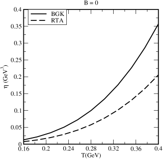
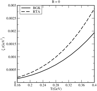
(a)	(b)

Figure 1: Shear viscosity (a) and bulk viscosity (b) as a function of $T$ in the absence of strong magnetic field

Having understood the relation between the transport coefficients: $\eta$ and $\zeta$ and the input in the transport equation: BGK and RT collision terms, we wish to see how a external strong magnetic field could affect the aforesaid relation in the next subsection.

3.2 Shear $(\eta_{B})$ and bulk $(\zeta_{B})$ viscosities in the presence of strong magnetic field

In this section, we will evaluate $\eta$ and $\zeta$ viscous coefficients of the magnetized hot QCD medium. The presence of magnetic field leads to the quantization of the quark energy in terms of the Landau levels as [102]

$$\omega_{i}=\sqrt{p_{3}^{2}+m_{i}^{2}+2n|q_{i}B|},$$ (75)

where $n=0,1,2....$ corresponds to various Landau levels. In addition to this, the phase space integral also gets modified as [102]

$$\int\frac{d^{3}p}{(2\pi)^{3}}\rightarrow\sum_{n=0}^{\infty}\frac{|q_{i}B|}{2\pi}\int\frac{dp_{3}}{2\pi}(2-\delta_{n0}).$$ (76)

In the SMF limit ($|q_{i}B|>>T^{2}$), there is a huge energy gap between the LLL and the higher landau levels (HLLs), hence, only $n=0$ state is populated. In this situation, motion of the quarks gets restricted in the transverse direction and becomes purely longitudinal (along the direction of the magnetic field i.e. $\mathbf{B}=B\hat{z}$). The quark contribution to the energy-momentum tensor will get modified (the gluon part remains as it is because gluons are not affected by the magnetic field directly). The quark part in LLL takes the form

$${T}_{B,q}^{\mu\nu}=2\sum_{i}\frac{g_{i}|q_{i}B|}{4\pi^{2}}\int dp_{3}~{}\frac{p^{\mu}p^{\nu}}{\omega_{i}}~{}f_{i}^{B},$$ (77)

where $f_{i}^{B}=f_{\rm eq,i}^{B}+\delta f_{i}^{B}$. $f_{\rm eq,i}^{B}$ is the equilibrium distribution function

$$f_{\mathrm{e}q,i}^{B}=\frac{1}{e^{\beta\omega_{i}}+1},$$ (78)

and $\omega_{i}=\sqrt{p_{3}^{2}+m_{i}^{2}}$. Now, we assume that the system has slightly deviated from the equilibrium, the dissipative part of the energy-momentum tensor reads as

$$\pi_{B,q}^{\mu\nu}=\sum_{i}\frac{g_{i}|q_{i}B|}{2\pi^{2}}\int dp_{3}~{}\frac{p^{\mu}p^{\nu}}{\omega_{i}}~{}\delta f_{i}^{B},$$ (79)

where $\delta f_{i}^{B}$ is the deviation in the distribution function of the quarks. In the effective (1+1) dimensional kinetic theory in the SMF, the RBTE for quarks takes the form

$$p^{\mu}\partial_{\mu}f^{B}_{i}(x,p) = -p^{\mu}u_{\mu}\nu_{i}^{B}\left(f^{B}_{i}-n^{B}_{i}n{{}^{B}}_{\mathrm{e}q,i}^{-1}f^{B}_{\mathrm{e}q,i}\right).$$ (80)

Here $p^{\mu}\equiv(p^{0},0,0,p^{3})$, $x^{\mu}\equiv(x^{0},0,0,x^{3})$ and $n_{\mathrm{e}q,i}^{B}$ refers to the equilibrium number density of the quarks which reads

$$n_{\mathrm{e}q,i}^{B} = \frac{g_{i}|q_{i}B|}{4\pi^{2}}\int dp_{3}~{}f_{\rm eq,i}^{B},$$ (81)

and $\nu_{i}^{B}$ is collision frequency which is given by the inverse of the relaxation time. In the strong $B$, $\tau_{i}^{B}$ depends on the longitudinal component of the momentum $p_{3}$ unlike in pure thermal medium (42) where $\tau_{i}$ remains constant and does not depend on momentum. The relaxation time has been computed in the presence of strong $B$ [8]

$$\tau_{i}^{B}(p_{3};T,|q_{i}B|)=\frac{\omega_{i}(e^{\beta\omega_{i}}-1)}{\alpha_{s}C_{F}m_{i}^{2}(e^{\beta\omega_{i}}+1)}{\left(\int\frac{dp^{\prime}_{3}}{\omega^{\prime}_{i}(e^{\beta\omega^{\prime}_{i}}+1)}\right)}^{-1},$$ (82)

where $C_{F}$ (=4/3) is the Casimir factor and $\alpha_{s}$ is the QCD coupling in the strong magnetic field (8).

We can solve the RBTE (80) upto first order to get the $\delta f^{B}_{i}$ as .

$$\delta f^{B}_{i} = \delta f{{}^{B}}_{i}^{(0)}+g_{i}n_{\mathrm{e}q,i}^{-1}f_{\mathrm{e}q,i}\int_{p_{3}^{\prime}}\delta f{{}^{B}}_{i}^{(0)},$$ (83)

where

$$\delta f{{}^{B}}_{i}^{(0)} = -\frac{\tau_{i}^{B}}{p^{\nu}u_{\nu}}~{}p^{\mu}\partial_{\mu}f^{B}_{i}(x,p)$$ (84)

$$= -\frac{\tau_{i}^{B}}{\omega_{i}T}~{}p^{\mu}f^{B}_{\mathrm{e}q,i}(1-f^{B}_{\mathrm{e}q,i})\left[u_{\alpha}p^{\alpha}u_{\mu}\frac{DT}{T}+u_{\alpha}p^{\alpha}\frac{\nabla_{\mu}T}{T}-u_{\mu}p^{\alpha}Du_{\alpha}-p^{\alpha}\nabla_{\mu}u_{\alpha}\right].$$

Substituting $\delta f^{B}_{i}$ in (79), we finally obtain the spatial component of stress-energy tensor in the strong $\vec{B}$ as

$$\pi_{B,q}^{ij} = \sum_{i}\frac{g_{i}|q_{i}B|}{2\pi^{2}}\int dp_{3}~{}\frac{p^{i}p^{j}}{\omega_{i}T}\bigg{\{}\tau^{B}_{i}f{{}^{B}}_{\mathrm{e}q,i}(1-f^{B}_{\mathrm{e}q,i})\left[\bigg{(}\omega_{i}\left(\frac{\partial P}{\partial\varepsilon}\right)-\frac{p_{3}^{2}}{3\omega_{i}}\bigg{)}\partial_{l}u^{l}+p^{k}\left(\frac{\nabla_{k}P}{\varepsilon+P}-\frac{\nabla_{k}T}{T}\right)\right.$$ (85)

$$\left.-\frac{p^{k}p^{l}}{2\omega_{i}}W_{kl}\right]+g_{i}n{{}^{B}}_{\mathrm{e}q,i}^{-1}f{{}^{B}}_{\mathrm{e}q,i}\int_{p_{3}^{\prime}}\tau^{B}_{i}f{{}^{B}}_{\mathrm{e}q,i}(1-f{{}^{B}}_{\mathrm{e}q,i})\left[\bigg{(}\omega^{\prime}_{i}\left(\frac{\partial P}{\partial\varepsilon}\right)-\frac{p_{3}^{{}^{\prime}2}}{3\omega^{\prime}_{i}}\bigg{)}\partial_{l}u^{l}\right.$$

$$\left.+p^{\prime k}\left(\frac{\nabla_{k}P}{\varepsilon+P}-\frac{\nabla_{k}T}{T}\right)\right.\left.-\frac{p^{\prime k}p^{\prime l}}{2\omega^{\prime}_{i}}W_{kl}\right]\bigg{\}}.$$

Let us now understand the generic form of the tensorial structure of $\pi_{ij}$ in an external $\vec{B}$. The number of independent tensorial combinations (coefficients of viscosity) gets increased from two (in the absence of $\vec{B}$) to eight in the presence of $\vec{B}$. However, the number becomes seven due to the Onsager relation, out of which, five are the coefficients of shear-term, one is bulk-term and the last one is due to cross term between the ordinary and volume viscosities. In a medium (QGP), the cross term vanishes, moreover, in the presence of strong $\vec{B}$, the non-diagonal terms will also be absent due to the vanishing of transverse components of the velocity (artifact of strong $\vec{B}$). Thus, the tensorial structure gets reduced in a much simpler form, leaving the longitudinal components of the tensor survived, as

$$\pi_{xx}=-\eta_{0}\left(V_{zz}-\frac{1}{3}\nabla\cdot\mathbf{V}\right)+\zeta_{0}\nabla\cdot\mathbf{V},$$ (86)

$$\pi_{yy}=-\eta_{0}\left(V_{zz}-\frac{1}{3}\nabla\cdot\mathbf{V}\right)+\zeta_{0}\nabla\cdot\mathbf{V},$$ (87)

$$\pi_{zz}=2\eta_{0}\left(V_{zz}-\frac{1}{3}\nabla\cdot\mathbf{V}\right)+\zeta_{0}\nabla\cdot\mathbf{V},$$ (88)

where $\eta_{0}$ and $\zeta_{0}$ are known as the longitudinal viscosities and the other symbols are given in [12].

Similar to the case in the absence of magnetic field (53), the above components are grouped into the traceless and nonzero trace parts as

$$\pi_{xx}=\pi_{yy}=-\frac{1}{2}\pi_{zz}=-\eta_{0}\left(V_{zz}-\frac{1}{3}{\nabla\cdot\mathbf{V}|}_{z}\right),$$ (89)

$$\pi_{xx}=\pi_{yy}=\pi_{zz}=\zeta_{0}{\nabla\cdot\mathbf{V}|}_{z},$$ (90)

respectively. Therefore, the spatial component of the viscous tensor in strong $\vec{B}$ can be expressed in a form (by relabeling $\eta_{0}\equiv\eta_{B}$ and $\zeta_{0}\equiv\zeta_{B}$)

$$\pi_{B,q}^{ij}=-\eta_{B}W_{ij}-\zeta_{B}\delta_{ij}\partial_{l}u^{l}.$$ (91)

Now we can extract the coefficients $\eta_{B}$ and $\zeta_{B}$ from the coefficients of $W_{ij}$ and $\partial_{l}u^{l}$ in $\pi^{ij}$ obtained from kinetic theory (85). Since gluons are not directly affected by the strong magnetic field, we will take the gluon contribution (56) from Section 3.1 (in the absence of the magnetic field). Finally, the shear viscosity in the BGK collision term is expressed in terms of RT contribution as

$$\eta_{B}=\eta_{B}^{\rm RT}+\eta_{B}^{\rm corr},$$ (92)

where

$$\eta_{B}^{\rm RT} = \frac{\beta}{4\pi^{2}}\sum_{i}g_{i}|q_{i}B|\int dp_{3}~{}\frac{p_{3}^{4}}{\omega_{i}^{2}}\tau^{B}_{i}f{{}^{B}}_{\mathrm{e}q,i}(1-f^{B}_{\mathrm{e}q,i})+\frac{\beta}{15}g_{g}\tau_{g}\int\frac{d^{3}p}{(2\pi)^{3}}\frac{p^{4}}{\omega_{g}^{2}}~{}f_{\mathrm{e}q,g}(1+f_{\mathrm{e}q,g})$$ (93)

$$\eta_{B}^{\rm corr} = \frac{\beta}{4\pi^{2}}\sum_{i}g_{i}^{2}|q_{i}B|n{{}^{B}}_{\mathrm{e}q,i}^{-1}\int dp_{3}~{}\frac{p_{3}^{2}}{\omega_{i}(p_{3})}f{{}^{B}}_{\mathrm{e}q,i}(p_{3})\int_{p_{3}^{\prime}}\frac{{p^{\prime}_{3}}^{2}}{\omega_{i}(p^{\prime}_{3})}\tau^{B}_{i}(p^{\prime}_{3})f{{}^{B}}_{\mathrm{e}q,i}(p^{\prime}_{3})(1-f{{}^{B}}_{\mathrm{e}q,i}(p^{\prime}_{3}))$$ (94)

$$+\frac{\beta}{15}g_{g}^{2}~{}n_{\mathrm{e}q,g}^{-1}~{}\tau_{g}\int\frac{d^{3}p}{(2\pi)^{3}}\frac{p^{2}}{\omega_{g}(p)}~{}f_{\mathrm{e}q,g}(p)\int_{p^{\prime}}\frac{p^{\prime 2}}{\omega_{g}(p^{\prime})}f_{\mathrm{e}q,g}(p^{\prime})(1+f_{\mathrm{e}q,g}(p^{\prime})).$$

We will now depict how the strong $B$ could modulate the correspondence between the collision integrals and the (momentum) transport coefficients in Fig. 2. For a thermal medium in a strong $B$ environment, the dominant scale will now be the magnetic field ($|q_{f}B|>T^{2}$), unlike the temperature is the dominant scale in a thermal medium in the absence of magnetic field ($B=0$).

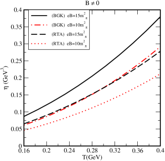
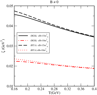
(a)	(b)

Figure 2: Shear viscosity (a) and bulk viscosity (b) as a function of $T$ in the presence of strong $B$.

We observe that similar to $B=0$ case, the shear viscosity in a strong $B$ with BGK collision term is still larger ($\sim$ 1.3 times) than the simple minded RT term, which is again evidenced by the fact that the correction term $\eta_{B}^{\rm corr}$ is always positive. In addition, in the presence of strong $B$, $\eta$ in both collision terms gets enhanced. To be precise, the enhancement with RT term is relatively larger than the BGK term. In strong $B$, the shear viscosity gets enhanced in BGK collision integral in comparison to RTA at a fixed $B$. $\eta$ also increases with the strength of the magnetic field in BGK as well as RTA collision terms.

One important observation we notice in Figure 2 (a) is that $\eta$ with BGK collision term at lower (strong) $B$, say $eB=10m_{\pi}^{2}$ looks similar to $\eta$ with RT term at higher (strong) $B$, say $eB=15m_{\pi}^{2}$. This leads to an ambiguity in the phenomenological modeling while extracting the physical parameters of the system by comparing the results from theory to the experiments. It means that if one were to extract the physical parameters from a comparison of theory to experiment one would deduce different values for the strength of B whether on uses BGK or RTA. In this case, it would be better to take results from BGK collision integral to compute the physical parameters since it shows an improvement over the naive RTA in the sense that it conserve the particle number and charge instantaneously.

Similarly, the bulk viscosity can be decomposed as

$$\zeta_{B}=\zeta^{\rm RT}_{B}+\zeta^{\rm corr}_{B},$$ (95)

where

$$\zeta_{B}^{\rm RT} = \frac{1}{2\pi^{2}}\sum_{i}g_{i}|q_{i}B|\int dp_{3}~{}\frac{p_{3}^{2}}{\omega_{i}}~{}f{{}^{B}}_{\mathrm{e}q,i}(1-f^{B}_{\mathrm{e}q,i})~{}A^{B}_{i,1}$$ (96)

$$+\frac{1}{3}g_{g}\int\frac{d^{3}p}{(2\pi)^{3}}\frac{p^{2}}{\omega_{g}}~{}f_{\mathrm{e}q,g}(1+f_{\mathrm{e}q,g})~{}A_{g,1},$$

$$\zeta_{B}^{\rm corr} = \frac{1}{2\pi^{2}}\sum_{i}g^{2}_{i}|q_{i}B|n{{}^{B}}_{\mathrm{e}q,i}^{-1}\int dp_{3}~{}\frac{p_{3}^{2}}{\omega_{i}}f{{}^{B}}_{\mathrm{e}q,i}(p_{3})\int_{p_{3}^{\prime}}f{{}^{B}}_{\mathrm{e}q,i}(p^{\prime}_{3})(1-f{{}^{B}}_{\mathrm{e}q,i}(p^{\prime}_{3}))~{}A^{B}_{i,2}$$ (97)

$$+\frac{1}{3}g_{g}^{2}~{}n_{\mathrm{e}q,g}^{-1}~{}\int\frac{d^{3}p}{(2\pi)^{3}}\frac{p^{2}}{\omega_{g}}f_{\mathrm{e}q,g}(p)\int_{p^{\prime}}f_{\mathrm{e}q,g}(p^{\prime})(1+f_{\mathrm{e}q,g}(p^{\prime}))~{}A_{g,2},$$

where the factors $A^{B}_{i,1}$ and $A^{B}_{i,2}$ are

$$A^{B}_{i,1} = \frac{\tau^{B}_{i}}{3T}\bigg{\{}\frac{p_{3}^{2}}{\omega_{i}}-3~{}\omega_{i}\left(\frac{\partial P}{\partial\varepsilon}\right)\bigg{\}},$$ (98)

$$A^{B}_{i,2} = \frac{\tau^{B}_{i}}{3T}\bigg{\{}\frac{p^{\prime}_{3}{{}^{2}}}{\omega_{i}}-3~{}\omega_{i}\left(\frac{\partial P}{\partial\varepsilon}\right)\bigg{\}}.$$ (99)

Applying the Landau-Lifshitz condition (i.e. $\pi_{B,q}^{00}=0$) and following the similar steps as the $B=0$ case, we get the final expression for the bulk viscosity of the strongly magnetized thermal QCD medium (95) as

$$\zeta_{B}^{\rm RT} = \frac{\beta}{6\pi^{2}}\sum_{i}g_{i}|q_{i}B|\int dp_{3}~{}\tau^{B}_{i}~{}f{{}^{B}}_{\mathrm{e}q,i}(1-f^{B}_{\mathrm{e}q,i})~{}\bigg{\{}\frac{p_{3}^{2}}{\omega_{i}}-3\omega_{i}\left(\frac{\partial P}{\partial\varepsilon}\right)\bigg{\}}^{2}$$ (100)

$$+\frac{\beta}{9}g_{g}\tau_{g}\int\frac{d^{3}p}{(2\pi)^{3}}~{}f_{\mathrm{e}q,g}(1+f_{\mathrm{e}q,g})\bigg{\{}\frac{p^{2}}{\omega_{g}}-3\omega_{g}\left(\frac{\partial P}{\partial\varepsilon}\right)\bigg{\}}^{2},$$

$$\zeta_{B}^{\rm corr} = \frac{\beta}{6\pi^{2}}\sum_{i}g^{2}_{i}|q_{i}B|n{{}^{B}}_{\mathrm{e}q,i}^{-1}\int dp_{3}~{}\frac{p_{3}^{2}}{\omega_{i}}f{{}^{B}}_{\mathrm{e}q,i}(p_{3})\int_{p_{3}^{\prime}}\tau^{B}_{i}(p^{\prime}_{3})f{{}^{B}}_{\mathrm{e}q,i}(p^{\prime}_{3})(1-f{{}^{B}}_{\mathrm{e}q,i}(p^{\prime}_{3}))$$ (101)

$$\times\bigg{\{}\frac{p^{\prime}_{3}{{}^{2}}}{\omega^{\prime}_{i}}-3\omega^{\prime}_{i}\left(\frac{\partial P}{\partial\varepsilon}\right)-b^{\prime}_{i}\omega_{i}^{\prime}\bigg{\}}+\frac{\beta}{9}g_{g}^{2}~{}n_{\mathrm{e}q,g}^{-1}\tau_{g}~{}\int\frac{d^{3}p}{(2\pi)^{3}}\frac{p^{2}}{\omega_{g}}f_{\mathrm{e}q,g}(p)\int_{p^{\prime}}f_{\mathrm{e}q,g}(p^{\prime})$$

$$\times(1+f_{\mathrm{e}q,g}(p^{\prime}))\bigg{\{}\frac{p^{\prime 2}}{\omega^{\prime}_{g}}-3\omega^{\prime}_{g}\left(\frac{\partial P}{\partial\varepsilon}\right)-b^{\prime}_{g}\omega^{\prime}_{g}\bigg{\}},$$

where

$$b^{\prime}_{i}=\frac{\sum_{i}g^{2}_{i}|q_{i}B|n{{}^{B}}_{\mathrm{e}q,i}^{-1}\int dp_{3}~{}\omega_{i}f{{}^{B}}_{\mathrm{e}q,i}(p_{3})\int_{p_{3}^{\prime}}f{{}^{B}}_{\mathrm{e}q,i}(p^{\prime}_{3})(1-f{{}^{B}}_{\mathrm{e}q,i}(p^{\prime}_{3}))~{}\bigg{\{}\frac{p^{\prime}_{3}{{}^{2}}}{\omega^{\prime}_{i}}-3\omega^{\prime}_{i}\left(\frac{\partial P}{\partial\varepsilon}\right)\bigg{\}}}{\sum_{i}g^{2}_{i}|q_{i}B|n{{}^{B}}_{\mathrm{e}q,i}^{-1}\int dp_{3}~{}\omega_{i}f{{}^{B}}_{\mathrm{e}q,i}(p_{3})\int_{p_{3}^{\prime}}f{{}^{B}}_{\mathrm{e}q,i}(p^{\prime}_{3})(1-f{{}^{B}}_{\mathrm{e}q,i}(p^{\prime}_{3}))\omega^{\prime}_{i}}.$$ (102)

We have also now plotted bulk viscosity ($\zeta$) as a function of temperature in the presence of strong magnetic field in the above Fig. 2 (right panel). It is found that RT collision term is still found to dominate over BGK term except at higher temperature, where their contributions are almost same. This observation is just opposite to the observation in the absence of magnetic field (seen in Fig. 1), where the merger happens to be in the small temperature region.

3.3 Charge and heat transport coefficients in thermal QCD medium

In this subsection, we will revisit our earlier work [43] wherein we have calculated the electrical ($\sigma_{el}$) and thermal ($\kappa$) conductivities of the hot QCD medium in both BGK and RT collision integrals. We will use $\sigma_{el}$ and $\kappa$ to study the relative competition between the various transport coefficients in section 4.

3.3.1 Electrical conductivity

The electrical conductivity $\sigma_{el}$, which manifests the ease of electric current flow in the medium has been calculated in the kinetic theory framework using the BGK type collision integral. It can be decomposed into two parts in a similar fashion like $\eta$ and $\zeta$ in the absence of the magnetic field as

$$\sigma_{el}=\sigma_{el}^{\rm RT}+\sigma_{el}^{\rm corr},$$ (103)

where

$$\sigma_{\rm el}^{\rm RT} = \frac{2\beta}{3\pi^{2}}\sum_{i}q_{i}^{2}g_{i}\tau_{i}\int dp~{}\frac{p^{4}}{\omega_{i}^{2}}f_{\mathrm{e}q,i}(p)(1-f_{\mathrm{e}q,i}(p)),$$ (104)

$$\sigma_{\rm el}^{\rm Corr} = \frac{2\beta}{\pi^{2}}\sum_{i}q_{i}^{2}g^{2}_{i}\tau_{i}n_{\mathrm{e}q,i}^{-1}\int dp~{}\frac{p^{3}}{\omega_{i}}f_{\mathrm{e}q,i}(p)\int_{p^{\prime}}\frac{p^{\prime}}{\omega^{\prime}_{i}}f_{\mathrm{e}q,i}(p^{\prime})(1-f_{\mathrm{e}q,i}(p^{\prime})),$$ (105)

and in the strong magnetic field

$$\sigma_{el}^{B}=\sigma_{el}^{\rm B,RT}+\sigma_{el}^{\rm B,corr},$$ (106)

where

$$\sigma^{B,\rm RT}_{el} = \frac{\beta}{\pi^{2}}\sum_{i}q_{i}^{2}g_{i}|q_{i}B|\int{dp_{3}}\frac{p_{3}^{2}}{\omega_{i}^{2}}\tau_{i}^{B}f_{\mathrm{e}q,i}^{B}(1-f_{\mathrm{e}q,i}^{B}),$$ (107)

$$\sigma^{B,\rm Corr}_{el} = \frac{\beta}{\pi^{2}}\sum_{i}q_{i}^{2}g^{2}_{i}|q_{i}B|{n_{\mathrm{e}q,i}^{B}}^{-1}\left[\int{dp_{3}}\frac{p_{3}}{\omega_{i}}f_{\rm eq,i}^{B}(p_{3})\int_{p^{\prime}_{3}}\frac{p^{\prime}_{3}}{\omega^{\prime}_{i}}~{}\tau_{i}^{B}(p_{3}^{\prime})~{}f_{\rm eq,i}^{B}(p^{\prime}_{3})~{}(1-f_{\rm eq,i}^{B}(p^{\prime}_{3}))\right].$$

3.3.2 Thermal conductivity

We have also calculated the heat transport coefficient namely thermal conductivity ($\kappa$) from the difference between the energy diffusion and the enthalpy diffusion using the BGK collision integral. It can be written in the absence of the magnetic field as

$$\kappa=\kappa^{\rm RT}+\kappa^{\rm Corr},$$ (109)

where

$$\kappa^{\rm RT} = \frac{\beta^{2}}{3\pi^{2}}\sum_{i}g_{i}\tau_{i}\int dp\frac{p^{4}}{\omega_{i}^{2}(p)}(\omega_{i}(p)-h_{i})^{2}f_{\rm eq,i}(p)(1-f_{\rm eq,i}(p)),$$ (110)

$$\kappa^{\rm Corr} = \frac{\beta^{2}}{\pi^{2}}\sum_{i}g^{2}_{i}\tau_{i}n_{\mathrm{e}q,i}^{-1}\int dp\frac{p^{3}}{\omega_{i}(p)}(\omega_{i}(p)-h_{i})f_{\rm eq,i}(p)$$ (111)

$$\times\int_{p^{\prime}}\frac{p^{\prime}}{\omega_{i}(p^{\prime})}(\omega_{i}(p^{\prime})-h_{i})f_{\rm eq,i}(p^{\prime})(1-f_{\rm eq,i}(p^{\prime})),$$

and in the strong magnetic field as

$$\kappa^{B}=\kappa^{\rm B,RT}+\kappa^{\rm B,Corr},$$ (112)

where

$$\kappa^{\rm B,RT} = \frac{\beta^{2}}{2\pi^{2}}\sum_{i}{g_{i}|q_{i}B|}\int{dp_{3}}\frac{p_{3}^{2}}{\omega_{i}^{2}}\tau_{i}^{B}(\omega_{i}-h_{i}^{B})^{2}f_{\rm eq,i}^{B}(1-f_{\rm eq,i}^{B}),,$$ (113)

$$\kappa^{\rm B,Corr} = \frac{\beta^{2}}{2\pi^{2}}\sum_{i}{g^{2}_{i}|q_{i}B|}{n_{\mathrm{e}q,i}^{B}}^{-1}\int{dp_{3}}\frac{p_{3}}{\omega_{i}}(\omega_{i}-h_{i}^{B})f_{\rm eq,i}^{B}(p_{3})$$ (114)

$$\times\int_{p^{\prime}_{3}}\frac{p^{\prime}_{3}}{\omega^{\prime}_{i}}\tau_{i}^{B}(p^{\prime}_{3})(\omega^{\prime}_{i}-h_{i}^{B})f_{\rm eq,i}^{B}(p^{\prime}_{3})(1-f_{\rm eq,i}^{B}(p^{\prime}_{3})).$$

4 Applications

In this section, we will study how BGK collision integral modifies the specific shear and bulk viscosities needed to explore the fluidity and transition point of the QCD phase. We will further check the relative behavior among the momentum, heat, and charge diffusion in the strongly magnetized QCD medium. These derived coefficients namely Prandtl number, Reynolds number and $\gamma$ factor characterize the various properties like degree of sound attenuation in the medium, nature of the flow, etc. At last, we see the relative competition between the shear and bulk viscosities in terms of ratio $\zeta/\eta$.

4.1 Specific shear ($\eta/s$) and bulk ($\zeta/s$) viscosities

We will now focus on the ratios $\eta/s$ and $\zeta/s$, also known as specific shear and specific bulk viscosities, respectively. These ratios give an idea about the perfectness and conformal nature of the fluid, respectively. The ratio $\eta/s$ has been calculated for the QGP using the parton transport method [103] and was found to be very small, confirming the strongly coupled nature of the QGP, which nullifies the widespread belief that QGP happens to be a weakly interacting gas of quarks and gluons. This is also in agreement with the famous KSS bound of the AdS/CFT correspondence [44]. The relativistic viscous hydrodynamics  [46] also uses very small value of $\eta/s$ ratio (around 0.08 to 0.1) to reproduce the RHIC data [50] and also matches well with lattice calculations [51]. The entropy density of the hot QCD medium can be defined using the thermodynamical relation

$$s=\frac{(\varepsilon+P)}{T},$$ (115)

where $\varepsilon$ and $P$ are the energy density and pressure, respectively. First, we calculate $\varepsilon$ and $P$ for $B=0$ case as

$$\varepsilon = \frac{1}{\pi^{2}}\sum_{i}g_{i}\int dp~{}p^{2}\omega_{i}~{}f_{\mathrm{e}q,i}+\frac{g_{g}}{2\pi^{2}}\int dp~{}p^{2}~{}\omega_{g}~{}f_{\mathrm{e}q,g},$$ (116)

$$P = \frac{1}{{3\pi^{2}}}\sum_{i}g_{i}\int dp~{}\frac{p^{4}}{\omega_{i}}~{}f_{\mathrm{e}q,i}+\frac{g_{g}}{6\pi^{2}}\int dp~{}\frac{p^{4}}{\omega_{g}}~{}f_{\mathrm{e}q,g},$$ (117)

respectively. In the strong magnetic field, we have

$$\varepsilon_{B} = \frac{1}{2\pi^{2}}\sum_{i}g_{i}|q_{i}B|\int dp_{3}~{}\omega_{i}~{}f_{\rm eq,i}^{B}+\frac{g_{g}}{2\pi^{2}}\int dp~{}p^{2}~{}\omega_{g}~{}f_{\mathrm{e}q,g},$$ (118)

$$P_{B} = \frac{1}{2\pi^{2}}\sum_{i}g_{i}|q_{i}B|\int dp_{3}~{}\frac{p_{3}^{2}}{\omega_{i}}~{}f_{\rm eq,i}^{B}+\frac{g_{g}}{6\pi^{2}}\int dp~{}\frac{p^{4}}{\omega_{g}}~{}f_{\mathrm{e}q,g}.$$ (119)

The entropy density in $B=0$ and $B\neq 0$ cases can be calculated from Eqn. (115) as

$$s = \frac{\beta}{3\pi^{2}}\sum_{i}g_{i}\int dp~{}p^{2}\left(\frac{p^{2}}{\omega_{i}}+3\omega_{i}\right)f_{\mathrm{e}q,i}+\frac{\beta}{6\pi^{2}}g_{g}\int dp~{}p^{2}\left(\frac{p^{2}}{\omega_{g}}+3\omega_{i}\right)f_{\mathrm{e}q,g},$$ (120)

$$s_{B} = \frac{\beta}{2\pi^{2}}\sum_{i}g_{i}|q_{i}B|\int dp_{3}~{}\left(\frac{p_{3}^{2}}{\omega_{i}}+\omega_{i}\right)f_{\rm eq,i}^{B}+\frac{\beta}{6\pi^{2}}g_{g}\int dp~{}p^{2}\left(\frac{p^{2}}{\omega_{g}}+3\omega_{i}\right)f_{\mathrm{e}q,g},$$ (121)

respectively.

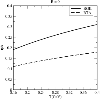
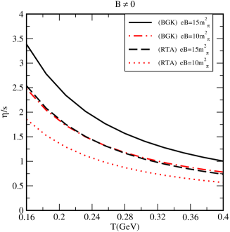
(a)	(b)

Figure 3: Shear viscosity to entropy density ratio $(\eta/s)$ as a function of $T$ in absence (a) and in presence (b) of the strong $B$

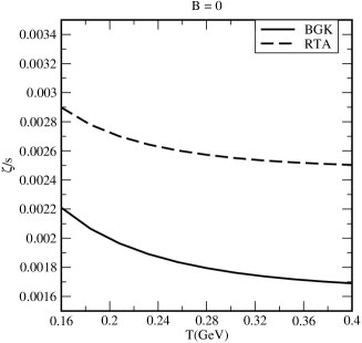
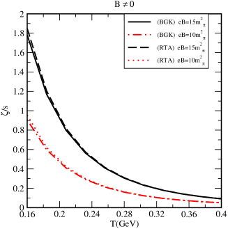
(a)	(b)

Figure 4: Bulk viscosity to entropy density ratio $(\zeta/s)$ as a function of $T$ in absence (a) and in presence (b) of the strong $B$

Fig. 3 shows our estimates of the ratio $\eta/s$ as a function of temperature in the absence (left panel) and presence of the strong $B$ (right panel). The ratio $\eta/s$ increases (decreases) with $T$ in the absence (presence) of the strong $B$. The magnitude of $\eta/s$ gets enhanced in the BGK collision integral in both cases. It indicates that instantaneous conservation of the particle number in the medium takes the fluid away from its ideal nature. The $\eta/s$ ratio gets enhanced in strong $B$. Like the case of $\eta$ in a strong $B$ in Fig. 2 (a), $\eta/s$ ratio in BGK collision term at $eB=10m_{\pi}^{2}$ also looks similar to its counterpart with RT term at $eB=15m_{\pi}^{2}$. As we mentioned earlier, this similarity leads to an apparent ambiguity in extracting the physical parameters by comparing the theoretical predictions to the experimental data. It would be better to prefer BGK collision term over RTA.

In Fig. 4, we have displayed the ratio $\zeta/s$ as a function of temperature. We found that $\zeta/s$ decreases with $T$ in $B=0$ (left panel) as well as in $B\neq 0$ (right panel) case. The magnitude of $\zeta/s$ gets reduced in the BGK collision term in comparison to the RT in the $B=0$ scenario while there in the presence of strong $B$, both the collision integrals produce similar results. It further increases as the strength of $B$ grows, which may indicate that the system moves away from the conformal nature due to the presence of the strong magnetic field.

4.2 Prandtl number

The ratio of the momentum diffusivity to the thermal diffusivity in a given medium is quantified in terms of the Prandtl number (Pr)

$${\rm Pr}=\frac{\eta/\rho}{\kappa/C_{p}},$$ (122)

where $\rho$ is the mass density, $C_{P}$ denotes the specific heat at constant pressure and $\kappa$ refers to the thermal conductivity of the medium under consideration. Pr gives an idea about the roles of the shear viscosity and thermal conductivity on the sound attenuation in a system. The smaller value of the Pr number (Pr $<<1$) corresponds to the dominance of the thermal diffusion while higher value (Pr $>>1$) to that of momentum diffusion. The specific heat $C_{P}$ can be calculated from the thermodynamic relation

$$C_{p}=\frac{\partial}{\partial T}(\varepsilon+P),$$ (123)

where $\varepsilon$ and $P$ are the energy density and pressure, respectively and have been calculated in the absence [Eqns. (116) and (117)] as well as in the presence of strong $B$ [Eqns. (118) and (119)]. The specific heat $C_{P}$ can be evaluated in the absence and in presence of the SMF as

$$C_{p} = \frac{\beta^{2}}{3\pi^{2}}\sum g_{i}\int dp~{}p^{2}(p^{2}+3\omega_{i}^{2})~{}f_{\rm eq,i}(1-f_{\rm eq,i})$$ (124)

$$+\frac{\beta^{2}}{6\pi^{2}}g_{g}\int dp~{}p^{2}(p^{2}+3\omega_{g}^{2})~{}f_{\mathrm{e}q,g}(1+f_{\mathrm{e}q,g}),$$

and

$$C^{B}_{p} = \frac{\beta^{2}}{2\pi^{2}}\sum_{i}g_{i}|q_{i}B|\int dp_{3}~{}(p_{3}^{2}+\omega_{i}^{2})~{}f_{\rm eq,i}^{B}(1-f_{\mathrm{e}q,i}^{B})$$ (125)

$$+\frac{\beta^{2}}{6\pi^{2}}g_{g}\int dp~{}p^{2}(p^{2}+3\omega_{g}^{2})~{}f_{\mathrm{e}q,g}(1+f_{\mathrm{e}q,g}),$$

respectively. Another quantity that we need to study the Pr number is the mass density $(\rho)$. In our case, the mass density is defined as

$$\rho=2\sum_{i}m_{i}n_{i}+m_{g}n_{g},$$ (126)

where $m_{i}~{}(m_{g})$ are the quasi-particle masses of the quarks (gluons), generated due to the presence of the thermal medium. Apart from it, $n_{eq,i}$ and $n_{eq,g}$ are the number densities of the quarks and gluons, respectively which can be calculated using the phase space distribution functions [Eqns. (39) and (41)]. The mass density in the absence of the magnetic field reads

$$\rho=\frac{1}{\pi^{2}}\sum_{i}m_{i}g_{i}\int dp~{}p^{2}f_{\rm eq,i}+\frac{1}{2\pi^{2}}m_{g}g_{g}\int dp~{}p^{2}f_{\mathrm{e}q,g},$$ (127)

and for a strongly magnetized medium, it is

$$\rho^{B}=\frac{1}{2\pi^{2}}\sum_{i}m_{i}g_{i}|q_{i}B|\int dp_{3}~{}f_{\rm eq,i}^{B}+\frac{1}{2\pi^{2}}m_{g}g_{g}\int dp~{}p^{2}f_{\mathrm{e}q,g}.$$ (128)

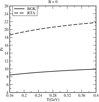
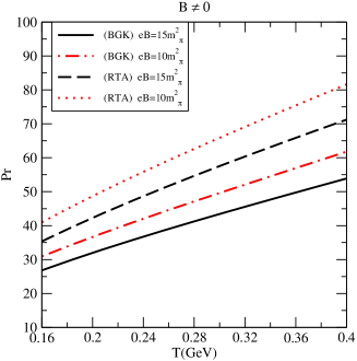
(a)	(b)

Figure 5: Prandtl number as a function of $T$ in the absence (a) and in the presence (b) of the strong $B$

Now we will focus on our results of the Prandtl number. In the left panel of fig. 5, we have shown the Pr number as a function of the temperature in the absence of $B$. It is found to be increasing monotonically with $T$ in both BGK and RT collision integrals. The magnitude is greater than one in both the collision terms which means that in a medium consisting of quarks and gluons, the rate of momentum diffusion dominates over that of thermal diffusion. The magnitude gets reduced in the BGK collision integral. The reduction in the Pr number may lead to the conclusion that instantaneous conservation of the particle number enforces less pronounced momentum transport. We carry out similar investigations in the presence of the strong $B$ in the right panel of fig. 5 and observe similar trends with the temperature. There is an enhancement in the magnitude of the Pr number, but its behavior with the collision integrals is similar i.e. RT collision integral dominates over the BGK. It decreases with the magnetic field. Pr number has been evaluated earlier for many systems such as dilute atomic Fermi gas [65] and has been reported to be around $\frac{2}{3}$ at high temperature. In case of non-relativistic conformal holographic fluid [64] it has been found to be around $1.0$ and for strongly coupled liquid helium, $2.5$. [63].

4.3 Reynolds number

From a hydrodynamic point of view, the Reynolds number has an essential significance in determining the nature of the flow pattern of a fluid. The small value of the Reynolds number indicates the laminar flow, while a large one tells about the turbulence. It is defined as

$${\rm RI}=\frac{Lv}{\eta/\rho},$$ (129)

where $L$ refers to the characteristic length while $v$ to the relative velocity of the fluid, respectively. The magnitude of the RI gives an idea about the kinematic viscosity $\eta/\rho$ of the fluid in comparison to the characteristic length and the relative speed. The large value (in case of turbulent flow) of the RI corresponds to the small magnitude of $\eta/\rho$ in comparison to the quantity $Lv$ of the system.

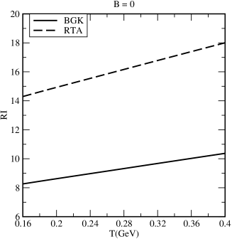
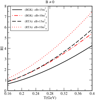
(a)	(b)

Figure 6: Reynolds number as function of $T$ in absence (a) and in presence (b) of the strong $B$

To study the impact of the BGK collision term on the nature of the flow of the thermal QCD medium, we plot Reynolds number in the left panel of Fig. 6 with $T$ in the absence of the magnetic field. RI increases with the temperature and its magnitude gets lowered in the BGK type collision integral in comparison to the RT, which indicates that instantaneous conservation of particle number promotes the laminar nature of the flow. The value of the RI is found to be around $8-10$ for BGK and $14-18$ for RT in the temperature range $160<T<400$ MeV. In a (3 + 1)-dimensional fluid dynamical model, the value of the RI is estimated in the range $3-10$ for initial QGP with $\eta/s=$ 0.1 [66], The holographic model reports its upper bound as 20 [67]. In the right panel, we perform similar studies in the presence of strong magnetic field. The trends are similar to the $B=0$ case i.e. it increases with $T$ and its magnitude gets reduced in BGK term. However, RI shows decreasing trends with increasing $B$. The value of the RI is roughly in the range of $1-8$ as $T$ is varied from $160$ to $400$ MeV for the two strengths of the magnetic field i.e. $eB=15m^{2}_{\pi}$ and $eB=10m^{2}_{\pi}$. We have observed that the RI is reduced in the presence of strong $B$ as compared to $B=0$ case and this reduction is more pronounced in the low $T$ region around the QCD transition point.

As seen earlier, the temperature dependence of $\eta$ and $\eta/s$ with BGK collision term at $eB=10m_{\pi}^{2}$ shows a similar behaviour with its counterpart with RT collision term at $eB=15m_{\pi}^{2}$ in Fig. 2 (a) and Fig. 3 (b), respectively. Apart from the size of the system ($L$) and the relative velocity ($v$), Reynolds number is obtained from the inverse of kinematic viscosity ($\eta/\rho$), so RI also shows a similarity between BGK predictions at $eB=10m_{\pi}^{2}$ and RT predictions at $eB=15m_{\pi}^{2}$. This similarity leads to an ambiguity in the phenomenological modeling. The BGK collision term should be prefered over RTA for the extraction of phenomenologically relavant quantities from experimental data.

4.4 Momentum diffusion vs charge diffusion

The relative competition between the momentum diffusion and charge diffusion can be better understood through a dimensionless ratio

$$\gamma=\frac{\eta/s}{\sigma_{el}/T},$$ (130)

where $\sigma_{el}$ is the electrical conductivity. The quarks, unlike gluons, are electrically charged particles, hence, contribute to $\sigma_{el}$, while both quarks and gluons contribute to the momentum transport, hence, contribute to the shear viscosity. The ratio $\gamma$ gives an idea about the relative significance of the matter and gluon sector contributions to the momentum and charge diffusion in the hot QCD medium.

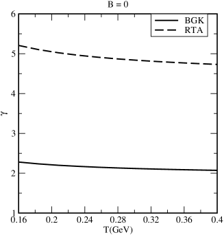
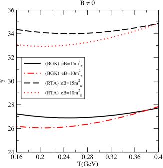
(a)	(b)

Figure 7: Dimensionless ratio $\gamma$ as a function of $T$ in absence (a) and in presence (b) of the strong $B$.

In Fig. 7, we have shown the dimensionless ratio $\gamma$ calculated in Eqn. (130) as a function of $T$ in the absence of $B$ (in the left panel) and have found that $\gamma$ decreases slowly with temperature near the crossover point ($\sim 160)$ MeV and then almost remains constant at higher temperatures. The magnitude of the $\gamma$ factor gets reduced in the BGK collision integral, which indicates that conservation of particle number enhances the charge transport in the medium at a greater rate in comparison to momentum transport. In the right panel of Fig. 7, we have displayed the ratio $\gamma$ with temperature in the presence of the strong $B$ and have observed the reduction of $\gamma$ in BGK collision term like the $B=0$ case. The $\gamma$ factor first decreases with $T$ and then increases. Its magnitude is higher when the strength of the magnetic field is $eB=15m^{2}_{\pi}$ in comparison to $eB=10m^{2}_{\pi}$.

4.5 Bulk viscosity vs shear viscosity

The relative competition between the shear viscous and bulk viscous nature of the fluid can be understood in terms of the ratio $\zeta/\eta$. This ratio has been calculated for a variety of systems in the different frameworks. In the case of interacting scalar field [70], $\zeta/\eta$ has been found to be around $15\left(\frac{1}{3}-c_{s}^{2}\right)^{2}$ (where $c_{s}$ refers to the speed of sound in the medium). For hot QCD medium using the perturbation theory, it is nearly equal to $15\left(\frac{1}{3}-c_{s}^{2}\right)^{2}$  [60], and for strongly coupled gauge plasma, $2\left(\frac{1}{3}-c_{s}^{2}\right)^{2}$ [104]. In holographic model [71], the ratio $\zeta/\eta$ is found to be less than $0.5$ at high temperatures and it is around $0.6$ in the phase transition region. In another attempt [72], the authors notice that $\zeta$ is smaller than $\eta$ at high temperatures but acquires higher values around critical temperature ($T_{c}$) of the phase transition. In the case of quasi-gluon plasma [73], the ratio $\zeta/\eta$ behaves like that found using the perturbative QCD at higher temperatures (above $1.5~{}T_{c}$) but for $T$ around $1.02~{}T_{c}$, nonperturbative effects become significant.

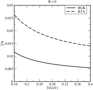
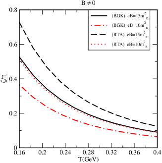
(a)	(b)

Figure 8: Bulk to shear viscosity $(\zeta/\eta)$ ratio as a function of $T$ in absence (a) and in presence (b) of the strong $B$

Now we will explore the ratio $\zeta/\eta$ for our case. In fig. 8, the variation of the ratio $\zeta/\eta$ with temperature has been shown. It decreases with $T$ and gets reduced in BGK collision term in the absence [Fig. 8 (a)] as well as in the presence of strong $B$ [Fig. 8 (b)]. In the absence of $B$, the magnitude of the ratio $\zeta/\eta$ remains less than one in the temperature range $160-400$ MeV that corresponds to the dominance of $\eta$ over $\zeta$. In SMF, the ratio $\zeta/\eta$ gets enhanced slightly, but the magnitude is still, less than one and the RT collision term dominates over BGK.

5 Conclusion

To conclude, we have examined the relative behavior of the transport coefficients of the thermal QCD medium in BGK and RT collision integrals. This study helps us in probing the various salient features of the collision integrals and their impact on the transport phenomenon. For that purpose, we have evaluated shear and bulk viscosities using the relativistic Boltzmann transport equation where collisional aspects of the medium have been incorporated with the help of BGK type collision integral, which exhibits an improvement over RT enforcing the conservation of particles in the medium. Then using $\eta$ and $\zeta$, we have studied the ratios $\eta/s$ and $\zeta/s$ to get an idea about the ideal and conformal nature of the fluid. We further explored the relative significance of the various transport coefficients through Prandtl number, Reynolds number, factor $\gamma$ and ratio $\zeta/\eta$. Both $\eta$ and $\zeta$ have been found to be increasing with the temperature in both the collision integrals but the magnitude of $\eta$ ($\zeta$) gets enhanced (reduced) in BGK collision term in comparison to RT. As a result, $\eta/s$ gets enhanced whereas $\zeta/s$ reduces. The magnitude of other derived coefficients Pr, RI, $\gamma$ and ratio $\zeta/\eta$ also gets reduced. Apart from it, the ratio $\eta/s$ ($\zeta/s$) is minimum (maximum) near $T_{c}$. Further, we studied the impact of strong $B$ on the collision integral and subsequently on the momentum transport in the medium where quark dynamics is restricted in only 1-D i.e. along the direction of the $B$. The abovementioned transport coefficients show similar trends with respect to the collision integral as $B=0$ case except for ratio $\zeta/s$, which is almost identical in both the collision integrals. The strong $B$ flips the $T$ dependence of $\zeta$ and $\eta/s$ which now shows decreasing trends. The ratio $\eta/s$ ($\zeta/s$) becomes smaller (larger). We also see enhancement of Pr, $\gamma$, and $\zeta/\eta$. Enhancement of Pr number leads to the conclusion that in a strong $B$, the sound attenuation is mostly controlled by $\eta$. In strong $B$, RI gets reduced, which indicates that strong B adds to the laminar nature of the flow. We see that different collision integral gives different values of the transport coefficients which are experimentally measurable quantities. Thus using this one-to-one correspondence, we can sense the collision integral responsible for the equilibration of the medium. In this study, the hot QCD medium effects have been incorporated via dispersion relations wherein the masses of the quasi-partons are parameterized according to a thermodynamically consistent quasi-particle model. We calculate the medium-generated thermal masses of the partons by taking the poles of the resummed propagators calculated under the framework of perturbative thermal QCD with a strong $B$ in the background.

Appendix A Derivation of the left hand side in equation (43)

The BGK collision term (right hand side) of  (36) is given as

$$C[f] = -p^{\mu}u_{\mu}\nu_{i}\left(f_{i}-n_{{}_{i}}n_{\mathrm{e}q,i}^{-1}f_{\mathrm{e}q,i}\right),$$ (A.131)

$$= -p^{\mu}u_{\mu}\nu_{i}\left(f_{i}-\frac{g_{i}\int_{p}(f_{\mathrm{e}q,i}+\delta f_{i})}{n_{\mathrm{e}q,i}}f_{\mathrm{e}q,i}\right),$$

$$= -p^{\mu}u_{\mu}\nu_{i}\left(f_{i}-\frac{(g_{i}\int_{p}f_{\mathrm{e}q,i}+g_{i}\int_{p}\delta f_{i})}{n_{\mathrm{e}q,i}}f_{\mathrm{e}q,i}\right),$$

$$= -p^{\mu}u_{\mu}\nu_{i}\left(\delta f_{i}-g_{i}n_{\mathrm{e}q,i}^{-1}f_{\mathrm{e}q,i}\int_{p}\delta f_{i}\right).$$

Appendix B Quark self energy in imaginary time formalism

We can approximate the exponential factor in (10) as $e^{-k_{\perp}/|q_{i}B|}\approx 1$, since the transverse component of the quark momentum is almost negligible i.e. $k_{\perp}\approx 0$. The quark self energy (7) takes the form

$$\Sigma(p_{\parallel}) = \frac{2g^{2}}{3\pi^{2}}|q_{i}B|T\sum_{n}\int dk_{z}\frac{\left[\left(1+\gamma^{0}\gamma^{3}\gamma^{5}\right)\left(\gamma^{0}k_{0}-\gamma^{3}k_{z}\right)-2m_{i}\right]}{\left[k_{0}^{2}-\omega^{2}_{k}\right]\left[(p_{0}-k_{0})^{2}-\omega_{pk}^{2}\right]}$$ (B.132)

$$= \frac{2g^{2}|q_{i}B|}{3\pi^{2}}\int dk_{z}\left[(\gamma^{0}+\gamma^{3}\gamma^{5})L^{1}-(\gamma^{3}+\gamma^{0}\gamma^{5})k_{z}L^{2}\right],$$

where $\omega_{k}^{2}=k_{z}^{2}+m_{i}^{2}$, $\omega_{pk}^{2}=(p_{z}-k_{z})^{2}$ and $L^{1}$ and $L^{2}$ are the frequency sums needed to evaluate the self energy which can be written as

$$L^{1}=T\sum_{n}k_{0}~{}\frac{1}{\left[k_{0}^{2}-\omega_{k}^{2}\right]}\frac{1}{\left[(p_{0}-k_{0})^{2}-\omega_{pk}^{2}\right]},$$ (B.133)

and

$$L^{2}=T\sum_{n}\frac{1}{\left[k_{0}^{2}-\omega_{k}^{2}\right]}\frac{1}{\left[(p_{0}-k_{0})^{2}-\omega_{pk}^{2}\right]},$$ (B.134)

respectively. After performing the frequency sums, the self energy (B.132) takes the form

$$\Sigma(p_{\parallel}) = \frac{g^{2}|q_{i}B|}{3\pi^{2}}\int\frac{dk_{z}}{\omega_{k}}\left[\frac{1}{e^{\beta\omega_{k}}-1}+\frac{1}{e^{\beta\omega_{k}}+1}\right]$$ (B.135)

$$\times\left[\frac{\gamma^{0}p_{0}}{p_{\parallel}^{2}}+\frac{\gamma^{3}p_{z}}{p_{\parallel}^{2}}+\frac{\gamma^{0}\gamma^{5}p_{z}}{p_{\parallel}^{2}}+\frac{\gamma^{3}\gamma^{5}p_{0}}{p_{\parallel}^{2}}\right],$$

which can further be simplified after integration over $k_{z}$ as

$$\Sigma(p_{\parallel})=\frac{g^{2}|q_{i}B|}{3\pi^{2}}\left[\frac{\pi T}{2m_{i}}-\ln(2)\right]\left[\frac{\gamma^{0}p_{0}}{p_{\parallel}^{2}}+\frac{\gamma^{3}p_{z}}{p_{\parallel}^{2}}+\frac{\gamma^{0}\gamma^{5}p_{z}}{p_{\parallel}^{2}}+\frac{\gamma^{3}\gamma^{5}p_{0}}{p_{\parallel}^{2}}\right].$$ (B.136)

References

- [1] D. Kharzeev, L. McLerran, H. Warringa, Nucl. Phys. A 803, 227 (2008).
- [2] V. Skokov, A. Illarionov, V. Toneev, Int. J. Mod. Phys. A 24, 5925 (2009).
- [3] S. Rath and B. K. Patra, JHEP 1712, 098 (2017).
- [4] B. Karmakar, R. Ghosh, A. Bandyopadhyay, N. Haque and M. G. Mustafa, Phys. Rev. D99 (2019).
- [5] D. Dey and B. K. Patra, Phys. Rev. D 102, 096011 (2020).
- [6] Pushpa Pandey and B. K. Patra, Phy. Rev. D 105, 116009 (2022).
- [7] K. Hattori and D. Satow, Phys. Rev. D 94, 114032 (2016).
- [8] K. Hattori, S. Li, D. Satow, and H.-U. Yee, Phys. Rev. D 95, 076008 (2017).
- [9] A. Harutyunyan and A. Sedrakian, Phys. Rev. C 94, 025805 (2016).
- [10] A. Das, H. Mishra, and R. K. Mohapatra, Phys. Rev. D 101, 034027 (2020).
- [11] A. Bandyopadhyay, S. Ghosh, R. L. Farias, J. Dey, and G. a. Krein, Phys. Rev. D 102, 114015 (2020).
- [12] S. Rath and B. K. Patra, Phys. Rev. D 102, 036011 (2020).
- [13] M. Kurian, S. Mitra, S. Ghosh, and V. Chandra, Eur. Phys. J. C 79, 134 (2019).
- [14] S. Li and H.-U. Yee, Phys. Rev. D 97, 056024 (2018).
- [15] Z. Chen, C. Greiner, A. Huang, and Z. Xu, Phys. Rev. D 101, 056020 (2020).
- [16] S.-I. Nam and C.-W. Kao, Phys. Rev. D 87, 114003 (2013).
- [17] K. Tuchin, J. Phys. G 39, 025010 (2012)
- [18] G. S. Denicol, X.-G. Huang, E. Molnár, G. M. Monteiro, H. Niemi, J. Noronha, D. H. Rischke, and Q. Wang, Phys. Rev. D 98, 076009 (2018).
- [19] S. Ghosh, B. Chatterjee, P. Mohanty, A. Mukharjee, and H. Mishra, Phys. Rev. D 100, 034024 (2019).
- [20] X-G. Huang, M. Huang, D. H. Rischke, and A. Sedrakian, Phys. Rev. D 81, 045015 (2010).
- [21] X. G. Huang, A. Sedrakian, and D. H. Rischke, Ann. Phys. (Amsterdam) 326, 3075 (2011).
- [22] K. Hattori, X.-G. Huang, D. H. Rischke, and D. Satow, Phys. Rev. D 96, 094009 (2017).
- [23] N. Agasian, Phys. At. Nucl. 76, 1382 (2013).
- [24] N. Agasian, JETP Lett. 95, 171 (2012).
- [25] G. Basar, D. Kharzeev and V. Skokov, Phys. Rev. Lett. 109 (2012).
- [26] K. Tuchin, Phys. Rev.C 88, 024910 (2013).
- [27] A. Bandyopadhyay, C.A. Islam and M.G. Mustafa, Phys. Rev. D 94 (2016).
- [28] S. Fayazbakhsh, S. Sadeghian and N. Sadooghi, Phys. Rev. D 86,085042 (2012).
- [29] M. Hasan, B. K. Patra, B. Chatterjee, P. Bagchi, Nucl. Phys. A 995, 121688 (2020).
- [30] M. Hasan, B. K. Patra Phys. Rev. D 102, 036020 (2020).
- [31] S. A. Khan, M. Hasan, and B. K. Patra, arXiv:2108.12700.
- [32] B. Singh, L. Thakur, and H. Mishra, Phys. Rev. D 97, 096011 (2018).
- [33] K. Fukushima, K. Hattori, H. U. Yee, and Y. Yin, Phys. Rev. D 93, 074028 (2016).
- [34] A. V. Sadofyev and Y. Yin, Phys. Rev. D 93, 125026 (2016).
- [35] Aritra Bandyopadhyay, Jinfeng Liao, and Hongxi Xing, Phys. Rev. D 105, 114049 (2022).
- [36] K. Fukushima, D.E. Kharzeev and H.J. Warringa, Phys. Rev. D 78, 074033 (2008).
- [37] V.P. Gusynin, V.A. Miransky and I.A. Shovkovy, Phys. Rev. Lett. 73, 3499 (1994).
- [38] V.P. Gusynin and I.A. Shovkovy, Phys. Rev. D 56,5251 (1997).
- [39] V. Braguta, M.N. Chernodub, V.A. Goy, K. Landsteiner, A.V. Molochkov and M.I.Polikarpov, Phys. Rev. D 89, 074510 (2014).
- [40] M.N. Chernodub, A. Cortijo, A.G. Grushin, K. Landsteiner and M.A.H. Vozmediano, Phys. Rev. B 89, 081407 (2014).
- [41] D.E. Kharzeev and D.T. Son, Phys. Rev. Lett. 106 (2011).
- [42] D.E. Kharzeev, J. Liao, S.A. Voloshin and G. Wang, Prog. Part. Nucl. Phys. 88 (2016).
- [43] S. A. Khan and B. K. Patra, Phys. Rev. D 104, 054024 (2021).
- [44] P. Kovtun, D. T. Son, and A. O. Starinets, Phys. Rev. Lett. 94, 111601 (2005).
- [45] B. I. Abelev et al. (STAR Collaboration), Phys. Rev. C 77, 054901 (2008).
- [46] M. Luzum and P. Romatschke, Phys. Rev. C 78, 034915 (2008).
- [47] J. Adam et al. (ALICE Collaboration), Phys. Rev. Lett. 117, 182301 (2016).
- [48] J. Adam et al. (ALICE Collaboration), Phys. Rev. Lett. 116, 132302 (2016).
- [49] B. Abelev et al. (ALICE Collaboration), Phys. Rev. Lett. 111, 232302 (2013).
- [50] S. Gavin and M. Abdel-Aziz, Phys. Rev. Lett. 97, 162302 (2006).
- [51] A. Nakamura and S. Sakai, Phys. Rev. Lett. 94, 072305 (2005).
- [52] H. B. Meyer, Phys. Rev. Lett. 100, 162001 (2008).
- [53] L. P. Csernai, J. I. Kapusta, and L. D. McLerran, Phys. Rev. Lett. 97, 152303 (2006).
- [54] R. A. Lacey, N. N. Ajitanand, J. M. Alexander, P. Chung, W. G. Holzmann, M. Issah, A. Taranenko, P. Danielewicz, and H. Stöcker, Phys. Rev. Lett. 98, 092301 (2007).
- [55] F. Karsch, D. Kharzeev, and K. Tuchin, Phys. Lett. B 663, 217 (2008).
- [56] K. Paech and S. Pratt Phys. Rev. C 74, 014901 (2006).
- [57] P. Danielewicz and M. Gyulassy, Phys. Rev. D 31, 53 (1985).
- [58] C. Sasaki and K. Redlich, Phys. Rev. C 79, 055207 (2009).
- [59] P. B. Arnold, G. D. Moore, and L. G. Yaffe, J. High Energy Phys. 11 (2000) 001; 05 (2003).
- [60] P. B. Arnold, C. Dogan, and G. D. Moore, Phys. Rev. D 74, 085021 (2006).
- [61] Y. Hidaka and R. D. Pisarski, Phys. Rev. D 78, 071501(R) (2008).
- [62] E. Bernhard, J. S. Moreland, and S. A. Bass, Nature Phys. 15, 1113 (2019).
- [63] T. Schäfer and D. Teaney, Rep. Prog. Phys. 72, 126001 (2009).
- [64] M. Rangamani, S. F. Ross, D. T. Son, and E. G. Thompson, J. High Energy Phys. 01 (2009).
- [65] M. Braby, J. Chao, and T. Schäfer, Phys. Rev. A 82, 033619 (2010).
- [66] L. P. Csernai, D. D. Strottman, and C. Anderlik, Phys. Rev. C 85, 054901 (2012).
- [67] B. McInnes, Nucl. Phys. B921, 39 (2017).
- [68] L. Thakur, P. K. Srivastava, G. P. Kadam, M. George, and H. Mishra, Phys. Rev. D 95, 096009 (2017).
- [69] S. Mitra and V. Chandra, Phys. Rev. D 96, 094003 (2017).
- [70] R. Horsley, W. Schoenmaker, Nucl. Phys. B 280, 716 (1987).
- [71] A. Buchel, Nucl. Phys. B 820, 385 (2009).
- [72] U. Gursoy, E. Kiritsis, G. Michalogiorgakis, F. Nitti, JHEP 0912, 056 (2009).
- [73] M. Bluhm, B. Kämpfer, K. Redlich, Phys. Lett. B 709, 77 (2012).
- [74] S. Jain, R. Samanta, and S. P. Trivedi, J. High Energy Phys. 10 (2015).
- [75] S. I. Finazzo, R. Critelli, R. Rougemont, and J. Noronha, Phys. Rev. D 94, 054020 (2016); 96, 019903(E) (2017).
- [76] V. M. Bannur, J. High Energy Phys. 09 (2007).
- [77] K. Fukushima, Phys. Lett. B 591, 277 (2004).
- [78] S. K. Ghosh, T. K. Mukherjee, M. G. Mustafa, and R. Ray, Phys. Rev. D 73, 114007 (2006).
- [79] H. Abuki and K. Fukushima, Phys. Lett. B 676, 57 (2009).
- [80] V. chandra and V. Ravishankar Phys. Rev. D 84 074013 (2011).
- [81] N. Su and K. Tywoniuk, Phys. Rev. Lett. 114, 161601 (2015).
- [82] W. Florkowski, R. Ryblewski, N. Su, and K. Tywoniuk, Phys. Rev. C 94, 044904 (2016).
- [83] A. Jaiswal and N. Haque, Phys. Lett. B 811, 135936 (2020).
- [84] B.-f. Jiang, D.-f. Hou, and J.-r. Li, Phys. Rev. D 94, 074026 (2016).
- [85] M. Carrington, T. Fugleberg, D. Pickering, and M. Thoma, Can. J. Phys. 82, 671 (2004).
- [86] M. Yousuf Jamal, V. Chandra, Eur. Phys. J. C 79, (2019).
- [87] A. Kumar, M. Y. Jamal, V. Chandra, and J. R. Bhatt, Phys. Rev. D 97, 034007 (2018).
- [88] E. Braaten and R. D. Pisarski, Phys. Rev. D 45, R1827 (1992).
- [89] A. Peshier, B. Kämpfer, and G. Soff, Phys. Rev. D 66, 094003 (2002).
- [90] M. L. Bellac, Thermal Field Theory (Cambridge University Press, Cambridge, England, 1996).
- [91] E. J. Ferrer, V. de la Incera, and X. J. Wen, Phys. Rev. D 91, 054006 (2015).
- [92] J. Schwinger, Phys. Rev. 82, 664 (1951).
- [93] T. Chyi et al., Phys. Rev. D 62, 105014 (2000).
- [94] S. Rath and B. K. Patra, Phys. Rev. D 100, 016009 (2019).
- [95] A. Ayala, J. J. Cobos-Martínez, M. Loewe, M. E. Tejeda- Yeomans, and R. Zamora, Phys. Rev. D 91, 016007 (2015).
- [96] K. Fukushima, K. Hattori, H.-U. Yee, and Y. Yin, Phys. Rev. D 93, 074028 (2016).
- [97] P. L. Bhatnagar, E. P. Gross, and M. Krook, Phys. Rev. 94, 511 (1954).
- [98] B. Schenke, M. Strickland, C. Greiner, and M. H. Thoma, Phys. Rev. D 73, 125004 (2006).
- [99] A. Hosoya and K. Kajantie, Nucl. Phys. B250, 666 (1985).
- [100] E. M. Lifshitz and L. P. Pitaevskii, Physical Kinetics (Pergamon Press, New York, 1981).
- [101] P. Chakraborty and J. I. Kapusta, Phys. Rev. C 83, 014906 (2011).
- [102] V. P. Gusynin, V. A. Miransky, and I. A. Shovkovy, Nucl. Phys. B462, 249 (1996).
- [103] Z. Xu, C. Greiner, and H. Stocker, Phys. Rev. Lett. 101, 082302 (2008).
- [104] A. Buchel, Phys. Lett. B 663, 286 (2008).