Fault friction under thermal pressurization during large coseismic-slip Part I: Numerical analyses

Abstract

In this paper, we study the role of thermal pressurization in the frictional response of a fault under large coseismic slip. We investigate the role of the seismic slip velocity, mixture compressibility, characteristic grain size and viscosity parameter in the frictional response of the coupled thermo-hydro-mechanical problem, taking into account the fault’s microstructure. Starting from the mass, energy and momentum balance for Cosserat continua we derive the equations of our model. We complete the mathematical description using perfect plasticity and Perzyna viscoplasticity in the material constitutive behavior. We investigate both the rate independent as well as the rate dependent frictional response and compare with existing models found in literature, namely the rate and state friction law (Dieterich (1992),Ruina (1983a)). We show that our model is capable of predicting strain rate hardening and velocity softening without the assumption of a state variable. We observe traveling instabilities inside the layer that lead to oscillations in the fault’s frictional response, like in the case of Portevin Le Chatelier (PLC) effect. This behavior is not captured by existing numerical analyses presented in Rattez et al. (2018c, b, a) and go beyond the established models of uniform shear (Lachenbruch (1980)) and shear on a mathematical plane (Rice (2006a)), which predict a strictly monotonous behavior during shearing. Recent experimental analyses, which have managed to insulate thermal pressurization from other weakening mechanisms (Badt et al. (2020)), corroborate our numerical results.

1 Introduction

In this paper we focus on the role of thermal pressurization as the main culprit behind frictional stress drop (apparent strain softening) under large coseismic slip. We do so by considering the energy, mass moment, angular moment balance and Thermo-Hydro-Mechanical (THM) couplings, that account for the friction drop during coseismic slip (Rattez et al. (2018c, a)). The THM couplings act on the region inside the fault that accumulates the majority of coseismic slip. This region has a thickness of some milimeters and is called the fault gouge (see Myers and Aydin (2004); Sibson (2003)). The problem of shearing of the fault gouge in the presence of THM couplings was first analyzed in Lachenbruch (1980) using a classical Cauchy continuum in the case of homogeneous deformation inside the fault gouge. However, the stability of the proposed homogeneous solution is not guaranteed and growing perturbations of the plastic strain field are possible, due to the apparent softening introduced to the model from thermal pressurization. This leads to strain localization and mesh dependent results in the case of finite element analyses.

Rice (2006b), expanding on the solution of Mase and Smith (1987), presented a solution to the above problem for a strain localization profile concentrated on a plane of zero thickness by taking into account the mass and energy balance equations for the THM couplings. Through the use of a strain-rate hardening friction law, it was later shown by Rice et al. (2014a) and Platt et al. (2014a) that the solution for a localization profile of finite thickness lies between the solutions of uniform slip (see Lachenbruch (1980)) and slip on a mathematical plane (see Mase and Smith (1987); Rice (2006b)). In Rice et al. (2014b); Platt et al. (2014b) the solution is shown to approach the limiting case of localization on a mathematical plane as seismic slip displacement $\delta$ increases.

The region inside the fault gouge, where strain localizes is called the Principal Slip Zone (PSZ), and is of the order of some hundred micrometers (see Muhlhaus and Vardoulakis (1988); Sibson (1977)). This is where the majority of the stored elastic and potential energies of the fault dissipate, directly affecting the energy budget of the earthquake phenomenon (see Andrews (2005); Kanamori and Brodsky (2004)). In order to properly model the effect of the THM couplings in the frictional response and energy dissipation inside the fault gouge and the small thickness of the PSZ, we take into account the microstructure of the fault gouge material (see Vardoulakis (2018); Muhlhaus and Vardoulakis (1988)). This can be done through the modeling of the fault gouge with a higher order micromorphic continuum (see Forest et al., 2001b; Germain, 1973, among others). One such continuum is the Cosserat continuum, that introduces characteristic lengths to the problem thus avoiding strain localization on a mathematical plane and mesh dependence in finite elements analyses (see Rattez et al. (2018a, a); Sulem et al. (2011)). In the work of Rattez et al. (2018c, a) the influence of the Cosserat radius and THM couplings in the strain localization width of the PSZ was investigated with the use of linear stability analyses and nonlinear finite element analyses. The nonlinear finite element analyses have shown that apparent softening is increasing while the localization width is decreasing, as the seismic slip velocity increases. However, the investigated slip distance in these analyses was very limited, and only a rate independent constitutive law was used.

In this paper we expand on the above mentioned works by considering large slip distances and rate dependence. We then investigate the role of seismic slip velocity in the apparent frictional softening and the formation of a shear band (PSZ) inside a fault gouge that is subjected to large coseismic slip observed in earthquakes. Moreover, we investigate both the rate independent and rate dependent cases. In the works of Mase and Smith (1987); Rice (2006b); Rice et al. (2014b), the boundary conditions at the fault gouge, were assumed to lie far away and to not influence the frictional response during coseismic slip. However, according to Myers and Aydin (2004), the fault gouge is surrounded by the host rock, which has different properties that the gouge. In the works of Aydin (2000); Passelègue et al. (2014); Tanaka et al. (2007); Yao et al. (2016), the authors observe that the thermal and hydraulic diffussivities of the fault gouge are smaller than the corresponding parameters of the surrounding material (fault walls), by at least one and two orders of magnitude respectively. This difference between the properties of the fault gouge and the fault walls, motivates us to consider that coseismic slip occurs under isothermal drained boundary conditions applied at the boundaries of the fault gouge. We consider, that the boundaries of the fault gouge lie at finite distance, H, equal to the thickness of the fault gouge. Considering the uncertainty of the diffusion parameters between the fault gouge and the fault walls, this is a simplification, and a more accurate description would require the application of more detailed boundary conditions. Experiments that quantify the effect of the boundary conditions in the frictional response of the fault gouge, during large coseismic slip and thermal pressurization need to be performed.

In the analyses presented in this paper, the seismic slip (in m) is three (3) orders of magnitude larger that the dimensions of the fault gouge (in mm), and large displacements had to be taken into account. Therefore, an adaptive Lagrangian Eulerian method (ALE) was used in order to apply large displacements. We find that after sufficient slip $\delta$ has occurred, the fault gouge tends to regain part of its strength. This frictional regain occurs due to the isothermal drained boundary conditions of the fault gouge. The percentage of the regained strength is dependent on the fault’s slip velocity $\dot{\delta}$ as well as the height of the fault gouge. Moreover, our analyses reveal frictional oscillations at the later stages of coseismic slip. These oscillations at the later parts of the analysis are attributed to the existence of a traveling PSZ inside the fault gouge, which in turn indicates the existence of a limit cycle. The analyses agree qualitatively with the recent experimental results of Badt et al. (2020) and can capture important aspects of the empirical rate and state model, which is popular in fault mechanics. In the second part of this paper, see Stathas and Stefanou (2022a), we propose an explanation for our numerical results providing an expansion to the model of thermal pressurization described in Rice (2006b).

This paper is structured as follows. In section 2 we proceed with the formulation of the shear band model subjected to large coseismic slip ($\sim$ 1 m). In section 3 we elaborate further on the effect of the seismic slip velocity on the shear strength of the fault as well as the localization profiles of the principal slip zone. From the non-linear analyses performed, we monitor the evolution of the solution after the onset of bifurcation from the homogeneous displacement field. We notice therefore, a traveling instability inside the medium, which is connected with the appearance of a limit cycle (Strogatz (2000)) in the later stages of the analysis. This limit cycle is responsible for the oscillatory behavior of the fields inside the fault gouge. This behavior naturally enhances the frequency content of the near fault earthquake spectra (see Aki (1967); Brune (1970); Haskell (1964); Tsai and Hirth (2020)), since the frictional response is no longer monotonically decreasing. The traveling shear band instability discussed in this paper is also found in metals when similar thermal diffusion mechanisms are considered (see Portevin Le Chatelier phenomenon in Benallal et al., 2006; Hähner et al., 2002; Mazière et al., 2010, among others). In section 4, we continue our analysis introducing rate dependence in our model through the use of Perzyna type viscoplasticity. This enhances our model with strain rate hardening in the case of velocity stepping, while retaining the strain softening response due to the THM couplings, at later stages of the analyses. These characteristics of the response are similar to the response of an empirical rate and state friction law (see Dieterich, 1992; Rice et al., 2001; Ruina, 1983b), largely adopted in the fault mechanics community, without the need of introducing an additional state variable.

In section 5, we compare our numerical results to the analytical solutions of Lachenbruch (1980); Mase and Smith (1987); Rice (2006b). We identify the causes for the difference between the strictly monotonic response predicted by Lachenbruch (1980); Rice (2006b) and the frictional regain observed in our numerical analyses. In Part II Stathas and Stefanou (2022a), we explore further the reasons behind this difference and their implications considering the frictional response and the influence of THM couplings during coseismic slip. Finally, in section 6, we present a comparison of the numerical results of this paper with the recent experimental findings in Badt et al. (2020), where thermal pressurization was studied in the absence of other weakening mechanisms. These experiments, were done in the same range of parameters as our numerical analyses, and the observed frictional response is in qualitative agreement with our numerical findings.

2 Problem description

2.1 The role of the microstructure in strain localization

In this section we summarize the THM equations that govern the behavior of the fault gouge taking into account the role of the microstructure. In a classical Cauchy continuum (also called a Boltzmann continuum, see Eringen (1968)) with a strain softening elastoplastic material, such as in the case of geomaterials, it has been proven in both quasistatic and dynamic regimes that strain localizes in a mathematical plane (see Vardoulakis (1996) among others). This renders the solutions derived from numerical analyses mesh dependent, affecting the amount of the calculated dissipated energy. In order to avoid mesh dependence in our finite element analyses, we will take into account the microstructure. In particular, we will consider that the medium consists of particles with six degrees of freedom, three translations $u_{i}$ and three rotations $\omega_{i},\;i=1,...3$. This corresponds to a first order Cosserat micromorphic continuum (see Vardoulakis (2018)).

Strain regularization of the corresponding elasto-plastic strain softening medium is of paramount importance. Several researchers have tried to regularize the above problem with the introduction of viscosity effects (see Wang et al., 1997; Needleman, 1988, among others), however, theoretical and numerical analyses in Stathas and Stefanou (2022b), prove that viscous regularization is not capable of regularizing the problem neither in quasi-static or dynamic conditions. Therefore, the only other way of regularizing the problem without postulating an ad-hoc material law is with the use of higher order micromorphic continua such as the Cosserat continuum, which account for the size of the microstructure (see de Borst and Sluys, 1991; Forest et al., 2001a, b; Forest and Sievert, 2003; Muhlhaus and Vardoulakis, 1988; Vardoulakis, 2018).

2.1.1 Cosserat kinematics

We present here, the kinematic description of the Cosserat continuum, starting from the kinematic field of the deformation tensor $\gamma_{ij}$. We define its symmetric part $\gamma_{(ij)}$ as the macroscopic strain $\varepsilon_{ij}$ while its antisymmetric part $\gamma_{[ij]}$ is the difference between macroscopic rotation $\Omega_{ij}$ and the microscopic rotation tensor $\omega_{ij}$. We also take into account the gradient of the microscopic rotation, tensor $\kappa_{ij}$.

$$\gamma_{ij}=\gamma_{(ij)}+\gamma_{[ij]}=u_{i,j}-\omega_{ij}=u_{i,j}+\epsilon_{ijk}\omega_{k},$$ (1)

$$\gamma_{(ij)}=\varepsilon_{ij}=\frac{1}{2}\left(u^{\prime}_{i,j}+u^{\prime}_{j,i}\right),$$ (2)

$$\gamma_{[ij]}=\frac{1}{2}\left(u^{\prime}_{i,j}-u^{\prime}_{j,i}\right)=\frac{1}{2}\left(u_{i,j}-u_{j,i}\right)-\omega_{ij}=\Omega_{ij}-\omega_{ij},$$ (3)

$$\kappa_{ij}=\omega_{i,j},$$ (4)

where $\epsilon_{ijk}$ is the Levi-Civita permutation tensor.

2.1.2 Linear and angular momentum balance equations

As is the case with Cosserat strains $\gamma_{ij}$, the Cosserat stress tensor $\tau_{ij}$ is also not symmetric. The gradient of micro rotations introduces also Cosserat moments (also called couple stresses) $\mu_{ij}$ to the balance equations. In contrast to Cauchy continua, $\tau_{ij}$ can be decomposed into a symmetric, $\tau_{(ij)}=\sigma_{ij}$, and a non-zero antisymmetric $\tau_{[ij]}$ part. The balance equations can then be written as:

$$\tau_{ij,j}-\rho\frac{\partial^{2}u_{i}}{\partial t^{2}}=0,$$

$$\mu_{ij,j}-\epsilon_{ijk}\tau_{jk}-\rho I\frac{\partial^{2}\omega_{i}}{\partial t^{2}}=0,$$ (5)

where $\rho\;\text{and}\;I$ are, respectively, the density and microinertia, which are considered isotropic here.

2.2 Energy balance equation

The conservation of energy in a quasi-static transformation, where the material yields producing heat in the form of plastic work, namely dissipation, is expressed, assuming Fourier’s law, as:

$$\rho C\left(\frac{\partial T}{\partial t}-c_{th}T_{,ii}\right)=\sigma_{ij}\dot{\epsilon}^{p}_{ij}+\tau_{[ij]}\dot{\gamma}^{p}_{[ij]}+\mu_{ij}\dot{\kappa}^{p}_{ij},$$ (6)

where $c_{th}=\frac{k_{T}}{\rho C},k_{T}$ are defined as the thermal diffusivity and thermal conductivity of the medium respectively, and $\dot{\epsilon}^{p}_{ij},\dot{\gamma}^{p}_{ij},\dot{\kappa}^{p}_{ij}$ are the rates of the symmetric and antisymmetric part of the plastic strain, and plastic curvature tensors respectively. We neglect the advective derivative, since the porosity of the solid skeleton, $\chi$, of the fault gouge is very small, expecting to lead to small fluid velocities resulting from Darcy’s law, (see Rattez et al., 2018a, for the full derivation).

2.3 Mass balance equation

In the case of porous media as the one discussed here, the medium consists of both a fluid phase and a solid phase (insoluble to the fluid), which we consider to communicate perfectly in whole. Meaning no effects of tortuosity and no distinction between principal and secondary pore fluid network will be taken into account. The two phases communicate with each other by acting forces to one another due to different deformation properties (see Coussy, 2004; Puzrin and Houlsby, 2001; Stefanou et al., 2016). Finally, the local form of the mixture mass balance equation is given according to Rattez et al. (2018a):

$$\frac{\partial p}{\partial t}= c_{hy}p_{,ii}+\frac{\lambda^{*}}{\beta^{*}}\frac{\partial T}{\partial t}-\frac{1}{\beta^{*}}\frac{\partial\epsilon_{v}}{\partial t},$$ (7)

where $c_{hy}=\frac{\chi}{\eta^{f}\beta^{*}}$ is the hydraulic diffusivity, expressed with the help of the porosity of the solid skeleton $\chi$ and the pore fluid viscosity $\eta^{f}$, while $\beta^{*}=n\beta^{f}+(1-n)\beta^{s}$, $\lambda^{*}=n\lambda^{f}+(1-n)\lambda^{s}$ are the mixture’s compressibility and expansivity respectively (see Vardoulakis, 1986). Finally, $\beta^{(s,f)}$ and $\lambda^{(s,f)}$ are the compressibilities and thermal expansivities per unit volume of the respective fluid and solid phase.

During shearing of a fault, friction at the principal slip zone (PSZ) is responsible for the dissipation of the elastic unloading energy into heat. The plastic work produced that way contributes to the energy equation (6). Temperature increase leads to pressure increase according to mass balance equation (7). In what follows the Terzaghi theory of effective stress is assumed to hold true.

2.4 Cosserat thermo-elastoplasticity

The general constitutive equations in elasticity for a centrosymmetric Cosserat material relating stresses and Cosserat moments to Cosserat strains and curvatures are given by Vardoulakis (2018):

$$\tau_{ij}= C^{e}_{ijkl}\gamma_{kl},$$

$$\mu_{ij}= M^{e}_{ijkl}\kappa_{kl}.$$ (8)

The elastic stiffness tensors $C^{e}_{ijkl},M^{e}_{ijkl}$ are derived from

$$C^{e}_{ijkl}= \left(K-\frac{2}{3}G\right)\delta_{ij}\delta_{kl}+\left(G+G_{c}\right)\delta_{ik}\delta_{jl}+\left(G-G_{c}\right)\delta_{il}\delta_{jk},$$ (9)

$$M^{e}_{ijkl}= \left(L-\frac{2}{3}M\right)\delta_{ij}\delta_{kl}+\left(M+M_{c}\right)\delta_{ik}\delta_{jl}+\left(M-M_{c}\right)\delta_{il}\delta_{jk}.$$ (10)

We notice that additionally to the elastic moduli used by the Cauchy media $(K,G)$ denoting isotropic compression and shear moduli respectively, four additional constants are added $G_{c},L,M,M_{c}$ referring to the anti-symmetric part of Cosserat deviatoric stresses, the spherical part of Cosserat moments, the symmetric and anti-symmetric deviatoric parts of the Cosserat moments respectively. The rate independent elastoplastic constitutive relations for the coupled THM problem are given as follows:

$$\dot{\tau}_{ij}=C^{ep}_{ijkl}\dot{\gamma}_{kl}+D^{ep}_{ijkl}\dot{\kappa}_{kl}+E^{ep}_{ijkl}\dot{T}\delta_{kl}$$ (11)

$$\dot{\mu}_{ij}=M^{ep}_{ijkl}\dot{\kappa}_{kl}+L^{ep}_{ijkl}\dot{\gamma}_{kl}+N^{ep}_{ijkl}\dot{T}\delta_{kl}.$$ (12)

The superscript $(^{ep})$ denotes the elastoplastic matrices during loading, whose detailed expressions are given in Appendix A.

2.5 Large displacements

Since our analyses reach displacements far greater than the 1D model’s geometrical dimensions, we need to take into account large changes in the volume of the element along with rotations of the reference frame. Our application involves pure shearing of the fault gouge layer and therefore, the displacement derivatives with respect to $x_{1}$ axes are zero (see Figure 1). We notice that the displacement parallel to the $x_{2}$ direction is expected to be small. This is because no additional loading will be applied in the vertical direction during shearing, while from the plastic potential we have that for a mature fault the dilatancy angle is very low $\beta\sim 0$ as discussed in Rice (2006b); Sulem and Stefanou (2016). The thermal expansion and compressibility coefficients are also very small so that in the observed temperature and pressure range their effects are minimal. Therefore, the deformation tensor $F_{ij}$ can be written in matrix form as:

$$F=\begin{bmatrix}\frac{\partial x_{1}}{\partial X_{1}}&\frac{\partial x_{1}}{\partial X_{2}}\\ \frac{\partial x_{2}}{\partial X_{1}}&\frac{\partial x_{2}}{\partial X_{2}}\\ \end{bmatrix}=\begin{bmatrix}1+\frac{\partial u_{1}}{\partial X_{1}}&\frac{\partial u_{1}}{\partial X_{2}}\\ \frac{\partial u_{2}}{\partial X_{1}}&1+\frac{\partial u_{2}}{\partial X_{2}}\\ \end{bmatrix}\approx\begin{bmatrix}1&\frac{\partial u_{1}}{\partial X_{2}}\\ 0&1\\ \end{bmatrix},$$ (13)

where $X_{i}$, $x_{i}$ are the reference and current configuration coordinates, respectively. From the above we establish that $\det{F}\approx 1$. Therefore no large volume changes are expected to take place during the shearing phase of the analysis. This conclusion is supported also by the numerical findings in which the volumetric strain is adequately small $\epsilon_{v}<0.005$. To account for any effects that large displacements may introduce to our model we have also run a series of analyses based on an Arbitrary Lagrangian Eulerian (ALE) method (see Donea et al., 2004), where at every iteration we update the new mesh position. The change in the mesh is kept at every converged increment otherwise the cumulative change inside the increment is discarded and the procedure starts anew.

The question of the plastic work due to large rotations of the microstructure can be covered with the help of the ALE approach considering an additive decomposition of the curvature tensor into an elastic and a plastic part. A more general description of the Cosserat continuum in elasto-plasticity under large deformations can be found in Forest and Sievert (2003); Forest (2020). There, the authors adopt the multiplicative decomposition for the deformation tensor $F_{ij}$ into the elastic and plastic parts $F^{e}_{ij},\;F^{p}_{ij}$, while again the additive decomposition for the curvature tensor $\kappa_{ij}$ is pursued.

2.6 Normalized system of equations.

Equations (5), (6), (7) constitute the nonlinear system that describes the behavior of the fault. We define the following dimensionless parameters, $\bar{x}=\frac{x}{\text{H}_{0}},\;\bar{t}=\frac{t}{t_{0}}\;\bar{u}_{i}=\frac{u_{i}}{u_{0}},\;\bar{\tau}_{ij}=\frac{\tau_{ij}}{\tau_{0}},\;\bar{\mu}_{ij}=\frac{\mu_{ij}}{\mu_{0}},\;\bar{T}=\frac{T}{T_{0}},\;\bar{p}=\frac{{p}}{\tau_{0}}$, where $\text{H}_{0},\;t_{0},\;\tau_{0},\;\mu_{0},\;T_{0},\;p_{0}$ are characteristic length, time, stress, moment, temperature and pressure quantities, respectively. Furthermore, we note that there are specific relations between the characteristic moment $\mu_{0},\;\text{H}_{0},\;\tau_{0}$ based on their dimensions i.e. $\mu_{0}=\tau_{0}\text{H}_{0}$.

The non-linear, normalized equations of the problem are given then as:

$$\bar{\tau}_{ij,j}-I_{1}\frac{\partial^{2}\bar{u}_{i}}{\partial\bar{t}^{2}}=0,$$

$$\bar{\mu}_{ij,j}-\epsilon_{ijk}\bar{\tau}_{jk}-I_{2}\frac{\partial^{2}\omega_{i}}{\partial\bar{t}^{2}}=0,$$

$$\frac{\partial\bar{T}}{\partial\bar{t}}=\frac{c_{th}t_{0}}{\text{H}^{2}_{0}}\frac{\partial^{2}\bar{T}}{\partial\bar{x}^{2}}-\frac{\tau_{0}}{T_{0}}\left(\bar{\sigma}_{ij}\dot{\varepsilon}_{ij}+\bar{\tau}_{ij}\dot{\gamma}_{ij}+\bar{\mu}_{ij}\dot{\kappa}_{ij}\right),$$

$$\frac{\partial\bar{p}}{\partial t}=\frac{c_{hy}t_{0}}{\text{H}^{2}_{0}}\frac{\partial^{2}\bar{p}}{\partial\bar{x}^{2}}+\frac{\lambda^{*}}{\beta^{*}}\frac{T_{0}}{p_{0}}\frac{\partial\bar{T}}{\partial\bar{t}}-\frac{1}{\beta^{*}p_{0}}\frac{\partial\varepsilon_{v}}{\partial\bar{t}},$$ (14)

where, $I_{1}=\rho\frac{u_{0}\text{H}_{0}}{t^{2}_{0}\tau_{0}}$ and $I_{2}=\frac{\rho I}{t^{2}_{0}\tau_{0}}$. We consider the following characteristic dimensions and their relations, in order to investigate properly the effect of each term in the behavior of the system:

$$\text{H}_{0}=u_{0}=\text{H},\;\tau_{0}=p_{0}=\sigma_{n}-p^{init},\;T_{0}=\frac{(\sigma_{n}-p^{init})\beta^{*}}{\lambda^{*}},\;t_{0}=\frac{\text{H}}{V},$$ (15)

where H is the height of the fault gouge layer, $\sigma_{n},\;p^{init}$ are the normal stress (constant during the analysis) and the initial pore fluid pressure, respectively, and $V$ is the constant shear velocity applied at the boundaries of the layer. Here we emphasize that different scaling parameters may be chosen for the non dimensionalization of the system. In particular in Sulem et al. (2011) the authors chose to scale time with the help of the thermal diffusivity ($t_{0}=\frac{R^{2}}{c_{th}}$). Another candidate for time non dimensionalization are the characteristic timescales found in the homogeneous shear solution defined by Lachenbruch (1980) or the shear on a plane defined by Mase and Smith (1987). These solutions involve parameters such as the diffusivities $c_{th},\;c_{hy}$ in the normalization of time. However, as explained in Rice (2006b); Rice et al. (2014b); Platt et al. (2014b), these quantities can significantly change during shearing of the fault gouge.

The proposed scaling used here ($\tau_{0}=\frac{\text{H}}{V}$), does not contain the diffusion parameters itself, and therefore, it keeps the inertia effects independent of the diffusion parameters of the system. Application of this scaling in the system of equations (14), indicates the influence of the layer’s height, and the shearing rate in the numerical analyses. We will make use of this later in section 3.4. We observe that the height of the layer influences the diffusion terms of the system (14), and the rotational inertia of the microstructure. Increase of the layer’s height H, decreases the efficiency of the diffusion terms, further intensifying thermal pressurization.

Based on the proposed scaling the inertia terms are given by: $I_{1}=\frac{\rho V^{2}}{\tau_{0}}=0.15\;10^{-3}\ll 1,\;I_{2}=\frac{IV^{2}}{\rho\tau_{0}\text{H}^{2}}=\frac{2}{5}\frac{\rho}{\tau_{0}}\left(\frac{RV}{\text{H}}\right)^{2}=6\;10^{-9}\ll 1$. This indicates that the inertia terms can be neglected during coseismic slip. Platt et al. (2014a); Rice et al. (2014a) investigated the role of inertia in the localization width of the principal slip zone in the constant seismic slip velocity analyses. They concluded that inertia does not significantly affect the width of the localized zone except at the propagation tip, where the inertial number is significantly high and the localization profiles widen. Additionally, the role of the microstructure (inertia of the grains) was investigated in the linear perturbation analyses in Sulem et al. (2011). It is found that for the in situ observed seismic slip velocities up to $\sim 1$ m/s, the localization width does not change significantly compared to the case where inertia is neglected.

2.7 Linear stability analysis

In what follows we refer to the shearing of a 1D layer under constant shear slip velocity at the boundaries as discussed in Lachenbruch (1980); Rice (2006a). From now on, in order to reduce notation complexity we remove the $\left(\;\bar{}\;\right)$ sign from the normalized unknowns. We apply a perturbation $\tilde{\phi}(x_{l},t)=[\tilde{\tau}_{ij}(x_{l},t),\;\tilde{\mu}_{ij}(x_{l},t),\;\tilde{T}(x_{l},t),\;\tilde{p}(x_{l},t)]$ to the homogeneous solution $\phi^{*}(t)=[{\tau}^{*}_{ij}(t),\;{\mu}^{*}_{ij}(x_{l},t),\;{T}^{*}(t),\;{p}^{*}(t)]$. Applying the perturbed solution $\phi^{*}+\tilde{\phi}$ to the above system of equations we obtain the linearized perturbed system,

$$\tilde{\tau}_{ij,j}=0,$$

$$\tilde{\mu}_{ij,j}-\epsilon_{ijk}\tilde{\tau}_{jk}=0,$$ (16)

$$\frac{\partial\tilde{T}}{\partial{t}}=\frac{c_{th}t_{0}}{\text{H}^{2}_{0}}\tilde{T}_{,ll}-\frac{\tau_{0}}{T_{0}}\left({\sigma}^{*}_{ij}\tilde{\epsilon}_{ij}+{\tau}^{*}_{[ij]}\tilde{\gamma}_{[ij]}+\mu_{ij}^{*}\tilde{\kappa}_{ij}\right),$$ (17)

$$\frac{\partial\tilde{p}}{\partial t}=\frac{c_{hy}t_{0}}{\text{H}^{2}_{0}}\tilde{p}_{,ll}+\frac{\lambda^{*}}{\beta^{*}}\frac{T_{0}}{p_{0}}\frac{\partial\tilde{T}}{\partial{t}}-\frac{1}{\beta^{*}p_{0}}\frac{\partial\tilde{\varepsilon}_{v}}{\partial{t}}.$$ (18)

In deriving the equation (17), we neglected the perturbation of the stress $\tilde{\tau}_{ij}$ and couple stress tensors $\tilde{\mu}_{ij}$ and considered only perturbations of the plastic deformation and curvature tensors $\tilde{\gamma}_{ij},\tilde{\kappa}_{ij}$. Moreover, we considered that the perturbation in the plastic part of the strain and curvature tensors ($\tilde{\gamma}^{p}_{ij},\tilde{\kappa}^{p}_{ij}$) is significantly bigger that the corresponding pertubation of the elastic parts ($\tilde{\gamma}^{e}_{ij},\tilde{\kappa}^{e}_{ij}$). Thus due to the additive decomposition of the elastic and plastic parts of the strain and curvature tensors we can assume that ($\tilde{\gamma}_{ij}\approx\tilde{\gamma}^{p}_{ij},\tilde{\kappa}_{ij}\approx\tilde{\kappa}^{p}_{ij}$). We inject the constitutive relations of equation (11) into the linearized system (18), expressing the total linearized strains $\tilde{\gamma}_{ij}$ and curvatures $\tilde{\kappa}_{ij}$ with respect to the perturbed displacements $\tilde{u}_{i}$ and Cosserat rotations $\tilde{\omega}^{c}_{i}$ as presented in Rattez et al. (2018c):

$$C^{ep}_{klmn}(\tilde{u}_{m,nl}+\epsilon_{mnq}\tilde{\omega}^{c}_{q,l})+E^{ep}_{klmn}\tilde{T}_{,l}\delta_{mn}+D^{ep}_{klmn}\tilde{\omega}^{c}_{m,nl}-\tilde{p}_{,l}\delta_{kl}=0,$$ (19)

$$M^{ep}_{klmn}\tilde{\omega}^{c}_{m,nq}+L^{ep}_{klmn}(\tilde{u}_{m,nq}+\epsilon_{mnq}\tilde{\omega}^{c}_{q,l})-\epsilon_{klm}(C^{ep}_{lmnq}(\tilde{u}_{n,q}+\epsilon_{nqr}\tilde{\omega}^{c}_{r})$$

$$+E^{ep}_{lmnq}\tilde{T}\delta_{nq}+D^{ep}_{lmnq}\tilde{\omega}^{c}_{n,q}-\tilde{p}\delta_{lm})=0,$$ (20)

$$\frac{\partial\tilde{T}}{\partial{t}}=\frac{c_{th}t_{0}}{\text{H}^{2}_{0}}\tilde{T}_{,ll}-\frac{\tau_{0}}{T_{0}}\left({\tau}^{*}_{ij}(\tilde{u}_{i,j}-\epsilon_{ijk}\tilde{\omega}_{k})+\mu_{ij}^{*}\tilde{\omega}_{i,j}\right),$$ (21)

$$\frac{\partial\tilde{p}}{\partial t}=\frac{c_{hy}t_{0}}{\text{H}^{2}_{0}}\tilde{p}_{,ll}+\frac{\lambda^{*}}{\beta^{*}}\frac{T_{0}}{p_{0}}\frac{\partial\tilde{T}}{\partial{t}}-\frac{1}{\beta^{*}p_{0}}\frac{\partial\tilde{u}_{k,k}}{\partial{t}}.$$ (22)

We assume shearing under constant shear slip velocity $\dot{\delta}$, and therefore, the layer is sheared under linear in time Dirichlet boundary conditions. Moreover, we assume shearing of the layer under isothermal and drained boundary conditions for the temperature and pressure diffusion equations. We introduce a perturbation of the form $[\tilde{u}_{i},\tilde{\omega}_{i},\tilde{T},\tilde{p}]=[u_{0},\omega_{0},T_{0},p_{0}]\exp(s\bar{t})\exp(ik\bar{x}_{j}n_{j}),\;k=\frac{2\pi}{\lambda}$, where $\lambda=\frac{h}{2\pi N}$, where $N$ is an integer satisfying the boundary conditions.

In this paper we are mainly interested in the shearing of a 1D layer (see Figure 1). In this context only the derivatives along the $x_{2}$ axis survive, therefore, the above system is reduced as follows:

$$C^{ep}_{2222}\tilde{u}_{2,22}+D^{ep}_{2232}\tilde{\omega}^{c}_{3,22}+E^{ep}_{2222}\dot{T}_{,2}-\tilde{p}_{,2}=0,$$ (23)

$$C^{ep}_{1212}(\tilde{u}_{1,22}+\epsilon_{123}\tilde{\omega}^{c}_{3,2})+D^{ep}_{1232}\tilde{\omega}^{c}_{3,22}=0,$$ (24)

$$M^{ep}_{3232}\tilde{\omega}^{c}_{3,22}+L^{ep}_{3212}(\tilde{u}_{1,22}+\epsilon_{123}\tilde{\omega}^{c}_{3,2})+C^{ep}_{2112}(\tilde{u}_{1,2}+\tilde{\omega}^{c}_{3})-C^{ep}_{1221}(\tilde{u}_{2,1}-\tilde{\omega}^{c}_{3})$$

$$+D^{ep}_{2132}\tilde{\omega}^{c}_{3,2}+D^{ep}_{1232}\tilde{\omega}^{c}_{3,2}=0,$$ (25)

$$\frac{\partial\tilde{T}}{\partial{t}}=\frac{c_{th}t_{0}}{\text{H}^{2}_{0}}\tilde{T}_{,22}-\frac{\tau_{0}}{T_{0}}\left({\tau}^{*}_{21}(-\tilde{\omega}_{3})+{\tau}^{*}_{12}(\tilde{u}_{2,1}+\tilde{\omega}_{3})+\mu_{32}^{*}\tilde{\omega}_{3,2}\right),$$ (26)

$$\frac{\partial\tilde{p}}{\partial t}=\frac{c_{hy}t_{0}}{\text{H}^{2}_{0}}\tilde{p}_{,22}+\frac{\lambda^{*}}{\beta^{*}}\frac{T_{0}}{p_{0}}\frac{\partial\tilde{T}}{\partial{t}}-\frac{1}{\beta^{*}p_{0}}\frac{\partial\tilde{u}_{2,2}}{\partial{t}}.$$ (27)

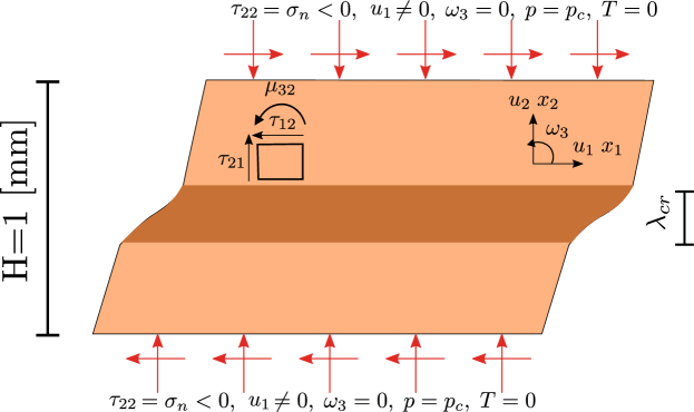
Figure 1: 1D consolidated Cosserat layer under shear.

2.8 Traveling instabilities

In this section, we advance beyond the linear stability analyses carried out in Rattez et al. (2018a), as we are mainly concerned with the behavior of the imaginary part of the complex eigenvalues defining the Lyapunov coefficient $s$. In the context of Lyapunov stability analysis the eigenvalues with positive real part show that the system is unstable. Moreover, if the eigenvalue in question is complex then the instability is characterized as a flutter instability (see Brauer and Nohel (1969)). In partial differential equations though, the appearance of imaginary parts in $s$ is associated to the nucleation of traveling waves as cited in Rice et al. (2014a); Platt et al. (2014a) and presented in Stathas and Stefanou (2022b). More specifically, by assuming a perturbation $\tilde{\phi}=[\tilde{u}_{i},\tilde{\omega}_{i},\tilde{T},\tilde{p}]$ of complex Lyapunov coefficient $s=s_{r}+s_{i}i$ and complex wavenumber $k=k_{r}+k_{i}i$ of the form:

$$\tilde{\phi}=\phi_{0}\exp(s_{r}\bar{t}+k_{i}x)\exp[i(s_{i}t+k_{r}\bar{x})],$$ (28)

where, $\phi_{0}=[u_{0},\omega_{0},T_{0},p_{0}]$, we observe that traveling perturbations appear in the medium, as the second factor or equation (28) becomes a sinusoidal.

The existence of the traveling perturbations together with the special kind of drained, isothermal, Dirichlet (essential) boundary conditions of the PDE system leads to reflection of the traveling perturbation near the fault gouge boundaries and may lead to the appearance of a limit cycle. We note here that the applied boundary conditions are extremely important for the behavior of the instability. Contrary to the previous case of Dirichlet conditions, In the case of adiabatic undrained (Neumann) boundary conditions, the spatial profiles of pressure and temperature do not allow for a reflection of the traveling instability at the boundaries and therefore, the perturbation stations in one of the boundaries of the model. The existence of a limit cycle and the traveling instability is a characteristic similar to the Portevin Le Chatelier effect found in metals (see Hähner et al., 2002; Mazière et al., 2010; Wang et al., 1997, among others). In the case of metals, the identified limit cycle, is attributed to the diffusion mechanisms present in the medium and the inherent coupling between balance and diffusion equations (see Benallal et al. (2006, 2008); Hähner et al. (2002); Mazière et al. (2010)).

We note that from the linear stability analysis of the previous system around the solution of homogeneous deformation (see Sulem et al. (2011)), the dominant perturbation does not have a complex Lyapunov coefficient. This, however, is not necessarily true around a localized solution away form the initial homogeneous deformation. In the last case the influence of the apparent softening due to thermal pressurization needs to be taken into account. Assuming a correspondence exists between the apparent softening and a mechanical softening parameter, we expect flutter instabilities to be present once the system starts exhibiting a softening behavior.

In Figure 2, we present the effect of the softening parameter $h$ on the localization length $\lambda_{r}$ of the maxima of the real and imaginary parts $(s_{r},s_{i})$ of the Lyapunov coefficient $s$. We note that the value of the real part of Lyapunov coefficient $s_{r}$ is negative for perturbations of zero wavelength, therefore no localization on a mathematical plane can occur, independently of the softening parameter $h$. This is to be expected in the case of a Cosserat continuum due to the introduction of an internal length, which regularizes the problem. Initially for small values of softening the wavelengths corresponding to the maxima of $s_{r},s_{i}$ do not match. The wavelength corresponding to the growing perturbation exhibits an unbounded positive real part and zero imaginary part for the Lyapunov coefficient. This means that at the initial stages of coseismic slip, the strain localization is not traveling in the medium. However, as yielding continues and thermal pressurization leads to more pronounced softening, the imaginary part catches up with the real part, meaning that both the maxima of the real and imaginary parts of the Lyapunov coefficient $s$ occur for the same perturbation wavelength. This leads to a traveling strain localization inside the layer (see Figure 2 and section 3).

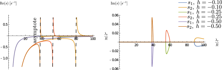
Figure 2: On the left: Real part of the two roots of the characteristic polynomial for different values of the hardening parameter h. There is always a critical wavelength value $\lambda_{cr}$ greater than zero, for which the Lyapunov exponent tends to infinity. On the right: Imaginary parts of the roots for the same softening values. As softening intensifies, positive real values of $s$ with non zero imaginary part appear on a $\lambda_{r}\neq 0$, leading to a traveling perturbation of a non zero critical wavelength.

For the value of the softening parameter $h_{s}=-0.50$ that produces the traveling perturbation of finite width, we further examine the effect of a non negative imaginary part in the wavenumber $k=k_{r}+k_{i}i$. The imaginary part of $k$ is responsible for the change of the perturbation amplitude with space. In a bounded problem such as the one discussed here, its effect is not important as the amplitude will remain bounded with distance. It is of interest, however, to examine whether traveling modes of strain localization are possible in the more general context. For a given value of the softening parameter $h_{s}$ and treating $k_{i}$ as a parameter, the plots of the real and imaginary part of the roots of the characteristic polynomial $s_{1,2}$ are shown in Figure 3. In the left part of Figure 3, we notice that localization on a mathematical plane is avoided for any $k_{i}$, since for $\lambda_{r}=0$ the real part of the Lyapunov coefficient $s$ tends to $-\infty$. This is in contrast with viscous regularization, where it was recently shown that strain localization on a mathematical plane is always possible (see Stathas and Stefanou (2022b)). This behavior is owed to the internal length introduced in the Cosserat continuum that regularizes effectively strain localization.

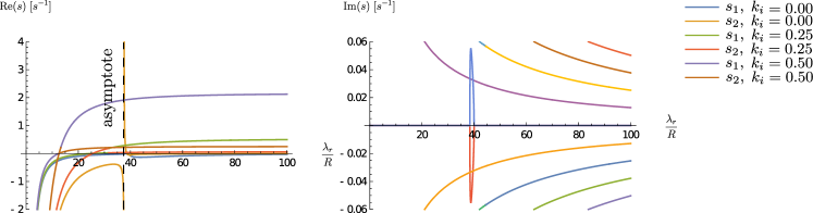
Figure 3: On the left: Real part of the two roots of the characteristic polynomial for different values of the attenuation coefficient $k_{i}$. The two roots start negative and eventually they pass to positive values for the real part of $s$. The wavelength each root changes its sign as well as the maximum value reached are characteristics of the value of $k_{i}$. On the right: Imaginary parts of the roots for the same softening values and values of the attenuation coefficient $k_{i}$. For $k_{i}\neq 0$, the magnitude of the imaginary part of the roots Im[$s_{1},s_{2}$] starts from $\infty$ when $\lambda_{r}=0$ and slowly attenuates. This is in high contrast to the behavior exhibited when $k_{i}=0$. The perturbation increasing the fastest is the one lying on $k_{i}=0$.

On the right part of Figure 3 we notice that the behavior of the imaginary part of the roots $s_{1},s_{2}$ is symmetric around $k_{i}=0$, as expected. Therefore, we focus our attention to values of $k_{i}>0$. The roots present a positive real part for a range of values of $\lambda_{r}$ (see Figure 3). For $k_{i}\neq 0$ the positive real part of the Lyapunov coefficient, $s_{r}=\text{Re}[s]$, is bounded and obtains its maximum value as $\lambda_{r}$ tends to $\infty$. For $k_{i}\neq 0$, the maximum value of the imaginary part of $s_{1,2}$ is obtained for $\lambda_{r}\rightarrow 0$ and then it slowly attenuates as $\lambda_{r}\rightarrow\infty$. Thus when $k_{i}\neq 0$ the uniform strain profile dominates. Finally, when $k_{i}=0$, we note again that Re$[s]\to+\infty$ and Im$[s]\neq 0$ at a finite value of $\lambda_{r}$. We conclude, from the above, that traveling perturbations of unbounded increasing amplitude and finite width are possible in the case $(s_{r}>0,s_{i}\neq 0,k_{i}=0)$.

3 Numerical Analyses

A 1D model of a Cosserat layer was used, where shear displacement was applied to the boundaries of the layer, while rotations were blocked at both ends. Figure 1 describes the model in more detail. The layer was discretized using 80 finite elements, with quadratic shape functions for the displacement field $u_{i}$ and linear shape functions for the rotations $\omega_{i}$. Reduced integration scheme was used for the displacement field compared to full for the rotation field (see Godio et al., 2016). These element parameters were taken as a result of a mesh convergence investigation of different shape functions and number of Gauss points that was performed in a previous work in order to find the optimal mesh description (see Stathas and Stefanou, 2019). The mesh characteristics are summarized in Table 1. The Cosserat material properties used to describe a mature fault in the seismogenic zone are summarized in Table 2, where a relatively high value for the friction coefficient $\mu$ has been used with respect to the values provided in Rice (2006b); Rempel and Rice (2006); Rice et al. (2014b) and path averaged values for $\lambda^{*}$, $\beta^{*}$ were considered, as proposed in Rice (2006a); Rice et al. (2014b).

	$u_{i}$	$\omega_{i}$
Element type	Quadratic	Linear
Integration scheme	Reduced	Full
Number of elements	80

Table 1: Mesh properties of the problem.

To illustrate the role of seismic slip velocity in the post peak behavior of the fault, we apply two different shear velocity-stepping programs to the model at hand. First we implement a three step procedure described in section 3.1 which includes, consolidation of the layer to the stresses and pressure at a depth representative of the seismogenic zone ($7$ km) followed by slow shear of the layer and then by fast shear for a shear slip of 10 mm at each stage. The second program in section 3.2 involves initial consolidation and then shear with constant slip velocity, $\dot{\delta}$, ranging from as slow as $0.01$ m/s to $1.0$ m/s for a total of 100 mm of seismic slip $\delta$.

Parameters	Values	Properties	Parameters	Values	Properties
$K$	$20.\;10^{3}$	MPa	$\mu$	$0.5$	-
$G$	$10.\;10^{3}$	MPa	$\beta$	$0$	-
$G_{c}$	$5.\;10^{3}$	MPa	$\lambda^{*}$	$13.45\;10^{-5}$	$/^{o}$C
$L$	$10^{3}$	MPa mm2	$\beta^{*}$	$8.2\;10^{-5}$	MPa${}^{-}1$
$M$	$1.5$	MPa mm2	$\rho C$	$2.8$	MPa/oC
$M_{c}$	$1.5$	MPa mm2	$c_{hy}$	$12.0$	mm2/s2
$R$	$0.01$	mm	$c_{th}$	$1.0$	mm2/s2
$\sigma_{n}$	$200$	MPa	$\alpha_{s}$	$10^{-5}$	$/^{o}$C
$p_{0}$	$66.67$	MPa	$\chi$	$12.\;10^{-15}$	m2

Table 2: Material parameters of a mature fault at the seismogenic depth (see Rice, 2006a; Rattez et al., 2018c).

A second series of analyses were also run, where the seismic slip displacement is set to 1 m and the seismic slip velocity to $1$ m/s - typical values observed in nature during large coseismic slip. All these analyses go far beyond the previous limit of $5$ mm presented in Rattez et al. (2018c, b), and allow us to observe new and interesting phenomena. The higher seismic slip displacement, allows us a deeper understanding of the phenomenon of thermal pressurization since it is shown that a traveling instability is formed inside the gouge due to the existence of a limit cycle in later parts of the analysis (see Figure 16). This behavior is new compared to previous analyses on the same mechanism of thermal pressurization done with simpler models (see Lachenbruch (1980); Rice (2006a); Rice et al. (2014a)).

Finally, in section 3.4, we illustrate here the effect of the boundaries in the traveling velocity $v$ of the PSZ inside fault gouge, by considering two different fault gouge layers of height 1 mm and 2 mm respectively subjected to the same seismic slip displacement $\delta$=1 m with seismic slip velocity $\dot{\delta}$=0.5 m/s. We note, based on the scaled system of equations (14), that the two configurations described here, differ only in the diffusion terms. Namely, the thicker layer diffuses pressure and temperature slower, exhibiting more pronounced apparent softening due to thermal pressurization.

3.1 Shearing of a mature fault gouge under small slip ($\delta=10$ mm) and velocity stepping

To better understand the effects of the applied shearing rate $\dot{\delta}$ in thermal pressurization and the overall effects of the boundary, as mentioned above, we proceed with the application of a velocity stepping shearing procedure. After consolidation (see Table 3), the layer is sheared with varying slip velocity $\dot{\delta}$ in two steps. At each step a target displacement $\delta$ of 5 mm at each end is reached for a total of 10 mm at the end of the analysis. The shear velocity $\dot{\delta}$ during the first shear step is $0.01$ m/s. For the second (final) step we ran different analyses under different applied constant shear velocity. The range of shear velocity values spans from $0.01$ m/s to $1$ m/s.

STEP		Slip $\delta$ mm	Slip velocity $\dot{\delta}$ m/s
0	Consolidation	-	-
1	Shear	5	0.01
2	Shear	5	0.01	0.1	1.0

Table 3: Loading program for the analyses performed using the three step procedure.

We intent to investigate the effect of the shearing rate on the frictional response of the layer. We investigate the predictions of our model concerning the apparent softening in the layer’s frictional response subjected to isothermal ($\Delta T$=0) drained ($\Delta P$=0) boundary conditions. In Figure 4 we compare the different shear stress $\tau$ seismic slip displacement $\delta$ responses for the different velocities applied at the final step of the analyses and we show the profiles of strain localization rate $\dot{\gamma}^{p}$ over the layer’s height. We observe that the increase of slip velocity $\dot{\delta}$ has a weakening effect on the $\tau-\delta$ diagram as observed also by Rattez et al. (2018c, a). This happens due to the fact that a fast increase in the heat production term of equation 6 leads to an increase in the thermal pressurization term of equation 7, which in turn increases pressure and intensifies weakening due to the application of Terzaghi principle $\sigma^{eff}=\sigma_{n}+p$, ($p>0$ water pressure, $\sigma^{eff},\sigma_{n}>0$ in tension). The increase of slip velocity leads also to narrower localization zones, which are in agreement with the steeper post-peak response observed in $\tau,{\delta}$ diagrams.

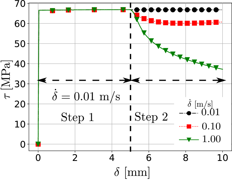
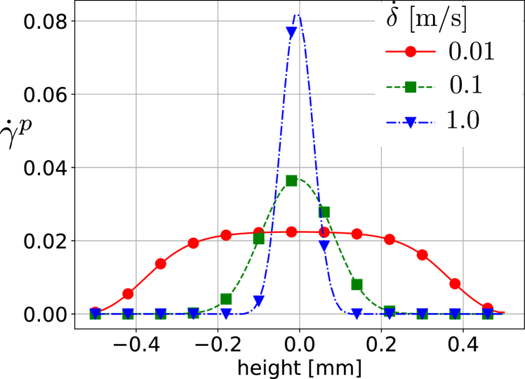
Figure 4: Left: $\tau-\delta$ response of the layer for different slip velocities $\dot{\delta}$ applied (velocity stepping). We observe that as the shearing rate increases, the softening behavior becomes more pronounced as a result of smaller localization widths due to the smaller characteristic diffusion time. Right: Profiles of strain localization rate inside the layer for different slip velocities $\dot{\delta}$ applied at the end of the analysis. Higher shearing velocities correspond to more localized plastic strain rate $\dot{\gamma}^{p}$ profiles.

Finally, we investigate the influence of the boundary conditions of pressure and temperature to the behavior of the problem. Their influence to the frictional response is of great importance as they control the effect of diffusion on leading temperature and pressure increase ($\Delta T,\Delta P$) away from the localized zone. On the left part of Figure 5 we present the curves of $\tau-\delta$, for slip velocity $\dot{\delta}$ at the final step of the analysis of 1 m/s, for adiabatic-undrained ($q_{T}=q_{p}=0$), isothermal-drained ($\Delta T=\Delta P=0$), isothermal-undrained ($\Delta T=q_{p}=0$) and adiabatic-drained conditions ($q_{T}=\Delta P=0$). We observe that undrained boundary conditions influence the response the most as they tend to follow on the solution of uniform adiabatic undrained shear described in Lachenbruch (1980) for small slip velocities $\dot{\delta}=0.01$ m/s. The difference at the peak strength between drained and undrained conditions has to do with the frequency our algorithm saves the output as well as the time increment used by the analysis (automatic time stepping). Furthermore, on the right of Figure 5 we present the plastic strain-rate profiles $\dot{\gamma}^{p}$ for different boundary conditions applied at the end of the analysis. We observe that for the given seismic slip of 10 mm, localization width is dependent on the seismic slip velocity applied and not on the boundary conditions.

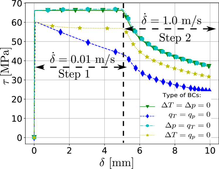
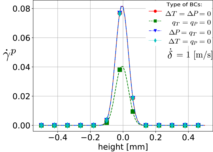
Figure 5: Left: $\tau-\delta$ response of the layer for different boundary conditions applied. An envelope is created between Isothermal drained ($\Delta T=\Delta P=0$) and Adiabatic-Undrained $(q_{T}=q_{p}=0)$ conditions. At the slow slip part of the analysis in the case of adiabatic undrained boundary conditions, thermal pressurization is present from the beginning. In this case, the initial stress at the start of the fast shear is lower and thus the stress drop is smaller. Right: Profiles of strain localization rate inside the layer for different boundary conditions. Since Cosserat material parameters and coseismic slip velocity $\dot{\delta}$ remain the same in all cases, the localization width does not change.

Based on the above results, we conclude that the true response of the fault gouge is very much dependent on the applied boundary conditions. Normally a kind of Robin boundary condition should be employed to better approximate the physical conditions. However, since this interaction between fluxes and essential boundary conditions is not yet sufficiently documented in the existing literature, the isothermal ($\Delta T=0$), drained ($\Delta p=0$) boundary conditions are closer to the real conditions due to the highly damaged regions encapsulating the fault gouge.

More specifically, the thermal diffusivity of the fault gouge and the surrounding material in the damaged zone (surrounding folliations) presents less variations than the corresponding hydraulic diffusivities. Thermal diffusivity of the fault gouge material can be one order of magnitude smaller than the diffusivity of the damaged zone (see for instance Passelègue et al., 2014; Tanaka et al., 2007; Yao et al., 2016). For the much more crucial hydraulic diffusivity parameter (see Aydin, 2000), the hydraulic diffucivity ratio between the mature fault gouge and the surrounding folliated rock can be shown to differ up to 4 orders of magnitude, with diffusivity of the folliated rock being greater than that of the gouge. Furthermore, according to in situ observations (see Ingebritsen and Manga, 2019) of increased water discharge to aquifiers, the ratio is expected to increase even more during coseismic slip. Therefore, we can estimate the ratios of thermal, $r_{th}$, and hydraulic, $r_{hy}$, diffusivities between the fault gouge material and the nearby damaged material:

$$r_{th}=\frac{c^{rc}_{th}}{c^{fg}_{th}}\sim 10,\;\;\;r_{hy}=\frac{c^{rc}_{hy}}{c^{fg}_{hy}}\sim 10^{4}$$ (29)

These parameters, further justify our choice of setting the boundary conditions in the rest of the paper to isothermal $\Delta T=0$ drained $\Delta P=0$.

3.2 Shearing of a mature fault under moderate slip ($\delta=100$ mm), and variable slip velocities

To better illustrate the dependence of the fault behavior to the velocity of seismic slip $\dot{\delta}$, we run a second part of analyses for the case of isothermal drained conditions ($\Delta T=\Delta P=0$) in which the intermediate part of slow shear velocity has been omitted and the fault model is immediately subjected to fast slip velocity rates after initial consolidation. Furthermore, the target seismic displacement $\delta$ has been increased to $100.0$ mm. We aim that way to examine in more detail the fault’s response under displacement scales commonly observed in nature at variable slip rates. Fast slip rates would correspond to the fault gouge being in the center of the fault rupture area. For the numerical steps of the simulations see Table 4.

STEP		Height H mm	Slip $\delta$ mm	Slip velocity $\dot{\delta}$ m/s
0	Consolidation	1	-	-
1	Shear		100.0	$\{0.01,0.05,0.1,0.25,0.50,0.75,0.90,1.0\}$
0	Consolidation	1	-	-
1	Shear		1000.0	1.0
0	Consolidation	1	-	-
1	Shear		1000.0	0.5
0	Consolidation	2	-	-
1	Shear		1000.0	0.5

Table 4: Loading program for the analyses performed using the two step procedure.

In Figure 6, we present the frictional response of the fault gouge, shear stress $\tau$, with the seismic slip $\delta$ on top of the layer. We plot the $\tau-\delta$ response for different values of seismic slip velocity. It can be clearly seen from the results that two behaviors are present depending on the shear velocity. If the slip velocity is low, then the layer accommodates the heat produced from the plastic work during yielding of the material and both heat and pressure diffuse efficiently away from the yielding zone, which has a comparatively large localization width $l_{loc}$ as shown in Figure 7. As slip velocity increases the post peak softening response is seen in larger parts of the analysis before eventually diffusion dominates and peak shear strength is restored. However, shear strength is only partially restored for the analyses of large shear velocities.

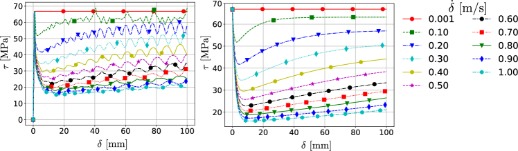
Figure 6: Left: $\tau-\delta$ response of the layer for different velocities. Isothermal, drained boundary conditions $\Delta T=\Delta P=0$ are applied. Frictional strength regain is observed due to the diffusion at the boundaries. The frictional response presents oscillations due to the traveling plastic strain rate instability. A smaller residual friction value is achieved. Right: Fitted $\tau-\delta$ response of the layer for different velocities, by filtering out the oscillations resulting form traveling instabilities. Isothermal, drained boundary conditions $\Delta T=\Delta P=0$ are applied. All analyses at the start reach the peak strength $\tau=66.67\;$MPa. As slip $\delta$ progresses an increase of the residual shear stress $\tau$ takes place.

In the left part of Figure 6 the frictional response ($\tau-\delta$) of the layer obtained from the numerical analyses of first row of Table 4 is presented. We notice the existence of oscillations in the frictional response for all velocities apart from the very small ($\dot{\delta}=0.01$ m/s). The oscillations start during the apparent softening branch of the analysis frictional response. They are affected by the boundaries of the model, namely in the case of undrained, adiabatic boundaries the shear band travels to one of the boundaries and then persists at this position, while for isothermal drained conditions an oscillatory response is present (see also sections 3.3,3.4 for more details about this important finding).

In the right part of Figure 6 we present the $\tau-\delta$ fit of the numerical results. We employ a function composed of an exponential decay and a logistic curve.

$$\tau(\delta,\dot{\delta})=a(\dot{\delta})\exp{\left[-b(\dot{\delta})\delta\right]}+\frac{c(\dot{\delta})}{d(\dot{\delta})+\exp\left[\right.-f(\dot{\delta})(\delta-\left.g(\dot{\delta}))\right]},$$ (30)

where $\alpha(\dot{\delta}),\;b(\dot{\delta}),\;c(\dot{\delta}),\;d(\dot{\delta})$ are the interpolation parameters, dependent on $\dot{\delta}$. The fit is used to simplify conceptually the results and highlight the main findings of the numerical analyses. It contains the initial frictional weakening and subsequent frictional regain due to the diffusion at the boundaries of the model. Furthermore, the effect of the oscillations is highlighted. The fit passes through the average of the oscillations of the numerical analyses, indicating that due to the oscillations, friction is not fully restored to its initial value. There exists a residual value of friction at the later stages of the slip.

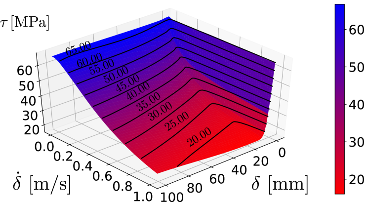
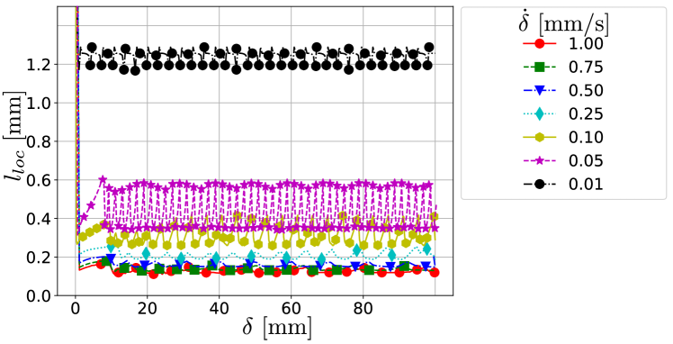
Figure 7: Left: 3D fitted surface of $\tau$ with slip distance $\delta$ and velocity $\dot{\delta}$. Right: $l_{loc}-\delta$ response of the localization width inside the layer for different boundary shear velocities applied at the boundaries.We notice that the localization width is oscillating for the small to intermediate range of shear velocities $\dot{\delta}=0.01-0.25$ m/s. This is due to the interaction between the diffusion lengths of pressure and temperature.

On the left part of Figure 7, we present the frictional surface that corresponds to the fit of the previous paragraph. Through the use of two dimensional interpolation of the results of Figure 6, we are able to estimate the frictional response of the fault gouge over a region of low to moderate seismic slips ($\delta=0\sim 0.1$ m) and seismic slip velocities ($\dot{\delta}=0.1\sim 1$ m/s).

On the right part of Figure 7, we present the evolution of the shear band width for the different seismic slip velocities. In order to estimate the localization width in each case a curve according to equation (31) described in Rice (2006a) was selected for fitting.

$$\dot{\gamma}^{p}= A+\frac{B}{\sqrt{1\pi}D}\exp\left[-\frac{1}{2}{\left(\frac{y-C}{D}\right)}^{2}\right]$$

$$l_{loc}= 2\sqrt{2\ln(2)}D$$ (31)

It is clear that large velocities lead to narrower localization widths $l_{loc}$. We observe that for large velocities localization width is not monotonously decreasing, but rather it exhibits some noise as shearing progresses. This goes beyond the results of Rattez et al. (2018a, c), where the localization width was shown to progressively decrease until it remains constant. This behavior has to do with the fact that the instability exhibited here by the material is a traveling wave instability.

This jerky behavior of frictional oscillations, which reminds the Portevin Le Chatelier effect can be responsible for higher frequency instabilities during seismic slip and enhance the frequency content of an earthquake event as discussed in Aki (1967); Brune (1970); Haskell (1964); Tsai and Hirth (2020). The observed behavior of frictional regain and frictional oscillations is primarily due to the applied isothermal drained boundary conditions that allow for a traveling PSZ inside the fault gouge. In the case of adiabatic undrained conditions the shear band can be shown to travel towards a boundary, where it is trapped for the duration of the analysis and the results obtained in this case are closer to those derived in the case of uniform shear (Lachenbruch (1980)).

3.3 Shearing of a mature fault for large slip $\delta=1\;\text{m}$ and coseismic slip velocity $\dot{\delta}=1\;\text{m/s}$.

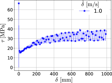
Figure 8: Left: Evolution of $\tau$ with slip distance $\delta$. We observe that after sufficient time has passed the oscillations have stabilized in amplitude and frequency partially recovering the layer’s initial shear strength. The steady state reached around which the oscillations take place is reached after a slip of 1.0 m. The value of friction at the steady state is a result of the interplay between the rate of work dissipated into heat and the diffusion properties of the fault gouge.

In order for the observed oscillations to fully develop in amplitude for the analyses with high slip rate $\dot{\delta}$ we apply a very large shear displacement. Figure 8, presents the $\tau,\delta$ response for a slip velocity $\dot{\delta}$ of 1 m/s and an applied slip $\delta=1$ m. As can be seen from the above analysis, the shear strength of the layer is eventually oscillating around a new residual strength value, which is smaller than the original peak strength.

The left part of Figure 9 shows the profiles of plastic strain rate $\dot{\gamma}^{p}$ and accumulated plastic strain $\gamma^{p}$ at the end of the coseismic slip. It is clear that the shear band travels across the fault gouge layer, since the accumulated plastic strain profile is larger in width than the localization width of the instability. This is one major difference compared to small slip rates, which our analyses under large displacements allowed to highlight (see Figure 6). Finally, the right part of Figure 9 presents the profiles of temperature $T$ and pressure $p$ at the end of the analysis. We observe that the temperature reached is much higher than the one required for the onset of melting for the minerals present in the seismogenic zone, see Rice (2006a). This has to do with the relatively high friction coefficient $\mu$ used in our analyses. A moderate value of $\mu$=0.25 would roughly halve the temperature observed. This does not preclude though other frictional weakening mechanisms, such as thermal decomposition of minerals (see Sulem and Famin (2009); Sulem and Stefanou (2016); Veveakis et al. (2014); Alevizos et al. (2014)), that might become dominant after thermal pressurization becomes impossible.

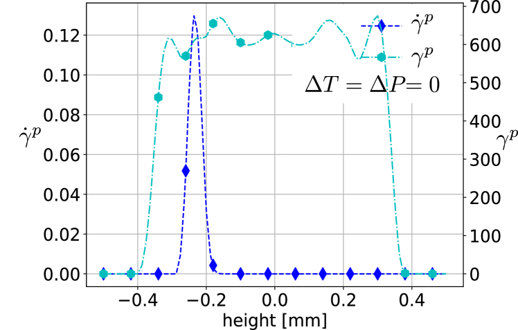
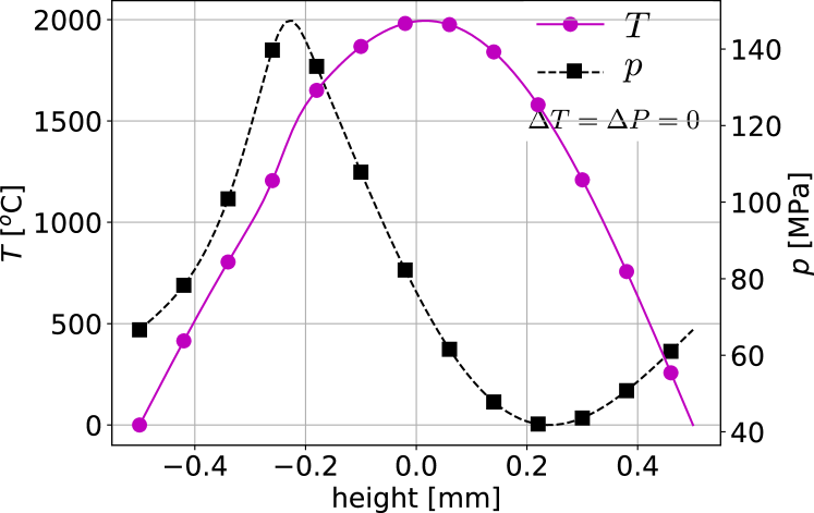
Figure 9: Left: Profiles of shear strain rate and accumulated plastic shear strain $\dot{\gamma}^{p},\gamma^{p}$ at the end of the analysis for applied slip $\delta=1$ m and slip rate $\dot{\delta}=$1 m/s. Since the two profiles differ, we conclude that the localization oscillates inside the layer. Localization does not travel the whole of the layer due to the boundary conditions applied. Right: Profiles of pressure and temperature $p,\;T$ at the end of the analysis for applied slip $\delta=1$ m and slip rate $\dot{\delta}=$1 m/s. Diffusion at the boundaries leads to extremely high values of temperature $\ T=$2000$\;{}^{o}$C.

A cycle of friction during the oscillation of the traveling shear band (PSZ) inside the fault gouge is separated in two stages: First the band travels inside the medium which corresponds to a weakening phase of the frictional response. The weakening phase takes place as the band travels across a hot region of the layer in which case according to equation (18) the pressure increases as $\Delta T$ is positive. Next, as the band travels inside the fault gouge expanding the yield zone, it approaches the boundaries. Close to the boundaries, temperature and pressure diffusion are more efficient. In particular, near the boundary, temperatures are lower as dictated by the parabolic profile of temperature $T$ (see Figure 9) due to diffusion. The high diffusion gradients result in the cooling of the region, where the shear band is present. This in turn leads to a decrease in the applied pressure, therefore, the layer regains part of its strength. During each cycle the yield region is slightly increasing and the oscillations grow in period, since the yield zone is progressively expanding, and in amplitude, since the cooling effect becomes more pronounced and the temperature gradients become steeper.

3.4 Effect of the layer’s height on the oscillations behavior

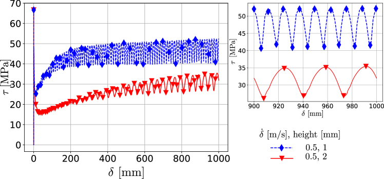
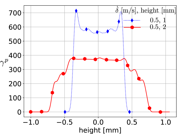
Figure 10: Left: Frictional strength evolution of two layers of width 1 mm (dashed , blue, diamond curve) and 2 mm (solid, red, triangle curve) under the same seismic slip velocity $\dot{\delta}=0.5$ m/s. Right: Profiles of accumulated plastic strain rate at the end of the two analyses. Yielding has not yet fully developed in the case of thickness of 2 mm.

In order to investigate how the boundaries affect the evolution of the traveling instability and of the frictional behavior inside the medium we compare the response between two layers of different height, 1 mm and 2 mm respectively, under a constant seismic slip velocity of 0.5 m/s (see Figure 10). We notice that the two layers exhibit a weakening response during the initial stages of thermal pressurization, however, the layer of thickness 2 mm reaches an overall lower minimum and a lower value for the residual shear strength. These values are essentially controlled by the diffusion processes. In the case of 1 mm, diffusion to the boundaries is more efficient and the layer regains more of its strength. Furthermore, diffusion is affected by the traveling instability inside the medium. In the case of the wider layer, from the period of the frictional strength oscillations (see inset of left part of Figure 10) we deduce that it takes almost twice the time for the traveling instability to cross through the layer. Therefore, temperature and pressure diffuse slower over the height of the layer. The period of the oscillations depends mainly on the height of the fault gouge layer.

The oscillations in the frictional response of the layer are dependent both in period and in amplitude on the height of the layer. Oscillations of higher amplitude occur in the case of the shorter layer height, where the plastic zone has more time to develop and the diffusion gradients close to the boundary are steeper. It is of paramount importance to take into account the slopes of $\tau$ w.r.t. $\delta$ both at the beginning and at the oscillation phase since they are vital for the instability nucleation in the various stick and slip models (see Dieterich (1992); Ruina (1983a); Rice (1973a)). For high velocities ($0.5\sim 1$ m/s) the slope at the beginning is the steepest and controls the energy balance (and the radiated energy), in contrast, for relatively small velocities ($0.1\sim 0.3$ m/s, see Figure 6) the trend might be different leading to radically different instability conditions. By calculating the radiated energy from an earthquake and having an accurate value for the seismic slip velocity $\dot{\delta}$, we can estimate the width of the fault gouge during the earthquake.

We note here that based on the discussion of section 2.6, applying a scaling that takes both into account the effect of coseismic velocity $\dot{\delta}$ and the characteristic height of the layer $\text{H}_{0}$, allows us to verify the above results. In essence we note that keeping the velocity constant, an increase in the layer’s height affects only the diffusion terms. In particular, the characteristic diffusion time $t_{0}$ doubles in the case of the thicker layer, indicating that the frictional regain due to the boundary effects will take more to develop. Note also that doubling the height of the layer leads to the doubling of the period in the thicker layer, indicating that the frictional oscillations depend on the diffusion properties of the fault gouge and its boundaries, and not on the characteristic length of the microstructure (Cosserat radius $R$).

3.5 Proposed mechanism for a traveling PSZ

We will proceed now to propose a mechanism that is responsible for the traveling of the strain localization (PSZ) inside the fault gouge. We consider initially two points inside the yielding region (PSZ): The first is lying in the middle of the localization while the second point lies in vicinity of the first one. Initially the temperature and the pore fluid pressure, increase faster in the middle of the layer. However, as the pore fluid pressure increases, friction inside the fault gouge drops due to the Terzaghi principle (apparent softening). This affects the thermal load due to dissipation inside the yielding region. In particular, the temperature increase in the middle is less than the corresponding temperature increase at the neighboring points of the yielding region, where dissipation is higher. Since temperature increases faster in the points near the middle than in the middle itself, the pore fluid pressure increase due to thermal pressurization is also greater in the neighborhood than in the middle.

The increase in the rate of pore fluid pressure indicates an increase in plastic strain rate in the neighboring points, because of the Terzaghi principle, which holds true also for the rates of fault friction and pore fluid pressure ($\dot{\tau}(t)=-\dot{p}(t)$). This increase of the plastic strain rate in the neighboring points corresponds to yielding accumulating away from the middle point. Thus the yielding region (i.e. the PSZ) starts traveling, following the accumulation of plastic strain rate. This leads to oscillations in the frictional response of the fault gouge. The crests of the oscillations correspond to the position of the PSZ lying closer to the boundaries of the fault gouge, while the troughs correspond to the PSZ in the middle of the fault gouge layer. The above mechanism embodies the finiteness of the yielding region.

4 Introduction of viscosity - rate and state phenomenology

Until now, a characteristic that is absent in the rate independent version of our model is the immediate positive frictional increase due to a sudden increase in the shearing velocity, due to viscous phenomena. These phenomena are considered in the frame of rate and state empirical models, through the ad hoc consideration of a velocity hardening term (see also Rice et al. (2001); Ruina (1983b, a); Dieterich (1992), $\alpha>0$ for rate strengthening). Adopting rate and state friction as a reference, as shown in Figure 11, this means that our model misses some necessary physics at the microscale like a creep mechanism at the asperity scale level and a notion of a state variable $\psi$ describing the contact behavior over time.

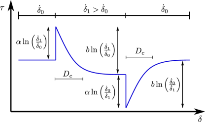
Figure 11: Rate and state phenomenology (image taken from Tzortzopoulos et al., 2021).

It should be emphasized that the role of the state variable $\psi$ is ambivalent, in the sense that rate and state formulations do not necessarily respect the basic thermodynamic principles, since they mostly result from fittings to experimental results. Furthermore, we still lack data in the pressure and temperature ranges usually expected at the seismogenic depth, therefore, the parameters used in these laws are crucial concerning the prediction of the frictional evolution during a seismic event (see Rice et al. (2001); Rice (2006b)). Recently, emphasis has been given into the thermodynamically consistent derivation of granular material constitutive laws (see Alaei et al. (2021)). These novel constitutive material formulations, lead to thermodynamically consistent models with the introduction of granular inertia effects, that successfully capture the rate and state behavior observed in the laboratory experiments under the laboratory observed temperature range.

We include rate dependence in the present THM coupled model by introducing viscosity, which will lead to a strain rate hardening (or softening) description. In particular, we assume a Perzyna elasto-viscoplastic material introducing strain rate hardening effects through the use of a viscosity parameter $\eta$. The THM coupled model discussed here with the introduction of viscosity, can replicate the immediate effects of rate and state model, without the introduction of extra material parameters or the notion of an internal state variable indicating the contact history. In this section we investigate the role of viscosity in the frictional behavior of the fault during coseismic slip. A velocity stepping procedure is followed in which the fault gouge is initially slipping with a small seismic slip velocity ($\dot{\delta}_{0}=0.01$ m/s) for a small seismic slip displacement ($\delta=10$ mm). Then an immediate increase in the seismic slip rate is enforced in the model ($\dot{\delta}=1.0$ m/s) to expose the rate dependence (see also Dieterich, 1992; Rice et al., 2001; Ruina, 1983b). We continue shearing until the seismic slip $\dot{\delta}$ reaches a value of 100 mm. Then, we perform a series of parametric analyses to determine the influence of the viscosity parameter $\eta$, mixture compressibility $\beta^{*}$, the size of the microstructure (Cosserat radius $R$) and the seismic slip velocity $\dot{\delta}$, in the frictional response of the fault.

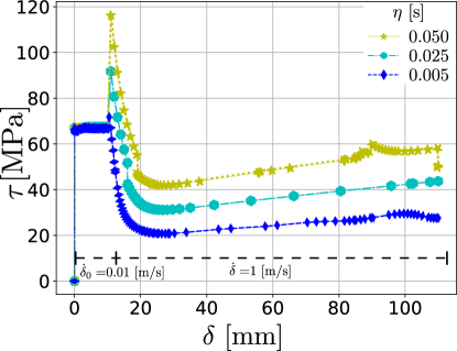
Figure 12: Evolution of the fault’s shear strength for a rapid change in shear rate $\dot{\delta}$ changes from 0.01 to 1.0 m/s, for different values of the viscosity parameter $\eta$. For large values of the viscosity parameter $\eta$ (star curve), stress drops and kinks corresponding to stick slip events are presented.

In Figure 12, we present the effect of the viscosity parameter in the frictional response of the fault for a sudden increase of the seismic slip rate from $\dot{\delta}_{0}=0.01$ m/s to $\dot{\delta}=1.0$ m/s. We observe that increasing the viscosity parameter $\eta$, the system becomes more sensitive to the sudden change of velocity reaching higher levels of peak frictional strength due to strain rate hardening. Three values are tested for the viscosity parameter $\eta=[0.005s,0.025s,0.05s]$, while the other material parameters are taken from Table 2. The lowest value corresponds to a meager increase in the fault’s frictional strength due to the change in the shearing rate and is well in agreement with the results for the rate independent model. The frictional response initially reaches a minimum leading to velocity weakening. Afterwards, friction starts increasing due to pressure diffusion and strain-rate hardening. For the other values of the viscosity parameter the frictional strength increase is important. This change in the viscosity parameter also affects the minimum value of the frictional strength and its corresponding seismic slip displacement $\delta$.

The viscosity parameter $\eta$ introduced in the THM model accounts for the positive shear rate dependence coefficient ($\alpha$) of the rate and state model. Typical values for the non-dimensional coefficient $\alpha$ for faults, lie in the range of $10^{-4}-10^{-3}$, thus the lower values of $\eta$ of our analyses leading to the estimation of $\alpha={\Delta\tau}/\left[\ln(\frac{\dot{\delta}}{\dot{\delta}_{0}})(\sigma_{n}-p_{f})f\right]=2\;10^{-4}$ correspond well to the stress rate increase predicted by the rate and state model (assuming scaling of $\eta$ with $\dot{E}=\frac{\dot{\delta}}{h}=1000\;\text{s}^{-1}$).

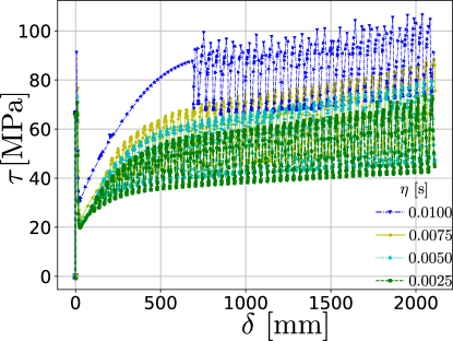
Figure 13: Evolution of the fault’s shear strength for viscous parameter $\eta$ for common values of the rate and state parameter $\alpha=10^{-4}-10^{-3}$ and large seismic slip displacements $\delta=2$ m. The strain rate hardening leads to a constant increase of the center of the oscillations, that tend to reach the overstrength value.

Next, we apply a higher seismic slip displacement $\delta$ equal to 2 m during the stage of fast shear for the low values of the viscosity parameter, in order to capture the response of our model for larger seismic slips. In Figure 13, we present the shear stress, seismic slip displacement $(\tau,\delta)$ evolution for shearing of a fault gouge with viscosity parameters $\eta$ in the range of [0.005 s - 0.010 s] for a seismic slip velocity, during the fast shear step, of $\dot{\delta}=1$ m/s. We note the small strain rate increase of the stress due to $\eta$ and the shear stress drop due to the apparent velocity weakening. The viscosity parameter enables the fault gouge to regain its overstrength in the latter analysis stages, since viscosity increases the localization width reducing frictional weakening due to thermal pressurization. We notice also that the oscillatory frictional response moves upward as seismic slip increases, while the oscillation maxima trace a curve of viscous evolution.

The oscillatory behavior of the frictional strength diagram could give rise to so called stick slip events in experiments. Thermal pressurization cannot completely halt strain-rate hardening, mainly due to the increased localization width the model exhibits, and the influence of the isothermal drained boundary conditions. We still can trace, however, a region of mild increases in the shear strength that can be used as an estimation of the characteristic weakening length, $D_{c}$, of the order of some centimeters (see also Di Toro et al. (2011) among others). We note here that the estimation of the $D_{c}$ in the context of thermal pressurization is different than in the case of rate and state, in the sense that in the case of rate and state friction, $D_{c}$ is independent of the shearing velocity (see Ruina, 1983a, among others). In our case the characteristic distance depends on the shear velocity $\dot{\delta}$ the viscous parameter $\eta$, the size of the microstructure $R$ and the pressure and temperature diffusion lengths of the problem.

Next, we explore the influence of the size of the microstructure (Cosserat radius) $R$, in the evolution of the fault’s frictional strength for a sudden change in the shearing rate from $\dot{\delta}=0.01$ m/s to 1 m/s (see Figure 14). We notice that an increase in the value of $R$ leads to higher shear overstrength due to the fast change in the shear rate. However, the post peak behavior changes little for values of $R$ varying from $0.1R_{ref}$ to $10R_{ref}$, where $R_{ref}$ is the Cosserat radius value in Table 2. For $R=100R_{ref}$ the increase in overstrength is substantial and the results show a faster regain of the strength and a higher minimum for the frictional strength after the initial apparent softening response.

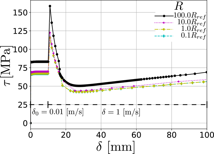
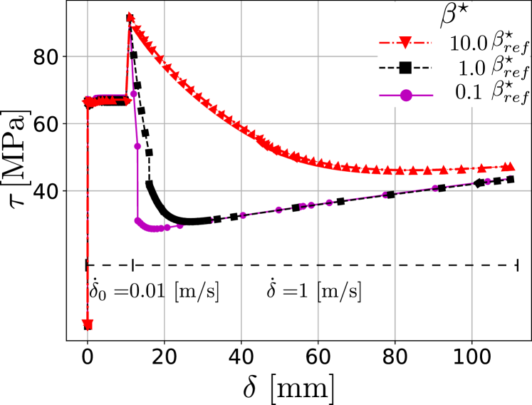
Figure 14: Left: Evolution of the fault’s shear strength for a rapid change in shear rate $\dot{\delta}$ from 0.01 to 1.0 m/s, for different values of the size of the microstructure (Cosserat radius, $R$ in mm). The response is largely unaffected by the increase of the internal length. Right: Evolution of the fault’s shear strength for a rapid change in shear rate $\dot{\delta}$ changes from 0.01 to 1.0 m/s, for different values of the mixture’s compressibility parameter $\beta^{\star}$ (MPa^-1). Increasing mixture’s compressibility leads to milder stress drops.

In Figure 14 on the right, we present the influence of the mixture compressibility parameter $\beta^{*}$ in the frictional response of the fault for a value of the viscosity parameter $\eta=0.025$ s and a fast seismic slip velocity of $\dot{\delta}=1$ m/s. The parameter $\beta^{*}$ affects two terms in the equation (7), namely the hydraulic diffusivity parameter $c_{hy}=\frac{\kappa}{\beta^{*}}$, where $\kappa$ is the permeability of the solid skeleton, and the term concerning the pressure decrease due to the porosity increase. Both these terms are affected the same by an increase (decrease) of $\beta^{*}$, however, the influence of the thermal pressurization term $\frac{\lambda^{*}}{\beta^{*}}$ decreases (increases) respectively. Taking the $\beta^{*}$ value for which we run the rate independent analyses as a reference value $\beta^{*}_{ref}$ (see Table 2), this corresponds to a smoother (in the case of $\beta^{*}=10\beta^{*}_{ref}$), or steeper (in the case of $\beta^{*}=0.1\beta^{*}_{ref}$) decrease of the peak frictional strength during the initial stages of the slip. The parameter $\beta^{*}$ also controls the minimum frictional strength of the fault and the seismic slip $\delta$ for which, the frictional strength increase due to diffusion will become prevalent. The results agree qualitatively well with the behavior observed in Badt et al. (2020) for higher compressibilities due to the formation of gouge material at the initial stages (see next section).

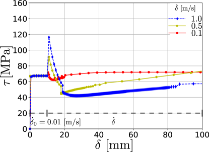
Figure 15: Frictional strength evolution of a Perzyna viscoplastic layer ($\eta=0.05$ s) under variable seismic slip velocities for a slip of $\delta=100$ mm.

Finally, in Figure 15, we explore the influence of the shearing velocity in the frictional strength behavior of the fault for constant compressibility and viscosity parameters $\beta^{s}=\beta^{s}_{ref}$ and $\eta=0.05$ s respectively. After the initial slow shear $\dot{\delta}=0.01$ m/s, we vary the fast shear velocity from $\dot{\delta}$=0.1 m/s to $1.0$ m/s. The model exhibits two distinct behaviors, according to the prescribed seismic slip velocity values $\dot{\delta}$. For the low velocities $\dot{\delta}=0.1\sim 0.2$ m/s we observe periodic kinks in shear strength during the phase of shear strength increase. For higher velocities we observe a snap-back behavior during the apparent softening phase of the model. Furthermore a secondary stick slip event is observed during the strength regaining phase of the simulation due to the diffusion.

The above results suggest that with the introduction of viscosity, our physics-based model can describe the rate and state phenomenology. For different values of the viscosity parameter $\eta$ as well as the permeability $\beta^{*}$, stick slip behavior can be observed. This behavior suggests that our model of thermal pressurization together with a Perzyna viscoplastic law applied on a conceptually simple Drucker Prager yield criterion can capture a lot of the characteristics proposed by heuristic, phenomenological models like the rate and state friction law and its variations. Moreover, it can give further insights about the physical processes taking place during coseismic slip.

5 Comparison with existing analytical solutions

We compare the nonlinear numerical solutions under adiabatic, undrained conditions ($q_{T}=q_{p}=0$) and isothermal, drained condtitions ($\Delta T=\Delta P=0$) to the reference analytical solutions obtained in bibliography for uniform shear of the layer (Lachenbruch (1980)), as well as the concentrated shear on the mathematical plane (Mase and Smith (1987); Rice (2006b)). The results are presented in Figure 16.

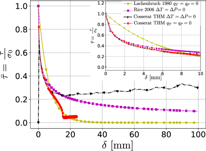
Figure 16: Comparison between the available numerical and analytical solutions for adiabatic undrained and isotropic drained conditions. The response of the Cosserat-THM model with isothermal drained boundary conditions (black-triangle line) lies close to the response of the slip on a plane solution provided in Rice (2006a) (purple-square line), for small values of coseismic slip ($\delta\leq 10$ mm). In the numerical model, localization is not constrained in a mathematical plane, leading to a steeper softening branch since more heat is produced in the yielding region enhancing thermal pressurization. Diffusion at the boundaries transfers heat and pressure away from the yielding region leading to partial strength regain causing a disagreement in the results. For the case of adiabatic undrained conditions, the Cosserat THM model (red-diamond line) eventually reaches the Lachenbruch solution (yellow-circle line).

For adiabatic undrained conditions, the Cosserat numerical solution with THM couplings tends to the Lachenbruch solution after sufficiently large slip $\delta$. For isothermal drained conditions the numerical solution initially lies close to the solution for slip on a mathematical plane given in Rice (2006b), however, the solution diverges as the seismic slip increases. This happens due to the diffusion at the isothermal drained boundary conditions, that restore part of the residual shear stress of the fault in later part of the analyses. The analytical solution for shear on a mathematical plane in Mase and Smith (1987); Rice (2006b), does not show this restrengthening behavior and the frictional oscillations. The reason is that the model in Rice (2006a) assumes that slip localizes on a stationary mathematical plane inside an infinite (unbounded) layer. The model in Mase and Smith (1987); Rice (2006b) neglects the ventilation phenomena that take place due to the interaction between the traveling PSZ (traveling thermal load) and the isothermal drained boundary conditions of the finite (bounded) fault gouge layer. In the companion paper (see Stathas and Stefanou (2022a)), we will extend the solution of slip on a mathematical plane, for the bounded fault gouge under isothermal drained boundary conditions and a traveling PSZ. The extended model then, can represent better the main underlying physics captured by the detailed numerical simulations presented in this paper.

It is worth pointing out, that the traveling instability discussed here has been observed also in Platt et al. (2014a); Rice et al. (2014a). However, the authors of that study applied periodic boundary conditions at the edges of the fault gouge instead of the isothermal drained conditions employed here. Furthermore, no connection was made in their model about the origin of these instabilities. Moreover, the authors did not comment on the effect of the traveling mode of strain localization (PSZ) on the layer’s frictional response. In this paper we have identified the source of the traveling oscillations as an instability resulting from a Hopf bifurcation, and commented on them extensively. It is worth emphasizing, that while our analyses and the model proposed in Rice (2006b); Platt et al. (2014a); Rice et al. (2014a) agree well with the dynamic weakening role of thermal pressurization at the initial stages of the phenomenon, they diverge in later stages of the analyses in particular due to the role of the boundary conditions affecting thermal and hydraulic diffusion in the fault gouge.

6 Comparison with existing experimental studies

The results of the numerical analyses presented in section 3 are also observed in experiments (see Badt et al. (2020); Di Toro et al. (2011); Rempe et al. (2020)). A great challenge seen in experimental studies about the role of thermal pressurization is the isolation of all other slip weakening mechanisms, in particular those of flash heating, silicate formation and thermal decomposition of minerals. Even bigger challenge is the replication of the exact ambient temperature and pressure conditions of the seismogenic zone. Moreover, the boundary conditions of the fault gouge, under which coseismic slip occurs are difficult to reproduce experimentally. Therefore, comparisons of analytical results to experimental findings are of a qualitative nature.

In Di Toro et al. (2011) the authors, have accumulated a large body of experiments performed at rates and displacement ranges comparable to those during seismic slip. The experiments were performed in a range of normal stresses of the order of 0.6 to 20 MPa. The authors advocate that for seismic slip velocities of the order of $1$ m/s the frictional stress drop is around $0.2-0.4$ of the initial strength with higher drop as the normal stress increases. The strength drop is of the same magnitude in our analyses (see Figure 10). Furthermore, the obtained experimental frictional response presents oscillations, which could be attributed to the Portevin Le Chatelier phenomenon, due to a traveling strain localization during shearing of the specimen. The authors of this study also introduce the thermal weakening distance $D_{th}$ that scales with the applied effective pressure on the specimen. From extrapolation of the available data to the pressure ranges found in the seismogenic zone, they estimate the weakening distance $D_{th}$ to be of the order of centimeters. This observation is consistent with our analyses. We note here that the boundary conditions adiabatic, undrained vs isothermal, drained, the height of the specimen and the thermal and hydraulic diffusivities ($c_{th},c_{hy}$), affect the calculation of $D_{th}$. In particular, fully saturated (wet) specimens of larger height under isothermal drained conditions will drop to lower values of friction before the effect of the boundaries becomes noticeable (see also section 3.4). The ratio between thermal and hydraulic diffusivities (Lewis number $Le=\frac{c_{th}}{c_{hy}}$), controls the frictional weakening due to thermal pressurization. We note here that the value of $c_{hy}$ affects the characteristic time after which the effects of the boundaries will be felt in the frictional response. Therefore, the minimum value of the frictional response is controlled by the ratio of the diffussivities $c_{th},c_{hy}$ and the height of the layer.

In the experiments performed in Badt et al. (2020), care was taken in order for the effect of thermal pressurization to be isolated from other weakening mechanisms. The authors of this study performed velocity stepping experiments in a rotary shear apparatus, with velocities of order $2.5\sim 5$ mm/s (well below the seismic range), under normal stresses of $20\sim 25$ MPa and confining pressure of $20\sim 49$ MPa for final values of slip $\delta=2.6$ m. The specimen’s height was $30$ mm. Their results suggest that frictional strength drops during the initial stages of thermal pressurization, while, depending on the evolution of the microstructure inside the fault (formation of fault gouge particles), partial regaining of the frictional strength is possible. The authors specify that steeper stress drop and restrengthening are observed in younger specimens that have not yet been subjected to large shear displacements ($\delta<1$ m) before the experiment. For specimens subjected to prior displacement the authors observe smoother stress drop and less tendency to regain frictional strength. They attribute this behavior to the formation of fault gouge inside the specimen that significantly affects the fault’s compressibility coefficient $\beta^{*}$ and therefore, the hydraulic diffusivity $c_{th}$.

Comparing with our numerical results and extrapolating to the in situ pressure range (after rescaling), we observe that our model agrees very well qualitatively with the experimental findings for the younger specimens (see Figure 17). Since our model does not possess a memory mechanism to account for the damage of the microstructure and, therefore, for the change in permeability, it suffices to say that the older specimens could be modeled with higher values for the hydraulic diffusivity $c_{hy}$. An expansion to our model could be made by taking into account a microstructure evolution model as the one considered in Collins-Craft et al. (2020). We note here, that based on the scaled system (14), the experimental results obtained during shearing of a specimen with height $\text{H}=30$ mm under a slip rate $\dot{\delta}=5$ mm/s, are comparable to our numerical experiments with fault gouge height $\text{H}=1$ mm and coseismic slip velocities in the range of $\dot{\delta}=100\sim 300$ mm/s (see section 2.6 for the appropriate scaling used).

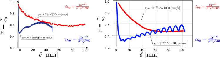
Figure 17: Qualitative comparison between experimental (left part of Figure) and numerical results (right part of Figure) examining the role of thermal pressurization. The experimental results were taken from Badt et al. (2020). The curves correspond to low (blue color) and high (red color) normalized hydraulic diffusivity values. In both cases shear velocity $\dot{\delta}$ and permeability $\chi$ influence heavily the results. Both the experiment and the numerical analysis predict frictional strength regain after the stress drop due to shear. The oscillatory frictional strength behavior of the numerical analyses is also present in the experiments of Badt et al. (2020) for low diffusivity values (blue curves). The experimental and numerical analyses are in qualitative agreement for normalized diffussivity values in the same parameter range.

7 Conclusions

In this paper we study the shearing of a fault gouge under large coseismic slip by considering a variety of seismic slip velocities $\dot{\delta}$ and seismic slip displacements $\delta$. First, we perform a linear stability analysis, indicating the possibility of traveling instabilities present in the medium. This result is further validated by the numerical results presented in section 3.3. The effect of the seismic slip velocity $\dot{\delta}$ on the apparent softening of the layer is presented, as well as the influence of the different boundary conditions considering the energy and mass balance equation (6), (7) equations respectively. It is shown that at the initial stages of the shearing (seismic slip $\delta$=$10$ mm), after shear strain localization, frictional weakening occurs for the different cases of boundary conditions (see Figure 5). The response, however, changes as the slip $\delta$ increases as shown in Figure 16. Next, we investigate the influence of the seismic slip velocity $\dot{\delta}$ on the frictional behavior under isothermal drained conditions $(\Delta T=\Delta P=0)$ for a seismic slip of $100$ mm (Figure 6). It is shown that after the initial slip rate-dependent apparent softening, the layer tends to regain part of its strength $\tau$, as slip $\delta$ accumulates due to the existence of a limit cycle.

In the presence of isothermal drained boundary conditions we observe that the fault gouge regains part of its frictional strength. Frictional regain depends on the seismic slip rate $\dot{\delta}$, the thermal and hydraulic diffusivity properties $(c_{th},c_{hy})$ and the height H of the gouge layer. Furthermore, we study the effects of the seismic slip rate on the evolution of the localization width $l_{loc}$. We notice the decrease of the localization width due to the increase in seismic slip velocity $\dot{\delta}$. This decrease indicates that the localization width is no longer dependent only on the Cosserat radius $R$, rather it is also dependent on the apparent softening due to thermal pressurization. There is an oscillatory behavior present in localization width particularly for low velocities. As the seismic slip rate increases, this oscillatory interaction reduces substantially. This further highlights the interplay between the different characteristic lengths in our model, in particular, between the Cosserat radius and the diffusion lengths.

Next, we study the evolution of the frictional resistance $\tau$ with seismic slip $\delta$ applying even larger seismic slip. In particular, we impose a realistic seismic slip displacement of $1$ m and seismic slip velocity of $1$ m/s. The oscillatory frictional behavior first described in Figure 6 for smaller slip is also present in Figure 8 for large coseismic slip. These frictional oscillations are the result of the PSZ traveling inside the fault gouge. We notice that in Figure 8, the frictional oscillations stabilize in frequency and amplitude. This implies a partial recovery of the frictional strength of the fault gouge, without it being explicitly implied by the mechanical behavior of the model as in the case of rate and state friction laws (see Dieterich, 1992; Rice et al., 2001; Ruina, 1983b). Because of the traveling PSZ, only partial frictional regain is possible during coseismic slip. We explore further this behavior in Part II, see Stathas and Stefanou (2022a).

During the isothermal drained analyses and the initial stages of the adiabatic undrained analyses, we observe oscillations in the fault’s frictional strength. This is a result of the traveling PSZ inside the fault gouge. The width and period of the oscillations depend on the height of the fault gouge. Frictional oscillations are the result of the high pressure and temperature diffusion gradients near the boundaries of the fault gouge. A similar result was achieved under periodic boundary conditions in Rice et al. (2014a), however, the authors did not comment on the nature of the traveling instability (traveling PSZ). A very important consequence of the traveling shear strain rate instability (PSZ) is the fact that field observations regarding the fault gouge and its width may not be accurate. This is because it is impossible to know the strain rate history inside the fault gouge (see Figure 9). As a consequence the principal slip zone inside the fault gouge may be smaller than the one identified by current experimental methods. Traveling instabilities may also offer an explanation to the formation of parallel slip zones as the ones examined in Nicchio et al. (2018).

We conclude our analyses, assuming a rate dependent material through the implementation of an elasto-viscoplastic Perzyna material with THM couplings. We notice that our model exhibits a strain rate hardening behavior after the sudden change of the shear rate. We further note that the value of the viscosity parameter $\eta$ controls important aspects of the simulation, such as the overstrength achieved due to the shearing rate, the existence and the magnitude of traveling instabilities (oscillations) in the solution, as well as the steady state the material reaches after sufficient shearing for varying shear rates. Overall, our Cosserat THM model with viscoplasticity is exhibiting a lot of the characteristics of a rate and state phenomenological model, without using an internal frictional state $\psi$ variable and its evolution law. The procedure of thermal pressurization has still a lot of potential explaining the frictional strength drop during an earthquake, together with the fault nucleation.

Finally, it can be shown that the results of the above numerical analyses agree qualitatively well with the recent experimental results obtained in Badt et al. (2020), where the thermal pressurization mechanism was studied in isolation to different frictional weakening mechanisms. Considering the evolution of the fault’s frictional strength with accumulated seismic slip, we observe that a single value for the characterization of the critical slip distance $D_{c}$ is not possible. Namely, according to Figure 8, the fault strength drops almost immediately after a slip of few centimeters to a minimum value close to 1/3 of the initial strength. This result agrees with extrapolations from experimental data to higher confining stresses (see Di Toro et al. (2011)). However, the final value around which the residual strength oscillates, is reached for a slip distance of $0.4$ m (see Figure 8). The latter result agrees with the estimation of Rempel and Rice (2006); Rice (2006b).

Our results are in contrast to the classical models of THM proposed in Lachenbruch (1980); Rice (2006a) that assume only monotonic reduction of the shear frictional strength during the seismic event. In order to understand the extreme difference between the predictions of the model described in Lachenbruch (1980); Rice (2006b) and our numerical results, we revisit in Part II (see Stathas and Stefanou, 2022a), the main assumptions of the theory of Rice (2006b) considering a traveling mode of strain localization and by modifying the boundary conditions.We will examine how each one of these parameters affect the theoretical predictions and will further justify our numerical results with Cosserat theory and THM couplings.

Appendix A Constitutive relations

The devolopement of the thermo-elasto-plastic constitutive ralations that follow is based on Sulem et al. (2011) and Rattez et al. (2018a). Since we follow a small strain approach, the strain rate and the curvature rate tensor can be decomposed into their elastic, plastic and thermal parts. Large displacements are then taken into account through an updated Lagrangian approach. In what follows we make the assumption that the curvature tensor stays unaffected by a change of temperature. Therefore strain rate and curvature rate tensors are decomposed as in Lemaitre et al. (2020):

$$\dot{\gamma}_{ij}= \dot{\gamma}^{e}_{ij}+\dot{\gamma}^{p}_{ij}+\dot{\gamma}^{th}_{ij},$$

$$\dot{\kappa}_{ij}= \dot{\kappa}^{e}_{ij}+\dot{\kappa}^{p}_{ij}$$ (32)

Thermal strain rates can be expressed as $\dot{\gamma}^{th}_{ij}=\alpha\dot{T}\delta_{ij}$, where $\alpha$ is the thermal expansion coefficient. For the calculation of the plastic strain rate, we first define a yield function $F=F(\tau_{ij},\sigma_{ij},\gamma^{p},\epsilon^{p}_{v})$, which we assume to be dependent only on the first and second stress tensor invariants as well as the deviatoric and spherical parts of the accumulated plastic strain tensor $F=F(\tau,\sigma,\gamma^{p},\epsilon^{p}_{v})$. A more complete approach in a thermodynamical framework that takes into account grain breakage and the consequent evolution of the internal lengths can be found in Collins-Craft et al. (2020). Following standard arguments of elasto-plasticity and by use of the consistency condition $\dot{F}$ we obtain:

$$\tau_{ij}=C^{e}_{ijkl}\left(\dot{\gamma}_{ij}-\dot{\gamma}^{p}_{ij}-\dot{\gamma}^{th}_{ij}\right),$$ (33)

$$\mu_{ij}=M^{e}_{ijkl}\left(\dot{\kappa}_{ij}-\dot{\kappa}^{p}_{ij}\right),$$ (34)

$$\dot{\gamma}^{p}_{ij}=\dot{\gamma}^{p}\frac{\partial Q}{\partial\tau_{ij}},$$ (35)

$$\dot{\kappa}^{p}_{ij}=\dot{\gamma}^{p}\frac{\partial Q}{\partial\mu_{ij}},$$ (36)

$$\dot{F}=\frac{\partial F}{\partial\tau_{ij}}\dot{\tau}_{ij}+\frac{\partial F}{\partial\mu_{ij}}\dot{\mu}_{ij}+\frac{\partial F}{\partial\gamma^{p}}\dot{\gamma}^{p}+\frac{\partial F}{\partial\epsilon^{p}_{v}}\dot{\epsilon}^{p}_{v}=0,$$ (37)

$$\dot{F}=\frac{\partial F}{\partial\tau}\dot{\tau}+\frac{\partial F}{\partial\sigma}\dot{\sigma}+\frac{\partial F}{\partial\gamma^{p}}\dot{\gamma}^{p}+\frac{\partial F}{\partial\epsilon^{p}_{v}}\dot{\epsilon}^{p}_{v}=0.$$ (38)

Where by $Q,\dot{\gamma}^{p}$ we denote the plastic potential and the plastic multiplier respectively. We note that in the present context a common criterion for both Cosserat stresses and moments has been assigned to the material. We continue by defining the hardening modulus $H_{s}$ as:

$$H_{s}= -\frac{\partial F}{\partial\gamma^{p}}.$$ (39)

Assuming a linear dependence of the yield and plastic potential functions to $\tau,\sigma$ as is the case in a Drucker-Prager material, which we will later use in the numerical analyses, the following relations hold for the plastic multiplier and the rate of volumetric plastic strain:

$$\dot{\gamma}^{p}=\dot{\gamma}^{p}\;\text{ and }\;\dot{\epsilon}^{p}_{v}=\beta\dot{\gamma}^{p}$$ (40)

where $\beta$ is the dilatancy angle. Multiplying (33) by $\frac{\partial F}{\partial\tau_{ij}}$ and (34) by $\frac{\partial F}{\partial\mu_{ij}}$ then adding together and taking advantage of the fact that $\frac{\partial F}{\partial\tau_{ij}}\dot{\tau}_{ij}+\frac{\partial F}{\partial\mu_{ij}}\dot{\mu}_{ij}=\frac{\partial F}{\partial\tau}\dot{\tau}+\frac{\partial F}{\partial\sigma}\dot{\sigma}$, the consistency condition yields:

$$\dot{\gamma}^{p}=\frac{<1>}{H_{p}}\left(\frac{\partial F}{\partial\tau_{ij}}C^{e}_{ijkl}(\dot{\gamma}_{kl}-\alpha\dot{T}\delta_{kl})\right)+\frac{\partial F}{\partial\mu_{ij}}M^{e}_{ijkl}\dot{\kappa}_{kl}.$$ (41)

Simplifying the notation we get:

$$\dot{\gamma}^{p}=\frac{<1>}{H_{p}}(b^{F}_{kl}(\dot{\gamma}_{kl}-\alpha\dot{T}\delta_{kl})+b^{F}_{kl}\dot{\kappa}_{kl}),$$ (42)

with

$$H_{p}=\frac{\partial F}{\partial\tau_{ij}}C^{e}_{ijkl}\frac{\partial Q}{\partial\tau_{kl}}+\frac{\partial F}{\partial\mu_{ij}}M^{e}_{ijkl}\frac{\partial Q}{\partial\mu_{kl}}+H_{s}$$ (43)

$$<1>= \begin{cases}1&\text{if $F=0$ and $\dot{\gamma}^{p}>0$}\\ 0&\text{otherwise}\end{cases}$$ (44)

and

$$b^{F}_{kl}=\frac{\partial F}{\partial\tau_{ij}C^{e}_{ijkl}},$$ (45)

$$b^{Q}_{ij}=C^{e}_{ijkl}\frac{\partial Q}{\partial\tau_{kl}},$$ (46)

$$b^{F}M_{kl}=\frac{\partial F}{\partial\mu_{ij}M^{e}_{ijkl}},$$ (47)

$$b^{Q}M_{ij}=M^{e}_{ijkl}\frac{\partial Q}{\partial\mu_{kl}}.$$ (48)

Using (35),(36) and (42) in (33) we obtain:

$$\dot{\tau}_{ij}=C^{ep}_{ijkl}\dot{\gamma}_{kl}+D^{ep}_{ijkl}\dot{\kappa}_{kl}+E^{ep}_{ijkl}\dot{T}\delta_{kl}$$ (50)

$$\dot{\mu}_{ij}=M^{ep}_{ijkl}\dot{\kappa}_{kl}+L^{ep}_{ijkl}\dot{\gamma}_{kl}+N^{ep}_{ijkl}\dot{T}\delta_{kl}$$ (51)

with

$$C^{ep}_{ijkl}=C^{e}_{ijkl}-\frac{<1>}{H_{p}}b^{Q}_{ij}b^{F}_{kl},$$

$$D^{ep}_{ijkl}=-\frac{<1>}{H_{p}}b^{Q}_{ij}b^{F}M_{kl},$$

$$E^{ep}_{ijkl}=-\left(C^{e}_{ijkl}-\frac{<1>}{H_{p}}b^{Q}_{ij}b^{F}_{kl}\right),$$

$$L^{ep}_{ijkl}=-\frac{<1>}{H_{p}}b^{Q}M_{ij}b^{F}_{kl},$$

$$M^{ep}_{ijkl}=\left(M^{e}_{ijkl}-\frac{<1>}{H_{p}}b^{Q}M_{ij}b^{F}M_{kl}\right),$$

$$N^{ep}_{ijkl}=\frac{<1>}{H_{p}}b^{Q}M_{ij}b^{F}_{kl}.$$ (52)

References

- Aki (1967) Aki, K., 1967. Scaling law of seismic spectrum. Journal of Geophysical Research 72, 1217–1231. doi:10.1029/jz072i004p01217.
- Alaei et al. (2021) Alaei, E., Marks, B., Einav, I., 2021. A hydrodynamic-plastic formulation for modelling sand using a minimal set of parameters. Journal of the Mechanics and Physics of Solids 151, 104388. URL: https://doi.org/10.1016/j.jmps.2021.104388, doi:10.1016/j.jmps.2021.104388.
- Alevizos et al. (2014) Alevizos, S., Poulet, T., Veveakis, E., 2014. Thermo-poro-mechanics of chemically active creeping faults. 1: Theory and steady state considerations. Journal of Geophysical Research: Solid Earth 119, 4558–4582. doi:10.1002/2013JB010070.
- Andrews (2005) Andrews, D.J., 2005. Rupture dynamics with energy loss outside the slip zone. Journal of Geophysical Research: Solid Earth 110, 1–14. doi:10.1029/2004JB003191.
- Aydin (2000) Aydin, A., 2000. Fractures, faults, and hydrocarbon entrapment, migration and flow. Marine and petroleum geology 17, 797–814.
- Badt et al. (2020) Badt, N.Z., Tullis, T.E., Hirth, G., Goldsby, D.L., 2020. Thermal Pressurization Weakening in Laboratory Experiments. Journal of Geophysical Research: Solid Earth 125, 1–21. doi:10.1029/2019JB018872.
- Benallal et al. (2006) Benallal, A., Berstad, T., Børvik, T., Clausen, A., Hopperstad, O., 2006. Dynamic strain aging and related instabilities: experimental, theoretical and numerical aspects. European Journal of Mechanics - A/Solids 25, 397–424. URL: https://www.sciencedirect.com/science/article/pii/S0997753805001440, doi:https://doi.org/10.1016/j.euromechsol.2005.10.007.
- Benallal et al. (2008) Benallal, A., Berstad, T., Børvik, T., Hopperstad, O., Koutiri, I., de Codes, R.N., 2008. An experimental and numerical investigation of the behaviour of aa5083 aluminium alloy in presence of the portevin–le chatelier effect. International Journal of Plasticity 24, 1916–1945. URL: https://www.sciencedirect.com/science/article/pii/S0749641908000570, doi:https://doi.org/10.1016/j.ijplas.2008.03.008. special Issue in Honor of Jean-Louis Chaboche.
- de Borst and Sluys (1991) de Borst, R., Sluys, L.J., 1991. Localisation in a Cosserat continuum under static and dynamic loading conditions. Computer Methods in Applied Mechanics and Engineering 90, 805–827. doi:10.1016/0045-7825(91)90185-9.
- Brauer and Nohel (1969) Brauer, F., Nohel, J., 1969. The Qualitative Theory of Ordinary Differential Equations: An Introduction. Dover Publications, New York.
- Brune (1970) Brune, J.N., 1970. Tectonic stress and the spectra of seismic shear waves from earthquakes. J Geophys Res 75, 4997–5009. doi:10.1029/jb075i026p04997.
- Collins-Craft et al. (2020) Collins-Craft, N.A., Stefanou, I., Sulem, J., Einav, I., 2020. A cosserat breakage mechanics model for brittle granular media. Journal of the Mechanics and Physics of Solids , 103975.
- Coussy (2004) Coussy, O., 2004. Poromechanics. John Wiley & Sons. doi:https://doi.org/10.1002/9780470710388.
- Di Toro et al. (2011) Di Toro, G., Han, R., Hirose, T., De Paola, N., Nielsen, S., Mizoguchi, K., Ferri, F., Cocco, M., Shimamoto, T., 2011. Fault lubrication during earthquakes. Nature 471, 494–499. doi:10.1038/nature09838.
- Dieterich (1992) Dieterich, J.H., 1992. Earthquake nucleation on faults with rate-and state-dependent strength. Tectonophysics 211, 115–134. doi:https://doi.org/10.1016/0040-1951(92)90055-B.
- Donea et al. (2004) Donea, J., Huerta, A., Ponthot, J., 2004. Chapter 14: Arbitrary Lagrangian–Eulerian Methods. Encyclopedia of Computational , 1–25URL: http://scholar.google.com/scholar?hl=en{&}btnG=Search{&}q=intitle:Chapter+14+Arbitrary+Lagrangian?Eulerian+Methods{#}2.
- Eringen (1968) Eringen, A.C., 1968. Mechanics of micromorphic continua, in: Mechanics of generalized continua. Springer, pp. 18–35.
- Forest (2020) Forest, S., 2020. Continuum thermomechanics of nonlinear micromorphic, strain and stress gradient media. Philosophical Transactions of the Royal Society A 378, 20190169.
- Forest et al. (2001a) Forest, S., Boubidi, P., Sievert, R., 2001a. Strain localization patterns at a crack tip in generalized single crystal plasticity. Scripta Materialia 44, 953–958.
- Forest et al. (2001b) Forest, S., Pradel, F., Sab, K., 2001b. Asymptotic analysis of heterogeneous Cosserat media. International Journal of Solids and Structures 38, 4585–4608. doi:10.1016/S0020-7683(00)00295-X.
- Forest and Sievert (2003) Forest, S., Sievert, R., 2003. Elastoviscoplastic constitutive frameworks for generalized continua. Acta Mechanica 160, 71–111. doi:10.1007/s00707-002-0975-0.
- Germain (1973) Germain, P., 1973. The method of virtual power in continuum mechanics. part 2: Microstructure. SIAM Journal on Applied Mathematics 25, 556–575.
- Godio et al. (2016) Godio, M., Stefanou, I., Sab, K., Sulem, J., 2016. Multisurface plasticity for cosserat materials: plate element implementation and validation. International Journal for Numerical Methods in Engineering 108, 456–484. doi:https://doi.org/10.1002/nme.5219.
- Hähner et al. (2002) Hähner, P., Ziegenbein, A., Rizzi, E., Neuhäuser, H., 2002. Spatiotemporal analysis of Portevin-Le Châtelier deformation bands: Theory, simulation, and experiment. Physical Review B - Condensed Matter and Materials Physics 65, 1–20. doi:10.1103/PhysRevB.65.134109.
- Haskell (1964) Haskell, N.A., 1964. Energy Wave and Energy From By Density of Elastic Radiation Propagating Faults. Bulletin of the Seismological Society of America 54, 1811–1841.
- Ingebritsen and Manga (2019) Ingebritsen, S., Manga, M., 2019. Earthquake hydrogeology. Water Resources Research 55, 5212–5216.
- Kanamori and Brodsky (2004) Kanamori, H., Brodsky, E.E., 2004. The physics of earthquakes. Reports on Progress in Physics 67, 1429–1496. doi:10.1088/0034-4885/67/8/R03.
- Lachenbruch (1980) Lachenbruch, A.H., 1980. Frictional heating, fluid pressure, and the resistance to fault motion. Journal of Geophysical Research: Solid Earth 85, 6097–6112. doi:https://doi.org/10.1029/JB085iB11p06097.
- Lemaitre et al. (2020) Lemaitre, J., Chaboche, J.L., Benallal, A., Desmorat, R., 2020. Mécanique des matériaux solides-3e éd. Dunod.
- Mase and Smith (1987) Mase, C.W., Smith, L., 1987. Effects of frictional heating on the thermal, hydrologic, and mechanical response of a fault. Journal of Geophysical Research 92, 6249–6272. doi:10.1029/JB092iB07p06249.
- Mazière et al. (2010) Mazière, M., Besson, J., Forest, S., Tanguy, B., Chalons, H., Vogel, F., 2010. Numerical aspects in the finite element simulation of the Portevin-Le Chatelier effect. Computer Methods in Applied Mechanics and Engineering doi:10.1016/j.cma.2009.11.004.
- Muhlhaus and Vardoulakis (1988) Muhlhaus, H.B., Vardoulakis, I., 1988. The thickness of shear hands in granular materials. Géotechnique 38, 331–331. doi:10.1680/geot.1988.38.2.331b.
- Myers and Aydin (2004) Myers, R., Aydin, A., 2004. The evolution of faults formed by shearing across joint zones in sandstone. Journal of Structural Geology 26, 947–966.
- Needleman (1988) Needleman, A., 1988. Material rate dependence and mesh sensitivity in localization problems. Computer methods in applied mechanics and engineering 67, 69–85. doi:https://doi.org/10.1016/0045-7825(88)90069-2.
- Nicchio et al. (2018) Nicchio, M.A., Nogueira, F.C., Balsamo, F., Souza, J.A., Carvalho, B.R., Bezerra, F.H., 2018. Development of cataclastic foliation in deformation bands in feldspar-rich conglomerates of the rio do peixe basin, ne brazil. Journal of Structural Geology 107, 132–141. doi:https://doi.org/10.1016/j.jsg.2017.12.013.
- Passelègue et al. (2014) Passelègue, F.X., Goldsby, D.L., Fabbri, O., 2014. The influence of ambient fault temperature on flash-heating phenomena. Geophysical Research Letters 41, 828–835.
- Platt et al. (2014a) Platt, J.D., Rudnicki, J.W., Rice, J.R., 2014a. Stability and localization of rapid shear in fluid-saturated fault gouge: 2. localized zone width and strength evolution. Journal of Geophysical Research: Solid Earth 119, 4334–4359. doi:https://doi.org/10.1002/2013JB010711.
- Platt et al. (2014b) Platt, J.D., Rudnicki, J.W., Rice, J.R., 2014b. Stability and localization of rapid shear in fluid-saturated fault gouge: 2. Localized zone width and strength evolution. Journal of Geophysical Research: Solid Earth 119, 4334–4359. doi:10.1002/2013JB010711.
- Puzrin and Houlsby (2001) Puzrin, A., Houlsby, G., 2001. On the thermodynamics of porous continua. Report No OUEL 2235. doi:https://doi.org/10.1007/978-3-540-35724-7_3.
- Rattez et al. (2018a) Rattez, H., Stefanou, I., Sulem, J., 2018a. The importance of Thermo-Hydro-Mechanical couplings and microstructure to strain localization in 3D continua with application to seismic faults. Part I: Theory and linear stability analysis. Journal of the Mechanics and Physics of Solids 115, 54–76. URL: https://doi.org/10.1016/j.jmps.2018.03.004, doi:10.1016/j.jmps.2018.03.004.
- Rattez et al. (2018b) Rattez, H., Stefanou, I., Sulem, J., Veveakis, M., Poulet, T., 2018b. Numerical analysis of strain localization in rocks with thermo-hydro-mechanical couplings using cosserat continuum. Rock Mechanics and Rock Engineering 51, 3295–3311.
- Rattez et al. (2018c) Rattez, H., Stefanou, I., Sulem, J., Veveakis, M., Poulet, T., 2018c. The importance of Thermo-Hydro-Mechanical couplings and microstructure to strain localization in 3D continua with application to seismic faults. Part II: Numerical implementation and post-bifurcation analysis. Journal of the Mechanics and Physics of Solids doi:10.1016/j.jmps.2018.03.003.
- Rempe et al. (2020) Rempe, M., Di Toro, G., Mitchell, T.M., Smith, S.A., Hirose, T., Renner, J., 2020. Influence of Effective Stress and Pore Fluid Pressure on Fault Strength and Slip Localization in Carbonate Slip Zones. Journal of Geophysical Research: Solid Earth 125. doi:10.1029/2020JB019805.
- Rempel and Rice (2006) Rempel, A.W., Rice, J.R., 2006. Thermal pressurization and onset of melting in fault zones. Journal of Geophysical Research: Solid Earth 111. doi:10.1029/2006JB004314.
- Rice (1973a) Rice, J.R., 1973a. The growth of slip surfaces in the progressive failure of over-consolidated clay. Proceedings of the Royal Society of London. A. Mathematical and Physical Sciences 332, 527–548. doi:10.1098/rspa.1973.0040.
- Rice (1973b) Rice, J.R., 1973b. The growth of slip surfaces in the progressive failure of over-consolidated clay. Proceedings of the Royal Society of London. A. Mathematical and Physical Sciences 332, 527–548. doi:10.1098/rspa.1973.0040.
- Rice (2006a) Rice, J.R., 2006a. Heating and weakening of faults during earthquake slip. Journal of Geophysical Research: Solid Earth 111. doi:https://doi.org/10.1029/2005JB004006.
- Rice (2006b) Rice, J.R., 2006b. Heating and weakening of faults during earthquake slip. Journal of Geophysical Research: Solid Earth 111, 1–29. doi:10.1029/2005JB004006.
- Rice et al. (2001) Rice, J.R., Lapusta, N., Ranjith, K., 2001. Rate and state dependent friction and the stability of sliding between elastically deformable solids. Journal of the Mechanics and Physics of Solids 49, 1865–1898. doi:10.1016/S0022-5096(01)00042-4.
- Rice et al. (2014a) Rice, J.R., Rudnicki, J.W., Platt, J.D., 2014a. Stability and localization of rapid shear in fluid-saturated fault gouge: 1. linearized stability analysis. Journal of Geophysical Research: Solid Earth 119, 4311–4333. doi:https://doi.org/10.1002/2013JB010710.
- Rice et al. (2014b) Rice, J.R., Rudnicki, J.W., Platt, J.D., 2014b. Stability and localization of rapid shear in fluid-saturated fault gouge: 1. Linearized stability analysis. Journal of Geophysical Research: Solid Earth 119, 4311–4333. doi:10.1002/2013JB010710.
- Ruina (1983a) Ruina, A., 1983a. Slip instability and state variable friction laws. Journal of Geophysical Research: Solid Earth 88, 10359–10370. doi:https://doi.org/10.1029/JB088iB12p10359.
- Ruina (1983b) Ruina, A., 1983b. Slip instability and state variable friction laws. Journal of Geophysical Research 88, 10359–10370. doi:10.1029/JB088iB12p10359.
- Sibson (1977) Sibson, R., 1977. Fault rocks and fault mechanisms. Journal of the Geological Society 133, 191–213.
- Sibson (2003) Sibson, R.H., 2003. Thickness of the Seismic Slip Zone. Bulletin of the Seismological Society of America 93, 1169–1178. URL: https://doi.org/10.1785/0120020061, doi:10.1785/0120020061.
- Stathas and Stefanou (2019) Stathas, A., Stefanou, I., 2019. Elastoplastic response of a cosserat continuum layer for application in fault mechanics. 12th HSTAM International Congress on Mechanics Thessaloniki, Greece, 22 – 25 September 2019 .
- Stathas and Stefanou (2022a) Stathas, A., Stefanou, I., 2022a. Fault friction under thermal pressurization during large coseismic-slip part ii: Expansion to the model of frictional slip. - -, –.
- Stathas and Stefanou (2022b) Stathas, A., Stefanou, I., 2022b. The role of viscous regularization in dynamical problems, strain localization and mesh dependency. Computer Methods in Applied Mechanics and Engineering 388, 114185.
- Stefanou et al. (2016) Stefanou, I., Sulem, J., Rattez, H., 2016. Cosserat approach to localization in geomaterials doi:https://doi.org/10.1007/978-3-319-22977-5_10-1.
- Strogatz (2000) Strogatz, S.H., 2000. Nonlinear Dynamics and Chaos: With Applications to Physics, Biology, Chemistry and Engineering. Westview Press.
- Sulem and Famin (2009) Sulem, J., Famin, V., 2009. Thermal decomposition of carbonates in fault zones: Slip-weakening and temperature-limiting effects. Journal of Geophysical Research: Solid Earth 114, 1–14. doi:10.1029/2008jb006004.
- Sulem and Stefanou (2016) Sulem, J., Stefanou, I., 2016. Thermal and chemical effects in shear and compaction bands. Geomechanics for Energy and the Environment 6, 4–21. URL: http://dx.doi.org/10.1016/j.gete.2015.12.004, doi:10.1016/j.gete.2015.12.004.
- Sulem et al. (2011) Sulem, J., Stefanou, I., Veveakis, E., 2011. Stability analysis of undrained adiabatic shearing of a rock layer with cosserat microstructure. Granular Matter 13, 261–268. doi:https://doi.org/10.1007/s10035-010-0244-1.
- Tanaka et al. (2007) Tanaka, H., Chen, W., Kawabata, K., Urata, N., 2007. Thermal properties across the chelungpu fault zone and evaluations of positive thermal anomaly on the slip zones: Are these residuals of heat from faulting? Geophysical Research Letters 34.
- Tsai and Hirth (2020) Tsai, V.C., Hirth, G., 2020. Elastic Impact Consequences for High-Frequency Earthquake Ground Motion. Geophysical Research Letters 47, 1–8. doi:10.1029/2019GL086302.
- Tzortzopoulos et al. (2021) Tzortzopoulos, G., Braun, P., Stefanou, I., 2021. Absorbent porous paper reveals how earthquakes could be mitigated. Geophysical Research Letters 48, e2020GL090792.
- Vardoulakis (1986) Vardoulakis, I., 1986. Dynamic stability analysis of undrained simple shear on water-saturated granular soils. International journal for numerical and analytical methods in geomechanics 10, 177–190. doi:https://doi.org/10.1002/nag.1610100206.
- Vardoulakis (1996) Vardoulakis, I., 1996. Deformation of water-saturated sand: I. uniform undrained deformation and shear banding. Géotechnique 46, 441–456.
- Vardoulakis (2018) Vardoulakis, I., 2018. Cosserat Continuum Mechanics: With Applications to Granular Media. volume 87. Springer. doi:https://doi.org/10.1007/978-3-319-95156-0.
- Veveakis et al. (2014) Veveakis, E., Poulet, T., Alevizos, S., 2014. Thermo-poro-mechanics of chemically active creeping faults: 2. Transient considerations. Journal of Geophysical Research: Solid Earth 119, 4583–4605. doi:10.1002/2013JB010071.
- Viesca and Garagash (2015) Viesca, R.C., Garagash, D.I., 2015. Ubiquitous weakening of faults due to thermal pressurization. Nature Geoscience 8, 875–879. doi:https://doi.org/10.1038/ngeo2554.
- Wang et al. (1997) Wang, W., Sluys, L., De Borst, R., 1997. Viscoplasticity for instabilities due to strain softening and strain-rate softening. International Journal for Numerical Methods in Engineering 40, 3839–3864. doi:https://doi.org/10.1002/(SICI)1097-0207(19971030)40:20<3839::AID-NME245>3.0.CO;2-6.
- Yao et al. (2016) Yao, L., Ma, S., Platt, J.D., Niemeijer, A.R., Shimamoto, T., 2016. The crucial role of temperature in high-velocity weakening of faults: Experiments on gouge using host blocks with different thermal conductivities. Geology 44, 63–66.